133
Shoreline – Shoreface Dynamics on the Suffolk Coast Marine Research Report

Shoreline – Shoreface Dynamics on the
Suffolk Coast
Marine Research Report

Shoreline - Shoreface Dynamics on the
Suffolk Coast
Helene Burningham and Jon French
Coastal and Estuarine Research Unit
UCL Department of Geography
University College London
Final report for The Crown Estate August 2016

Document information:
Project: Shoreline – shoreface dynamics on the Suffolk coast
Report title: Shoreline – shoreface dynamics on the Suffolk coast
CERU project ref: CERU Report 1608-1
Client: The Crown Estate
Client representative: Prof. Mike Cowling
Authors: Dr Helene Burningham, Professor Jon French
Coastal and Estuarine Research Unit
Environmental Modelling and Observation Group
UCL Department of Geography
University College London
Gower Street
London WC1E 6BT, UK
www.geog.ucl.ac.uk/ceru

© Crown Copyright 2016
ISBN: 978-1-906410-76-6
The basis of this report was work undertaken by the Coastal and
Estuarine Research Unit, UCL, London.
Dissemination Statement
This publication (excluding the logos) may be re-used free of charge in
any format or medium. It may only be re-used accurately and not in a
misleading context. The material must be acknowledged as The Crown
Estate copyright and use of it must give the title of the source publication.
Where third party copyright material has been identified, further use of
that material requires permission from the copyright holders concerned.
Disclaimer
The opinions expressed in this report are entirely those of the author and
do not necessarily reflect the view of The Crown Estate, and The Crown
Estate is not liable for the accuracy of the information provided or
responsible for any use of the content.
Suggested Citation
Burninghan, H., and French, J. 2016. ‘Shoreline – Shoreface Dynamics
on the Suffolk Coast’ The Crown Estate, 117 pages. ISBN: 978-1-
906410-76-6


EXECUTIVE SUMMARY
The Crown Estate has been examining the feasibility of innovative coastal management
along the lines of the Dutch ‘sand engine’ super-nourishment of the sandy Zuid-Holland
coast. Royal Haskoning DHV have recently completed a high-level feasibility assessment for
the Suffolk coast, which identifies candidate locations for an equivalent ‘shingle engine’.
Given the sediment volumes involved (potentially several million m3) and the multi-decadal
timescale over which the shoreline would be expected to respond, such a project would need
to be informed by a thorough understanding of past and present coastal dynamics. UCL
Coastal and Estuarine Research Unit have undertaken a new regional analysis of the
behaviour of the entire Suffolk shoreline and the adjacent shoreface at high spatial resolution.
Key findings that emerge from this analysis include:
1. Coastal change since the mid-19th century. Changes in the position of Mean High Water
(MHW) and Mean Low Water (MLW) for 74 km of shoreline between Lowestoft and
Landguard Point, Felixstowe, from 1881 to 2013 are analysed at a spatial interval of 100 m.
The most rapid changes are north of Southwold, where the MHW shoreline has retreated
landwards by up to 567 m since 1881 (maximum net erosion rate 4.3 m yr-1). The maximum
shoreline advance (284 m) has been at Benacre, associated with northward migration of the
ness. Elsewhere, changes are typically less than 0.5 m yr-1 and more variable.
Foreshore steepening has been widely documented in the UK and elsewhere and often
interpreted as evidence of ‘coastal squeeze’. Analysis for Suffolk shows contrasting
behaviour depending on the time scale considered. Historic map analysis shows that 89% of
the coast has experienced a reduction in beach width since the mid-19th century. However,
analysis of Environment Agency beach profile data for the period 1991 to 2010 indicate that
only 17% show an overall steepening, with profile flattening being found in 34% of profiles
(Environment Agency, 2007; 2011). Profile surveys also show seasonal and interannual
variability in beach morphology.
Subjecting a dataset of around 730 locations and 7 time epochs between 1881 and 2013 to a
cluster analysis reveals distinct classes of shoreline behaviour. One cluster comprises a
large proportion of the shoreline characterised by variable and small-scale historic changes.
A second cluster separates out large-scale shoreline advance at Benacre Ness and Shingle
Street. A third cluster contains stretches dominated by progressive large-scale retreat from
Easton Bavents to Boathouse Covert and at North Weir Point.

Region-wide analysis of bathymetric change for epochs centred on 1820, 1850, 1870, 1910,
1950 and 2000 reveals migration and evolution of the offshore banks and complex changes
in some of the nearshore banks. Erosion of the nearshore zone is also evident and this
correlates with the observed steepening of the intertidal profile over this time period.
2. Sediment budget analysis. The Suffolk coastal sediment system comprises a near
continuous intertidal, and in places supratidal, sand and gravel unit. The total volume of this
system between MLW and the cliff toe or back of the barrier/beach, is estimated at 35 x 106
m3. Approximately 11 x 106 m3 lies above Highest Astronomical Tide (HAT) in the supratidal.
Post-1999 sediment volumes have been quite stable. Over a longer post-1880 time scale,
changes in sediment volume exhibit a similar pattern of geographical variation to that seen in
the shoreline change analysis. Supratidal volume has increased as a proportion of overall
sediment system volume from 75% in the 1880s to around 84% now. Overall sediment
volume has declined by 6%, which is consistent with a foreshore steeping at this time scale.
Sediment input from cliff erosion amounted to 1.98 x 10⁵ m3yr-1 over the period 1881 to 2013,
but has only averaged 1.38 to 1.64 x 10⁵ m3yr-1 (depending on the method of analysis)
between 1999 and 2013. Contemporary sediment supply is thus lower than it was in the 19th
century. The significance of particular cliff frontages has also changed. Erosion of the
Dunwich cliffs was a major contributor to the sediment budget in the 19th century but is now
of minimal importance; at Bawdsey, input from cliff erosion has increased considerably.
3. Wave modelling. Numerical modelling of wave propagation is used to investigate the
interplay between the bi-modal wave climate and longshore sediment transport. Offshore
wave climates are synthesised from observations at West Gabbard for the period 2009 to
2016. The effect of shoreline protrusions in creating shadow zones under high angles of
wave approach is quite evident, especially north and south of Orford Ness and to the south
of the Blyth estuary, where the jetties have created a significant shoreline offset.
Modelled wave conditions at the 2 m depth contour are used to estimate potential longshore
transport of fine and coarse gravel (d50 = 6 mm and 25 mm) and medium sand (d50 = 0.4
mm). The coast between Lowestoft and Orford Ness shows predominantly north to south
transport. Localised reversal in net transport is evident at Benacre Ness and also at
Thorpeness. Between Orford Ness and Landguard Point, the net flux is harder to resolve
from smaller gross southward and northward transports but is generally weaker than that
north of Orford Ness. There appears to be northward sediment movement at Shingle Street,
between Bawdsey and East Lane and just south of the Deben inlet.
Simulations using wave climates for just 2010 (northeasterly dominated) and 2011 (southerly
dominated) provide an insight into the interannual variability in wave-driven longshore

transport. Higher energy waves from the northeast in 2010 generate larger absolute fluxes
than the less energetic wave climate of 2011. In 2010, several locations switch from north to
south-directed transport whereas for 2011, shifts from south to north-directed transport occur.
These reversals tend to occur in similar locations, reflecting the fine balance between
opposing southward and northward transports. Certain stretches of coast are insensitive to
changes in offshore wave conditions (e.g. between Landguard and Cobbolds Point, and
south of Orford Ness).
A change in water level due to sea-level rise can be expected to reduce the effectiveness of
the offshore bank systems in attenuating wave energy at the beach. Applying a 0.75 m rise in
sea level to the existing bathymetry leads to small increases in wave height (< 10%) but
locally significant changes in computed longshore sediment transport. Longshore sediment
flux increases in the vicinity of Kessingland and Benacre Ness (where Newcome and
Barnard Sands lie offshore). This supports the view that offshore bank systems play a role in
mediating wave energy along parts of the Suffolk coast. Between Easton Broad and Benacre
Ness, the effect of increased water depth is to slightly change the foci of the northward or
southward components of the sediment flux but the overall spatial pattern of net sediment
flux shows little change.
4. Applicability of the shingle engine concept in Suffolk. The Royal Haskoning DHV feasibility
study highlights several sites in Suffolk where large-scale sediment nourishment might be
beneficial. It also draws attention to the Suffolk nesses as analogues for the possible
behaviour of a ‘mega-nourishment’. The analysis of regional geomorphology and historical
shoreline change presented here shows that the landforms grouped under the term 'ness'
are quite different features with contrasting morphology, sedimentology, and behaviour.
Whilst there are potential analogies with a feature such as Benacre Ness, the behaviour,
local performance and wider impact of a super-nourishment will be strongly location-
dependent.
As with the Dutch ‘sand engine’, any similar super-nourishment on the Suffolk coast will need
to be underpinned by active engagement of a wide range of stakeholders from the earliest
stages of project planning; intensive local monitoring matched to a carefully chosen set of
performance indicators; and improved co-ordination of regional monitoring programmes,
especially airborne altimetry and bathymetric surveys. There should also be a commitment to
ensuring all associated data and modelling outputs are freely available to the public and
scientific community via an open data policy.


Contents
1. Introduction
1.1 The Suffolk coastal sediment system 1
1.2 Coastal sediment system management: the ‘shingle engine’ concept 4
1.3 Understanding the Suffolk coast: study aims and objectives 6
2. Coastal change
2.1 Shoreline change 9
2.1.1 Data and approach 9
2.1.2 Extended history 9
2.1.3 Historical shoreline change 12
2.1.4 Shoreline trend 19
2.1.5 Foreshore steepening 23
2.1.6 Classification of coastal behaviour 32
2.2 Bathymetric changes 38
2.2.1 Data and approach 38
2.2.2 Historical seabed evolution 38
3. Sediment budget
3.1 Data and approach 49
3.2 Contemporary sediment system 49
3.3 Changes in the coastal sediment system 53
3.3.1 Recent short-term change 53
3.3.2 Historical change 56

3.4 Sediment sources 58
3.5 Geomorphological evidence of sediment transport 65
4. Wave modelling
4.1 Coastal wave climate 69
4.2 Numerical wave and longshore transport modelling 72
4.2.1 SWAN wave model 72
4.2.2 Prediction of potential longshore sediment transport 72
4.2.3 Model domain and bathymetry 74
4.2.4 Model setup and forcing scenarios 79
4.2.5 Wave modelling results 84
4.2.6 Potential longshore sediment transport 84
5. Applicability of the shingle engine concept to Suffolk
5.1 Review of the Dutch ‘sand engine’ concept 97
5.2 Application of mega-nourishment to Suffolk 98
5.3 Recommendations for monitoring and evaluation 102
References 109
Appendix 115

1
1. Introduction
1.1 The Suffolk coastal sediment system
The Suffolk coast (Figure 1.1) extends approximately 80 km from Corton just north of
Lowestoft to Landguard Point, Felixstowe. It is one of the most attractive and least spoiled
coasts in England and is home to historic coastal towns, commercially important ports and
harbours, a nuclear power station complex, and numerous landscapes and habitats of
national and international importance. Historically, much of this coast has seen significant
change, with recession of soft rock cliffs leading to the loss of formerly important settlements,
notably Dunwich. These changes have been associated with extensive evolution of the
planform configuration of the coast over the last few hundred years.
From a geomorphological perspective, coastal behaviour in Suffolk is dominated by a very
active sediment system. Crucially, the solid geology of the region is relatively soft, with the
raised hinterland being underlain primarily by deposits of Pliocene (notably the Coralline
Crag) and Pleistocene (Red Crag and Norwich Crag) age (Funnell, 1996). These formed in
shallow marine and estuarine settings and presently outcrop in low sedimentary cliffs that
have a low, though rather variable, resistance to erosion. Recession of these cliffs has been
rapid over historical time, especially north of Southwold and in the vicinity of Dunwich (Carr,
1979; Brooks and Spencer, 2010). Further south, the Coralline Crag is more cemented and
offers a higher resistance to erosion. Its low outcrop at Thorpness is believed to account for
the persistence of the slight promontory here (Pye and Blott, 2006).
Stretches of actively retreating cliff are punctuated by low sand and gravel barriers (Pontee,
2005). These block a series of former estuarine inlets (e.g. at Benacre, Easton and
Minsmere Broads), which now sustain important brackish lagoonal and reed bed habitats.
Landward recession of these barriers has generally matched that of the adjacent cliff
sections, leading to a continuing reduction in the extent of the lagoonal habitats and more
frequent breaching by storms as the barrier sediments are reworked landwards (Spencer and
Brooks, 2012).
The beach system of Suffolk is characterised by a complex sedimentology, with a varied
mixture of sand and gravel that makes understanding both cross-shore morphodynamics and
alongshore transport of material rather difficult. Beach sediment samples are almost
invariably polymodal (Pontee et al., 2004), with modal sand and, especially gravel, size
varying across, along and within the beach. Such complex time and space variation in
sedimentology makes generalisation, and the parameterisation of predictive sediment
transport and shoreline evolution models, more difficult than for predominantly sandy coasts.

2
Figure 1.1 The Suffolk coast, showing key locations and sections referred to in this report.

3
The alongshore continuity of the beach system is punctuated by several small and one major
estuarine system. The smaller estuary inlet regions are marked by complex shoals, with the
ebb tidal delta sediment bodies being better developed than their flood equivalents (although
a flood tide delta is evident in the Deben estuary). At the Blyth, Alde/Ore and Deben inlets,
sediment is clearly exchanged between the beach and shoal systems, with those of the
Deben and Alde/Ore exhibiting a more cyclical growth and decay that may be interpreted as
a sediment bypassing process (Burningham and French, 2006; 2007). The Felixstowe deep-
water channel and Harwich approach channel provide an effective barrier to the transport of
beach-grade material further south.
The historically dynamic nature of this coast is naturally facilitated by an abundant local
sediment supply from cliff recession and forced by a mesotidal regime and a strongly bi-
modal wave climate with most waves approaching from either a northeasterly direction or
from the south to southwest. Astronomical tides are modified by a relatively large surge
variance, and surges may be important in triggering enhanced erosion and barrier
overtopping and breaching. The offshore wave climate is strongly modified along the coast
by wave energy dissipation over various the bank systems, especially south of Lowestoft in
the vicinity of Benacre and Kessingland (Coughlan et al., 2007) and between Dunwich and
Sizewell (Robinson, 1980; Carr, 1981). Sea-level rise contributes an additional moving
boundary condition, with the present trend at Lowestoft being 2.7 mm yr-1 (Permanent
Service for Mean Sea Level data for 1960 to 2013).
The combination of soft geology, substantial accumulations of sediment within the intertidal
and (especially at Orford Ness) in the supratidal zone, and moderately energetic storm wave
climate make for an active coastal system that has undergone significant morphological
change in recent historical time. Change continues but the present picture is complex, and
analysis of the extensive Environment Agency beach profile dataset reveals that whilst 54%
of a 76 km length of shoreline experienced net erosion of the period 1991 to 2006, 28%
showed seaward progradation (Environment Agency, 2007). As Pye and Blott (2006) have
noted, the present situation appears to be one of relative stability compared to the 19th and
early 20th centuries with erosion being more patchily distributed than in the past. Whether this
is a consequence of a change in extrinsic wave and tidal forcing, intrinsic factors such as
realignment of the shoreline and/or some of the nearshore bank systems, or management
interventions (such as beach nourishment and the maintenance of key control points such as
East Lane) remains unclear. Neither is it clear whether the present pattern of behaviour will
persist. The prospect of an acceleration in the rate of sea-level rise leads to concern over an
attendant increase in the rate and extent of erosion and level of flood risk, both on the open
coast and within the estuaries. This prospect means that it is essential that we advance our
4
understanding of the contemporary sediment system to inform a more risk-based approach
to coastal management.
1.2 Coastal sediment system management: the ‘shingle engine concept’
In comparison with many parts of the UK east coast, Suffolk enjoys a significant proportion of
shoreline that is effectively unconstrained by structural intervention. Only 26% of the frontage
between Lowestoft and Landguard Point is thus constrained (Environment Agency, 2007),
although the Blyth, Deben and Alde/Ore estuaries contribute an additional 240 km of tidal
shoreline that is much more extensively determined by defensive structures. However, past
interventions have been locally significant and have had a lasting effect on the continuity of
the sediment system. These include the development and stabilisation of a formerly active
shingle ness, which now acts as a major control point influencing the coast to the south. At
Southwold, a resistant remnant of an historically much more extensive headland has been
protected by heavily engineered seawall structures. This now provides an effective control
point adjacent to further control exerted by the Blyth estuary jetties just to the south where an
offset in shoreline position is evident. Extensive rock armour now fixes an inflexion in the
coast at East Lane, north of Bawdsey, and the Felixstowe frontage is extensively protected
by seawalls and multiple groyne systems.
The principal coastal management challenges in Suffolk are synthesised in the current
Shoreline Management Plan (SMP-7). Foremost is the need to ensure acceptable standards
of protection from flooding and erosion. These requirements often create a local conflict
between a desire to stabilise and the desirability of maintaining sediment pathways within a
sequence of landform complexes that no longer benefits from major inputs of new
sedimentary material and which is sustained by much smaller-scale cliff inputs and reworking
of existing stores.
In a step change from the established practice of fairly local management interventions,
albeit within the wider geomorphological context provided by the SMP process, the feasibility
of beneficially intervening in the sediment system on a much larger scale is now being
actively considered. In particular, a recent study by Royal Haskoning DHV (2013) has
explored the technical feasibility of one or more large-scale schemes along the lines of the
Dutch ‘sand engine’ concept (Stive et al., 2013a, b). The latter has been piloted in the form of
a large-scale placement of sand (21.5 x10⁶ m3) on the Zuid-Holland coastline in 2011. This
sand-dominated coast had previously been subject to nourishment at 5-year intervals and
the super-nourishment was intended to reduce placement costs by leveraging the economies
of scale in dredging and transport of material whilst allowing natural processes to drive the
5
reworking of material over a wider area than conventionally considered. Preliminary
monitoring and modelling indicate that this super-nourishment will result in the widening of
the beach along an 8 km coastal frontage and a beach area gain of 200 ha over 20 years
(Stive et al., 2013a) and additional benefits are already arising from increased recreational
and tourism opportunities.
Although the Dutch scheme involves sand-sized material, it would clearly be possible to
attempt something similar in Suffolk using gravel (or, possibly, a mixture of sand and gravel).
The Royal Haskoning DHV (2013) study sets out the principles on which such a ‘shingle’ or
‘gravel’ engine might operate, drawing attention to three main technical functions that might
be performed. First, a large-scale placement of material could restore the coastal profile to a
desired state in locations where alongshore movement is expected to be less significant.
This would provide local benefit and possibly a more cost effective solution than successive
smaller-scale interventions. Second, placement in a known high drift area might sustain a
weak sediment pathway. Third, a super-nourishment might combine the above benefits by
creating a much larger-scale morphological feature that locally enhances the coast (in the
manner of the Dutch sand engine), whilst influencing and supplying sediment to a much
wider area.
Royal Haskoning DHV (2013) suggest a conceptual resemblance between the
morphodynamic behaviour of a hypothetical ‘shingle engine’ and naturally occurring ness
features on the Suffolk coast. Such a comparison is tempting and it does suggest the
potential to mimic some of the functions performed by a feature such as Benacre Ness.
However, it must be noted that the Suffolk nesses all behave quite differently. They occur in
different hinterland-offshore sequences with or without an anchoring geological structure;
they occur on coastlines of different orientation; and they are variously connected to
nearshore bank systems, and cycling of sand-sized material may supply some sediment to
the foreshore environment. The use of the one term ness to describe what is essentially a
range of semi-unique sand and gravel beach-ridge systems is therefore problematic, and it is
necessary to understand the behaviour of each of these in the context of the neighbouring
coast to assess the feasibility of a ‘shingle engine’.
A multitude of publications and reports document specific aspects of morphological change
on the Suffolk coast and its associated shoreface. These vary considerably in temporal and
geographical scope and resolution. The few regional assessments that have been produced
(notably the Southern North Sea Sediment Transport Study; SNSSTS, 2002) are not
specifically concerned with Suffolk in detail and are conducted at a relatively coarse scale.
Individual studies rarely consider the coastal as an extended and multipart system but
instead focus on discrete landforms (e.g. beach-barrier dynamics, inlet morphodynamics,

6
seabed behaviour) or specific processes (e.g. suspended sediment transport, tidal residuals).
Moreover, they draw from data collection programmes undertaken at various temporal scales
and resolution (e.g. beach profile monitoring, charted bathymetries). None of the previous
studies, in isolation, provide a sufficient basis on which to effectively address the viability of
nourishment on the scale of a shingle engine as envisaged by Royal Haskoning DHV (2013).
1.3 Understanding the Suffolk coast: study aims and objectives
As Royal Haskoning DHV (2013) note in their technical feasibility study, we now have a
broad understanding of how the regional shoreline has evolved over recent geological and
historical time. However, important questions remain in relation to the magnitude and
pathways of the contemporary sediment fluxes that connect active sources (eroding soft rock
cliffs) and stores (major sand and gravel accumulations, estuary inlet shoals and nearshore
banks), the behaviour of alongshore sand-gravel accumulations (including the various
‘nesses’), and the influence of shoreface banks on coastal stability and change. There are
also inconsistencies between the historic depiction of this coast as one driven by an active
north to south littoral drift system and contemporary evidence that this system may be rather
weaker in terms of both the magnitude of net sediment flux and its continuity. The lack of
extensive and continued accumulation at Landguard Point, together with numerous
observations of north-directed sediment build-up around coastal structures suggests that net
transport is often rather small in comparison with gross fluxes and that its direction may be
more varied (in both time and space) than has hitherto been supposed (e.g. Motyka and
Beven, 1987).
Reports from the 19th century and some historic change analyses (e.g. Pye and Blott, 2006)
imply larger gravel movements and more rapid erosion in the past than are currently evident.
It is unclear to what extent any decrease in erosion can be attributed to a change in the
nearshore process regime (especially wave climate), the degree of geological or
geomorphological control (within actively eroding sedimentary deposits and at distinct hard
points along the coast), or evolution in transport pathways (possibly mediated by shifts in
position and morphology of prominent nearshore bank systems). Sediment supply, storage
and loss from the regional system are difficult to quantify directly. Sand and gravel are
present in varying quantities, sourced from different environments (including hinterland vs.
seabed) and supplied via different processes. The presence of gravel, sand and mud
fractions complicates estimation of fluxes and makes the prediction of wave-driven transport
more difficult than on predominantly sandy coasts.

7
This study revisits some of the issues identified above through an analysis that combines the
high spatial resolution needed to discern rates and patterns of change with a regional
perspective that can reveal interactions between shoreline and shoreface. The aim is to
provide an up to date regional synthesis that can inform consideration of innovative sediment
management approaches such as one or more ‘shingle engines’ or super-nourishments, and
also identify priorities for future monitoring and modelling. This overarching aim is delivered
through the following specific objectives:
1. Coastal change analysis. Section 2 of this report presents an up-to-date analysis of
changes in shoreline position over the period from 1881 to 2013. This analysis is undertaken
at a higher spatial resolution than any previously published study, with reference to 737
shore-normal transects defined at a 100 m interval between Lowestoft and Landguard Point,
Felixstowe. Changes in the position of the Mean High Water (MHW) shoreline are used to
quantify variability and trend in shoreline behaviour, and changes in the width and gradient of
the cross-shore profile are derived from an equivalent analysis of the Mean Low Water
(MLW) shoreline. An effort is also made to segment the coast into units that exhibit broadly
similar modes of behaviour. Shoreline change analysis is supplemented by a region-wide
analysis of bathymetric change, based upon a new synthesis of historic charts for epochs
centred on 1820, 1850, 1870, 1910, 1950 and 2000. These provide a regional assessment of
seabed change that highlights, inter alia, migration and evolution of the offshore banks,
complex changes in some of the nearshore banks, and erosion of the nearshore zone that
can be compared with the changes in intertidal profile referred to above.
2. Sediment budget analysis. Section 3 of the report provides a new quantification of the
principal sediment sources and stores on the Suffolk coast. This is informed by the preceding
shoreline change analysis and also draws on work undertaken in parallel under the auspices
of the on-going iCOASST (Integrating COastal Sediment SysTems) project (Nicholls et al.,
2012; Burningham and French, 2015; van Maanen et al., 2016) to better quantify the
volumes of gravel, sand and mud inputs from cliff recession and the extent to which these
are reflected in changes in the various intertidal and supratidal depositional features along
the coast. The magnitude and distribution of sediment input from cliff recession is clearly one
of the dominant controls on coastal behaviour in Suffolk and an effort is made to quantify this
over an extended historical period (1881 to 2013) and to compare this with a separate
estimation of contemporary inputs (1999 to 2013). This provides context for the evaluation of
potential shingle engine schemes.
3. Wave modelling. In Section 4, numerical wave modelling is undertaken in order to
determine the spatial variation in wave energy along the present shoreline and gain insight
into directions and indicative magnitudes of longshore sediment transport under the most

8
common wave forcing conditions. This work involved generation of a new 50 m bathymetric
grid for an extended domain large enough to minimise boundary condition ‘edge effects’ in
the region of primary interest between Lowestoft and Felixstowe. Observations for 2009 to
2016 from a directional wave buoy at West Gabbard (about 30 km offshore of East Lane) are
used to synthesise characteristic wave climates along the offshore boundary of this region of
interest. Representative wave climates are synthesised in the form of a set of significant
wave heights (Hs) of known frequencies of occurrence in combination with a suite of key
direction ranges. These are used to force simulations using the SWAN (Simulating Waves
Nearshore) model (Booj et al., 1999). Modelled wave conditions are extracted from SWAN
solutions at 50 m intervals along the 2 m depth contour to drive computations of potential
wave-driven longshore transport of fine and coarse gravel (d50 = 6 mm and 25 mm) as well
as medium sand (d50 = 0.4 mm). A comparison of transport directions and flux magnitudes
resulting from the suite of wave directions is presented, together with the annual net
transport estimated from component fluxes weighted according to their fractional duration.
Sediment transport rates are compared with previously published estimates and evaluated in
the content of both historical and contemporary supply as determined in the sediment budget
analysis. Finally, the sensitivity of the littoral drift system is explored by examining the impact
of interannual variability in wave climate (which can shift between northeasterly (e.g. 2010) or
southerly (e.g. 2011) dominance) and also the effect of small changes in water level as a
proxy for near-further sea-level rise.
4. A critical evaluation of the shingle engine proposal is presented in Section 5, along with a
recommended programme for post-project monitoring and appraisal of the candidate
schemes envisaged by Royal Haskoning DHV (2013).

9
2. Coastal change
2.1 Shoreline change
2.1.1 Data and approach
Long-term historical behaviour of the Suffolk shoreline was evaluated using information
extracted from a range of pre-1800 maps sourced from the British Library, National Maritime
Museum and additional online archives. Mean high water (MHW) and mean low water (MLW)
shorelines were then analysed to quantify rates and directions of change over the last 130
years. These shorelines were derived from a range of historical mapping, aerial photograph
resources (Appendix: Table 7.1). Where required, resources were georeferenced to British
National Grid and vertically adjusted to Ordnance Datum.
Relative changes in shoreline position are represented in the form of shoreline change
envelopes (which incorporate a range of distinct shoreline behaviours) as well as net
shoreline movement (from the 1880s to present). Changes are also expressed as time-
averaged (linear regression) trends and net (end point) rates of change. Analyses were
performed at 100 m intervals along the open coast shoreline of Suffolk between Landguard
Point (Felixstowe) and Lowestoft. At each of these 737 locations, shore-normal transects
were generated against which changes in shoreline position were determined. In a few
instances, transect locations were manually adjusted to ensure that they did not coincide with
obstructions (such as engineered structures). Within this geographically extensive analysis,
shoreline behaviour is examined in more detail at and between a selection of key sites along
the coast (Figure 1.1).
2.1.2 Extended history
Although maps of Suffolk extend back to the 15th century, the earliest clear depiction of its
coastline came in the 16th century. Few maps in the 16th and 17th century contain the detail
of the 1539 map of Orford (unattributed), which is widely taken as evidence of the
morphology of Orford Spit (Figure 2.1A) and its location at that time close to Orford Castle
(Redman, 1864; Steers, 1926). This is corroborated by written records that describe the
position of Orford town, and its functioning port, as being close to the open sea during the
Middle Ages (Steers, 1926). Saxton’s subsequent map of 1575 provides the first regional
overview of the county, its coastline and the main rivers/estuaries. This map is also important
for its depiction of Easton Ness, a foreland to the immediate north of Southwold (Figure 2.2A).
10
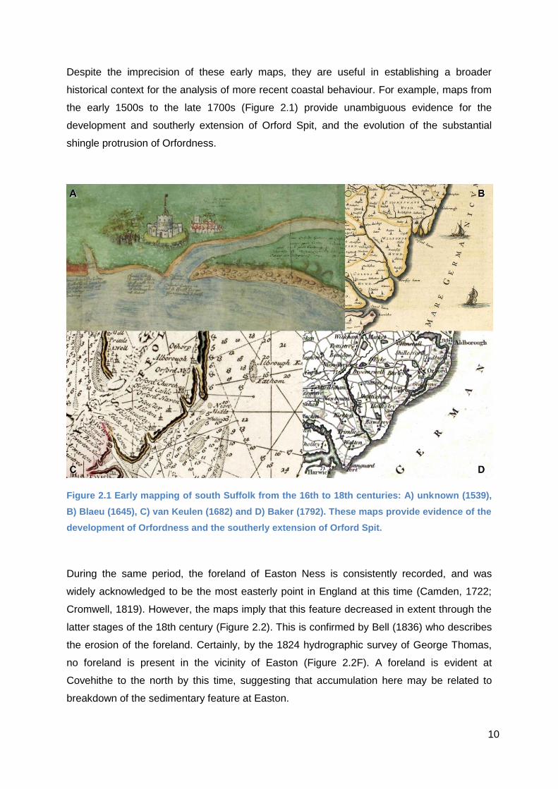
Despite the imprecision of these early maps, they are useful in establishing a broader
historical context for the analysis of more recent coastal behaviour. For example, maps from
the early 1500s to the late 1700s (Figure 2.1) provide unambiguous evidence for the
development and southerly extension of Orford Spit, and the evolution of the substantial
shingle protrusion of Orfordness.
Figure 2.1 Early mapping of south Suffolk from the 16th to 18th centuries: A) unknown (1539),
B) Blaeu (1645), C) van Keulen (1682) and D) Baker (1792). These maps provide evidence of the
development of Orfordness and the southerly extension of Orford Spit.
During the same period, the foreland of Easton Ness is consistently recorded, and was
widely acknowledged to be the most easterly point in England at this time (Camden, 1722;
Cromwell, 1819). However, the maps imply that this feature decreased in extent through the
latter stages of the 18th century (Figure 2.2). This is confirmed by Bell (1836) who describes
the erosion of the foreland. Certainly, by the 1824 hydrographic survey of George Thomas,
no foreland is present in the vicinity of Easton (Figure 2.2F). A foreland is evident at
Covehithe to the north by this time, suggesting that accumulation here may be related to
breakdown of the sedimentary feature at Easton.

11
Figure 2.2 Historical mapping of north Suffolk from the 16th to 18th centuries: A) Saxton
(1575), B) van den Keene (1603), C) van Keulen (1682), D) Morden (1703), E) Bowen (1767) and
F) Thomas (1824).

12
There is no reference to Covehithe Ness before this, and a century later, this shift in place
name is repeated in the change to Benacre Ness, a consequence of the foreland having
moved further north again, to Benacre. It seems likely therefore that essentially the same
foreland feature migrated northward from a position adjacent to Easton Bavents (Burningham
and French, 2014), to a location next to Covehithe (roughly 3 km north of Easton) and more
recently adjacent to Benacre (a further 2.5 km north).
Historical descriptions of the early Easton Ness suggest that it was a more substantial
feature than the Covehithe/Benacre sedimentary forelands (Camden, 1722). The ‘city’ of
Easton Bavents is described as being located on a promontory that extended up to 2 miles
(3.2 km) from the 19th century shoreline. Erosion throughout the 18th and 19th centuries
caused the breakdown of this headland (UKHO, 1869), which presumably provided
significant sediment supply to the adjacent shorelines. One interpretation is that erosion of a
terrestrial foreland (i.e. a lithological structure) was followed by reworking and northerly
transport of a ‘travelling’ sedimentary foreland that is now known as Benacre Ness
(Burningham and French, 2014).
2.1.3 Historical shoreline change
Within a more recent post-1880s time frame, it is possible to determine changes in the
position of well-defined shorelines with reasonable accuracy. The shoreline corresponding to
MHW is consistently mapped and is readily interpreted in terms of recession or progradation
of the coast in general. A summary analysis of the entire set of shorelines acquired for the
1881 to 2013 period is summarised in Figures 2.3 and 2.4. The most dynamic region over
this period lies in the north, between Southwold and Lowestoft. By comparison, the scales of
change along the rest of the Suffolk coastline are much smaller. The geographical pattern of
the envelope of shoreline variability (the Shoreline Change Envelope, or SCE) corresponds
closely with that of the Net Shoreline Movement (NSM). In other words, the variation in the
position of the MHW shoreline at any particular location over the last 130 years or so
correlates strongly with the net shift in shoreline position between 1881 and 2013. This is due
in large part to the consistently high rate of erosion along the main stretches of soft rock cliff;
the NME and SCE are effectively the same for some of these erosion ‘hotspots’. More
generally, it is clear that the SCE is greater for at sites that have experienced net erosion and
than those that have been largely accretional.

13
Figure 2.3 Shoreline change analysis for Suffolk, showing (from left) all shorelines from 1881 to
2013, shoreline change envelope (SCE), linear regression rate of change (LRR), earliest and
most recent shorelines (1880s/2010s), net shoreline movement (NSM) and end point rate of
change (EPR).

14
Figure 2.4 Synthesis of shoreline change (linear regression rate of change (LRR) and end point
rate of change (EPR)) for defined stretches of the Suffolk coast over the period 1881 to 2013.
15
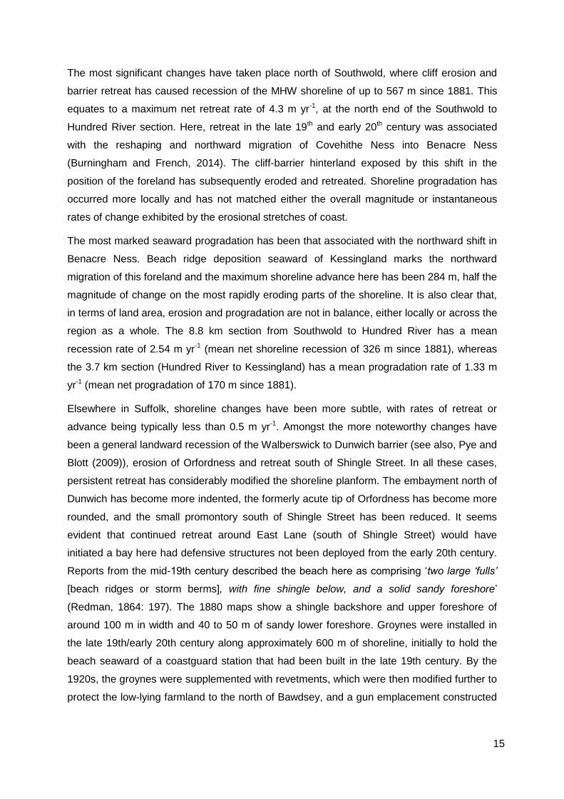
The most significant changes have taken place north of Southwold, where cliff erosion and
barrier retreat has caused recession of the MHW shoreline of up to 567 m since 1881. This
equates to a maximum net retreat rate of 4.3 m yr-1, at the north end of the Southwold to
Hundred River section. Here, retreat in the late 19th and early 20th century was associated
with the reshaping and northward migration of Covehithe Ness into Benacre Ness
(Burningham and French, 2014). The cliff-barrier hinterland exposed by this shift in the
position of the foreland has subsequently eroded and retreated. Shoreline progradation has
occurred more locally and has not matched either the overall magnitude or instantaneous
rates of change exhibited by the erosional stretches of coast.
The most marked seaward progradation has been that associated with the northward shift in
Benacre Ness. Beach ridge deposition seaward of Kessingland marks the northward
migration of this foreland and the maximum shoreline advance here has been 284 m, half the
magnitude of change on the most rapidly eroding parts of the shoreline. It is also clear that,
in terms of land area, erosion and progradation are not in balance, either locally or across the
region as a whole. The 8.8 km section from Southwold to Hundred River has a mean
recession rate of 2.54 m yr-1 (mean net shoreline recession of 326 m since 1881), whereas
the 3.7 km section (Hundred River to Kessingland) has a mean progradation rate of 1.33 m
yr-1 (mean net progradation of 170 m since 1881).
Elsewhere in Suffolk, shoreline changes have been more subtle, with rates of retreat or
advance being typically less than 0.5 m yr-1. Amongst the more noteworthy changes have
been a general landward recession of the Walberswick to Dunwich barrier (see also, Pye and
Blott (2009)), erosion of Orfordness and retreat south of Shingle Street. In all these cases,
persistent retreat has considerably modified the shoreline planform. The embayment north of
Dunwich has become more indented, the formerly acute tip of Orfordness has become more
rounded, and the small promontory south of Shingle Street has been reduced. It seems
evident that continued retreat around East Lane (south of Shingle Street) would have
initiated a bay here had defensive structures not been deployed from the early 20th century.
Reports from the mid-19th century described the beach here as comprising ‘two large ‘fulls’
[beach ridges or storm berms], with fine shingle below, and a solid sandy foreshore’
(Redman, 1864: 197). The 1880 maps show a shingle backshore and upper foreshore of
around 100 m in width and 40 to 50 m of sandy lower foreshore. Groynes were installed in
the late 19th/early 20th century along approximately 600 m of shoreline, initially to hold the
beach seaward of a coastguard station that had been built in the late 19th century. By the
1920s, the groynes were supplemented with revetments, which were then modified further to
protect the low-lying farmland to the north of Bawdsey, and a gun emplacement constructed

16
during WWII (Kelly and Hawkins, 2009). This fixed the shoreline about 80 m landward of its
1880 position.
Over the last 50 years, these defences, and upgrades to them, have maintained the position
of the East Lane shoreline at this location. Modifications have primarily involved maintenance,
and more recently, significant alongshore extension. Around 850 m of the shoreline at East
Lane is currently defended with rock armour, and analysis of the most recent shorelines
show that the low cliffs to the south of East Lane have experienced rapid retreat in recent
years, necessitating responsive modification to the defences (Figure 2.5).
Figure 2.5 A) Recent shoreline change along the cliff line at East Lane (1880s - white stippled
planform/dashed MHW; 2010s - grey planform/solid MHW), and views of the coastal defence
works B) north and C) south of East Lane.
Progradational changes have been very localised, with nothing matching the scale of change
seen at Benacre/Kessingland. Of particular note are the accumulations (and associated
shoreline offsets) to the north of the estuary inlets of the Blyth (south of Southwold), Deben
(south of Shingle Street) and the Stour/Orwell (south of Felixstowe). In the case of the Blyth,
the change in shoreline configuration is marked, where a distinct offset north and south of the

17
inlet has developed due to accretion on the north (Southwold Denes) and erosion on the
south (The Flats, Walberswick) side of a fixed channel (Figure 2.6A). This implies sediment
delivery to the north side, and sediment removal from the south, associated with a net
transport of sediment from north to south.
Figure 2.6 Comparison of the historical (1880s - white stippled planform/dashed MHW) and
recent (2010s - grey planform/solid MHW) sediment barriers at the mouths of A) the Blyth and
B) the Deben estuaries, showing opposing shoreline behaviour north and south of the inlet.
At the Deben inlet, both north (updrift) backshore progradation and south (downdrift) erosion
is evident (Figure 2.6B), but whereas the Blyth tidal inlet is entirely artificially fixed in position,
the Deben inlet is less so, and consequently the ebb tidal delta exhibits considerable
variability over decade-century timescales (Burningham and French, 2006). The difference
here is that there is greater capacity for sediment bypassing (transfer of sediment between
inlet margins) at the Deben than at the Blyth due to the dynamics and extent of ‘The Knolls’
ebb tidal delta. Some interventions have been applied to the shoreline here. North of the inlet
the foreland at Bawdsey Manor is held by sheet piling that was installed in the 1950s, and
further afield, groynes have served a purpose here in the past. To the south, an earth

18
embankment extends along much of the Felixstowe Ferry foreland, protecting the backbarrier
environment, but more recent southwest shifts in the ebb channel have necessitated the on-
going installation of rock armour since the 2001. Sediment accumulation north of the inlet
has likely forced channel movement, and thus erosion of the south margin. But this
behaviour is part of the ebb delta migration cycle that has operated over a 10-30 year period
for at least the last 150 years (Burningham and French, 2006).
The current shoreline position along the Felixstowe Ferry margin is not dissimilar to that of
the 1940-50s (Figure 2.7A); the shoreline had retreated back to this position by 1999,
prompting the initial installation of rock armour toward the south of this stretch (Figure 2.7B).
Several extensions to this armouring have continued since 2001, including some emergency
operations, as the focus of erosion has moved toward the inlet in response to construction.
Figure 2.7 Comparison of shoreline position at the Deben inlet: A) the 2012 shoreline shown
with the 1945/1957 shorelines overlain on all historical shorelines and B) the 1999, 2007 and
2012 shorelines.
Sediment transfer across the inlet does not currently benefit this stretch of the Felixstowe
Ferry shoreline due to the southward extension of the ebb delta shoals, which is where the
19
vast majority of sediment movement occurs. As such, sediment is supplied to the downdrift
shoreline adjacent to Martello Tower T, and the current configuration (ebb channel hugging
the southwest margin) provides little opportunity for transport northward along this shoreline.
The equivalent situation in the 1940-50s was not followed by enhanced erosion of the
Felixstowe Ferry shoreline because the ebb delta underwent significant change in the 1950s.
This was most likely as a result of the 1953 storm surge, which led to breaching of the updrift
shoals (Burningham and French, 2006). This in turn caused repositioning of the ebb channel
to an updrift position with a southeast-directed jet, rather than a downdrift, south-directed jet
that was present in 1950 and 2012 (Figure 2.7). It is unclear whether the application of hard
engineering along this shoreline has interfered with the natural ebb delta cycle, but it seems
that the combination of shoal/channel configuration and a rock-armoured shoreline has
prompted the recent responsive management interventions. Natural alleviation of this
situation is only possible through breaching of the updrift shoal to allow the development of a
foreland to the east of Martello Tower T, and hence provide some capacity for alongshore
supply to Felixstowe Ferry.
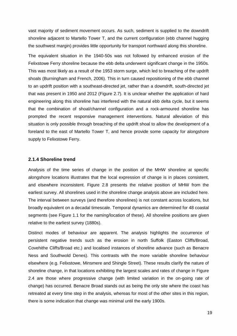
2.1.4 Shoreline trend
Analysis of the time series of change in the position of the MHW shoreline at specific
alongshore locations illustrates that the local expression of change is in places consistent,
and elsewhere inconsistent. Figure 2.8 presents the relative position of MHW from the
earliest survey. All shorelines used in the shoreline change analysis above are included here.
The interval between surveys (and therefore shorelines) is not constant across locations, but
broadly equivalent on a decadal timescale. Temporal dynamics are determined for 48 coastal
segments (see Figure 1.1 for the naming/location of these). All shoreline positions are given
relative to the earliest survey (1880s).
Distinct modes of behaviour are apparent. The analysis highlights the occurrence of
persistent negative trends such as the erosion in north Suffolk (Easton Cliffs/Broad,
Covehithe Cliffs/Broad etc.) and localised instances of shoreline advance (such as Benacre
Ness and Southwold Denes). This contrasts with the more variable shoreline behaviour
elsewhere (e.g. Felixstowe, Minsmere and Shingle Street). These results clarify the nature of
shoreline change, in that locations exhibiting the largest scales and rates of change in Figure
2.4 are those where progressive change (with limited variation in the on-going rate of
change) has occurred. Benacre Broad stands out as being the only site where the coast has
retreated at every time step in the analysis, whereas for most of the other sites in this region,
there is some indication that change was minimal until the early 1900s.

20
Figure 2.8 Relative position of MHW for adjacent shore-normal transect sequences that exhibit
broadly similar styles of behaviour over the period 1881 to 2013 (see Figure 1.1 for location of
sites). Note variable scale of the vertical shoreline position axis.

21
No sites exhibit continuous advance. Rather, some advance and then retreat (e.g. Benacre
Denes) while others retreat and then advance (e.g. Sudbourne Beach). The tendency for the
accretionary stretches to be more temporally variable goes some way to explain the
significantly lower rates of progradational change relative to shoreline recession. Few sites
show clearly stationary behaviour, but some have remained relatively stable throughout the
130-year history (parts of the Bawdsey Cliff, Southwold and Felixstowe stretches). Both
Dunwich and Minsmere Cliffs experienced marked retreat through to the mid-20th century,
but have then stabilised with no significant change since.
When visualised on a common scale, the relative magnitudes of change are very apparent
(Figure 2.9). North of Southwold, both cliff and barrier frontages have shown the same
persistent retreat. This similar behaviour in quite distinct landforms implies that the beach
and nearshore environment, which provide a sediment pathway connecting them, are
determining the scale and direction of change. The magnitude of change here is not found
elsewhere in Suffolk. The progradation at Benacre Ness, and to some extent the dynamics at
Shingle Street, show that significant positive change has also occurred on this coast. Aside
from the above locations, the majority of coastal sites in Suffolk have seen much smaller
changes over the last 130 years.

22
Figure 2.9 As Figure 2.8 relative position of MHW for adjacent shore-normal transect
sequences that exhibit broadly similar styles of behaviour over the period 1881 to 2013, but
with vertical shoreline position axis at a common scale to facilitate inter-site comparison.
23
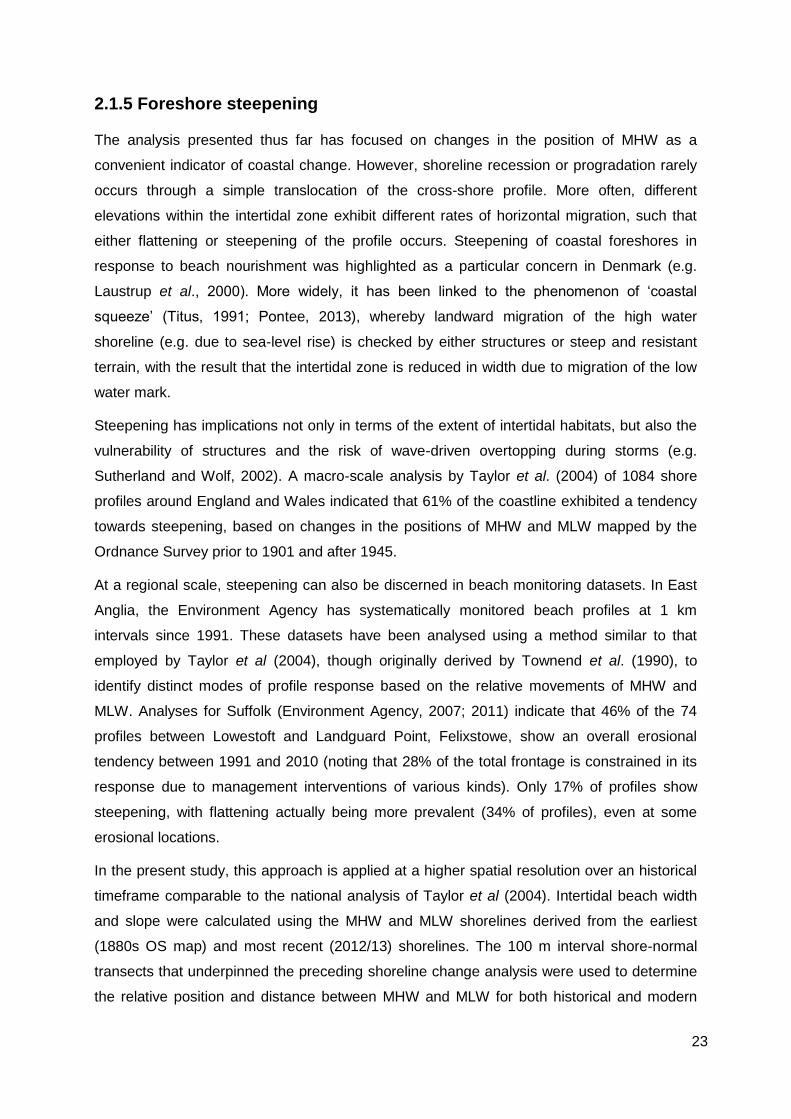
2.1.5 Foreshore steepening
The analysis presented thus far has focused on changes in the position of MHW as a
convenient indicator of coastal change. However, shoreline recession or progradation rarely
occurs through a simple translocation of the cross-shore profile. More often, different
elevations within the intertidal zone exhibit different rates of horizontal migration, such that
either flattening or steepening of the profile occurs. Steepening of coastal foreshores in
response to beach nourishment was highlighted as a particular concern in Denmark (e.g.
Laustrup et al., 2000). More widely, it has been linked to the phenomenon of ‘coastal
squeeze’ (Titus, 1991; Pontee, 2013), whereby landward migration of the high water
shoreline (e.g. due to sea-level rise) is checked by either structures or steep and resistant
terrain, with the result that the intertidal zone is reduced in width due to migration of the low
water mark.
Steepening has implications not only in terms of the extent of intertidal habitats, but also the
vulnerability of structures and the risk of wave-driven overtopping during storms (e.g.
Sutherland and Wolf, 2002). A macro-scale analysis by Taylor et al. (2004) of 1084 shore
profiles around England and Wales indicated that 61% of the coastline exhibited a tendency
towards steepening, based on changes in the positions of MHW and MLW mapped by the
Ordnance Survey prior to 1901 and after 1945.
At a regional scale, steepening can also be discerned in beach monitoring datasets. In East
Anglia, the Environment Agency has systematically monitored beach profiles at 1 km
intervals since 1991. These datasets have been analysed using a method similar to that
employed by Taylor et al (2004), though originally derived by Townend et al. (1990), to
identify distinct modes of profile response based on the relative movements of MHW and
MLW. Analyses for Suffolk (Environment Agency, 2007; 2011) indicate that 46% of the 74
profiles between Lowestoft and Landguard Point, Felixstowe, show an overall erosional
tendency between 1991 and 2010 (noting that 28% of the total frontage is constrained in its
response due to management interventions of various kinds). Only 17% of profiles show
steepening, with flattening actually being more prevalent (34% of profiles), even at some
erosional locations.
In the present study, this approach is applied at a higher spatial resolution over an historical
timeframe comparable to the national analysis of Taylor et al (2004). Intertidal beach width
and slope were calculated using the MHW and MLW shorelines derived from the earliest
(1880s OS map) and most recent (2012/13) shorelines. The 100 m interval shore-normal
transects that underpinned the preceding shoreline change analysis were used to determine
the relative position and distance between MHW and MLW for both historical and modern

24
foreshores. Mean tide range on the Suffolk coast varies from about 2.8 m at Landguard Point
to 1.5 m at Lowestoft (UKHO, 2014). Estimates of the elevation of MHW and MLW were
calculated for each transect based on linear interpolation of predicted tidal levels (relative to
OD) at all the secondary ‘ports’ between Harwich and Lowestoft. Intertidal slopes were thus
calculated from the mean tide range at each transect relative to the intertidal width.
As Figure 2.10 shows, the contemporary intertidal is relatively narrow. The median width is
15.3 m and 79.5% of the shoreline has a width < 20 m. The median beach slope is 6.5° (tan
β = 0.11), with slopes < 5° occurring along only 11.8% of the shoreline. In contrast, the
coast in the 1880s was characterised by wider and flatter beaches (median width and slope
23.0 m and 4.7° (tan β = 0.08) respectively). Only 37.2% of the historical shoreline had a
beach width < 20 m, whilst 60.1% had a beach slope of < 5°. A Kruskal-Wallis
(nonparametric) one-way analysis of variance was significant for both width and slope,
indicating a significant difference in modern and historical values (width χ2 = 480.66, p <
0.001; slope χ2 = 440, p < 0.001).
Figure 2.10 Comparison of modern (2010s) and historical (1880s) intertidal beach width and
slope for Suffolk.
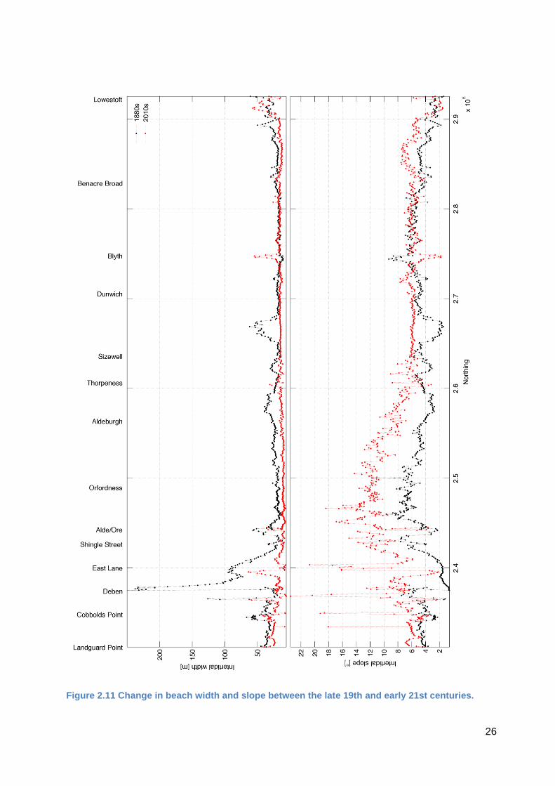
Intertidal morphology is quite variable, with distinct stretches of shoreline exhibiting
significantly wider (or shallower) foreshores (Figure 2.11). Local increases in intertidal width
(and flatter beach gradients) are found just south of East Lane (north of Bawdsey), at
Walberswick (south of the Blyth inlet) and South Beach (Lowestoft). The beach at East Lane

25
was also wide in the late 19th century, but the extreme widths illustrated around the Deben
reflect the configuration of the ebb tidal delta shoals at that time, and are not comparable to
the localised widening of beaches seen at other locations. Elsewhere, the 1880s foreshore
exhibited greater alongshore variation in beach width, as well as stretches of wider beach
between Aldeburgh and Thorpeness, between Sizewell and Dunwich, and near Pakefield
Cliffs. Both the mid-Suffolk sites are associated with barrier systems that front backbarrier
marshes and lagoons, where the interplay between barrier and wetland has the potential to
be more dynamic than where a beach is backed by a cliff. Between Aldeburgh and
Thorpeness lies The Haven, and between Sizewell and Dunwich lies Minsmere. Evidence
from the 1880s OS maps suggests that these wetlands were more extensive and that the
barrier fronting them was generally broader 130 years ago, implying that changes to the
wetlands (and their management) might be responsible for the significant reduction in
intertidal width at these locations.
Somewhat contrary to the findings that emerge from the last two decades of surveyed beach
profiles (EA, 2007, 2011), the centennial-scale picture in Suffolk coast is one of decreasing
beach widths and increasing foreshore slope. As already noted, a similar historical
steepening trend has been reported for England and Wales as a whole, based on the
analysis of a much sparser set of otherwise similarly derived profiles (Taylor et al., 2004).
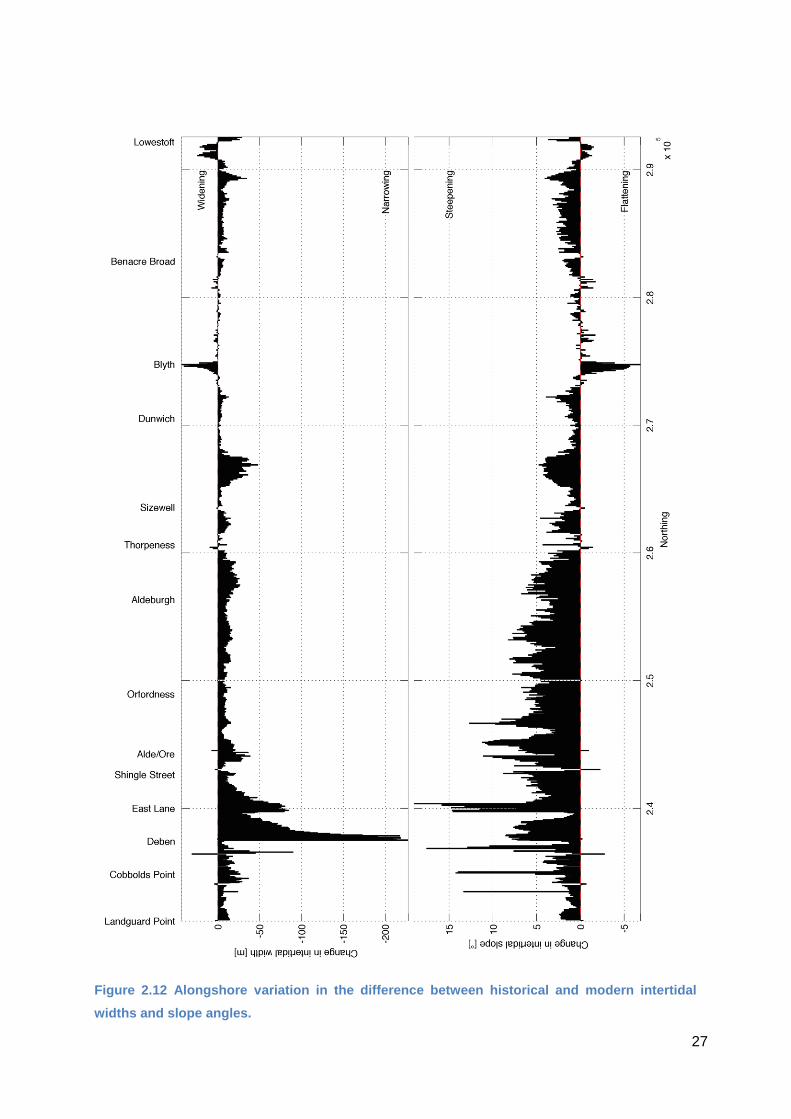
The present analysis shows that 89% of the Suffolk coast has experienced a reduction in
beach width since the late 19th century. Taylor et al. (2004) found that 64% of east coast
profiles experienced steepening over this same period. Suffolk has thus seen more
widespread steepening than the east coast in general. The few sites that show broadening of
the intertidal profile are those associated with South Beach (Lowestoft) and shorelines either
side of the Blyth inlet (Figure 2.12). Analysis of beach profiles between 1992 and 2010
corroborates the accretion and profile flattening at South Beach, but also reveal strong
summer to winter and multi-annual shifts in profile morphology (EA, 2011).
Foreshore flattening is particularly pronounced at Walberswick (Town Salts and The Flats)
and Southwold Denes, to the north and south of the Blyth inlet. Over the last century, inlet
stability structures have increasingly forced a significant offset in position of the barrier
shorelines here (Figure 2.6A). Accretion to the north of the inlet has advanced the shoreline,
whilst the Walberswick shoreline has retreated. Although there is no obvious reason why this
should result in a shallower intertidal profile, it is possible that the presence of the jetties and
the resulting shoreline offset has afforded a degree of shelter to the beaches immediately
north and south of the inlet.
26
Figure 2.11 Change in beach width and slope between the late 19th and early 21st centuries.
27
Figure 2.12 Alongshore variation in the difference between historical and modern intertidal
widths and slope angles.
28
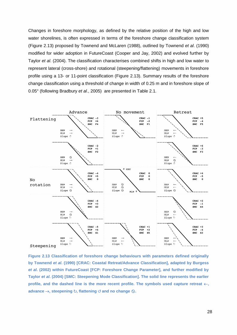
Changes in foreshore morphology, as defined by the relative position of the high and low
water shorelines, is often expressed in terms of the foreshore change classification system
(Figure 2.13) proposed by Townend and McLaren (1988), outlined by Townend et al. (1990)
modified for wider adoption in FutureCoast (Cooper and Jay, 2002) and evolved further by
Taylor et al. (2004). The classification characterises combined shifts in high and low water to
represent lateral (cross-shore) and rotational (steepening/flattening) movements in foreshore
profile using a 13- or 11-point classification (Figure 2.13). Summary results of the foreshore
change classification using a threshold of change in width of 0.25 m and in foreshore slope of
0.05° (following Bradbury et al., 2005) are presented in Table 2.1.
Figure 2.13 Classification of foreshore change behaviours with parameters defined originally
by Townend et al. (1990) [CRAC: Coastal Retreat/Advance Classification], adapted by Burgess
et al. (2002) within FutureCoast [FCP: Foreshore Change Parameter], and further modified by
Taylor et al. (2004) [SMC: Steepening Mode Classification]. The solid line represents the earlier
profile, and the dashed line is the more recent profile. The symbols used capture retreat ,
advance , steepening ↻, flattening ↺ and no change .

29
Application of this approach to the Suffolk coast at a centennial scale (1880s to 2010s)
reveals that the broad picture of steepening and retreat is more complex when a wider suite
of foreshore behaviours is considered. The results are presented in the context of both the
Foreshore Change Parameter and the Steepening Mode Classification. Almost half the
Suffolk coast is retreating and steepening (FCP -6). In the Taylor et al. (2004) national
analysis, this mode (S3) - where retreat is evident in both the low and high water shorelines,
but experienced at a higher rate in the high water shoreline - was observed along 23% of the
coastline of England and Wales, but the S5 mode of steepening (advance in MHW and
retreat in MLW) was equally dominant. In the present Suffolk analysis, S5 (FCP +2) is
evident along just 9% of the shoreline. Where advance is taking place along the Suffolk
MHW, it is more frequently associated with an advance in the MLW, but at a reduced rate.
This still leads to overall steepening of the foreshore (S1; FCP +4). Foreshore flattening is
rare, and is predominately associated with higher rates of retreat of MHW than of MLW.
Table 2.1 Summary of net foreshore behaviour in Suffolk (1880s to 2010s). Mode refers to the
Foreshore Change Parameter and [Steepening Mode Classification] (see Figure 2.13).
Net advance No net movement Net retreat
Mode % Mode % Mode % Total
Flattening +6 [F4] 3.4% -2 [F1] 0.3% -4 [F5] 7.2% 10.9%
+1 [F2] 0% -3 [F3] 0%
No rotation +5 [0] 0.5% 0 [0] 0 -5 [0] 0.4% 0.9%
+3 [S2] 0.3% -1 [S4] 0.3%
Steepening +4 [S1] 29.4% +2 [S5] 8.8% -6 [S3] 49.4% 88.2%
Total 33.6% 9.1% 57.3%
The role of different backshore contexts on foreshore behaviour modes was also examined.
Each of the 100 m interval shore-normal transects was assessed for the presence of coastal
defences (e.g. sea wall, revetment), cliff backed by higher ground and beach ridge/barrier
backshore sedimentary system. Comparison of the frequency distributions of these different
contexts shows that the dominant modes of behaviour consistently dominate across all
backshore contexts (Figure 2.14). Irrespective of whether the backshore is defended,
erosional or depositional, S3 / FCP -6 (retreat of both shorelines, but at a faster rate for MLW
relative to MHW, leading to steepening) is the most common mode of profile behaviour.

30
A
B
Figure 2.14 Frequency distributions of different modes of foreshore behaviour: A) Foreshore
Change Parameter and B) Steepening Mode Classification in the context of different backshore
types (defended, cliff and beach ridge/barrier). Transparent bars show the distribution across
all backshore types in Suffolk.
31
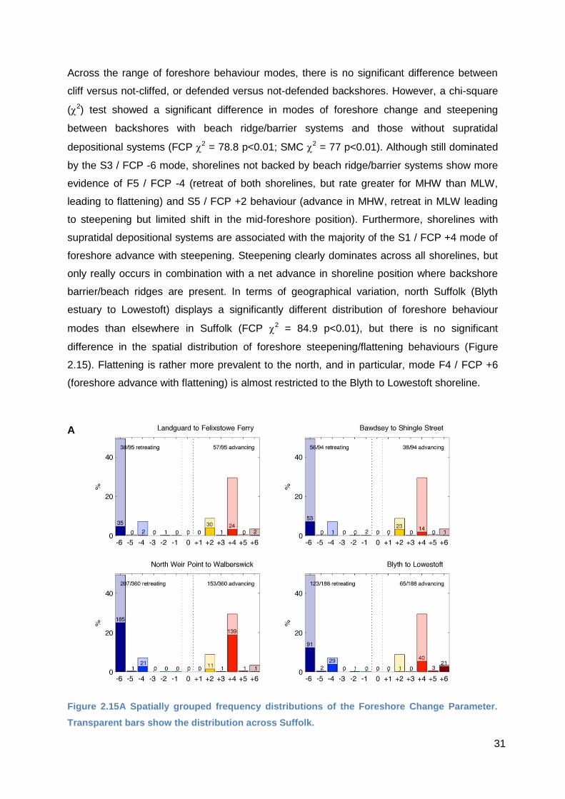
Across the range of foreshore behaviour modes, there is no significant difference between
cliff versus not-cliffed, or defended versus not-defended backshores. However, a chi-square
(2) test showed a significant difference in modes of foreshore change and steepening
between backshores with beach ridge/barrier systems and those without supratidal
depositional systems (FCP 2 = 78.8 p<0.01; SMC 2 = 77 p<0.01). Although still dominated
by the S3 / FCP -6 mode, shorelines not backed by beach ridge/barrier systems show more
evidence of F5 / FCP -4 (retreat of both shorelines, but rate greater for MHW than MLW,
leading to flattening) and S5 / FCP +2 behaviour (advance in MHW, retreat in MLW leading
to steepening but limited shift in the mid-foreshore position). Furthermore, shorelines with
supratidal depositional systems are associated with the majority of the S1 / FCP +4 mode of
foreshore advance with steepening. Steepening clearly dominates across all shorelines, but
only really occurs in combination with a net advance in shoreline position where backshore
barrier/beach ridges are present. In terms of geographical variation, north Suffolk (Blyth
estuary to Lowestoft) displays a significantly different distribution of foreshore behaviour
modes than elsewhere in Suffolk (FCP 2 = 84.9 p<0.01), but there is no significant
difference in the spatial distribution of foreshore steepening/flattening behaviours (Figure
2.15). Flattening is rather more prevalent to the north, and in particular, mode F4 / FCP +6
(foreshore advance with flattening) is almost restricted to the Blyth to Lowestoft shoreline.
A
Figure 2.15A Spatially grouped frequency distributions of the Foreshore Change Parameter.
Transparent bars show the distribution across Suffolk.

32
B
Figure 2.15B Spatially grouped frequency distributions of the Steepening Mode Classification.
Transparent bars show the distribution across Suffolk.
2.1.6 Classification of coastal behaviour
Classification of historical coastal behaviour was undertaken using a cluster analysis of
historical shoreline positions. All shoreline data are measured in the same units relative to a
consistent baseline, so transformation of these data was not necessary. However, some
collation of data was required due to the variability in shoreline dates. Epochs were derived
that broadly matched the temporal sequence and availability of data, and within each of
these epochs (1881-1900; 1901-1950; 1951-1970; 1971-1990; 1991-2000; 2001-2007; 2008-
2013), shoreline positions (if more than one survey contributed to a specific epoch) were
averaged. A small number of transects (primarily in the region of estuary mouths) were
removed due to lack of data. The resulting dataset extends over 730 locations and 7 epochs.
Hierarchical cluster analysis was applied to the data to derive groupings of locations
exhibiting similar shoreline behaviour. Cluster analysis involves the calculations of distances
between all objects in the data matrix, on the basis that those closer together are more alike
that those further apart. Here, the Euclidean distance and average linkage were used. This
resulted in a cophenetic correlation coefficient (which reflects the accuracy of the clustering)
of 0.75 to 0.85 (on the scale of 0 to 1, with 1 representing a perfect correlation).

33
Results of the analysis suggested that 3 clusters best represent the full dataset. The
shoreline statistics associated with this primary classification are provided in Figure 2.16A.
This clustering shows that scale and direction of change are the main distinguishing
attributes of coastal behaviour; differences in scale of coastal change (cluster 1 - small;
cluster 2 - medium; cluster 3 - large), in addition to direction of change (cluster 1 - retreat and
advance; cluster 2 - advance; cluster 3 - retreat). It is clear though, that cluster 1 comprises a
large proportion of the shoreline with some degree of spread in some of the shoreline change
parameters. Clusters 2 and 3 more effectively distinguish clear stretches of coast exhibiting
very similar behaviour (Figure 2.16B).
A
B
Figure 2.16 A) Shoreline change parameters associated with the 3 primary ‘types’ of shoreline
behaviour identified through the application of cluster analysis and B) alongshore
classification of transects using this typology.
34
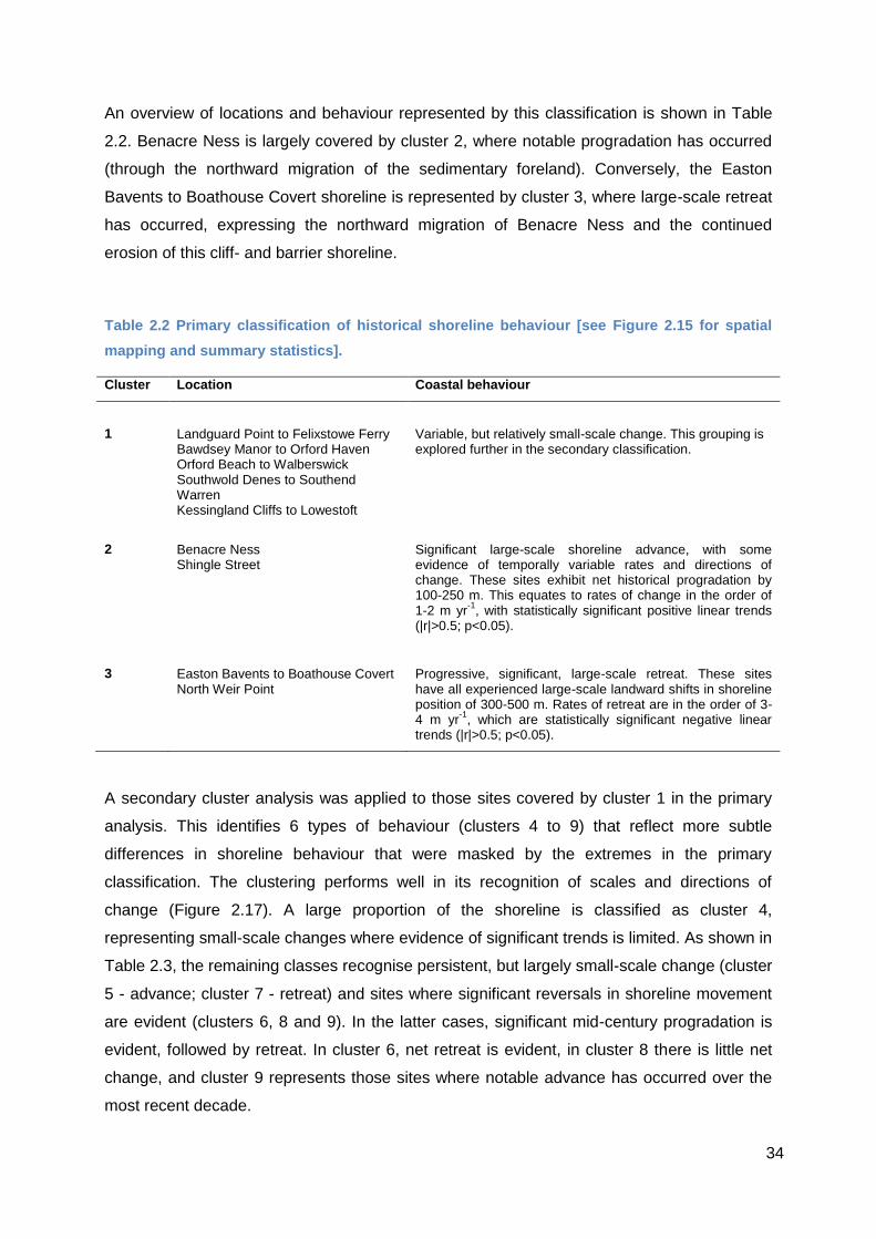
An overview of locations and behaviour represented by this classification is shown in Table
2.2. Benacre Ness is largely covered by cluster 2, where notable progradation has occurred
(through the northward migration of the sedimentary foreland). Conversely, the Easton
Bavents to Boathouse Covert shoreline is represented by cluster 3, where large-scale retreat
has occurred, expressing the northward migration of Benacre Ness and the continued
erosion of this cliff- and barrier shoreline.
Table 2.2 Primary classification of historical shoreline behaviour [see Figure 2.15 for spatial
mapping and summary statistics].
Cluster Location Coastal behaviour
1 Landguard Point to Felixstowe Ferry Bawdsey Manor to Orford Haven Orford Beach to Walberswick Southwold Denes to Southend Warren Kessingland Cliffs to Lowestoft
Variable, but relatively small-scale change. This grouping is explored further in the secondary classification.
2 Benacre Ness Shingle Street
Significant large-scale shoreline advance, with some evidence of temporally variable rates and directions of change. These sites exhibit net historical progradation by 100-250 m. This equates to rates of change in the order of 1-2 m yr
-1, with statistically significant positive linear trends
(|r|>0.5; p<0.05).
3 Easton Bavents to Boathouse Covert North Weir Point
Progressive, significant, large-scale retreat. These sites have all experienced large-scale landward shifts in shoreline position of 300-500 m. Rates of retreat are in the order of 3-4 m yr
-1, which are statistically significant negative linear
trends (|r|>0.5; p<0.05).
A secondary cluster analysis was applied to those sites covered by cluster 1 in the primary
analysis. This identifies 6 types of behaviour (clusters 4 to 9) that reflect more subtle
differences in shoreline behaviour that were masked by the extremes in the primary
classification. The clustering performs well in its recognition of scales and directions of
change (Figure 2.17). A large proportion of the shoreline is classified as cluster 4,
representing small-scale changes where evidence of significant trends is limited. As shown in
Table 2.3, the remaining classes recognise persistent, but largely small-scale change (cluster
5 - advance; cluster 7 - retreat) and sites where significant reversals in shoreline movement
are evident (clusters 6, 8 and 9). In the latter cases, significant mid-century progradation is
evident, followed by retreat. In cluster 6, net retreat is evident, in cluster 8 there is little net
change, and cluster 9 represents those sites where notable advance has occurred over the
most recent decade.

35
This analysis reveals the distinctiveness of coastal change in north Suffolk. The rates of
retreat experienced along the Easton Bavents to Boathouse Covert shoreline are within the
ranges quoted for the Holderness (East Riding) and Lincolnshire coasts (Quinn et al., 2009;
Montreuil and Bullard, 2012). In Suffolk, however, this stretch of exceptional erosion is
adjacent to a foreland environment that has advanced the coastline by hundreds of metres.
As noted earlier, these stretches of retreat and advance are not balanced, with retreat out-
pacing advance.
A
B
Figure 2.17 A) Shoreline change parameters associated with the 6 secondary ‘types’ of
shoreline behaviour identified through the application of cluster analysis and B) alongshore
classification of transects using this typology.
36
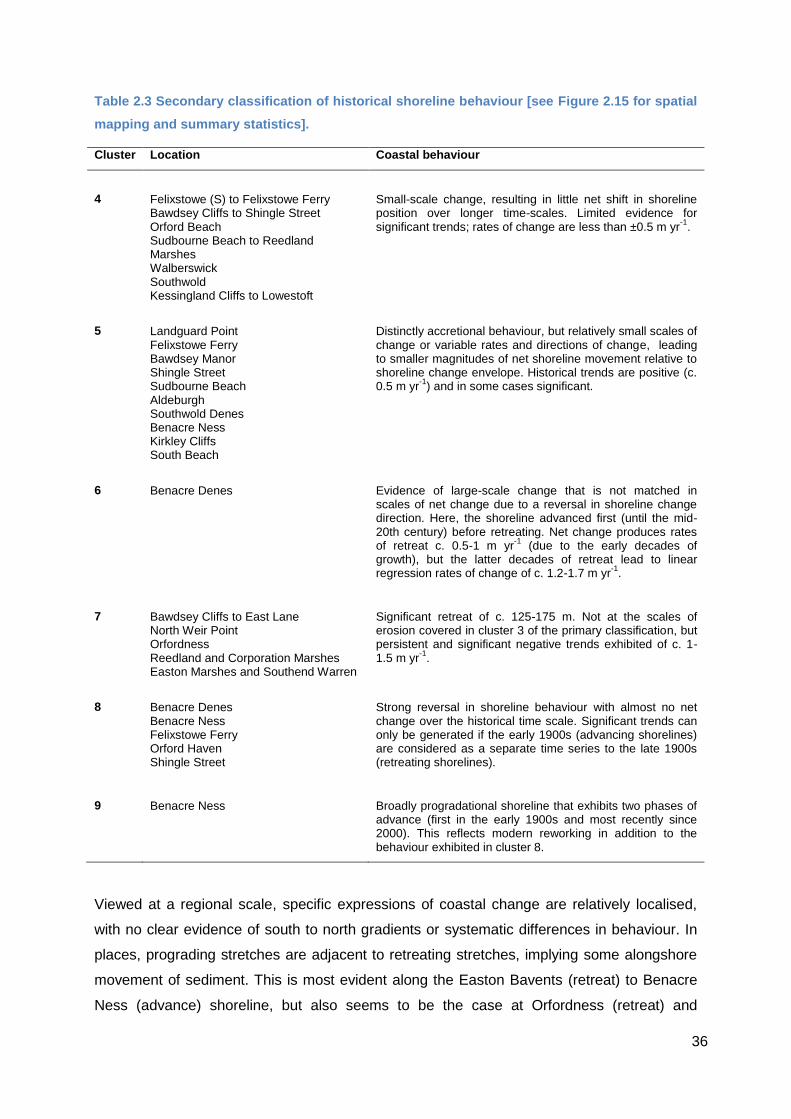
Table 2.3 Secondary classification of historical shoreline behaviour [see Figure 2.15 for spatial
mapping and summary statistics].
Cluster Location Coastal behaviour
4 Felixstowe (S) to Felixstowe Ferry Bawdsey Cliffs to Shingle Street Orford Beach Sudbourne Beach to Reedland Marshes Walberswick Southwold Kessingland Cliffs to Lowestoft
Small-scale change, resulting in little net shift in shoreline position over longer time-scales. Limited evidence for significant trends; rates of change are less than ±0.5 m yr
-1.
5 Landguard Point Felixstowe Ferry Bawdsey Manor Shingle Street Sudbourne Beach Aldeburgh Southwold Denes Benacre Ness Kirkley Cliffs South Beach
Distinctly accretional behaviour, but relatively small scales of change or variable rates and directions of change, leading to smaller magnitudes of net shoreline movement relative to shoreline change envelope. Historical trends are positive (c. 0.5 m yr
-1) and in some cases significant.
6 Benacre Denes Evidence of large-scale change that is not matched in scales of net change due to a reversal in shoreline change direction. Here, the shoreline advanced first (until the mid-20th century) before retreating. Net change produces rates of retreat c. 0.5-1 m yr
-1 (due to the early decades of
growth), but the latter decades of retreat lead to linear regression rates of change of c. 1.2-1.7 m yr
-1.
7 Bawdsey Cliffs to East Lane North Weir Point Orfordness Reedland and Corporation Marshes Easton Marshes and Southend Warren
Significant retreat of c. 125-175 m. Not at the scales of erosion covered in cluster 3 of the primary classification, but persistent and significant negative trends exhibited of c. 1-1.5 m yr
-1.
8 Benacre Denes Benacre Ness Felixstowe Ferry Orford Haven Shingle Street
Strong reversal in shoreline behaviour with almost no net change over the historical time scale. Significant trends can only be generated if the early 1900s (advancing shorelines) are considered as a separate time series to the late 1900s (retreating shorelines).
9 Benacre Ness Broadly progradational shoreline that exhibits two phases of advance (first in the early 1900s and most recently since 2000). This reflects modern reworking in addition to the behaviour exhibited in cluster 8.
Viewed at a regional scale, specific expressions of coastal change are relatively localised,
with no clear evidence of south to north gradients or systematic differences in behaviour. In
places, prograding stretches are adjacent to retreating stretches, implying some alongshore
movement of sediment. This is most evident along the Easton Bavents (retreat) to Benacre
Ness (advance) shoreline, but also seems to be the case at Orfordness (retreat) and
37
Sudbourne Beach to the north (advance). This is not occurring consistently or frequently
enough to suggest regional-scale alongshore ‘pulsing’ of sediment, but these localised
sections of consistent behaviour have led to a distinct net change in regional shoreline
planform over the last century. This is also apparent around some estuary mouths, where
small-scale, significant advance has preferentially occurred on the northern margin of the
inlet. This is the case at Southwold Denes (north of the Blyth), Bawdsey Manor (north of the
Deben) and Landguard Point (north of the Stour/Orwell). Interestingly, the Alde/Ore inlet
displays the opposite trend, where progradation has occurred at Shingle Street (south of the
inlet), and North Weir Point has shown largely erosional behaviour over the last 130 years.
Significant reversals in shoreline behaviour are evident in a few locations (Benacre Ness,
Shingle Street, Felixstowe Ferry). In all cases, these reflect shoreline advance during the first
half of the 20th century, reaching a seaward maxima between 1930 and 1960, followed by
retreat through to the most recent decade. In some cases, renewed advance is evident
during this last decade. Cyclical shoreline behaviour is often overlooked, as the net rates of
change can be relatively small. However, the cluster analysis undertaken here very
effectively resolves situations where small rates of change are not entirely reflective of
reduced dynamics. Here, the reversals are a consequence of the alongshore migration of a
sedimentary foreland (of varying sizes). At Shingle Street and Felixstowe Ferry, the presence
and movement of foreshore accumulations are inherently linked to inlet dynamics. Channel
and ebb shoal migration leads to cycles of enhanced recession of the downdrift margin
followed by growth as the channel moves across the inlet zone before breaching back to an
updrift position (Burningham and French, 2007). At Benacre Ness, however, the cycles of
advance/retreat are the consequence of a sedimentary foreland migrating northwards along
a largely receding shoreline (Burningham and French, 2014).
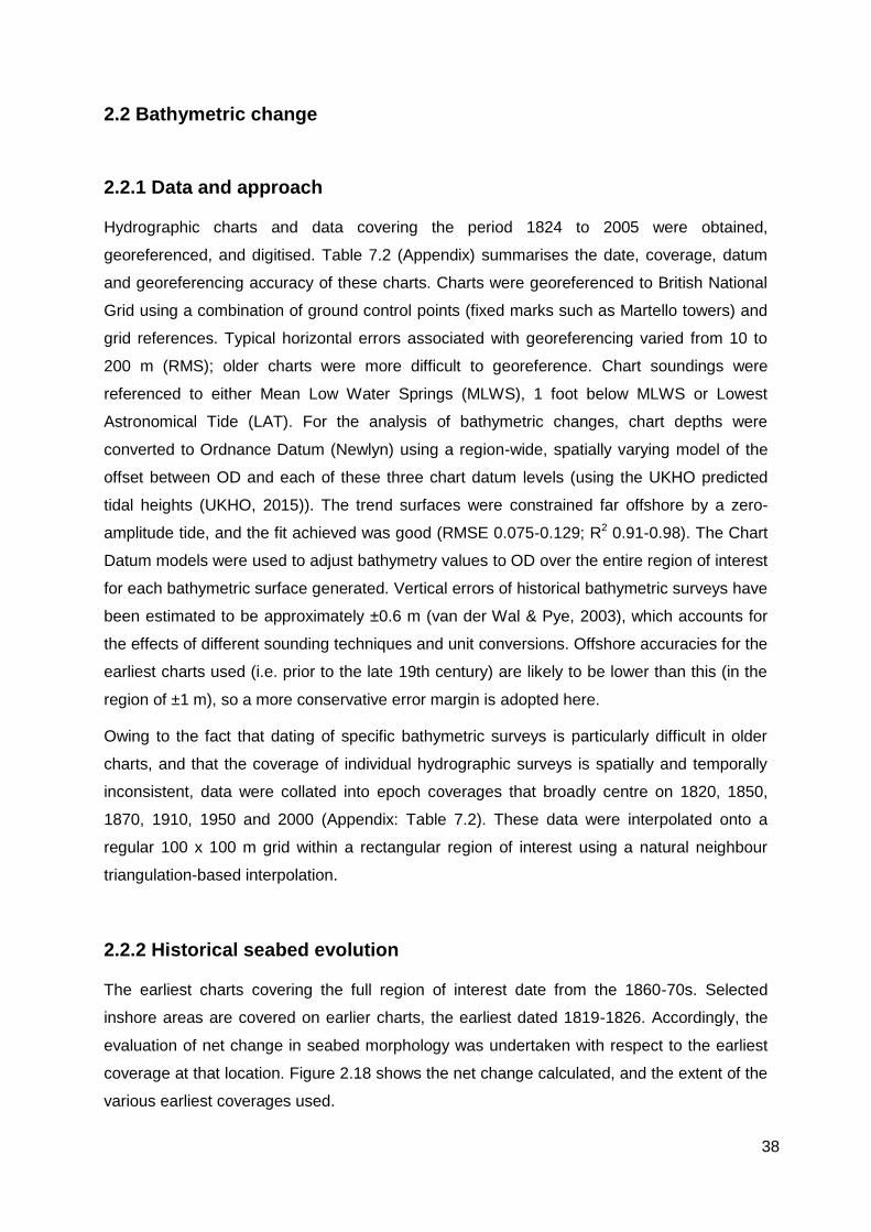
38
2.2 Bathymetric change
2.2.1 Data and approach
Hydrographic charts and data covering the period 1824 to 2005 were obtained,
georeferenced, and digitised. Table 7.2 (Appendix) summarises the date, coverage, datum
and georeferencing accuracy of these charts. Charts were georeferenced to British National
Grid using a combination of ground control points (fixed marks such as Martello towers) and
grid references. Typical horizontal errors associated with georeferencing varied from 10 to
200 m (RMS); older charts were more difficult to georeference. Chart soundings were
referenced to either Mean Low Water Springs (MLWS), 1 foot below MLWS or Lowest
Astronomical Tide (LAT). For the analysis of bathymetric changes, chart depths were
converted to Ordnance Datum (Newlyn) using a region-wide, spatially varying model of the
offset between OD and each of these three chart datum levels (using the UKHO predicted
tidal heights (UKHO, 2015)). The trend surfaces were constrained far offshore by a zero-
amplitude tide, and the fit achieved was good (RMSE 0.075-0.129; R2 0.91-0.98). The Chart
Datum models were used to adjust bathymetry values to OD over the entire region of interest
for each bathymetric surface generated. Vertical errors of historical bathymetric surveys have
been estimated to be approximately ±0.6 m (van der Wal & Pye, 2003), which accounts for
the effects of different sounding techniques and unit conversions. Offshore accuracies for the
earliest charts used (i.e. prior to the late 19th century) are likely to be lower than this (in the
region of ±1 m), so a more conservative error margin is adopted here.
Owing to the fact that dating of specific bathymetric surveys is particularly difficult in older
charts, and that the coverage of individual hydrographic surveys is spatially and temporally
inconsistent, data were collated into epoch coverages that broadly centre on 1820, 1850,
1870, 1910, 1950 and 2000 (Appendix: Table 7.2). These data were interpolated onto a
regular 100 x 100 m grid within a rectangular region of interest using a natural neighbour
triangulation-based interpolation.
2.2.2 Historical seabed evolution
The earliest charts covering the full region of interest date from the 1860-70s. Selected
inshore areas are covered on earlier charts, the earliest dated 1819-1826. Accordingly, the
evaluation of net change in seabed morphology was undertaken with respect to the earliest
coverage at that location. Figure 2.18 shows the net change calculated, and the extent of the
various earliest coverages used.
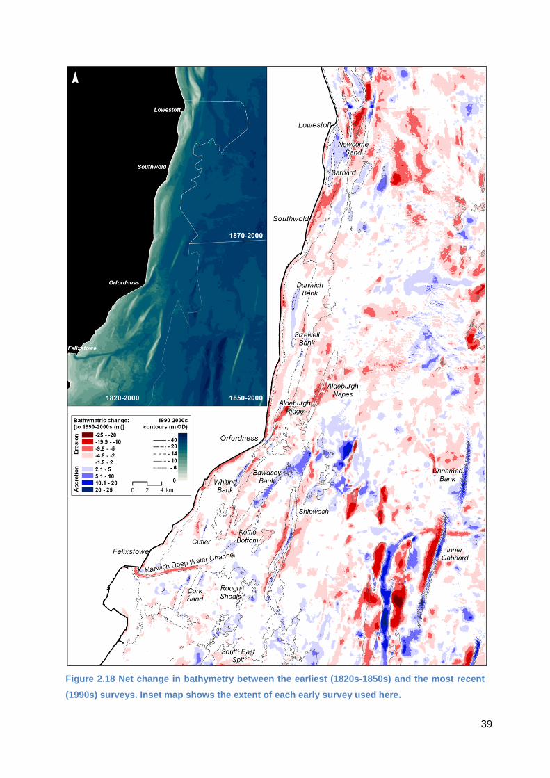
39
Figure 2.18 Net change in bathymetry between the earliest (1820s-1850s) and the most recent
(1990s) surveys. Inset map shows the extent of each early survey used here.

40
It is clear from Figure 2.18 that the seabed across the region has experienced both net
accretion and erosion, and that the scale and pattern of these changes is spatially variable.
The greatest magnitudes of change are centred on the southeast (between Shipwash and
the Inner Gabbard) and north (north and east of Newcome Sand). In the southeast, coarse
survey resolution can perhaps explain some of the change observed, especially since the full
extent of deep areas is not always well represented on older charts. Neighbouring elongated
patches of erosion and accretion usually imply cross-shoreface movement of large-scale
bedforms or banks. But the case west of Inner Gabbard suggests the deepening of two long
channels separated by an accreting ridge. On examination of the original historical charts, it
is clear that this area comprises a mix of shallower and deeper soundings, but that the
resolution of the surveys was probably insufficient to capture the elongated structure of these
entrenched features, and in particular the narrow ridge between them (Figure 2.19).
Positioning errors can also cause these lateral shift characteristics, but in this case, these
errors are not large enough to account for the changes shown. Depths describing the deep
trenches and central ridge are evident in the 1842 chart (overlaid on the modern bathymetry
in Figure 2.19), but there are only a few shallow points describing the ridge. This is thus
represented as a more subdued feature than it appears on more recent surveys. What is
interesting, though, in this comparison is the presence of many shallower depth soundings,
and a contour line across the middle of the eastern trench. As several data points exist here,
and a contour has been used to depict the shape of the feature, it seems likely that the
trench was rather less continuous in the mid-19th century than it is today.
Large areas of seabed exhibit small-scale changes (< ±2 m) interspersed with more
significant change. In many cases, the more significant changes are found within the vicinity
of bank features. To the north of Inner Gabbard, an unnamed bank (which comprises an
extended, but elongated area of sand waves) shows as a region of positive change (seabed
accretion). However, this feature does not appear on any early charts, as established in
previous studies (Burningham and French, 2009), and it is not clear if this is a consequence
of recent formation or lack of survey effort, particularly given the dynamic and variable
morphology associated with sand wave areas. As expected, Harwich Deep Water Channel
contributes a distinctive erosional signature (dredging of this ship channel did not start until
the second half of the 20th century) within a broader area of small scale change. The seabed
around Shipwash has lowered, but the bank itself shows some accretion, possibly the result
of reworking where erosion along the bank margins has supplied sediment for accretion
along the bank top. Bawdsey Bank has also accreted, but over a more substantial area,
including a large region to the north of the bank. This is linked to the hairpin structure that
Bawdsey Bank and Shipwash form in combination, likely associated with the opposing ebb

41
(north-flowing, between the banks) and flood (south-flowing, around the banks) tidal currents.
Here, substantial accretion within the north part of this system and erosion to the south has
resulted in the northward shift of the whole system.
Figure 2.19 The 1842 chart data overlaid on modern bathymetry in the region of Inner Gabbard.
Further north, erosion dominates around Aldeburgh Napes, which has been considerably
reduced in size, and further north, seaward of Sizewell and Dunwich banks. The erosional
trend continues within the Barnard-Newcome system, where the Barnard shoal has shifted
northward (linked to the northward migration of Benacre Ness), and Newcome Sand seems
to have moved landward. Further offshore, there are large areas of erosion, but none linked
to specific morphological features. In addition to this broad picture of deepening, there is a
clear indication of erosion along almost the entire Suffolk nearshore. This supports the
finding that most of the Suffolk foreshore has experienced narrowing and steepening (section
2.15).
Bank migration is evident at several sites where bank-shaped accretion patterns are found
adjacent to erosional patterns. Clear offshore bank migration has only occurred at Cutler
(south Suffolk), where the bank has shifted approximately 1 km to the east and rotated
clockwise by about 5°. Most of the banks show onshore migration. The northward shift at
Bawdsey Bank has moved it closer to the Orfordness shoreline, whilst Whiting Bank and
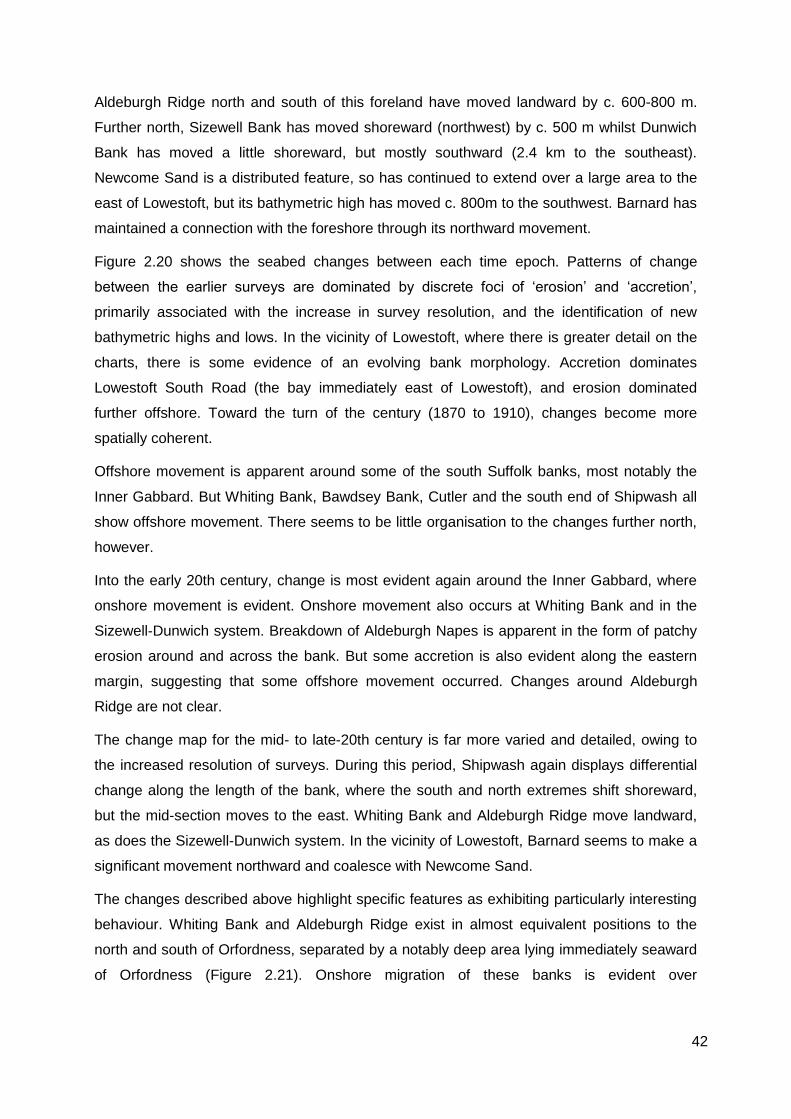
42
Aldeburgh Ridge north and south of this foreland have moved landward by c. 600-800 m.
Further north, Sizewell Bank has moved shoreward (northwest) by c. 500 m whilst Dunwich
Bank has moved a little shoreward, but mostly southward (2.4 km to the southeast).
Newcome Sand is a distributed feature, so has continued to extend over a large area to the
east of Lowestoft, but its bathymetric high has moved c. 800m to the southwest. Barnard has
maintained a connection with the foreshore through its northward movement.
Figure 2.20 shows the seabed changes between each time epoch. Patterns of change
between the earlier surveys are dominated by discrete foci of ‘erosion’ and ‘accretion’,
primarily associated with the increase in survey resolution, and the identification of new
bathymetric highs and lows. In the vicinity of Lowestoft, where there is greater detail on the
charts, there is some evidence of an evolving bank morphology. Accretion dominates
Lowestoft South Road (the bay immediately east of Lowestoft), and erosion dominated
further offshore. Toward the turn of the century (1870 to 1910), changes become more
spatially coherent.
Offshore movement is apparent around some of the south Suffolk banks, most notably the
Inner Gabbard. But Whiting Bank, Bawdsey Bank, Cutler and the south end of Shipwash all
show offshore movement. There seems to be little organisation to the changes further north,
however.
Into the early 20th century, change is most evident again around the Inner Gabbard, where
onshore movement is evident. Onshore movement also occurs at Whiting Bank and in the
Sizewell-Dunwich system. Breakdown of Aldeburgh Napes is apparent in the form of patchy
erosion around and across the bank. But some accretion is also evident along the eastern
margin, suggesting that some offshore movement occurred. Changes around Aldeburgh
Ridge are not clear.
The change map for the mid- to late-20th century is far more varied and detailed, owing to
the increased resolution of surveys. During this period, Shipwash again displays differential
change along the length of the bank, where the south and north extremes shift shoreward,
but the mid-section moves to the east. Whiting Bank and Aldeburgh Ridge move landward,
as does the Sizewell-Dunwich system. In the vicinity of Lowestoft, Barnard seems to make a
significant movement northward and coalesce with Newcome Sand.
The changes described above highlight specific features as exhibiting particularly interesting
behaviour. Whiting Bank and Aldeburgh Ridge exist in almost equivalent positions to the
north and south of Orfordness, separated by a notably deep area lying immediately seaward
of Orfordness (Figure 2.21). Onshore migration of these banks is evident over

43
Figure 2.20 Sequential bathymetric change of the Suffolk shoreface since the early 1800s.

44
the last 150-180 years, with an average movement of around 3-5 m yr-1. Whiting Bank
appears to show more continuous, progressive movement, whereas Aldeburgh Ridge was
more active in the late 19th and 20th centuries but less active between these periods. There
is also some suggestion that the intervening deep area has also moved shoreward over this
time. The shoreline change analysis (Section 2.1) showed that Orfordness has experienced
more-or-less progressive historical retreat, leading to the reshaping of this foreland;
Sudbourne Beach to the north has experienced accretion and Orford Beach shows stability.
The onshore movement of the Aldeburgh Ridge - Whiting Bank system seems to have
afforded protection to (and led to stability or even accumulation of) the beaches north and
south of Orfordness, whilst the continued presence of the deep area immediately seaward
(and some onshore movement) has possibly increased wave focusing on (and hence erosion
of) the foreland.
Further north, seabed evolution in the vicinity of the Sizewell-Dunwich Bank system can also
be linked to historical shoreline change. In the early 19th century, these banks were separate
features that were semi-connected at their southerly extent, Sizewell Bank at Thorpeness
and to a lesser extent, Dunwich Bank just south of Dunwich (Figure 2.22). At that time, the
Minsmere-Dunwich Cliffs were protected from waves to the northeast by the Dunwich Bank,
but exposed to the southeast.
By the late 1800s, the banks had partly coalesced, a process that has continued since.
Throughout the history considered here, the southern extent of Sizewell Bank has
maintained a connection to Thorpeness. In addition to coalescing with Sizewell Bank,
Dunwich Bank has moved shoreward.
During this historical timeframe, shoreline behaviour along the Minsmere-Dunwich Cliffs
changed from recessional to stabilised, reaching the latter condition in the first half of the
20th century. Bank movement thus appears to have been a key factor influencing the
observed changes in shoreline behaviour. Given that the earlier, more northeasterly, location
of Dunwich Bank was associated with a period of retreat for the Dunwich-Minsmere shoreline,
and that its more recent southerly location is concurrent with stability at Dunwich/Minsmere, it
follows that southeasterlies were more responsible for shoreline change than northeasterlies.
Shoreline change at Sizewell has been comparatively limited, with significant temporal and
spatial variability. The wave dissipation effects of Sizewell Bank are unlikely to have changed
as significantly as for Dunwich Bank due to the persistence in its alongshore position (noting
that this continues to move onshore, however). The Sizewell shoreline might therefore be
more responsive to changes in alongshore sediment flux than to direct wave forcing.
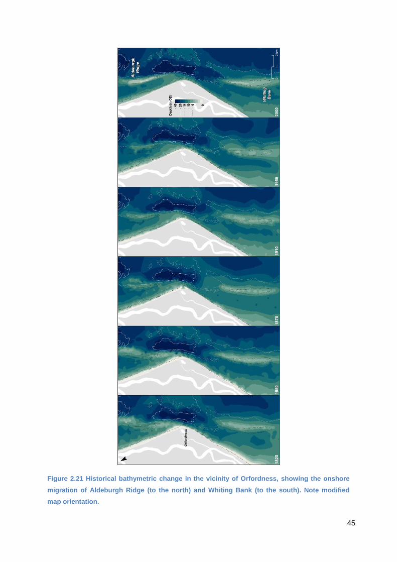
45
Figure 2.21 Historical bathymetric change in the vicinity of Orfordness, showing the onshore
migration of Aldeburgh Ridge (to the north) and Whiting Bank (to the south). Note modified
map orientation.
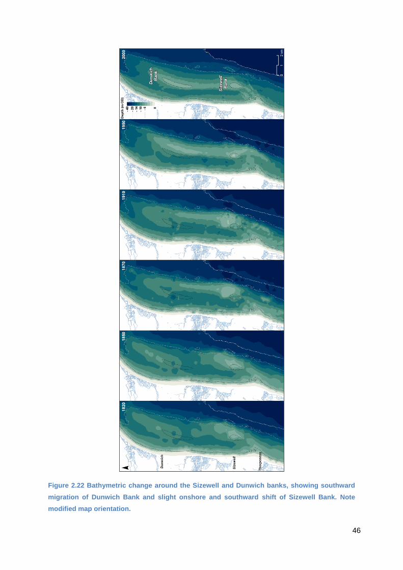
46
Figure 2.22 Bathymetric change around the Sizewell and Dunwich banks, showing southward
migration of Dunwich Bank and slight onshore and southward shift of Sizewell Bank. Note
modified map orientation.
47
The Lowestoft shoreface is rather more complicated morphologically (as shown in the most
recent bathymetry in Figure 2.23), and the interaction between Newcome Sand and Barnard
is not entirely clear. Higher resolution analysis could possibly unravel these complexities, but
early historical surveys for this region contain insufficient data. The historical analysis shows
that the consequence of the northward migration of Barnard (linked directly to the northward
migration of Benacre Ness) was a complex merger with Newcome Sand. In the early 19th
century, Barnard was considerably south of Lowestoft, and Newcome Sand was connected
to the Lowestoft Ness. In this configuration, the seabed in this bay was deepest immediately
offshore from Pakefield.
Over the following decades, Barnard moved northward into the bay, and Newcome Sand
shifted slightly southward, leading to the connection and morphological integration of the two
systems. Small channels have persisted between or around the banks, but these are
spatially and temporally variable. Shoreline changes here are either large-scale accretion
(associated with Benacre Ness) or variable, with clear episodes of small-scale retreat and
advance. These latter shoreline movements likely reflect the complicated movement of small
bank and channel features. There is no evidence to suggest that the dynamics of either the
Benacre Ness foreland or the Barnard offshore bank are driving the combined northward
migration, but rather that they are both responding to a common forcing factor.

48
Figure 2.23 Historical bathymetric change around Barnard and Newcome Sand. The temporal
and spatial resolution of the data cannot resolve the finer aspects of morphological change at
Newcome, but do show that Barnard has moved in connection with the northward migration of
Benacre Ness, and is now rather more intimately connected to Newcome than a century ago.

49
3. Sediment budget
3.1 Data and approach
Cross-shore transects at alongshore intervals of approximately 100 m were derived from the
historical shorelines dataset (Section 2.1) to estimate the alongshore change in sediment
supply resulting from coastal cliff erosion. Topographic profiles extracted from airborne lidar
data have been analysed in the NERC iCOASST project (Nicholls et al., 2012) to assess the
morphology of Suffolk coastal cliffs and the nature of the contemporary sediment system. In
combination, these results were used to calculate: i) estimates of volumes associated with
historical cliff retreat, ii) the total area of the Suffolk coastal sediment system for past and
present, and iii) estimated volumes of the entire contemporary sediment system (from cliff
base/backbarrier to shoreline) and change therein over the last 14 years or so. These
analyses extend the cliff retreat and sediment budget work of others (e.g. Carr, 1981;
McCave, 1987; Brooks and Spencer, 2010) through a higher resolution, region-wide
assessment of the changing sediment system and sediment sources. Here, we synthesise a
whole-Suffolk coastal analysis, with the inclusion of 1:2500 mapping (where available), mid-
century/2011 aerial photography, and modern shorelines, enabling assessment at a finer
alongshore resolution (100 m interval, in contrast to use of EA topographic profiles that are
typically at 1 km alongshore resolution). Analysis of the sedimentology of the various cliff
units draws from the work of James and Lewis (1996).
3.2 Contemporary sediment system
The Suffolk coastal system comprises a near-continuous intertidal, and in places supratidal,
sedimentary (sand and gravel) unit (Figure 3.1A). The sediment system is defined here as
the inter- and/or supratidal beach-grade sediment (sand and gravel) deposit, delimited at the
seaward extent by the MLW shoreline, and by a boundary (digitised from maps and aerial
photographs) representing the juncture between the beach, beach ridge and/or dune system
and the landward cliff, saltmarsh, seawall and/or embankment. Breaks in the intertidal or
supratidal sediment system occur at estuary mouths (Deben, Alde/Ore and Blyth) and at a
few sites where beach levels have lowered seaward of rock armour and revetment defences
(e.g. East Lane, and some sites at Southwold and Felixstowe Ferry).
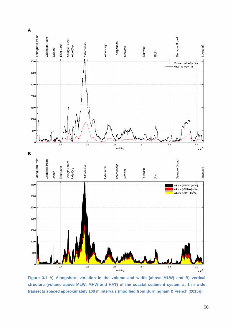
50
A
B
Figure 3.1 A) Alongshore variation in the volume and width (above MLW) and B) vertical
structure (volume above MLW, MHW and HAT) of the coastal sediment system at 1 m wide
transects spaced approximately 100 m intervals [modified from Burningham & French (2015)].
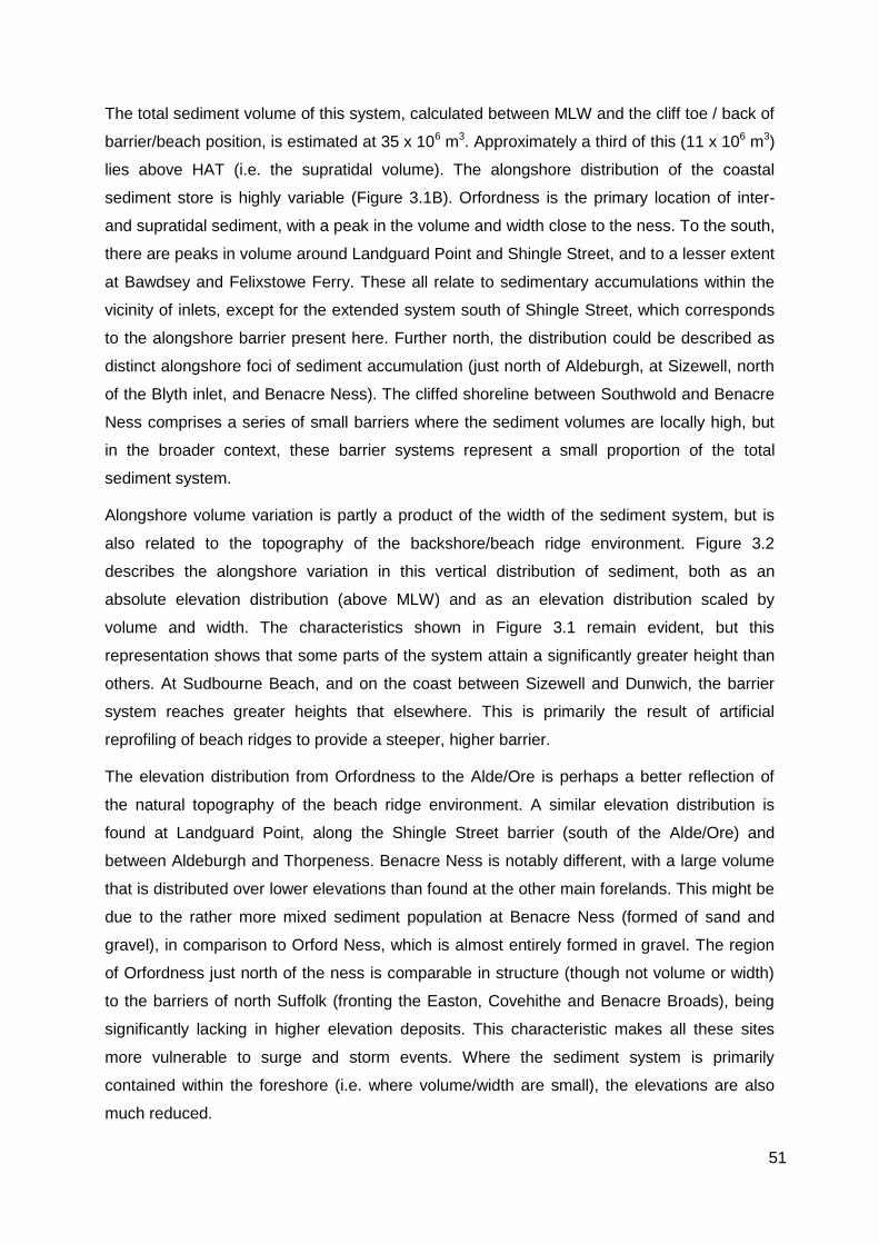
51
The total sediment volume of this system, calculated between MLW and the cliff toe / back of
barrier/beach position, is estimated at 35 x 106 m3. Approximately a third of this (11 x 106 m3)
lies above HAT (i.e. the supratidal volume). The alongshore distribution of the coastal
sediment store is highly variable (Figure 3.1B). Orfordness is the primary location of inter-
and supratidal sediment, with a peak in the volume and width close to the ness. To the south,
there are peaks in volume around Landguard Point and Shingle Street, and to a lesser extent
at Bawdsey and Felixstowe Ferry. These all relate to sedimentary accumulations within the
vicinity of inlets, except for the extended system south of Shingle Street, which corresponds
to the alongshore barrier present here. Further north, the distribution could be described as
distinct alongshore foci of sediment accumulation (just north of Aldeburgh, at Sizewell, north
of the Blyth inlet, and Benacre Ness). The cliffed shoreline between Southwold and Benacre
Ness comprises a series of small barriers where the sediment volumes are locally high, but
in the broader context, these barrier systems represent a small proportion of the total
sediment system.
Alongshore volume variation is partly a product of the width of the sediment system, but is
also related to the topography of the backshore/beach ridge environment. Figure 3.2
describes the alongshore variation in this vertical distribution of sediment, both as an
absolute elevation distribution (above MLW) and as an elevation distribution scaled by
volume and width. The characteristics shown in Figure 3.1 remain evident, but this
representation shows that some parts of the system attain a significantly greater height than
others. At Sudbourne Beach, and on the coast between Sizewell and Dunwich, the barrier
system reaches greater heights that elsewhere. This is primarily the result of artificial
reprofiling of beach ridges to provide a steeper, higher barrier.
The elevation distribution from Orfordness to the Alde/Ore is perhaps a better reflection of
the natural topography of the beach ridge environment. A similar elevation distribution is
found at Landguard Point, along the Shingle Street barrier (south of the Alde/Ore) and
between Aldeburgh and Thorpeness. Benacre Ness is notably different, with a large volume
that is distributed over lower elevations than found at the other main forelands. This might be
due to the rather more mixed sediment population at Benacre Ness (formed of sand and
gravel), in comparison to Orford Ness, which is almost entirely formed in gravel. The region
of Orfordness just north of the ness is comparable in structure (though not volume or width)
to the barriers of north Suffolk (fronting the Easton, Covehithe and Benacre Broads), being
significantly lacking in higher elevation deposits. This characteristic makes all these sites
more vulnerable to surge and storm events. Where the sediment system is primarily
contained within the foreshore (i.e. where volume/width are small), the elevations are also
much reduced.

52
Figure 3.2 Height distribution (above MLW) of the coastal sediment system, showing the
absolute (relative) distribution, and distributions scaled by sediment system width and volume
[modified from Burningham & French (2015)].

53
3.3 Changes in the coastal sediment system
3.3.1 Recent short-term change
Comparison of the coastal sediment system quantified for 2012/13 with that for 1999 shows
broad similarity over this timescale (Figure 3.3). Analyses are conducted on the supratidal
sediment store only due to the lack of intertidal data for 1999. Also, they do not include
changes associated with erosion into non-coastal sediments (i.e. this does not include
volumetric changes linked to cliff recession).
Significant changes are evident at Benacre Ness (south of Lowestoft) northward migration of
which manifested itself as a negative change on the south side of the foreland and large
scale positive change on the north side. Significant change is also evident around
Orfordness. Here, the ness has lost sediment while Sudbourne beach, north of the ness, has
gained sediment. The sediment system along much of the cliff-backed coast has remained
quite stable, with the notable exception of East Lane to Bawdsey, where significant loss of
the non-cliff supratidal sediment unit has been experienced.
The scales of change in volume are small when considered relative to the total volume of the
sediment system and the likely errors in quantifying this volume (Table 3.1). Across the
whole region, the last decade has seen a small net loss in material (4,687 m3), but the
uncertainties (based on an indicative ± 0.1 m Lidar elevation accuracy) are far greater than
this. Within the region, data for Landguard to Deben and Blyth to Lowestoft imply a decrease
in sediment volume, with a small increase in between the Deben and the Alde/Ore, and an
increase between the Alde/Ore and the Blyth. As before, it must be emphasized that the
magnitude of these net changes is much smaller than the uncertainties in the data.
Directions of change in volume largely match those in width. There is thus little evidence for
vertical accretion on existing beach ridges. This is, to some extent, corroborated by
comparison of the overall elevation distribution over this time scale (Figure 3.4). There are
subtle changes in the vertical structure, with the most recent data exhibiting a slightly more
even distribution of elevations, but there is little to differentiate these structural signatures.

54
Figure 3.3 Change in volume and width of the supratidal (>HAT) sediment system from 1999 to
2012/13 [modified from Burningham & French (2015)]. Grey bands denote locations where the
sediment system is backed by high ground; green shows the presence of sea defences
(seawalls, embankments).
Table 3.1 Change in the area and volume of the Suffolk coastal sediment system in recent
years, relative to various tidal datum levels [modified from Burningham & French (2015)].
Volume (to HAT) [m3]
Suffolk Landguard to
Deben
(~10km)
Deben to
Alde/Ore
(~10km)
Alde/Ore to
Blyth
(~37km)
Blyth to
Lowestoft
(~20km)
1999 11,678,589 289,479 789,111 8,945,204 1,654,794
2012/13 11,673,902 279,441 797,318 8,948,118 1,649,026
Change -4,687 -10,038 1,304 44,709 -63,780
Uncertainty ±715,620 ±31,140 ±54,990 ±505,150 ±124,330

55
Figure 3.4 Comparison of the coastal sediment system elevation frequency distributions
landward of HAT (between 1999 and 2012/13) for A) the whole Suffolk coastline, B) Lowestoft to
the Blyth, C) Blyth to Alde/Ore, D) Alde/Ore to Deben and E) Deben to Landguard Point
[modified from Burningham & French (2015)].
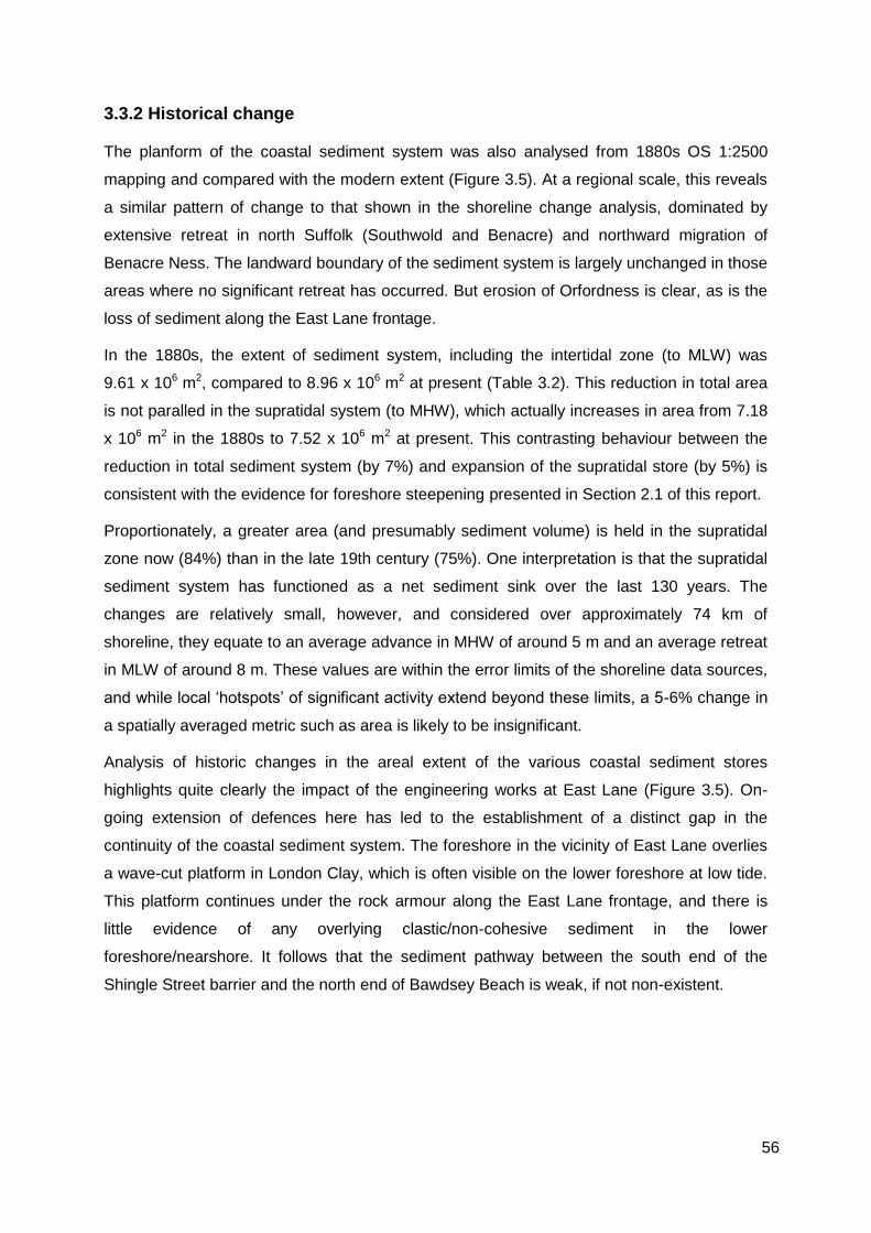
56
3.3.2 Historical change
The planform of the coastal sediment system was also analysed from 1880s OS 1:2500
mapping and compared with the modern extent (Figure 3.5). At a regional scale, this reveals
a similar pattern of change to that shown in the shoreline change analysis, dominated by
extensive retreat in north Suffolk (Southwold and Benacre) and northward migration of
Benacre Ness. The landward boundary of the sediment system is largely unchanged in those
areas where no significant retreat has occurred. But erosion of Orfordness is clear, as is the
loss of sediment along the East Lane frontage.
In the 1880s, the extent of sediment system, including the intertidal zone (to MLW) was
9.61 x 10⁶ m2, compared to 8.96 x 10⁶ m2 at present (Table 3.2). This reduction in total area
is not paralled in the supratidal system (to MHW), which actually increases in area from 7.18
x 106 m2 in the 1880s to 7.52 x 10⁶ m2 at present. This contrasting behaviour between the
reduction in total sediment system (by 7%) and expansion of the supratidal store (by 5%) is
consistent with the evidence for foreshore steepening presented in Section 2.1 of this report.
Proportionately, a greater area (and presumably sediment volume) is held in the supratidal
zone now (84%) than in the late 19th century (75%). One interpretation is that the supratidal
sediment system has functioned as a net sediment sink over the last 130 years. The
changes are relatively small, however, and considered over approximately 74 km of
shoreline, they equate to an average advance in MHW of around 5 m and an average retreat
in MLW of around 8 m. These values are within the error limits of the shoreline data sources,
and while local ‘hotspots’ of significant activity extend beyond these limits, a 5-6% change in
a spatially averaged metric such as area is likely to be insignificant.
Analysis of historic changes in the areal extent of the various coastal sediment stores
highlights quite clearly the impact of the engineering works at East Lane (Figure 3.5). On-
going extension of defences here has led to the establishment of a distinct gap in the
continuity of the coastal sediment system. The foreshore in the vicinity of East Lane overlies
a wave-cut platform in London Clay, which is often visible on the lower foreshore at low tide.
This platform continues under the rock armour along the East Lane frontage, and there is
little evidence of any overlying clastic/non-cohesive sediment in the lower
foreshore/nearshore. It follows that the sediment pathway between the south end of the
Shingle Street barrier and the north end of Bawdsey Beach is weak, if not non-existent.
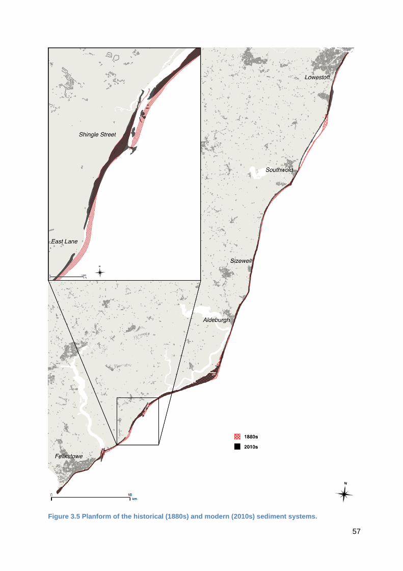
57
Figure 3.5 Planform of the historical (1880s) and modern (2010s) sediment systems.

58
Although the rationale for maintaining and extending defences here is multifaceted (e.g.
cultural heritage, conservation, farming, economic), there appears to be a consensus that
retaining a hard structure at East Lane is essential to preserve the configuration of the bay
since it acts as a downdrift anchor for longshore sediment transport within Hollesley Bay
(Royal Haskoning, 2010). The recent history here is one of gradual barrier recession in the
south concurrent with shoreline advance closer to Shingle Street. This can be explained by a
southward movement of sediment, which would effectively remove sediment from the barrier
to the north of East Lane assuming supply to the north ceased. But the contemporary
configuration of the Shingle Street shoreline implies northward sediment transport in the
vicinity of the Alde/Ore inlet (Figure 3.5 inset). The rotation here might reflect a weakening
and/or reversal of the southward sediment flux.
Table 3.2 Historical change in the area of the Suffolk coastal sediment system [modified from
Burningham & French (2015)].
Area (to MLW) [m2]
Suffolk Landguard to Deben (~10km)
Deben to Alde/ Ore (~10km)
Alde/Ore to Blyth (~36km)
Blyth to Lowestoft (~19km)
1880s 9,605,496 597,978 1,278,898 6,107,258 1,621,362
2012/13 8,963,092 602,129 928,126 5,584,186 1,848,651
Change -642,404
(-7%) 4,151 (+1%)
-350,772 (-27%)
-523,072 (-9%)
227,289 (+14%)
Area (to MHW) [m2]
Suffolk Landguard to Deben (~10km)
Deben to Alde/ Ore (~10km)
Alde/Ore to Blyth (~36km)
Blyth to Lowestoft (~19km)
1880s 7,181,022 266,372 506,876 5,204,375 1,203,399
2012/13 7,521,251 386,178 595,366 5,055,076 1,484,631
Change 340,229 (+5%)
119,806 (+45%)
88,490 (+17%)
-149,299 (-3%)
281,232 (+23%)
3.4 Sediment sources
The sands and gravels that comprise most of the Suffolk coastal sediment system are
primarily sourced from past and present cliff erosion. The rate of sand and gravel supply will
have a direct impact on beach volumes and sediment delivery to the wider sediment system.
The Suffolk cliffs comprise sand, gravel and mud but are dominated by sand (James and

59
Lewis, 1996). On average, sediment supplied from the cliffs north of Southwold comprises
81% sand, 16% mud and 3% gravel. The mid-Suffolk cliffs (Thorpeness to Dunwich) contain
90% sand, 4% mud and 6% gravel. In contrast, the cliffs at Bawdsey contain 67% sand, 14%
mud and 19% gravel. Several studies have estimated the supply from cliff erosion, using
different methods (e.g. shoreline change analysis or EA topographic profiles) over different
time scales (Cambers, 1975; Carr, 1981; Brooks and Spencer, 2010). Flux estimates are in
the range 5,000 - 50,000 m3 yr-1. These previous studies have alluded to temporal variation
in sediment supply, and highlighted the role of shoreline recession in the release of cliff
sediment. The shoreline change results presented in Section 2.1 also imply significant spatial
and temporal variability in sediment flux.
Cliff sediment release was estimated for historical (1881-2013) and recent (1999-2013) time
periods. For the historical volumes, the end point rate of shoreline change at transects
spaced 100 m along the shoreline were used in combination with contemporary cliff heights
(relative to OD, approximately mean sea level) to generate total volumetric change. The end
point rate ensured that the actual historic change was used rather than a time-averaged
approximation, which should generate more accurate results. Historical hinterland
topography is not available at the resolution used here, and the use of contemporary cliff
heights is a potential weakness in the approach. Modern supply rates were calculated using
topographic transects that extended from the hinterland to the foreshore. Cliff morphology
was assessed for each transect in order to define cliff top (between the face and hinterland),
cliff toe (between the face and beach foreshore/backshore) and the position of the MHW
shoreline. This enabled the calculation of trapezoidal volumes for individual sections of the
cross-shore transect, and the separation of volumetric change in the cliff environment from
that of the backshore (Figure 3.6). Changes in cliff volumes were therefore assessed on the
basis of a cross-shore region of interest that covered the minima to maxima extent of the
recent cliff system, and divided into backshore-cliff (cliff top to MHW) fluxes compared to cliff-
face (cliff top to cliff toe) fluxes.
Results of this analysis are displayed as flux-weighted charts showing the relative grain size
fraction associated with sediment delivery at each cliff location (Table 3.2). These reveal
striking differences in magnitude of sediment flux between the 1881-2013 (Figure 3.7) and
1999-2013 (Figures 3.8 and 3.9) analyses. Comparison of historic (Fgure 3.7) and recent
(Figure 3.8) sediment supply shows that the relative role of the Bawdsey and Dunwich cliffs
has reversed. Recent erosion along the north Bawdsey cliffs is now contributing to a
significant proportion of the overall Suffolk sediment budget. Conversely, the Dunwich-
Minsmere cliffs were historically an important part of the sediment supply system, but the
lack of significant retreat here in recent years has reduced their role in the sediment budget.
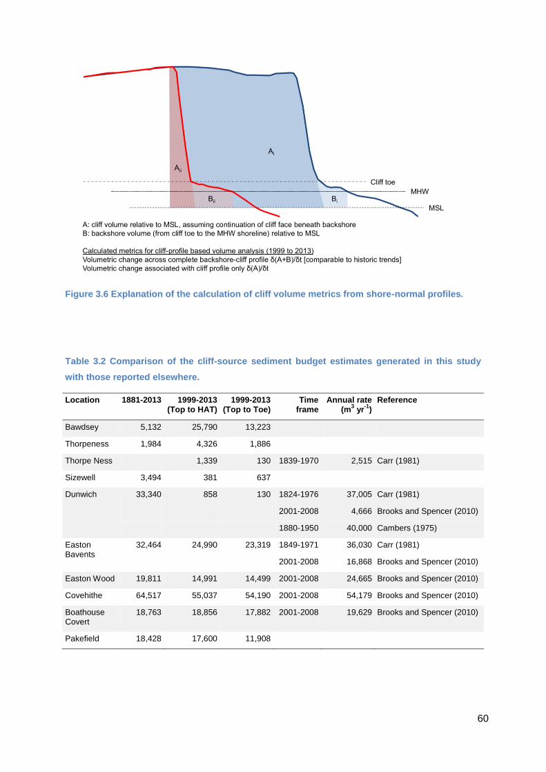
60
Figure 3.6 Explanation of the calculation of cliff volume metrics from shore-normal profiles.
Table 3.2 Comparison of the cliff-source sediment budget estimates generated in this study
with those reported elsewhere.
Location 1881-2013 1999-2013 (Top to HAT)
1999-2013 (Top to Toe)
Time frame
Annual rate (m
3 yr
-1)
Reference
Bawdsey 5,132 25,790 13,223
Thorpeness 1,984 4,326 1,886
Thorpe Ness 1,339 130 1839-1970 2,515 Carr (1981)
Sizewell 3,494 381 637
Dunwich 33,340 858 130 1824-1976 37,005 Carr (1981)
2001-2008 4,666 Brooks and Spencer (2010)
1880-1950 40,000 Cambers (1975)
Easton Bavents
32,464 24,990 23,319 1849-1971 36,030 Carr (1981)
2001-2008 16,868 Brooks and Spencer (2010)
Easton Wood 19,811 14,991 14,499 2001-2008 24,665 Brooks and Spencer (2010)
Covehithe 64,517 55,037 54,190 2001-2008 54,179 Brooks and Spencer (2010)
Boathouse Covert
18,763 18,856 17,882 2001-2008 19,629 Brooks and Spencer (2010)
Pakefield 18,428 17,600 11,908

61
Figure 3.7 Sediment supply associated with coastal cliff recession for the Suffolk shoreline
derived from shoreline change analysis (1881-2013). These results are derived from shoreline
recession rates and cliff heights. See Table 3.2 for a summary.

62
Figure 3.8 Sediment supply associated with coastal cliff recession for the Suffolk shoreline
derived from topographic transect analysis (1999-2013). These results relate to the complete
backshore-cliff profile. See Table 3.2 for a summary.

63
Figure 3.9 Sediment supply associated with coastal cliff recession for the Suffolk shoreline
derived from topographic transect analysis (1999-2013). These results relate to the only the
cliff face region of the shore-normal profile. See Table 3.2 for a summary.

64
The difference between backshore-cliff (Figure 3.8) and cliff-face (Figure 3.9) fluxes is
relatively small, but this varies alongshore. At sites in north Suffolk, the small difference
between these metrics reflects very small backshore volumes that contribute only minimally
to the sediment budget. At sites further south, alongshore variations in the cliff-backshore
profile complicate the estimations. For example, along the south Bawdsey shoreline, a
backshore is evident, but this has been reducing in width with increasing retreat in the cliff
line. Around Thorpeness, an extensive backshore comprising low beach ridges merges with
the shallow sloping cliff profile. Here, the junction between cliff and sedimentary backshore is
less distinct and recessional processes often reflect weathering and breakdown of the broad
cliff profile and re-organisation of backshore/cliff base ridges. To a lesser extent, this is also
the case at Dunwich and Sizewell, where only small scale changes (no significant retreat)
have occurred in recent years, most of which are associated with reworking of the backshore.
The estimates of sediment supply through cliff erosion obtained here are the same order of
magnitude as the few estimates reported by others (Table 3.2). Results from the present
study provide a more detailed breakdown of relative alongshore contribution, and also
recognise the role of sites beyond Dunwich and Easton-Covehithe in the Suffolk-wide
sediment budget. Differences in the selection of alongshore units may account for some of
the discrepancies with the Brooks and Spencer (2010) results. Importantly, the differentiation
of sediment grades shows that currently the erosion at Easton Bavents supplies 31% of cliff-
derived mud, whilst Covehithe supplies 43% of cliff-derived sand, and Bawdsey-East Lane
supplies 35% of the cliff-derived gravel to the Suffolk sediment budget overall. The extensive
erosion of the north Suffolk cliffs in total contributes 95% of cliff-derived mud, 89% of cliff-
derived sand and 62% of cliff-derived gravel to the system.
Shoreline retreat rates tend to overestimate the sediment volumes contributed from cliff
erosion alone as they assume that a retreat in the shoreline equates to retreat of the cliff face.
The relationship between cliff and shoreline retreat is not so clear-cut, and although weak
correlations exist, the relationship is ill defined. Figure 3.10 presents the correlations
between shoreline (MHW) retreat and cliff top, face and base recession. The correlation
coefficients are mostly weak (0.08 < R2 < 0.18), but are improved (0.46 < R2 < 0.54) when
only the most rapidly changing cliffs (cliff position change > 0.5 myr-1) are included in the
analysis. Change in the position of MHW does not seem to be a good predictor of cliff retreat.
But a strong relationship between cliff top and cliff toe recession does exist (R2 = 0.97).
These results show that cliffs are generally undergoing parallel retreat (cliff top and cliff toe
recession at comparable rates), but that the backshore complicates the inter-relationship
between shoreline and cliff retreat.

65
Figure 3.10 Correlation between shoreline (MHW) and cliff (top, face and toe) retreat.
3.5 Geomorphological evidence of sediment transport
The broad-scale geomorphology of the Suffolk coast implies a strong southerly drift of
material, and this has been presented as the dominant transport direction for over a century
now (e.g. Redman, 1864; Steers, 1927; Onyett and Simmonds, 1983; Motyka and Beven,
1987). But the large fluxes of sediment transport that are alluded to in 19th century writing,
including problems of sediment accumulations within the region of Landguard Point (Redman,
1864) are clearly not experienced in the contemporary system. Orford Spit is a good example
of a system where the large-scale geomorphology presents a strong signature of southerly

66
sediment transport, but where scales and directions of change have changed considerably
over the last few centuries. Orfordness itself is the product of large-scale southerly sediment
transport, and Orford Spit that extends southwest of this, diverting the channel of the
Alde/Ore estuary several km south, implies significant southerly transport. The position of
North Weir Point, which marks the southerly extent of Orford Spit, was collated from previous
studies (e.g. Carr, 1972; Carr, 1985) supplemented with satellite/aerial evidence from the
20th century to reconstruct the long-term history of spit dynamics (Figure 3.11). This provides
evidence that the period 1500 to 1800 was characterised by significant elongation of the spit,
with the construction phase clearly driven by considerable alongshore sediment transport.
The most southerly extent recorded was in the early 1800s, since when the spit has
shortened by approximately 2 km. The spit continued to exhibit dynamic behaviour through
the 19th century and early 20th century, but the net product of these dynamics was largely
recessional. Since the mid 20th century, the spit has continued to recede, and is currently
around 1 km shorter than in 1900. The scales of change have reduced considerably,
presumably due to the reduction in alongshore sediment flux.
Evidence from contemporary sources (aerial photography and lidar data) shows that
sediment transport directions on the Suffolk coast are spatially and temporally varied (Table
3.3). The available resources present a random sample of time snapshots between 2000 and
2013 within which the presence of accumulations on the south or north side of alongshore
structures (i.e. groynes) was used to signify evidence of northward or southward sediment
transport (respectively). Earlier maps and charts provided insufficient evidence (and hence
likely time-averaged morphology).
Across this sample, 45% of all results showed northward sediment transport and 35%
showed southward transport: 20% showed no particular bias. Three time periods showed
inconsistent trends, meaning that some parts of the coastline showed northward transport
and other stretches showed southward transport. The wave climate at Southwold, Sizewell
and West Gabbard was analysed to describe the conditions in the 2 days prior to each aerial
survey (Table 3.3). In 83% of the cases, the geomorphic evidenced matched the wave
conditions, that is northward transport was associated with southerly waves and southward
transport with northeasterlies. This shows that local sediment transport is responsive to
changes in offshore wave climate, and that the local morphology is a good indicator of this.
Furthermore, it implies that southerly waves and northward transport are perhaps more
common or important than has hitherto been acknowledged.

67
Figure 3.11 Historical changes in the southerly extension of Orford Spit [modified from
Burningham (2015)].
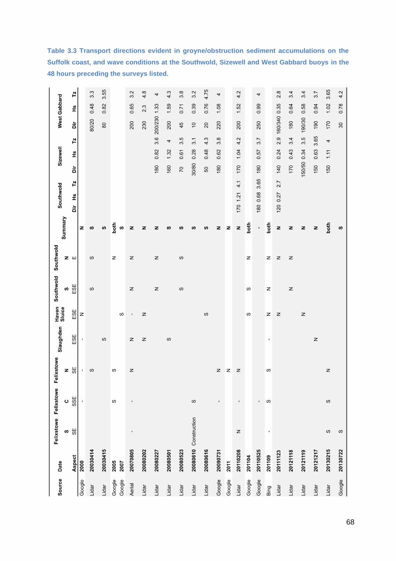
68
Table 3.3 Transport directions evident in groyne/obstruction sediment accumulations on the
Suffolk coast, and wave conditions at the Southwold, Sizewell and West Gabbard buoys in the
48 hours preceding the surveys listed.
69
4. Wave modelling
4.1 Coastal wave climate
The coastal wave climate in Suffolk is relatively well documented in the form of a growing
archive of records from directional wave buoys The Environment Agency operate Directional
Waverider Buoys (DWBs; Environment Agency, 2013) located offshore of Felixstowe,
Sizewell and Southwold. Additional buoys, operated as part of the WaveNet programme are
located at West Gabbard about 30 km offshore of East Lane, and South Knock, to the south
of the immediate study area. Data from these buoys has recently been analysed as part of
the NERC-funded iCOASST project (Nicholls et al., 2012) since Suffolk is one of two test
sites for new estuary and coastal morphological change models being developed.
The longest of the records is that for West Gabbard (commencing 2002), with Sizewell
recording since 2008, Southwold and South Knock 2010, and Felixstowe 2012. Summary
wave climate roses are presented in Figure 4.1 (for buoy locations, refer to Figure 4.4).
These show wave directions (binned at 10° intervals) and frequencies, together with
significant wave height, Hs (colour coded, in metres). The three coastal locations show a
dominant northeasterly mode at Southwold that shifts progressively towards the east by
Felixstowe. A second southerly modal direction is very evident at Southwold and Sizewell,
although this degenerates and shifts towards the southwest at Felixstowe. The two more
offshore locations experience slightly larger waves (50th and 99th percentile Hs around 0.8
and 3.0 m at both sites), with West Gabbard showing strong northeasterly and south-
southeasterly modes and South Knock being characterised by a similarly strong northeast
mode but a broader spectrum of southwesterly directions.
This bimodal wave climate, where over 85% of waves recorded offshore originate from either
the northeast or the south clearly has implications for coastal sediment transport. With the
modifying influence of the various bank systems, it contributes to a more complex pattern of
longshore transport than the predominantly north to south drift system that is commonly
envisaged (SNSSTS, 2002). Numerical modelling of longshore variation in wave power and
sediment transport immediately south of Lowestoft (Coughlan et al., 2007) and in the vicinity
of Benacre Ness (Burningham and French, 2014) has shown the importance of the offshore
sand banks in the attenuation of northeasterly waves (Figure 4.2) and the resulting
significance of southerly waves in generating localised drift reversals. To date, however, high
spatial resolution wave and sediment transport modelling has been restricted to a few
specific locations, and regional assessments (e.g. SNSSTS, 2002) have been undertaken at
much lower resolution.
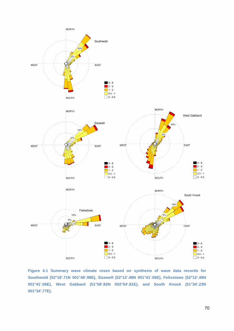
70
Figure 4.1 Summary wave climate roses based on synthesis of wave data records for
Southwold (52°18'.71N 001°46'.98E), Sizewell (52°12'.48N 001°41'.06E), Felixstowe (52°12'.48N
001°41'.06E), West Gabbard (51°58'.82N 002°04'.81E), and South Knock (51°34'.23N
001°34'.77E).

71
Figure 4.2 Numerical wave modelling for the region immediately offshore of Kessingland and
Benacre Ness, showing importance of Newcome and Barnard Sands in locally reduced wave
energy along the beach and (inset table) increasing the relative importance of southerly waves
south of Benacre (reproduced from Burningham and French, 2014).
72
4.2 Numerical wave and longshore transport modelling
4.2.1 SWAN wave model
SWAN (Simulating WAves Nearshore) wave model (Holthuisjen et al. 1993; Booij et al.
1999) is a third-generation numerical model code that incorporates state-of-the-art
formulations for the processes of wave generation, dissipation and wave-wave interactions.
SWAN is fully spectral (in all directions and frequencies) and is ideally suited to computing
the evolution of wind waves in coastal regions. The model code is fully open source and can
be freely obtained from the developers at: http://www.swan.tudelft.nl. In the present
application, SWAN is forced with a series of prescribed deep water wave fields imposed
along an offshore boundary and used to calculate shoaling and refraction over a high
resolution bathymetric grid. Information on nearshore wave conditions is then extracted along
a computational shoreline delimited by the nearshore 2 m depth contour.
4.2.2 Prediction of potential longshore sediment transport
Predictive modelling of wave-driven longshore sediment transport is generally founded on
the premise that the transport rate is proportional to the longshore component of the wave
power, P, per unit length of beach. One of the most widely used formulations is the CERC
equation (USACE, 1984), which predicts sediment transport rate, Qt,vol (volume per unit time)
as
Qt,vol =rK g /gbr
16 rs - r( ) 1- p( )Hsbr
2.5 sin 2q( ) [1]
where K is an empirical calibration coefficient, rs and r are the densities of the sediment
grains and water respectively, g is the acceleration due to gravity, p is a porosity factor
(typically 0.4 for sand), Hsbr is the significant wave height at breaking, q is the wave angle
at the breaker line, and gbr is the breaking coefficient (Hsbr / hbr≈ 0.8, where hbr is the water
depth at wave breaking). The CERC formulation contains no explicit representation of
sediment grain size and its initial calibration was restricted to sand beaches. Various studies
have attempted to extend its applicability to gravel beaches through the use of a lower value
of K. One such study by Nichols and Wright (1991), on two gravel-dominated beaches in
southern England (Hengistbury and Hurst Castle Spit), found that values of K between 1%
and 15% of the widely used value for sand provided the best fit with observed transport rate.

73
A more complete formulation is that by Kamphuis (1991), which includes the effect of both
grain size and beach slope. In this scheme, the mass transport rate, Qt,mass (mass per unit
time) as
Qt,mass = 2.27rs / rs - r( )Tp0.5 d50( )
-0.25(tanb)0.75Hsbr
2(sin(2q))0.6 [2]
where Tp is the peak wave period, d50 is the median grain size and tanb is the beach slope.
This equation has again been primarily calibrated against and performs best for sandy
beaches, and tends to over-predict for gravel (Kamphuis, 1991; Tomasicchio et al., 2013;
van Rijn, 2014). Following van Rijn (2014), volume and mass transport rates can be inter-
converted using the relation
Qt,mass = 1- p( )rsQt,vol [3]
where the porosity value, p, takes a value of 0.4 for sand and 0.45 for gravel. Recently, van
Rijn (2104) has proposed a simple general formulation for longshore transport that is equally
applicable to gravel and sand beaches. This has been evaluated against field and laboratory
observations as well as results from more detailed numerical modelling of sediment transport
processes. In this formulation, Qt,mass is given by
Qt,mass = 0.00018rsg0.5(tanb)0.40 d50( )
-0.6Hsbr( )
3.1(sin(2q) [4]
In this scheme, the rate of longshore sediment transport increases very strongly with
increasing wave height and decreases more rapidly as grain size is increased. As van Rijn
(2014) notes, the transport rate of 20 mm shingle is a factor of 10 lower than that for 0.2 mm
sand. There is also some dependence on beach steepness. In the context of the preceding
analysis of beach steepening along the Suffolk coast (Section 2.1.5), it is interesting to note
that steeper beaches, by virtue of the larger wave heights at the breaker line, tend to favour
higher rates of wave-driven longshore transport. It must be emphasised, however, that the
datasets used to calibrate all these transport formulations are still quite limited, and studies
that have focused directly on coarse and/or mixed size beaches, are still relatively few in
number.
In the present application to Suffolk, the van Rijn (2014) formulation (equation 4) is used to
predict the potential wave-driven longshore transport of gravel. The beaches of Suffolk
present a particular problem as they are predominantly comprised of a variable mixture of
sand and gravel. Grain size distributions are typically polymodal, with significant variability in
the cross-shore direction as well as within the beach and over time at a particular location
(e.g. Pontee et al., 2004). Alongshore variability also exists although modal gravel sizes
reported by Pontee et al. (2004) for beach profiles within the 15 km stretch of coast between
74
Slaughden and Dunwich are similar enough to discourage any attempt to discern a spatial
trend. Given the absence of any published data to suggest, let alone quantify, any systematic
regional grain size trend, constant d50 values were used in all the simulations performed here.
Three sets of simulations were performed, one with a value of d50 = 0.4 mm to represent a
sand mode, one with d50 = 6 mm to represent the fine gravel mode and another with d50 = 25
mm to represent the coarse gravel mode.
Beach slope is known to exhibit more obvious geographical variation (see Section 2.1.5) and
has been quantified at 100 m intervals as part of the analysis of the shore-normal profiles.
Accordingly, the longshore transport simulations include a spatially variable tanb term.
4.2.3 Model domain and bathymetry
Bathymetry exerts a strong influence on hydrodynamics and sediment transport in shallow
coastal and estuarine environments (Cea and French, 2012), and is a critical factor
determining the pattern of wave shoaling and refraction and therefore sediment transport at
the coast (Bender and Dean, 2003). Preparation of an appropriate bathymetric grid for the
wave model domain thus needs to be undertaken with care. Various studies have
demonstrated the sensitivity of coastal wave model results to the resolution of the
bathymetric grid, especially in areas characterised by complex topography such as linear
ridges and banks. A recent assessment by Bunny (2011), for example, demonstrated a
significant improvement in the ability of a SWAN model to reproduce observed wave
generation and propagation off the North Norfolk coast using a 1 km bathymetric grid
compared to the 12 km grid WAVEWATCH-III model used operationally by the Met Office.
Whilst this is an extreme example, it is clear that the spatial resolution of the bathymetry will
exert a major control on the ability of any model to resolve the propagation and dissipation of
wave energy along the Suffolk coast, with its complex bank systems.
Various composite bathymetric datasets exist, but these were considered to be of insufficient
quality for the present purpose or else were not readily available to this study. The SeaZone
Hydrospatial gridded bathymetric product, for example, has multiple artefacts and does not
resolve of the offshore banks and estuary approaches well enough for wave modelling
applications. Accordingly, use was made of raw UK Hydrographic Office (UKHO) survey
datasets recently made available under an Open Government licence via the INSPIRE portal.
All available UKHO data within a region large enough to take the boundaries of a wave
model well away from the Suffolk shoreline of interest were acquired and screened for extent
and date of survey. A composite dataset was assembled based on two criteria: use of the
most recent survey where multiple surveys exist for the same area, and the minimisation of

75
overlap between surveys to avoid conflict between datasets in areas where change has been
significant over the interval between survey dates. The 64 UKHO surveys used are listed in
Appendix 1 (Table 8.3).
Figure 4.3 summarises the survey coverage within a region of interest extending 105 km
south to north and 60 km west to east. This extends as far North as the readily accessible
UKHO survey datasets permit, which is far enough to allow imposition of northeasterly wave
forcing along the eastern boundary when required, whilst minimising the risk of edge effects
impinging on the coast south of Lowestoft. The composite merged dataset comprised
approximately 7 million data points, with the most recent surveys of the approaches to
Lowestoft being especially dense and accounting for most of these. The earliest 1982
surveys are much sparser. A few voids in the UKHO coverage had to be filled using manually
digitised bathymetry from published charts. Throughout the region of interest, the data
density of the composite dataset is sufficient to allow gridding to a 50 m interval. This
provides good resolution of the principal morphological features offshore and is considered to
be a practical computational limit at this time
The raw UKHO datasets contain latitude/longitude positions relative to the WGS 1984
ellipsoid and depths relative to local chart datum. For consistency with the analyses of
shoreline change, positions were projected to British National Grid using the WGS84
(ETRF89) to OSGB36 7-parameter Helmert (‘Petroleum’ transformation) and depths were
referenced to Ordnance Datum (OD), which approximates to mean sea level. This was
achieved using an empirical correction derived from geographical variation in tidal levels
between Lowestoft and Walton-on-the-Naze. Data were then gridded at a 50 m interval,
resulting in the bathymetry shown in Figure 4.4. As with all composite datasets, the
bathymetric grid is a compromise, not least in terms of the fairly wide range of survey dates
involved. These ranged from 1982 to 2006 and Figure 4.5 summarises the way that the
patchwork of different survey dates has been stitched together.

76
Figure 4.3 Visualisation of the extent of each of the UKHO datasets (approximated as convex
hulls; actual survey extents are less regular) used in the composite bathymetric grid.

77
Figure 4.4 Gridded 50 m interval bathymetry derived from UKHO survey data, as used in SWAN
model runs. Rectangle shows extent of smaller region used to extract output from SWAN.
Depths given in metres relative to OD (mean sea level).

78
Figure 4.5 Age distribution of composite gridded bathymetry, based on published survey date.

79
4.2.4 Model setup and forcing scenarios
All simulations were performed using SWAN Cycle III version 41.01. Given that the primary
purpose here is to consider the generalised pattern of wave energy variation and its effect on
potential sediment transport along the coast, a series of steady state (i.e. time-invariant)
simulations were performed using a range of imposed wave conditions imposed along an
offshore boundary of the model domain. Wave generation by wind was not modelled and
SWAN was run in GEN1 mode throughout, generally using default settings. The Madsen et
al. (1988) bottom friction option was used, with a coefficient value of kn = 0.05.
It is clear from the overview of the regional wave climate presented in Section 4.1 that the
key driver of coastal wave conditions is the strongly bi-modal wave direction climate in which
around 85% of waves approach from either a roughly northeasterly or a roughly southerly
direction. Accordingly, coastal wave modelling concentrated on the contrasting alongshore
patterns of wave energy and potential sediment transport that arise under these
characteristic forcing conditions. The objectives are, first, to gain a qualitative insight into drift
directions associated with specific directions of wave approach; second, to infer the likely
drift direction arising as the net effect of the opposing wave approach directions; and third, to
obtain quantitative estimates of the likely transport rates, especially for the gravel fraction.
As noted in Section 4.1, most of the wave data buoys are too close to shore to provide
offshore boundary conditions for SWAN model runs. The best candidates are the West
Gabbard, which lies close to the eastern margin and South Knock. South Knock lies south of
the model domain and has a more southwesterly directional mode than stations further to the
north. Accordingly, data for West Gabbard provide the basis for the synthetic wave climates
used in all the SWAN model runs reported here.
Wave directions recorded by the wave buoys are referenced to magnetic north, which
required conversion to grid north to align with the gridded bathymetry. This was achieved by
deriving a temporally varying offset between magnetic north and grid north based on the
magnetic declinations calculated using the International Geomagnetic Reference Field
(IGRF) model (www.ngdc.noaa.gov/geomag-web/#declination).
Although initial set-ups progressed through a suite of runs that captured an idealised
representation of the ‘NE’ and ‘S’ directional modes for West Gabbard, further analysis was
undertaken to accommodate the less frequent, but possibly important wave climate from the
southeast. In order to effectively represent the full suite of wave conditions experienced by
the Suffolk coast, the hourly wave records were binned into 10° sectors between 0° (N) and
250° (SW). Wave climate within each 10° bin were summarised based on 10th, 25th, 50th, 75th,
90th, 95th and 99th percentile wave heights and their associated period and spread. This

80
equated to 175 SWAN model runs to represent the combined wave climate of 2009 to 2016
at West Gabbard (Table 4.1).
Table 4.1 Summary of initial SWAN model runs using 10° wave approach sectors at West
Gabbard (imposed on eastern and southern boundary).
Frequency bins
Frequency bins
10 25 50 75 90 95 99
10 25 50 75 90 95 99
Hs
Tp
Dir
ec
tio
n b
in
0-10
0.46 0.69 1.04 1.62 2.15 2.55 3.19
6.5 5.5 5.9 6.2 6.8 7.4 7.9 10-20
0.47 0.67 0.96 1.39 1.91 2.20 2.94
6.6 6.6 6.7 6.8 7.0 7.4 8.2
20-30
0.46 0.65 0.91 1.26 1.71 2.03 2.71
6.1 6.5 6.8 7.0 7.1 7.3 8.1 30-40
0.40 0.56 0.86 1.33 1.95 2.46 3.49
5.6 5.8 6.1 6.3 6.8 7.6 8.6
40-50
0.34 0.49 0.83 1.34 1.90 2.43 3.34
5.2 5.0 5.1 5.6 6.3 7.2 8.2 50-60
0.30 0.45 0.78 1.19 1.65 1.97 2.68
5.1 4.5 4.6 5.1 5.8 6.5 7.1
60-70
0.28 0.41 0.74 1.12 1.57 1.84 2.59
5.1 4.2 4.3 4.9 5.5 6.1 6.9 70-80
0.26 0.36 0.72 1.12 1.53 1.86 2.53
5.3 4.1 4.2 4.8 5.4 6.0 6.6
80-90
0.25 0.36 0.66 1.10 1.63 1.93 2.46
5.0 4.0 4.0 4.6 5.4 6.0 6.7 90-100
0.26 0.36 0.66 1.11 1.68 2.02 2.53
4.5 3.7 4.0 4.5 5.3 6.1 6.6
100-110
0.25 0.35 0.65 1.14 1.70 1.99 2.62
4.4 3.5 3.9 4.5 5.2 6.1 6.9 110-120
0.26 0.35 0.62 1.11 1.63 2.13 2.63
4.2 3.5 4.0 4.5 5.1 6.0 6.6
120-130
0.25 0.36 0.66 1.06 1.75 2.02 2.82
4.3 3.4 3.8 4.4 5.2 5.9 6.6 130-140
0.27 0.40 0.68 1.06 1.62 1.94 2.64
4.0 3.5 3.9 4.4 5.2 5.7 6.5
140-150
0.31 0.45 0.71 1.13 1.54 1.89 2.53
3.8 3.7 4.0 4.5 5.0 5.7 6.3 150-160
0.33 0.48 0.77 1.25 1.85 2.20 3.01
3.8 4.0 4.2 4.8 5.6 6.1 6.9
160-170
0.37 0.53 0.81 1.34 1.91 2.35 3.08
3.9 4.1 4.5 5.1 5.9 6.4 7.1 170-180
0.40 0.58 0.87 1.35 1.93 2.30 3.23
4.0 4.3 4.7 5.4 6.0 6.5 7.4
180-190
0.48 0.72 1.12 1.71 2.35 2.76 3.61
3.9 4.5 5.2 5.9 6.7 7.2 7.8 190-200
0.51 0.74 1.16 1.72 2.26 2.54 3.09
3.8 4.4 5.1 5.7 6.3 6.7 7.1
200-210
0.51 0.72 1.07 1.52 2.02 2.30 2.79
3.6 4.1 4.7 5.2 5.8 6.1 6.5 210-220
0.53 0.77 1.13 1.54 2.02 2.34 2.92
3.5 4.1 4.6 5.1 5.6 6.0 6.5
220-230
0.60 0.85 1.21 1.63 2.03 2.31 2.96
3.5 4.1 4.6 5.2 5.6 5.9 6.5 230-240
0.61 0.90 1.26 1.61 1.93 2.16 2.68
3.4 4.1 4.6 5.0 5.4 5.8 6.1
240-250
0.61 0.88 1.19 1.48 1.77 1.99 2.33
3.4 4.0 4.5 4.8 5.2 5.5 5.8
Dir
Spr
Dir
ec
tio
n b
in
0-10
6.0 6.1 6.0 5.9 5.7 5.9 6.0
44 36 32 27 24 23 21 10-20
15.9 16.1 16.1 16.1 15.5 15.7 15.1
38 33 30 28 25 24 22
20-30
25.1 24.8 24.8 24.8 24.7 24.8 25.2
38 32 29 27 25 24 22 30-40
34.5 34.1 33.8 34.1 34.3 34.6 35.0
42 37 33 29 25 23 21
40-50
44.5 44.1 44.4 44.5 44.3 44.0 43.0
47 43 38 32 27 24 22 50-60
55.1 54.9 55.0 54.8 54.8 54.9 55.0
50 46 40 34 29 26 24
60-70
65.0 64.8 65.0 64.7 64.9 65.0 64.7
50 47 41 35 30 28 24 70-80
75.3 74.8 75.3 74.9 74.8 75.0 75.4
53 48 42 36 30 28 26
80-90
85.0 84.7 84.8 85.1 85.0 86.2 85.3
57 50 42 35 31 28 27 90-100
94.8 95.0 94.8 94.8 95.4 95.4 95.6
59 51 44 35 30 27 23
100-110
104.9 104.6 105.0 105.0 104.5 103.9 105.0
61 55 45 35 30 26 23 110-120
114.5 114.5 114.5 115.1 115.4 115.1 116.1
59 53 48 35 31 27 24
120-130
124.6 124.6 125.2 124.9 125.0 124.7 124.5
60 53 45 37 31 30 27 130-140
134.9 135.0 134.8 135.0 135.3 134.7 136.0
60 50 45 38 32 30 26
140-150
145.2 145.6 145.5 145.4 145.7 145.4 145.8
59 48 43 37 32 28 26 150-160
155.3 155.6 155.6 155.6 155.6 155.6 156.8
57 49 40 33 28 24 24
160-170
165.5 165.9 165.9 165.5 166.0 165.7 165.8
52 44 39 31 26 25 22 170-180
175.3 175.6 175.5 176.1 175.9 176.0 176.0
49 41 35 29 25 24 21
180-190
185.1 185.2 185.4 185.6 186.0 186.0 185.2
45 37 30 25 21 19 18 190-200
194.7 194.8 194.7 194.7 194.5 194.1 193.5
44 36 30 25 23 21 20
200-210
204.5 204.6 204.6 204.6 204.5 204.3 204.2
45 38 33 28 26 26 25 210-220
214.4 214.3 214.5 214.6 214.8 214.3 214.5
45 38 33 29 27 26 26
220-230
224.3 224.4 224.6 224.8 224.8 224.5 224.6
44 37 33 30 28 27 26 230-240
234.9 234.6 235.0 234.6 234.9 234.7 234.1
45 37 34 30 28 28 28
240-250
244.8 244.9 244.6 244.7 244.2 244.4 244.5
45 39 34 32 31 31 29

81
A second set of runs was undertaken to explore the role of interannual variability in the
relative frequency of northeasterly versus southerly wave forcing. Comparison of the 2010
and 2011 wave climates with the combined 2009-2016 wave rose shows that 2010
experienced more northeasterlies and 2011 more southerlies than average (Figure 4.6).
Almost 60% of waves were from the northeast in 2010 (46% 2009-2016 average) in
comparison to almost 55% from the south in 2011 (48% 2009-2016 average). Again, the 10th,
25th, 50th, 75th, 90th, 95th and 99th percentile wave heights and their associated period and
spread were calculated for each 10° directional bin (Table 4.2) and then used to drive an
additional set of longshore transport runs. Finally, the SWAN runs in Table 4.1 were also
recomputed with a variation in water level of +0.75 m. The aim here is to examine the
sensitivity of the longshore sediment direction and potential flux magnitudes to the small
increase in water depth inshore and over the banks that might be expected under current
regional sea-level rise projections. In total, 700 SWAN runs were undertaken.
Steady state SWAN solutions were processed to yield wave conditions at the 2 m water
depth contour located shore-normal from positions at 100 m spacing along the MHW
shoreline. This ensured that wave parameters obtained represented similar nearshore
conditions along the entire coast. A finer model grid, with more detailed nearshore
bathymetry would be required to accurately resolve the breaking point (e.g. Adams et al.,
2011). Along this ‘computational shoreline’, values of Hs, Tp, and q were derived for use in
the estimation of potential longshore sediment transport.
Figure 4.6 Comparison of the 2010 and 2011 wave climates, in the context of the combined
2009-2016 summary wave rose.

82
Table 4.2 Summary of the A) 2010 and B) 2011 wave climates in which relative frequencies of
‘northeasterly’ and ‘southerly’ waves at West Gabbard shift considerably (see Figure 4.6).
These climates are used to force additional longshore sediment transport model runs.
A)
Frequency bins
Frequency bins
2010
10 25 50 75 90 95 99
10 25 50 75 90 95 99
Hs
Tp
Dir
ec
tio
n b
in
0-10
0.43 0.64 1.07 1.82 2.4 2.67 2.98
6.8 5.7 6.3 6.5 7 7.7 7.7 10-20
0.47 0.71 0.99 1.48 2.12 2.42 2.87
6.8 6.7 6.9 6.9 7.5 7.7 8
20-30
0.48 0.66 0.95 1.33 1.86 2.26 2.85
6.3 6.7 6.9 7 7.3 7.6 8.1 30-40
0.4 0.6 1.08 1.58 2.48 3.21 4.06
5.8 6.1 6.2 6.4 7.3 8.5 9.1
40-50
0.34 0.49 1.02 1.47 1.98 2.91 3.92
5.6 5.3 5.2 5.8 6.4 7.8 8.8 50-60
0.29 0.43 0.89 1.22 1.52 1.85 2.79
5.2 4.9 4.8 5.2 5.4 6.4 6.7
60-70
0.27 0.41 0.92 1.16 1.38 1.7 2.25
5.3 4.4 4.4 4.9 5.1 5.8 6.6 70-80
0.25 0.33 0.8 1.16 1.51 1.87 2.31
5.7 4.6 4.4 4.8 5.1 6.2 6.7
80-90
0.25 0.3 0.68 1.12 1.96 2.13 2.33
5.5 4.7 4.1 4.8 5.7 6.6 6.8 90-100
0.26 0.35 0.65 1.19 1.48 1.76 2.42
5.2 4.1 4.1 4.5 5.3 5.4 6
100-110
0.26 0.35 0.74 1.22 1.52 1.81 2.57
4.7 3.4 3.9 4.6 4.9 5.6 7 110-120
0.25 0.31 0.6 1.07 1.38 2.69 3.01
4.5 3.5 3.7 4.4 5 6.7 6.9
120-130
0.23 0.3 0.45 1.01 1.32 1.51 3.11
4.3 3.9 3.4 4.1 4.6 5.2 6.5 130-140
0.25 0.4 0.72 1.05 1.4 1.58 2.56
4.4 3.3 3.9 4.3 4.7 5.4 5.8
140-150
0.26 0.4 0.6 1.05 1.42 1.7 2.42
4.2 3.4 3.9 4.3 4.6 5.3 6.1 150-160
0.29 0.41 0.69 1.25 1.68 2.06 2.62
3.6 3.7 4 4.6 5.5 5.9 6.4
160-170
0.32 0.47 0.68 1.09 1.67 2.13 2.73
3.8 4.2 4.3 4.8 5.4 6.4 6.7 170-180
0.36 0.5 0.75 1.18 1.7 1.95 2.76
4 4.2 4.6 5.1 5.7 6.1 7.3
180-190
0.43 0.57 0.88 1.3 1.93 2.5 3.28
3.9 4.2 4.7 5.3 6.3 7 7.6 190-200
0.44 0.6 0.9 1.3 1.74 2.05 2.59
3.7 4.1 4.5 5.1 5.7 6.1 6.6
200-210
0.45 0.6 0.9 1.31 1.72 1.95 2.39
3.4 3.8 4.4 5 5.4 5.9 6.1 210-220
0.43 0.65 0.98 1.44 1.83 2 2.95
3.3 3.7 4.4 4.9 5.6 5.6 6.7
220-230
0.51 0.72 1.2 1.55 1.86 2.28 3.18
3.2 3.9 4.4 5 5.4 5.7 6.7 230-240
0.56 0.93 1.33 1.58 1.81 1.88 2.83
3.4 4 4.5 4.9 5.1 5.5 5.6
240-250
0.59 0.83 1.21 1.4 1.63 1.71 1.78
3.3 4 4.5 4.8 5 5.3 5.2
Dir
Spr
Dir
ec
tio
n b
in
0-10
6.7 6.4 6.8 6.8 6.7 7.9 6.5
44 35 32 27 24 23 22 10-20
16.4 16.6 16.9 17.1 16.2 16 14.6
38 32 28 26 25 23 22
20-30
25.7 25.4 25.1 25.4 25.1 25 25.7
36 32 28 27 25 23 21 30-40
35 34.5 34.7 34.8 34.7 35.1 35.9
42 35 31 28 24 22 20
40-50
44.4 44.2 44.4 44.3 43.5 44.1 42.8
46 42 36 30 27 25 22 50-60
54.4 54.5 54.5 54.9 54.3 53.4 54.7
50 44 38 34 32 28 27
60-70
64.6 64.2 64.5 64.8 64.1 63.6 63.9
52 47 39 34 32 31 28 70-80
75.8 74.7 74.9 75.1 75 75.2 76.2
52 49 44 35 34 28 26
80-90
86.1 85.3 84.8 85 85.2 86.8 85.3
54 52 43 40 30 26 27 90-100
96.2 95.2 95.8 95.1 96 95.9 96.4
58 50 46 38 36 33 28
100-110
105.3 104.9 106.2 105.5 104.8 108 107.9
62 54 46 34 29 31 24 110-120
115.2 115.5 115.2 115.8 114.8 115.9 118.4
60 54 46 39 28 27 23
120-130
125.7 125.7 125.3 126.5 125.2 124.1 126.1
63 57 48 40 32 28 26 130-140
134.6 135 134.6 133.9 134.3 135 135.6
62 48 46 40 28 28 27
140-150
144.9 145.7 145.6 144.9 143.7 145.7 144.7
59 51 48 37 33 28 26 150-160
155 155.2 155.3 155.1 155.4 154 156.3
57 51 40 34 28 28 24
160-170
165.5 166.4 166 166.1 165.8 166.4 165.3
52 45 39 35 28 26 24 170-180
175.7 175.9 176 176.5 176.9 176 177.7
50 43 37 32 27 24 21
180-190
185.4 185.8 185.7 186.5 185.9 186.7 185.2
47 40 33 30 25 23 19 190-200
195 195.1 195.2 195.7 195.3 195.6 194.5
47 39 33 30 28 26 24
200-210
205.3 205.2 204.8 205 205 205.8 204.6
46 41 36 31 28 28 29 210-220
215.6 214.4 215 215.1 215.1 214.9 216.7
47 40 35 31 30 27 25
220-230
224.8 224.6 224.6 225.2 225.8 223.9 224
45 37 34 33 30 28 24 230-240
234.7 234.1 234.7 234.5 235 233.8 234.3
41 36 33 30 29 28 28
240-250
244 244.9 243.3 244.8 244.4 242.7 242.4
44 39 34 33 33 33 29

83
Table 4.2 cont.
B)
Frequency bins
Frequency bins
2011
10 25 50 75 90 95 99
10 25 50 75 90 95 99
Hs
Tp
Dir
ec
tio
n b
in
0-10
0.43 0.65 1.02 1.35 1.9 2.09 2.36
6.6 5.1 6 5.9 6.7 6.3 7 10-20
0.41 0.65 1 1.43 1.82 1.96 2.26
6.3 6 6.9 7.2 7.3 7.5 7.3
20-30
0.42 0.6 0.9 1.28 1.75 1.95 2.45
6.1 6.2 6.7 7.2 7.3 7.2 7.9 30-40
0.37 0.56 0.84 1.33 1.87 2.07 2.41
5.7 5.9 6.2 6.3 6.7 7.1 7.3
40-50
0.31 0.49 0.81 1.3 1.76 1.96 2.56
5.3 5.4 5.1 5.5 6.1 6.6 7.3 50-60
0.27 0.41 0.77 1.14 1.49 1.61 1.92
5.4 5 4.4 5.1 5.7 5.9 6.3
60-70
0.24 0.31 0.65 1.01 1.39 1.56 1.69
5.6 5 4.2 4.7 5.4 5.6 6 70-80
0.23 0.29 0.6 0.95 1.25 1.38 2.01
5.4 5.2 4.3 4.5 5 5.4 5.8
80-90
0.23 0.3 0.55 1.1 1.35 1.98 2.62
4.8 4.6 4 4.6 5.1 6 7.1 90-100
0.24 0.33 0.61 1.05 1.96 2.16 2.65
4.5 4.2 3.7 4.6 5.5 6.2 6.8
100-110
0.23 0.31 0.48 1.08 1.47 1.98 2.64
4.7 3.7 3.6 4.3 5.1 5.9 6.4 110-120
0.24 0.31 0.45 1.15 1.77 2.12 2.42
4.6 3.5 3.4 4.4 5.2 5.8 6.2
120-130
0.22 0.31 0.46 0.94 1.51 1.96 2.36
4.4 3.8 3.5 4 4.9 5.6 6.1 130-140
0.23 0.32 0.48 1.04 1.68 1.97 2.13
4.1 3.4 3.5 4.4 5.3 5.9 6
140-150
0.25 0.34 0.64 1.17 1.5 1.75 2.04
4 3.3 3.8 4.6 5.2 5.6 5.8 150-160
0.28 0.4 0.69 1.23 1.62 1.8 2.32
3.8 3.8 4.1 4.8 5.3 5.8 6.1
160-170
0.32 0.49 0.74 1.1 1.6 1.85 2.78
3.7 4.2 4.3 4.7 5.5 6 6.8 170-180
0.36 0.54 0.79 1.18 1.63 1.92 2.83
4 4.3 4.5 5.1 5.7 6 6.7
180-190
0.44 0.65 1.04 1.57 2.07 2.38 3.26
3.8 4.5 5 5.7 6.4 7.1 7.5 190-200
0.48 0.71 1.08 1.6 2.06 2.4 2.9
3.8 4.3 4.9 5.5 6.2 6.8 6.9
200-210
0.5 0.74 1.06 1.52 1.94 2.23 2.61
3.6 4.2 4.7 5.2 5.7 6 6.3 210-220
0.53 0.83 1.17 1.56 2.01 2.3 2.6
3.5 4.2 4.6 5.2 5.8 5.9 6.3
220-230
0.58 0.89 1.24 1.63 1.93 2.15 2.41
3.4 4.1 4.5 5.2 5.6 5.8 5.9 230-240
0.67 1.05 1.44 1.74 2.01 2.16 2.46
3.5 4.4 4.9 5.3 5.6 5.8 5.9
240-250
0.67 1.08 1.44 1.75 2.01 2.14 2.33
3.5 4.4 4.8 5.2 5.5 5.6 5.8
Dir
Spr
Dir
ec
tio
n b
in
0-10
5.8 5.8 5.9 6.2 4.9 4.5 4.4
46 37 30 26 25 25 22 10-20
15.6 15.7 15.6 15.5 15 15.5 15.3
41 37 30 27 25 25 24
20-30
25 24.6 24.8 24.5 24.3 24 24.3
39 36 30 28 25 24 23 30-40
34.3 33.9 33.8 34.3 34.2 33.8 33.4
45 39 34 29 24 23 24
40-50
44.6 44 44.5 44.6 44.2 44.2 43.3
51 46 38 31 27 25 24 50-60
55.7 54.3 55.1 54.2 54.3 54.8 54.4
51 51 39 35 30 26 26
60-70
65 64 64.6 64.6 65.1 65.8 64.3
49 53 45 37 36 28 27 70-80
75.4 75.3 75.5 75.2 75.3 73.9 75.5
53 54 48 37 36 32 36
80-90
84.6 84.4 84.7 85.3 85.3 86.6 84.3
58 54 50 37 33 31 26 90-100
94.7 94.6 94.6 95 94.7 96.1 96.1
60 56 46 38 30 23 21
100-110
104.8 104.8 104.9 104.4 104.5 103.3 103.1
59 57 49 38 32 27 23 110-120
114.6 113.5 113.3 114.9 115.3 115.6 115.4
58 56 48 34 32 30 27
120-130
124.6 123.9 124.1 125 125.7 126.5 124.8
64 56 49 42 31 32 25 130-140
134.9 135.6 133.9 135 135.3 133.6 134.4
61 54 49 42 33 30 30
140-150
144.5 144.9 145.5 145.4 145.4 143.9 144.5
61 55 46 39 32 30 29 150-160
155 155.2 155.4 155.1 155.8 155.1 156.4
60 51 43 33 29 26 22
160-170
164.7 166 165.1 165.1 164.7 165.3 166
54 47 40 34 26 24 22 170-180
174.9 175.7 175.6 175.8 176.5 176.1 175.1
51 44 37 30 27 25 19
180-190
184.6 184.9 185.3 185.7 186 186 185.3
46 38 31 26 22 22 19 190-200
194.3 194.6 194.7 194.6 194.7 193.9 194
46 36 31 27 24 23 22
200-210
203.9 204.1 204.6 204.3 204.2 204.9 205.2
45 38 33 29 27 27 25 210-220
214 213.7 214.1 214.2 214.7 213.9 213.6
45 37 31 30 27 27 24
220-230
224.1 224.2 224.5 224.7 225.2 225 225.1
44 37 32 29 28 28 27 230-240
234.3 234.5 234.8 234.6 235.3 234.9 235
43 35 31 29 29 28 31
240-250
244.4 244.4 244.2 244.3 244.6 243.7 244.5
45 34 32 31 30 29 32

84
4.2.5 Wave modelling results
Illustrative output fields for Hs under northeasterly and southerly forcing for the 50th and 99th
percentile deep water Hs values are presented in Figure 4.7. These plots highlight the
opposing nature of the wave direction field, and the high angle of wave approach along much
of the Suffolk coast. Dissipation over the various banks is evident as is the sheltering effect
of the major shoreline protrusions (notably Orford Ness, but also the shoreline offset that has
developed to the north of the Blyth estuary mouth). These effects are especially evident
under northeasterly waves and in the area to the south of Lowestoft. The sheltering effect of
the Newcome and Barnard Sands is evident, and also the shadow zones in the lee of
protrusions subject to high angles of wave approach.
4.2.6 Potential longshore sediment transport
Wave conditions at the shoreline were used to derive two sets of outputs. First, for each 10°
wave direction bin, simulations were performed separately for the 10th, 25th, 50th, 75th, 90th
and 99th percentile wave heights. For each of these runs, the computed potential longshore
sediment transport was weighted by the fractional duration of the specified percentile,
corrected for the fraction of the time that waves approach from the modal wave direction.
Offshore wave directions were not modelled and sediment transport was assumed to be
negligible under these conditions. Second, the net annual sediment transport rate was
computed as the sum of the (generally opposing) transports arising under the north through
to southwest (0° to 250°) forcing waves.
Figures 4.8, 4.9 and 4.10 show the computed potential transport for fine gravel (d50 = 6 mm),
coarse gravel (d50 = 25 mm) and, for comparison, medium sand (d50 = 0.4 mm). Along-coast
variation in potential sediment transport exhibits many features that are consistent with the
analyses presented in the preceding sections of this report. Most obvious, is the expected
north to south transport under northeasterly waves (most evident in Figure 4.8a). This
increases in magnitude south from Lowestoft, with a shadow zone within the bay that is
developing between the mouth of the Blyth and Dunwich, and relatively high potential
transport rates along the coast as far as Orford Ness. Beyond Orford Ness, the southerly
transport is weak and the model results show that it is exceeded in many places by a south
to north transport, driven by waves from the south, most notably between Landguard and
Orford Ness. This is consistent with the morphological evidence discussed in the previous
section, including the alignment of Shingle Street and persistent observations of north-
directed sediment accumulation within groyne bays along the Felixstowe frontage.

85
Figure 4.7 Visualisation of Hs with superimposed direction for wave approaches from 45° (left)
and 185° (right). Top row show 50th
percentile climates (deep water Hs = 0.83 and 1.12 m
respectively (upper left and right)); and 99th
percentile conditions (Hs = 3.34 and 3.61 m
respectively (lower left and right) derived from the 2009-2016 wave record at West Gabbard.
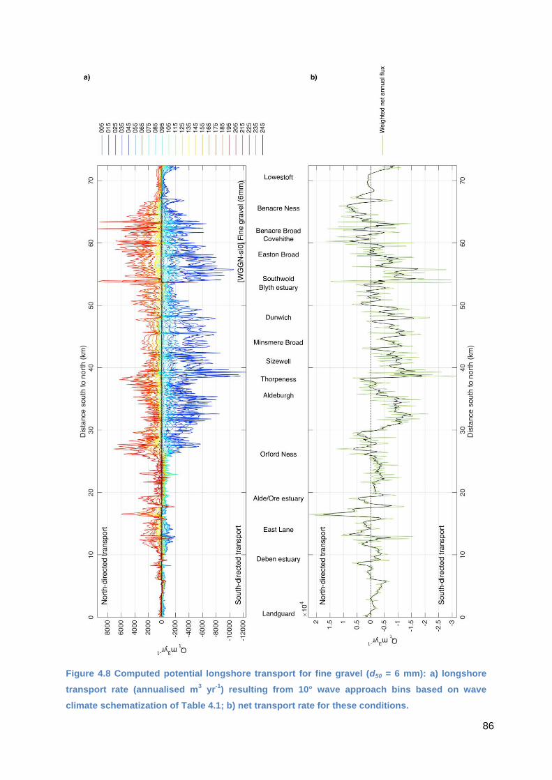
86
Figure 4.8 Computed potential longshore transport for fine gravel (d50 = 6 mm): a) longshore
transport rate (annualised m3 yr
-1) resulting from 10° wave approach bins based on wave
climate schematization of Table 4.1; b) net transport rate for these conditions.

87
Figure 4.9 Computed potential longshore transport for coarse gravel (d50 = 25 mm): a)
longshore transport rate (annualised m3 yr
-1) resulting from 10° wave approach bins based on
wave climate schematization of Table 4.1; b) net transport rate for these conditions.
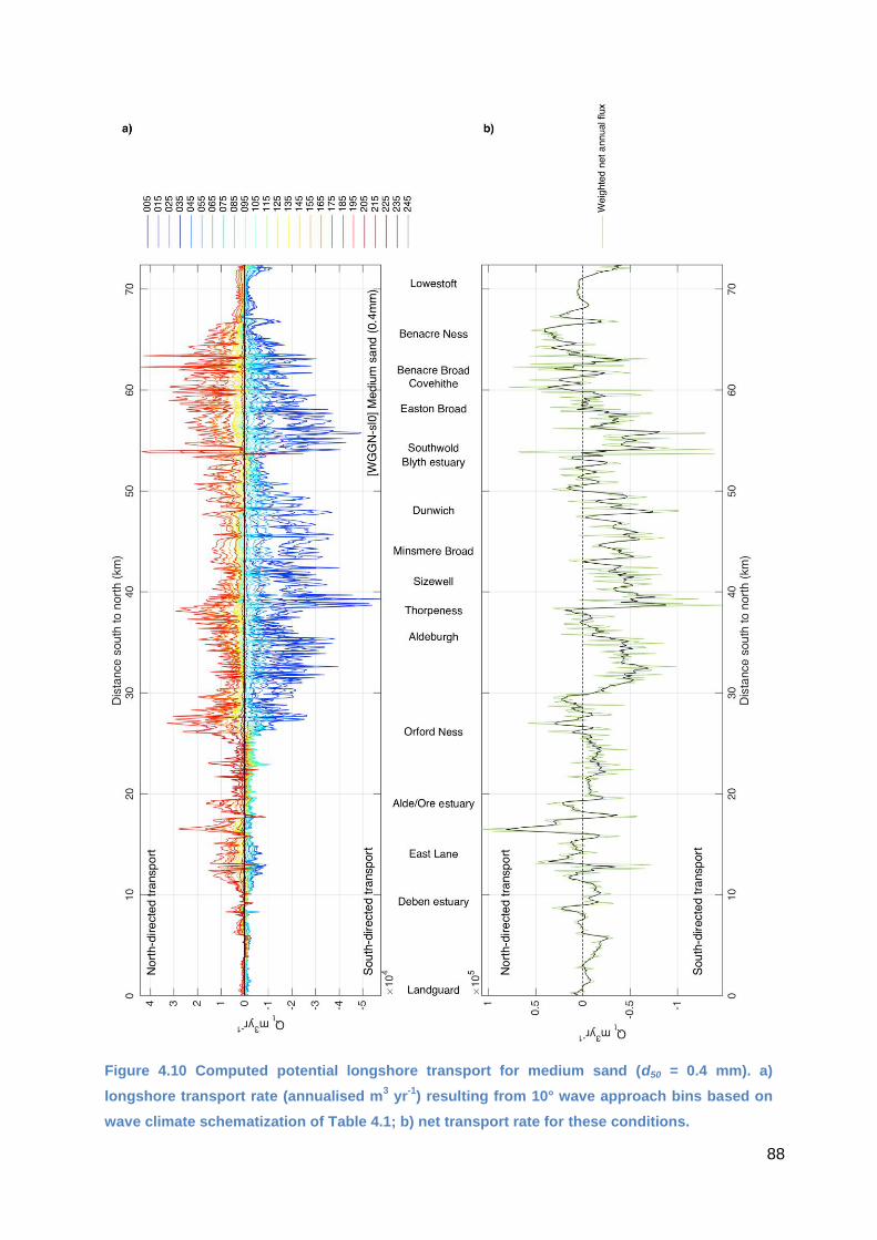
88
Figure 4.10 Computed potential longshore transport for medium sand (d50 = 0.4 mm). a)
longshore transport rate (annualised m3 yr
-1) resulting from 10° wave approach bins based on
wave climate schematization of Table 4.1; b) net transport rate for these conditions.
89
Convergences and divergences in transport are apparent at a number of locations, especially
at Orford Ness, which marks a distinct change in shoreline aspect from southeast to east
facing. This large cuspate foreland might be seen as a natural analogue for a shingle engine
as envisaged in Royal Haskoning DHV (2013). Between the ness and the Alde/Ore entrance
to the south, the net transport is largely southward, but changes to northwards around the
ness before switching back to southwards north of the ness along Sudbourne Beach. This
implies that there is a divergence zone just to the south of the ness and a convergence zone
just to the north. A similar finding emerges in the detailed study of wave-drive transport at
Slaughden reported by HR Wallingford (2016). These shifts appear to be a product of the
change in shoreline orientation in combination with the presence of Aldeburgh Ridge.
As already noted, the effect of the more significant protrusions in creating shadow zones
under high angles of wave approach is particularly evident. This is especially apparent to
both the north and south of Orford Ness and to the south of the Blyth estuary, where the
jetties have created a significant shoreline offset. Also of interest is the fact that Benacre
Ness represents a distinct and extended stretch of south to north littoral drift. It is also just
possible to discern a similar effect at Thorpeness, which stands out as a distinct local
reversal in the middle of a 20-km stretch of south-directed transport. This points to the
influence of this minor ness, and the importance of locally more resistant geology (Coralline
Crag outcropping offshore; Lees, 1980; Carr, 1981).
There is no evidence for any significant differences in this pattern of transport between the
sediment size fractions considered. This is not unexpected given that there is no physics
contained in any of the transport formulations reviewed here that would give rise to
differences in the direction of transport with grain size. Obviously the simulated sand
transport is much larger in magnitude than that for the gravels. In terms of absolute
magnitude, the estimated transport rates generated in the present study are in the same
range as previous work but there is considerable variability and the basis of some of the
earlier studies is difficult to discern.
Tables 4.3 and 4.4 summarise the transport estimates for Suffolk that were drawn together in
the Southern North Sea Sediment Transport Study (SNSSTS, 2002). Our results are in
agreement with previous inferences of relatively weak movement of coarse material along
the coast south of the Deben estuary and it is interesting that only a few studies point to the
existence of a northward pathway here (although our own results do imply opposing and
therefore rather variable north – south transport). At Shingle Street, it is interesting to recall
the observation of Steers (1925) that "South of Shingle Street there is an unbroken line of
shingle in front of the low-lying marshlands and Bawdsey Cliff. This shingle, as elsewhere in
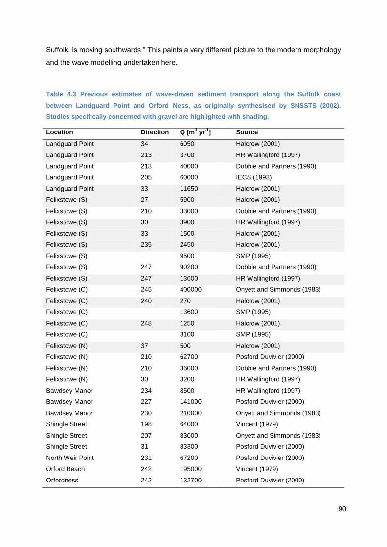
90
Suffolk, is moving southwards.” This paints a very different picture to the modern morphology
and the wave modelling undertaken here.
Table 4.3 Previous estimates of wave-driven sediment transport along the Suffolk coast
between Landguard Point and Orford Ness, as originally synthesised by SNSSTS (2002).
Studies specifically concerned with gravel are highlighted with shading.
Location Direction Q [m3 yr
-1]
Source
Landguard Point 34 6050
Halcrow (2001)
Landguard Point 213 3700
HR Wallingford (1997)
Landguard Point 213 40000
Dobbie and Partners (1990)
Landguard Point 205 60000
IECS (1993)
Landguard Point 33 11650
Halcrow (2001)
Felixstowe (S) 27 5900
Halcrow (2001)
Felixstowe (S) 210 33000
Dobbie and Partners (1990)
Felixstowe (S) 30 3900
HR Wallingford (1997)
Felixstowe (S) 33 1500
Halcrow (2001)
Felixstowe (S) 235 2450
Halcrow (2001)
Felixstowe (S)
9500
SMP (1995)
Felixstowe (S) 247 90200
Dobbie and Partners (1990)
Felixstowe (S) 247 13600
HR Wallingford (1997)
Felixstowe (C) 245 400000
Onyett and Simmonds (1983)
Felixstowe (C) 240 270
Halcrow (2001)
Felixstowe (C)
13600
SMP (1995)
Felixstowe (C) 248 1250
Halcrow (2001)
Felixstowe (C)
3100
SMP (1995)
Felixstowe (N) 37 500
Halcrow (2001)
Felixstowe (N) 210 62700
Posford Duvivier (2000)
Felixstowe (N) 210 36000
Dobbie and Partners (1990)
Felixstowe (N) 30 3200
HR Wallingford (1997)
Bawdsey Manor 234 8500
HR Wallingford (1997)
Bawdsey Manor 227 141000
Posford Duvivier (2000)
Bawdsey Manor 230 210000
Onyett and Simmonds (1983)
Shingle Street 198 64000
Vincent (1979)
Shingle Street 207 83000
Onyett and Simmonds (1983)
Shingle Street 31 83300
Posford Duvivier (2000)
North Weir Point 231 67200
Posford Duvivier (2000)
Orford Beach 242 195000
Vincent (1979)
Orfordness 242 132700
Posford Duvivier (2000)

91
Table 4.4 Previous estimates of wave-driven sediment transport along the Suffolk coast
between Orford Ness and Lowestoft, as originally synthesised by SNSSTS (2002).
Location Direction Q [m3 yr
-1] Source
Orfordness 242 132700
Posford Duvivier (2000)
Aldeburgh 185 80000
Vincent (1979)
Thorpeness 202 55000
Onyett and Simmonds (1983)
Thorpeness 178 300
Halcrow (2001)
Thorpe Ness 178 200000
Onyett and Simmonds (1983)
Sizewell 180 85000
Vincent (1979)
Sizewell 182 3450
Halcrow (2001)
Dunwich Cliffs 0 101000
Vincent (1979)
Dunwich Cliffs 190 130000
Onyett and Simmonds (1983)
Reedland Marshes 198 11000
Halcrow (2001)
Town Salts (Walberswick) 213 148000
Vincent (1979)
The Flats (Walberswick) 224 210000
Onyett and Simmonds (1983)
Southwold 196 200000
Onyett and Simmonds (1983)
Southwold 190 3100
Halcrow (2001)
Covehithe Cliffs 200 18250
Halcrow (2001)
Boathouse Covert 200 105000
Onyett and Simmonds (1983)
Benacre Denes 200 2500
Halcrow (2001)
Benacre Ness 2 28150
Halcrow (2001)
Kessingland Cliffs 2 13000
Onyett and Simmonds (1983)
Pakefield Cliffs 5 41000
Vincent (1979)
Kirkley Cliffs 199 1050
Halcrow (2001)
A few studies have proposed shifts in wave climate as a factor that may underlie changes on
coastal behaviour. Pye and Blott (2006) for example, allude to a possible change in the
frequency and duration of dominant wind and wave directions as a possible factor in
changing coastal wave climate. They suggest a potential weakening of the north to south
littoral drift after about 1925. It is tempting to associate such a shift with the general tendency
towards a less dynamic sediment system since the 19th century. The wave modelling
presented here is consistent with this inasmuch as it reveals a finer and more geographically
varied balance between opposing drift directions than is suggested by, for example, SNSSTS
(2002).
It is not straightforward to generate realistic wave climate scenarios to represent past climate
variability given the short duration of the necessary observational datasets. This applies not
just for wave observations per se but also the meteorological information needed to attempt
hindcasts of historical wave conditions. However, it is instructive to consider the sensitivity of
92
modelled potential transport rates and pathways to plausible shifts in the wave climate. One
such experiment is performed here using the wave climates of 2010 and 2011 as examples
of the interannual variability in the relative frequency of the dominant wave directions.
Although it is not possible to ascertain the extent of longer term changes in directions, the
comparison of 2010 (northeasterly dominated) and 2011 (southerly dominated) net annual
fluxes provides an envelope of variability with which to gauge the impact of directional shifts.
Figure 4.11 shows modelled potential longshore transport using the 2010 and 2011 wave
climates as schematised in Table 4.2 in comparison to the average annual climate 2009-
2016. Given that the spatial variation in potential transport rate is essentially the same for all
sediment size fractions, only the results for the fine gravel fraction (d50 = 6 mm) are plotted.
The changes are small compared to baseline condition, which obviously lies between the two
perturbed cases. Higher energy waves from the northeast in 2010 generate larger fluxes
than the weaker climate of 2011. But there are locations at which the net drift actually
reverses; under the 2010 wave climate, several locations see a switch from north to south-
directed transport whereas for 2011, shifts from south to north-directed transport occur. In
many cases, the drift reversals are located in common stretches and this is due to the fact
that along much of the coastline, net drift rates are small and only small shifts in the
directional wave climate can effect a reversal.
The different wave climates of 2010 and 2011 also illustrate the fact that some stretches of
the Suffolk coast are not particularly sensitive to changes in offshore wave conditions. This is
most clearly shown in south Suffolk along some stretches between Landguard and Cobbolds
Point, and south of Orford Ness. In these locations, fluxes are very small, and are directed to
the south and this is retained even under an increasingly southerly-dominated wave climate.
This is likely due to the presence of multiple offshore bars and ridges across the south
Suffolk shoreface that are effective in attenuating waves originating from the south and
southeast. These seabed features are in many cases aligned perpendicular to the southerly /
southeasterly waves thereby maximising the interference on these wave climates (see for
example the right-hand plots in Figure 4.7).
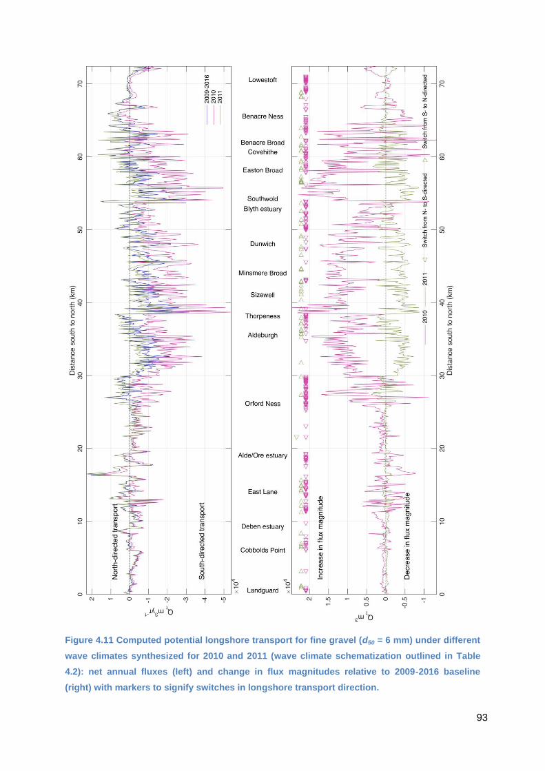
93
Figure 4.11 Computed potential longshore transport for fine gravel (d50 = 6 mm) under different
wave climates synthesized for 2010 and 2011 (wave climate schematization outlined in Table
4.2): net annual fluxes (left) and change in flux magnitudes relative to 2009-2016 baseline
(right) with markers to signify switches in longshore transport direction.

94
Given the sensitivity of wave shoaling and refraction to depth, a change in water level due to
sea-level rise might be expected to reduce the effectiveness of the offshore bank systems in
reducing wave energy at the beach. Of course, the likely changes in depth are small –
perhaps only around 0.5 m by 2100 for most ‘mid-range’ sea-level projections for the region
– and the effect of bathymetric error (van der Waal and Pye, 2003; Cea and French, 2012)
must always be borne in mind. The +0.75 m scenario modelled here thus represents likely
sea-level rise and a little margin for error.
Results from this simulation, again performed only for the 6 mm gravel fraction, are shown in
Figure 4.12. Although the changes in rate are very small in percentage terms (wave height
increase is on average < 10%), some of these do highlight the reduced effectiveness of the
nearshore banks in reducing wave energy with an increase in water depth. For example, with
a 0.75 m rise in sea level, flux magnitude increases in the vicinity of Kessingland and
Benacre Ness (where Newcome and Barnard Sands lie offshore) for both stretches of south-
directed and north-directed transport. Elsewhere, such as the alongshore varying increases
and decreases in flux between Easton Broad and Benacre Ness, the effect of increased
water depth is to slightly change the foci of high and low and north- or south-directed fluxes
and the overall spatial pattern of net fluxes appears to change very little. At Thorpeness, the
effectiveness of the subtidal platform in attenuating wave energy is reduced and sediment
fluxes increase here. The extent to which this is a realistic representation of sea-level rise
might be debated and it is unclear how bank crest elevations are adjusted to or respond to
changes in mean sea level. However, the results do corroborate other studies that argue for
the importance of the bank systems in mediating wave energy at the coast.

95
Figure 4.12 a) Computed potential longshore transport for fine gravel (d50 = 6 mm) under
contemporary wave climate (West Gabbard; Table 4.1) without and with a 0.75 m increase in
sea level imposed: net annual fluxes (left) and change in flux magnitude (right) with markers to
signify switches in longshore transport direction.

96

97
5. Applicability of the shingle engine concept to Suffolk
5.1 Review of the Dutch ‘sand engine’ concept
The Dutch ‘Zand Motor’, or ‘Sand Engine’ concept emerged from the 'Building with Nature'
national research programme, initiated in 2008 to develop new approaches to the design and
sustainable use of river, coastal and delta areas (Van Raalte et al., 2008; Van den Hoek et
al., 2012; Van Slobbe et al., 2013; de Vriend, 2013). This programme is not focused solely
on coastal defence and sediment management, but explores a wide range of morphological
and ecological manipulations that are underpinned and sustained by natural processes.
Innovation is a key aim of projects undertaken within the programme, and the ethos
promoted includes improving and increasing ecological value within both source (dredge)
and sink (nourishment) sites. This is undertaken by first seeking a clear understanding of
morphological and ecological function before large-scale landscaping to achieve ecological
enhancement.
The Sand Engine is one of several projects undertaken under 'Building with Nature'.
Although classed as a pilot project, due to the scale of the task and application it was
preceded by an earlier pilot project called the ‘Sand Groyne’. This provided a test case for
the evaluation of natural sediment redistribution (Hoekstra et al., 2012). Three Sand Groynes
comprising small sandy headlands were constructed on the upper shoreface along
approximately 2.5km of the Delfland coast in autumn 2009. A dedicated monitoring and
modelling study accompanied the construction of these headlands. Early results show that
the sandy features have been and continue to be redistributed along shore, with negligible
loss of material offshore (Hoekstra et al., 2012).
The push for development of innovative methods of 'coastal maintenance' that achieve
economic, social and conservation benefits, led to the establishment of the Sand Engine
project. The project is effectively an upscaling of the shoreface sediment replenishment
undertaken in the Sand Groyne project. Mega-nourishment projects of this kind involve
significantly larger quantities of sediment to achieve the long-term sustainability required for
economic and conservation value. Where nourishment projects already exist (i.e. where
sediment replenishment is known to be an effective solution to coastal sediment
management problems), application of a larger volume can often be more cost-effective due
economies of scale. Scheme costing can also benefit from alignment with lows in market
prices (van Dalfsen and Aarninkhof, 2009). There has also been a growing recognition that
small-scale nourishment projects, which have to be implemented on an annual to multi-
annual frequency, lead to the development of a permanent disturbance condition for many of
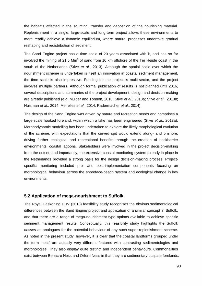
98
the habitats affected in the sourcing, transfer and deposition of the nourishing material.
Replenishment in a single, large-scale and long-term project allows these environments to
more readily achieve a dynamic equilibrium, where natural processes undertake gradual
reshaping and redistribution of sediment.
The Sand Engine project has a time scale of 20 years associated with it, and has so far
involved the mining of 21.5 Mm3 of sand from 10 km offshore of the Ter Heijde coast in the
south of the Netherlands (Stive et al., 2013). Although the spatial scale over which the
nourishment scheme is undertaken is itself an innovation in coastal sediment management,
the time scale is also impressive. Funding for the project is multi-sector, and the project
involves multiple partners. Although formal publication of results is not planned until 2016,
several descriptions and summaries of the project development, design and decision-making
are already published (e.g. Mulder and Tonnon, 2010; Stive et al., 2013a; Stive et al., 2013b;
Huisman et al., 2014; Meirelles et al., 2014; Radermacher et al., 2014).
The design of the Sand Engine was driven by nature and recreation needs and comprises a
large-scale hooked foreland, within which a lake has been engineered (Stive et al., 2013a).
Morphodynamic modelling has been undertaken to explore the likely morphological evolution
of the scheme, with expectations that the curved spit would extend along- and onshore,
driving further ecological and recreational benefits through the creation of backbarrier
environments, coastal lagoons. Stakeholders were involved in the project decision-making
from the outset, and importantly, the extensive coastal monitoring system already in place in
the Netherlands provided a strong basis for the design decision-making process. Project-
specific monitoring included pre- and post-implementation components focusing on
morphological behaviour across the shoreface-beach system and ecological change in key
environments.
5.2 Application of mega-nourishment to Suffolk
The Royal Haskoning DHV (2013) feasibility study recognises the obvious sedimentological
differences between the Sand Engine project and application of a similar concept in Suffolk,
and that there are a range of mega-nourishment type options available to achieve specific
sediment management results. Conceptually, this feasibility study highlights the Suffolk
nesses as analogues for the potential behaviour of any such super replenishment scheme.
As noted in the present study, however, it is clear that the coastal landforms grouped under
the term 'ness' are actually very different features with contrasting sedimentologies and
morphologies. They also display quite distinct and independent behaviours. Commonalities
exist between Benacre Ness and Orford Ness in that they are sedimentary cuspate forelands,

99
but Thorpe Ness is a bedrock terrestrial and submarine headland where small-scale
sedimentary accumulation is achieved due to the largely stable structural control of the
Coralline Crag here (Lees, 1980). The sedimentary similarity between Orford Ness and
Benacre Ness is also limited; Orford Ness is predominately gravel, comprising low amplitude
beach ridges, whereas Benacre Ness also incorporates low dunes due to the higher sand
content here. Moreover, the morphodynamic behaviour of these two system is entirely
different - Benacre Ness has a long history of alongshore migration and Orford Ness is by
comparison very stable. Consideration of the possible behaviour of a shingle engine as a
direct analogue of the Suffolk nesses is thus problematic.
Alternative analogues for mega-nourishment have been proposed elsewhere. For example,
Achete and Luijendijk (2012) describe the behaviour of an inlet-adjacent bar on the Ameland
coast of the Netherlands as having clear similarities with mega-nourishment projects. The
Bornrif is a large-scale swash bar that forms part of the Amelander inlet ebb delta. In its early
formation stages, it achieves a hooked spit form, which is then reshaped and redistributed by
wave processes over several years, consequently supplying the adjacent shoreline with
sediment. Separate phases of growth, extension and complete welding occur on a decadal
time-scale, and the morphologies of this evolution are similar to those seen in the Sand
Engine project.
Broadly equivalent environments exist in Suffolk. The small forelands on the south margin of
both the Deben and Alde/Ore inlets are comparable in scale and formative processes (ebb
delta bypassing). In both these cases, however, the redistribution of sediment from the small
foreland is slow and small-scale, and not necessarily directed beyond the inlet region.
Recent inlet and ebb-delta behaviour and morphology at these estuary mouths implies bi-
directional sediment movement, and the prospect of sediment delivery to the sediment-
starved shorelines to the south (Felixstowe and East Lane respectively) is quite limited.
Regional wave climate would need to change quite substantially to northeasterly dominance,
possibly with a slight shift towards a more east-northeasterly direction, for significant and
assured southerly sediment drift occur.
Royal Haskoning DHV (2013) suggest that mega-nourishment could provide significant flood
and coastal erosion risk management benefits at four candidate locations: Southwold,
Aldeburgh-Slaughden, Benacre and Felixstowe. There are some differences in the local
geomorphological context at these sites, but specifically in terms of their upper shoreface
profile and sedimentology. The shoreline at Aldeburgh and Slaughden is gravel-dominated.
Southwold, Benacre and to a lesser extent Felixstowe all have a significant sand fraction
within the intertidal and nearshore environment, due primarily to the significant supply of
sand from the Easton-Covehithe and Bawdsey cliffs (see Section 3.4 of this report).

100
The shoreface context is also of importance, and to some extent reflects the differences in
sediment matrix at the different sites. Figure 5.1 shows the shoreface profiles for these sites.
The Southwold-Benacre inshore zone (nearshore to upper shoreface) has a slope of around
1:100 (0.6°); at Felixstowe, the slope decreases to 1:200 (0.3°), where a large platform is
formed in London Clay. At Aldeburgh, the slope is notably steeper (1:65; 0.9°). Although
upper shoreface slopes in the region of the Sand Engine project are not dissimilar (c. 1:100;
0.6°), wave approach is more varied on that part of the Dutch coast, and the high wave
obliquity experienced in Suffolk is not common. Given these differences, application of large-
scale replenishment would therefore likely result in different behaviours and achieve different
benefits between the candidate locations identified by Royal Haskoning DHV (2013).
Ecological benefits of a large-scale nourishment project in Suffolk could be significant.
Suffolk already has a significant area of coastal habitats of conservation significant (Guthrie
and Cottle, 2002). Vegetated shingle in Suffolk comprises several important habitat types in
Annex I of the Habitats Directive including H1210 Annual vegetation of drift lines, H1220
Perennial vegetation of stony banks, and H1150 Coastal lagoons. Shingle features are also
associated with the development of dune habitats at locations where sand supply is
significant (e.g. Benacre Ness). It is logical to assume that this suite of habitats could
develop in the context of a mega-nourishment scheme, given similar sedimentology.
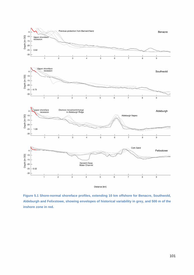
101
Figure 5.1 Shore-normal shoreface profiles, extending 10 km offshore for Benacre, Southwold,
Aldeburgh and Felixstowe, showing envelopes of historical variability in grey, and 500 m of the
inshore zone in red.

102
5.3 Recommendations for monitoring and evaluation
Successful monitoring and appraisal of coastal engineering and management schemes is
critically dependent on the ability to track change in key performance or system state
indicators. In the case of sediment nourishment schemes, this unpacks into several
overarching requirements.
Recommendation 1: As a first step, the functioning of the existing system must be
conceptualised in a way that translates into measurable indicators that can be used to track
the evolution of scheme over time and evaluate the extent to which its behaviour is as
expected, converging on anticipated endpoints, and delivering the desired functionality (in
terms of flood and erosion protection, habitat value, amenity value etc.).
With respect to the implementation of one or more shingle engines on the Suffolk coast,
Royal Haskoning DHV (2013) have undertaken valuable groundwork to scope a suite of
technical functions and articulate the ways that these might translate in diverse stakeholder
benefits. Formally translating these into indicator metrics that can inform systematic
monitoring and scheme appraisal is not entirely straightforward. The concept of the Coastal
State Indicator (CSI) is relevant here. In the words of Marchand et al. (2011), CSIs are "a
reduced set of measurable parameters that can simply, adequately, and quantitatively
describe the dynamic-state and evolutionary trends of a coastal system”. CSIs originate both
from science (often through the reductionist application of process-based models) and
society (through stakeholder knowledge and priorities). The latter set of CSIs is often in the
form of qualitative concepts directly related to a particular problem and there may be some
difficulty in achieving a perfect mapping of these onto achievable science-derived CSIs,
which are increasingly derived from model outputs. These tensions have been explored by
van Koningsveld et al. (2007) and the issue has also been revisited as part of the NERC
iCOASST project (Nicholls et al., 2012). The iCOASST work on CSIs has focused mainly on
the adoption of a participatory approach to align scientific and stakeholder needs in the
development and application of new mesoscale coastal and estuarine behaviour models
(French et al., 2016a,b). A similar argument can be extended to the formulation of monitoring
programmes, which feed directly into scheme evaluation (and possibly further intervention)
as well as into the validation and forcing of morphodynamic models. Given the scale of the
proposed shingle placements being undertaken here it would be appropriate to give serious
thought to this conceptual stage.
Recommendation 2: It is particularly important in the context of Suffolk that stakeholder
involvement is established early on. Effective management of coastal sediment systems

103
depends not only on scientific research and its ability to provide insights at the scale of
interest, but also the meshing of scientific knowledge with stakeholder knowledge and
expectations of scheme delivery. In Suffolk, large stretches of shoreline, especially north of
Southwold and around East Lane, are experiencing substantial rates of retreat, which have
led in places to ad hoc, independent (and subsequently deemed illegal) coastal protection
works (e.g. Easton Bavents - Figure 5.2). Local support would be required for the multi-
function success of a super-nourishment scheme, significant communication and
engagement would be needed throughout the decision-making process. The Sand Engine
project included significant stakeholder involvement from the outset (Van Raalte et al., 2008)
as the Building with Nature programme is underpinned by a desire to achieve societal goals
through sustainable, and wherever possible, natural solutions (van Dalfsen and Aarninkhof,
2009). The scale of the Sand Engine necessitated integrated governance, whereby decision-
making extended across the public, private, political and scientific sectors (van Slobbe et al.,
2013). Coastal management on this scale exposes the process to national and even
international attention, so the pressure to set clear requirements, goals and methods of
monitoring and assessment is high.
Figure 5.2 Easton Bavents cliffs (north of Southwold) where local landowners dumped large
quantities of soil in an attempt to retard cliff retreat. The dumped material is actively receding,
and exhibits some complicated interactions with natural cliff and beach material.

104
Recommendation 3: Once monitoring objectives and state indicators (CSIs) have been
robustly defined, detailed monitoring of coastal morphology should be undertaken to support
empirical analyses of evolving morphology as well as validate the models that allow us to
transfer our understanding into prediction of future possibilities. Although the details must
necessarily await conclusion of the conceptual process highlighted above, core elements of a
monitoring programme can readily be surmised. The dynamic behaviour of coastal sediment
systems is fundamentally manifest in changes in sediment volumes and the articulation in
landform morphological change. Coastal landforms provide a physical template that not only
accommodates diverse ecosystem functions and human activities (Murray et al., 2008), but
also mediate flood and erosion risk (Sayers et al., 2002; Narayan et al., 2012).
Systematic coastal monitoring has come a long way since the ad hoc studies that
characterised coastal geomorphology over much of the 20th century and the Suffolk coast
has a longer history of enlightened monitoring than many other parts of the UK. Key datasets
along the coast itself are the beach profile surveys undertaken by the Environment Agency
since 1991, extensive aerial photographic surveys, and coastal lidar altimetry acquired in
multiple campaigns since 1995. Surveys of offshore bathymetry have been more sporadic
and often driven by navigational or other commercial needs rather than environmental
monitoring per se. These endeavours have brought us a long way, but tackling the multiple
uncertainties that remain concerning the functioning of the Suffolk coastal sediment system
requires improvements to specific aspects of current monitoring:
Recommendation 3.1: Most important perhaps, the scale of the monitoring must match the
detailed requirements of the proposed management intervention including the models
required to evaluate its wider impact and longer-term behaviour and performance. Super-
nourishments need to be monitored in terms of local responses as well as wider impacts,
possibly at a scale of several tens of kilometres, over a time span of many decades. In the
case of the beach system, the existing Environment Agency profile monitoring provides an
excellent resource but thought should be given to finer sampling than the current 1 km
interval. In contrast, the airborne lidar campaigns have been conducted in a far more ad hoc
manner, such that regional coverages must be stitched together as a mosaic of surveys. This
frequently introduces unwelcome offsets at the boundaries and there are numerous voids.
A major issue with past airborne lidar campaigns is that the coastal surveys have seemingly
been fitted into other surveys, such that flight times coincide with arbitrary tidal states. The
intertidal zone is thus often very poorly resolved and sometimes almost entirely missed,
which makes the detection of change between successive surveys very difficult.

105
Recommendation 3.2: Timing and coordination of monitoring to align with key CSIs, such
as intertidal volume, should ideally be improved. This could be addressed in at least two
ways: 1) though prioritising coastal surveys to coincide with low tidal states in order that as
much of the intertidal as possible is captured; and 2) through the acquisition of bathymetry
lidar systems that use green as well as red lasers to resolve subtidal bathymetry. The waters
of the southern North Sea waters are typically turbid, such that the depth penetration would
be less than many other parts of the world. However, even a few metres penetration would
facilitate more seamless integration with vessel-based surveys. The nearshore zone is
possibly the least-mapped component of our coastal-shoreface environment and the data
gap between profiles, airborne Lidar data and offshore bathymetry impedes our
understanding of beach behaviour and the exchange of material between beach and
shoreface. The recently commenced Environment Agency multi-beam coastal swath surveys
will help here, but the value of these datasets could be enhanced considerably by new and/or
better-scheduled airborne altimetry and bathymetry surveys.
Recommendation 3.3: Intensive ground-based surveys should be undertaken to record
morphological changes within and adjacent to any super-nourishment. Monitoring of
morphological change within the Dutch Sand Engine project has been undertaken through
monthly intertidal and nearshore surveys using a bespoke Jet ski mounted RTK-GPS and an
echo sounder system to achieve accuracies of the order of 10 cm (Stive et al., 2013b).
Investment in surveying techniques, and the development of innovative approaches, are
features of this programme, which also includes the deployment of Argus monitoring stations.
The Argus ground-based remote sensing system comprises elevated cameras that sample at
frequencies up to 2 Hz to monitor foreshore morphology and nearshore bathymetry using
structural (image-based) properties of the wave field (Wengrove et al., 2013). Concurrent
digital panchromatic and IR photography would also greatly facilitate the mapping of both
sediments and ecological characteristics, but as shown in the Sand Engine project, other
beneficial applications (such as using IR imagery to classify beach surfaces) can emerge
through the duration of the monitoring program (Hoonhout et al., 2014).
Recommendation 3.4: Coastal oceanographic monitoring should be another priority area.
The WaveNet programme has been a step forward and continues to generate valuable
datasets. Consideration might be given to the deployment of additional offshore buoys,
although the active network in the southern North Sea is pretty good by most standards.
North Suffolk is currently well represented by the Southwold and Sizewell wave buoys, and
there is a dedicated wave buoy offshore of Felixstowe, but there is a significant mid-Suffolk
gap between East Lane and Aldeburgh. Although the West Gabbard buoy is at this latitude, it
is significantly further offshore. The wave modelling reported here shows that there are
106
significant changes and direction reversal in nearshore wave climate along this stretch that
would benefit from increased wave climate monitoring here. Monitoring of other aspects of
hydrodynamics such as tidal levels and currents are also important. The role of tidal currents
in Suffolk shoreface morphodynamics is largely derived from the morphological
characteristics of offshore banks and some early field studies (e.g. Robinson, 1966). In the
vicinity of Aldeburgh, where Aldeburgh Ridge has progressively moved onshore during the
100+ years, the function of these currents in nearshore processes is poorly understood.
Recommendation 3.5: Morphological change monitoring should be supplemented by
ecological surveys. In the Sand Engine project, considerable surveying effort has been
extended to the ecological facets of the scheme, with specific focus on dune development
(Nelisse-Rovers and Boon, 2012). More broadly, this work has been aligned with the Building
with Nature programme (van Raalte et al., 2008). Comparable efforts would be an essential
element of any mega-nourishment scheme on the Suffolk coast, but the detail of any
programme would depend on location.
Recommendation 4: Intensive modelling should be supplemented by both pre- and post-
project morphodynamic modelling. The early stages of the Dutch Sand Engine project
progressed a suite of morphodynamic models of various morphological designs, the results
of which formed the basis of the decision-making process. This included computations of
waves, flow velocity, sediment transport and sub-, inter- and supratidal morphological
change across the scheme and adjacent coastline (Mulder and Tonnon, 2010), the former of
which requiring suitable, high quality, contemporary input data. In Suffolk, HR Wallingford
(2016) have recently completed an initial model-based evaluation of the feasibility of a
shingle engine at Slaughden. This uses SWAN numerical wave model results in conjunction
with a more computationally efficient emulator to derive a 35-year time series of inshore
wave conditions. These are then used to drive a conventional one-line model (Beachplan) in
order to simulate the planform evolution of hypothetical shingle engine volumes and
configurations.
Recommendation 5: A guiding principle should be that of making all data and model outputs
freely available, readily downloadable, and widely useable via an open data policy. We are
increasingly moving from a world of closed data and models based on proprietary closed-
source software codes to one that is embracing open-source software and open data. Portals
such as the INSPIRE portal for the retrieval of UKHO hydrographic surveys, and WAVEnet
are excellent examples of this. The Sand Engine project monitoring programme generates

107
considerable volumes of data. These are stored and organised within a project-specific data
management system designed to accommodate different data types from a variety of
sources (Nelisse-Rovers and Boon, 2012). Consideration should be given to the
establishment of an open data portal for dissemination, with early planning to establish a
data management system. The Channel Coastal Observatory (http://www.channelcoast.org/)
is an excellent example of an archiving and delivery platform and the provision of data. Data
and model results are mostly made available through an Open Government licence that
encourages rather than stifles use by the broadest spectrum of researchers and stakeholders.

108

109
6. References
Achete, F., Luijendijk, A. (2012) Applying an analogue for a conceptual model for the development of a mega nourishment. Coastal Engineering Proceedings 33. Adams, N., Inman, D.L., Lovering, J.L. (2011) Effects of climate change and wave direction on longshore sediment transport patterns in Southern California. Climatic Change 109 (Suppl 1), S211-S228. Bell, J. (1836) A New and Comprehensive Gazetteer of England and Wales: Vol I. Fullarton and Co: Glasgow, 472pp. Bender, C., Dean, R. (2003) Wave field modification by bathymetric anomalies and resulting shoreline changes: a review with recent results. Coastal Engineering 49, 125-153. Booij, N., Ris, R.C., Holthuijsen, L.H. (1999) A third-generation wave model for coastal regions, part I: model description and validation. Journal of Geophysical Research 104 (C4), 7649-7666. Bradbury A.P., Mason T.E., Barter P. (2005) Large-scale multi-agency strategic beach monitoring of the South-East of England - provision of data and analytical tools. In: Proceedings of the Florida Shore and Beach Preservation Association National Conference on Beach Preservation Technology, Hilton San Destin, Florida, USA. Brooks, S.M., Spencer, T. (2010) Temporal and spatial variations in recession rates and sediment release from soft rock cliffs, Suffolk coast, UK. Geomorphology 124, 26-41. Burningham, H., French, J.R. (2006) Morphodynamic behaviour of a mixed sand-gravel ebb-tidal delta: Deben estuary, Suffolk, UK. Marine Geology 225, 23-44. Burningham, H., French, J.R. (2007) Morphodynamics and sedimentology of mixed-sediment inlets. Journal of Coastal Research SI50, 710-715. Burningham, H., French, J.R. (2009) Historical seabed mobility in an outer estuary - sea basin environment. Journal of Coastal Research SI56, 589-593. Burningham, H., French, J.R. (2014) Travelling forelands: complexities in drift and migration patterns. Journal of Coastal Research SI70, 102-108. Burningham, H. (2015) Gravel spit-inlet dynamics: Orford Spit, UK. In: Randazzo, G., Cooper, J.A.G., Jackson D., Sand and Gravel Spits, Coastal Research Library, Vol 12, Springer 300p. Burningham, H., French, J.R. (2015) Large-scale spatial variability in the contemporary coastal sand and gravel resource, Suffolk, eastern UK. In: Wang, P., Rosati, J.D., Cheng, J. (Eds.) Proceedings Coastal Sediments 2015, 15pp. Bunny, C. (2011) A high resolution SWAN model assessment: North Norfolk to Humber. Forecasting Research Technical Report 557. Met Office, Exeter, 31pp. Cambers, G. (1975) Sediment Transport and Coastal Change. East Anglian Coastal Research Programme, Report 3, University of East Anglia, Norwich, 65 pp.

110
Camden, W. (1722) Britannia or a chorographical description of Great Britain and Ireland, together with the adjacent islands: Vol I. Gibson: London, 1248pp. Carr, A.P. (1972) Aspects of spit development and decay: the estuary of the River Ore, Suffolk. Field Studies 3, 633-653 Carr, A.P. (1979) Sizewell-Dunwich Banks field study. Topic Report 2: Long-term changes in the coastline and offshore banks. Institute of Oceanographic Sciences Report 89, 30pp. Carr, A.P. (1981) Evidence for the sediment circulation along the coast of East Anglia. Marine Geology 40, M9–M22. Carr, A.P. (1986) The estuary of the River Ore, Suffolk: three decades of change in a longer- term context. Field Studies, 6, 43-58. Cea, L., French, J.R. (2012) Bathymetric error estimation for the calibration and validation of estuarine hydrodynamic models. Estuarine and Coastal Shelf Science 100, 124-132. Cooper, N.J., Jay, H. (2002) Predictions of large-scale coastal tendency: development and application of a qualitative behaviour-based methodology. Journal of Coastal Research SI36, 173-181. Cromwell, T.K. (1819) Excursions in the county of Suffolk: Vol II. Longman: London, 198pp. Coughlan, C., Vincent, C.E., Dolphin, T.J., Rees, J.M. (2007) Effects of tidal stage on the wave climate inshore of a sandbank. Journal of Coastal Research SI70, 751-756. Environment Agency (2007) Coastal trends report: Suffolk (Lowestoft to Languard Point, Felixstowe). RP003/S/2007. Environment Agency, Peterborough, 49pp. Environment Agency (2011) Coastal trends report: Suffolk (Lowestoft to Languard Point, Felixstowe). RP022/S/2011. Environment Agency, Peterborough, 46pp. Environment Agency (2013) Sea state report: Felixstowe wave buoy, 2012-2013. RP036/E/2013. Environment Agency, Peterborough, 17pp. French, J.R., Burningham, H., Thornhill, G., Nicholls, R.J. (2016a) Integrating estuarine, coastal and inner shelf sediment systems in a common conceptual framework as a basis for participatory shoreline management. In: Meadows, M., Lin, J-C. (eds.) Geomorphology and society. Singapore, Springer, 245-277. French, J.R., Burningham, H., Thornhill, G., Whitehouse, R., Nicholls, R.J. (2016b) Conceptualizing and mapping coupled estuary, coast and inner shelf sediment systems. Geomorphology 256,17-35, http://dx.doi.org/10.1016/j.geomorph.2015.10.006 Funnell, B.M. (1996) Plio-Pleistocene palaeogeography of the southern North Sea Basin (3.75–0.6 Ma). Quaternary Science Reviews 15, 391-405. Guthrie, G., Cottle, R. (2002). Suffolk Coast and Estuaries Coastal Habitat Management Plan. Posford Haskoning, Project Number 3G547201, 209pp. James, J.W.C., Lewis, P.M. (1996) Sediment input from coastal cliff erosion. Technical Report 577/4/A, Environment Agency, Peterborough, 67pp.

111
Hoekstra, R., Walstra, D.J.R., Swinkels, C.S. (2012) Pilot project Sand Groynes, Delfland coast. Coastal Engineering Proceedings, 33. Holthuijsen, L.H., Booij, N., Ris, R.C. (1993) A spectral wave model for the coastal zone, Proceedings 2nd International Symposium on Ocean Wave Measurement and Analysis, New Orleans, Louisiana, July 25-28, 1993, New York, 630-641. Hoonhout, B.M., Baart, F., Van Thiel de Vries, J.S.M. 2014. Intertidal beach classification in infrared images. Journal of Coastal Research SI70, 657-662. HR Wallingford (2016) Sandscaping Feasibility Assessment: Suffolk Shingle Engine, Slaughden Site. HR Wallingford Report DDR5443-RT001 for The Crown Estate. Huisman, B.J.A., Sirks, E.E., van der Valk, L., Walstra, D.J.R. (2014). Time and spatial variability of sediment grading in the surfzone of a large scale nourishment. Journal of Coastal Research SI70, 127-132. Kamphuis, J.W. (1991) Alongshore sediment transport rate. Journal of Waterway, Port, Coastal and Ocean Engineering 117, 624-640. Kelly, R., Hawkins, K. (2009) Suffolk Shoreline Management Plan 2. Natural and Built Environment Baseline. Royal Haskoning, Project Number 9S4195, 147pp. Koningsveld, M.V., Stive, M.J.E., Mulder, J.P.M., Vriend, H.J.d., Ruessink, B.G., Dunsbergen, D.W. (2003) Usefulness and Effectiveness of Coastal Research: A Matter of Perception? Journal of Coastal Research 19, 441-461. Laustraup, C.T., Madsen, H.B., Knudsen, S., Sørensen, P. (2000) Coastal steepening in Denmark. Proceedings Coastal Engineering 2000, Volume 3. American Society of Civil Engineers (ASCE), Sydney, 2428–2438. Lees, B.J. (1980) Sizewell - Dunwich Banks Field Study. Topic Report 1: Introduction and Geological Background. Institute of Oceanographic Sciences, Report No. 88, 45pp. Madsen, O.S., Poon, Y-K. Graber, H.C. (1988) Spectral wave attenuation by bottom friction: theory. Proceedings 21st International Conference on Coastal Engineering. American Society of Civil Engineers, 492-504. Marchand, M., Sanchez-Arcilla, A., erreira, M., Gault, ., im nez, .A., Markovic, M., Mulder, ., van Ri n, ., St nic , A., Sulisz, W. (2011) Concepts and science for coastal erosion management–An introduction to the Conscience framework. Ocean & Coastal Management 54, 859-866. McCave, I.N. (1987) Fine sediment sources and sinks around the East Anglian coast (UK). Journal of the Geological Society of London 144, 149-152. Meirelles, S., Horner-Devine, A.R., Henriquez, M., Stive, M., Pietrzak, J., Souza, A.J. (2014) Middle shoreface sand transport under stratified regimes. Journal of Coastal Research SI70, 182-186. Mulder, J.P.M., Tonnon, P.K. (2010) 'Sand engine': background and design of a mega-nourishment pilot in the Netherlands. Coastal Engineering Proceedings, 32. Montreuil, A-L., Bullard J.E. (2012) A 150-year record of coastline dynamics within a sediment cell: Eastern England. Geomorphology 179, 168-185.

112
Motyka, J.M., Beven, S.M. (1987) A macro review of the coastline of England and Wales. Volume 3: The Wash to the Thames. HR Wallingford Report SR 135, 113pp. Murray, A.B., Lazarus, E., Ashton, A., Baas, A., Coco, G., Coulthard, T., Fonstad, M., Haff, P.K., McNamara, D., Paola, C., Reinhardt, L. (2008) Geomorphology, complexity, and the emerging science of the Earth‘s surface. Geomorphology 103, 496-505. Nelisse-Rovers, I., Boon, A. (2012) The Sand Engine – a sustainable coastal appendix. In: Belpaeme, K. et al. (Ed.) Book of Abstracts. International Conference Littoral 2012: Coasts of Tomorrow. VLIZ Special Publication, 61, 150-152. Narayan, S., Hanson S., Nicholls, R.J., Clarke, D., Willems, P., Ntegeka, V., Mobaliu, J. (2012) A holistic model for coastal flooding using system diagrams and the source-pathway- receptor (SPR) concept. Natural Hazards and Earth System Science 12, 1431-1439. Nicholls, R.J., Bradbury, A., Burningham, H., Dix, J., Ellis, M., French, J., Hall, J.W., Karunarathna, H.U., Lawn, J., Pan, S., Reeve, D.E., Rogers, R., Souza, A., Stansby, K., Sutherland, J., Tarrant, O., Walkden, M., Whitehouse, R. (2012) iCOASST - integrating coastal sediment systems. Coastal Engineering Proceedings 1(33). 100. Nicholls, R.J., Wright, P. (1991) Longshore transport of pebbles: experimental estimates of K-factor. Proceedings Coastal Sediments 1991, Volume 2, 1563-1577. Onyett, D. Simmons, A. (1983) East Anglian Coastal Research Project Final Report, Geobooks, Norwich, 125 pp. Pontee, N.I. (2005) Management implications of coastal change in Suffolk, UK. Proceedings of the Institution of Civil Engineers. Maritime Engineering 158, 69-83. Pontee, N.I. (2013) Defining coastal squeeze: a discussion. Ocean & Coastal Management 84, 204-207. Pontee, N.I., Pye, K., Blott, S.J. (2004) Morphodynamic behaviour and sedimentary variation of mixed sand and gravel beaches, Suffolk, UK. Journal of Coastal Research 20, 256-276. Pye, K., Blott, S.J. (2006) Coastal processes and morphological change in the Dunwich-Sizewell area, Suffolk, UK. Journal of Coastal Research 22, 453-473. Pye, K., Blott, S.J. (2009) Progressive breakdown of a gravel-dominated coastal barrier, Dunwich-Walberswick, Suffolk, UK: processes and implications. Journal of Coastal Research 25, 589-602. Quinn, J.D., Philip, L.K., Murphy, W. (2008) Understanding the recession of the Holderness Coast, east Yorkshire, UK: a new presentation of temporal and spatial patterns. Quarterly Journal of Engineering Geology and Hydrogeology 42, 165-178. Radermacher, M., Wengrove, M.E., Van Thiel de Vries, J.S.M., Holman, R.A. (2014) Applicability of video-derived bathymetry estimates to nearshore current model predictions. Journal of Coastal Research SI70, 290-295. Redman, J.B. (1864) The east coast between the Thames and the Wash estuaries. Minutes of the Proceedings of the Institution of Civil Engineers 23, 186-256.

113
Robinson, A.H.W. (1966) Residual currents in relation to shoreline evolution of the East Anglian coast. Marine Geology 5, 57-84. Robinson, A.H.W. (1980) Erosion and accretion along part of the Suffolk coast of East Anglia, England. Marine Geology 37, 133-146. Royal Haskoning (2010) Suffolk SMP2 Sub-cell 3c Policy Development Zone 6 – Orford Ness to Cobbold’s Point, Suffolk Coastal District Council/Waveney District Council/ Environment Agency, 66pp & Appendices. Royal Haskoning DHV (2013) Suffolk shingle engine: Technical feasibility assessment. Crown Estate Report 9Y1362, 80pp. Sayers, P.B., Hall, J.W., Meadowcroft, I.C. (2002) Towards risk-based flood hazard management in the UK. Proceedings of the Institution of Civil Engineers 150, 36-42. SNSSTS (2002) Southern North Sea Sediment Transport Study, Phase 2. HR Wallingford, Report EX4526, Wallingford. Spencer, T., Brooks, S.M. (2012) Methodologies for measuring and modelling change in coastal saline lagoons under historic and accelerated sea-level rise, Suffolk coast, eastern England. Hydrobiologia DOI 10.1007/s10750-012-1089-x. Steers, J.A. (1926) Orfordness: a study in coastal physiography. Proceedings of the Geologists’ Association 37, 306-325. Steers, J.A. (1927) The East Anglian coast. Geographical Journal 69, 24-43. Stive, M.J.F. de Schipper, M.A. Luijendijk, A.P. Aarninkhof, S.G.J. van Gelder-Maas, C. van Thiel de Vries, J.S.M. de Vries, S. Henriquez, M. Marx, S., Ranasinghe, R. (2013a) A new alternative to saving our beaches from local sea-level rise: the sand engine. Journal of Coastal Research 29, 1001-1008. Stive, M.J.F., De Schipper, M.A., Luijendijk, A.P., Ranasinghe, R.W.M.R.J.B., Van Thiel De Vries, J.S.M., Aarninkhof, S., Van Gelder-Maas, C., De Vries, S., Henriquez, M., Marx, S. (2013b) The sand engine: A solution for vulnerable deltas in the 21st century? Coastal Dynamics Proceedings, 7. Sutherland, J., Wolf, J.A. (2002) Coastal defence vulnerability 2075. HR Wallingford Report SR 590, Wallingford, HR Wallingford. Taylor, J.A., Murdoch, A.P., Pontee, N.I. (2004) A macroscale analysis of coastal steepening around the coast of England and Wales. Geographical Journal 170, 179-188. Titus, J.G. (1991) Greenhouse effect and coastal wetland policy: How Americans could abandon an area the size of Massachusetts at minimum cost. Environmental Management 15, 39-58. Tomasicchio, G.R., D'Alessandro, Barbaro, G., Malara, G. (2013) General longshore transport model. Coastal Engineering 71, 28–36. Townend, I., McLaren, P. 1988. Anglian Coastal Management Atlas. The Anglian Sea Defence Management Study - Stage II. Sir William Halcrow and Partners, Swindon, UK, Report No: Report for Anglian Water, 1-107.

114
Townend, I., Fleming, C., McLaren, P., Hunter-Blair, A. (1990) A regional study of coastal morphology. Proceedings 22nd International Conference of Coastal Engineering, Volume 3 (197), American Society of Civil Engineers (ASCE), Delft, 2589-2602. UKHO. (1869) North Sea Pilot: Part III East Coast of England. Admiralty, 270pp. UKHO (2014) Admiralty Tide Tables. Volume 1: United Kingdom and Ireland (including European Channel Ports). U.S. Army Corps of Engineers (1984) Shore Protection Manual. U.S. Army Corps of Engineers Research and Development Center. Coastal and Hydraulics Laboratory, Vicksburg. van Dalfsen, J.A., Aarninkhog, S.G.J. (2009) Building with Nature: Mega nourishments and ecological landscaping of extraction areas. Proceedings of the EMSAGG Conference, 5-6 February 2009, Rome, Italy. van den Hoek, R.E., Brugnach, M., Hoekstra, A.Y. (2012) Shifting to ecological engineering in flood management: Introducing new uncertainties in the development of a building with nature pilot project. Environmental Science Policy 22, 85-99. Van Maanen, B., Nicholls, R.J., French, J.R., Barkwith, A., Bonaldo, D., Burningham, H., Murray, A.B., Payo, A., Sutherland, J., Thornhill, G., Townend, I.H., van der Wegen, M., Walkden, M.J.A. (2016) Simulating mesoscale coastal evolution for decadal coastal management: A new framework integrating multiple, complementary modelling approaches. Geomorphology 256, 68-80. http://dx.doi.org/10.1016/j.geomorph.2015.10.026 Van Raalte, G., Dirks, W., Minns, T., van Dalfsen, J., Erftermeijer, P., Aarninkhof, S., Otter, H. (2008) Building with nature: creating sustainable solutions for marine and inland water constructions. New research initiative towards a Centre of Excellence. Proceedings of the Eighteenth World Dredging Congress (WODCON XVIII), May 27 - June 1, 2007. Lake Buena Vista, Florida USA, pp. 637-648. van Rijn, L.C. (2014) A simple general expression for longshore transport of sand, gravel and shingle. Coastal Engineering 90, 23-39. van Slobbe, E., de Vriend, H. J., Aarninkhof, S., Lulofs., S., de Vries, M., Dircke, P. (2013) Building with nature: in search of resilient storm surge protection strategies. Natural Hazards 65, 947-966. van der Waal, D., Pye, K. (2003) The use of historical bathymetric charts in a GIS to assess morphological change in estuaries. Geographical Journal 169, 21-31. de Vriend, H. (2013) Building with Nature: towards sustainable hydraulic engineering. Proceedings of 2013 IAHR World Congress. Wengrove, M.E., Henriquez, M., de Schipper, M.A., Holman, R., Stive, M.J.F. (2013) Monitoring morphology of the Sand Engine leeside using Argus’ cBathy. Coastal Dynamics Proceedings, 7.
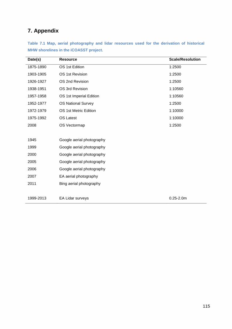
115
7. Appendix
Table 7.1 Map, aerial photography and lidar resources used for the derivation of historical
MHW shorelines in the iCOASST project.
Date(s) Resource Scale/Resolution
1875-1890 OS 1st Edition 1:2500
1903-1905 OS 1st Revision 1:2500
1926-1927 OS 2nd Revision 1:2500
1938-1951 OS 3rd Revision 1:10560
1957-1958 OS 1st Imperial Edition 1:10560
1952-1977 OS National Survey 1:2500
1972-1979 OS 1st Metric Edition 1:10000
1975-1992 OS Latest 1:10000
2008 OS Vectormap 1:2500
1945 Google aerial photography
1999 Google aerial photography
2000 Google aerial photography
2005 Google aerial photography
2006 Google aerial photography
2007 EA aerial photography
2011 Bing aerial photography
1999-2013 EA Lidar surveys 0.25-2.0m
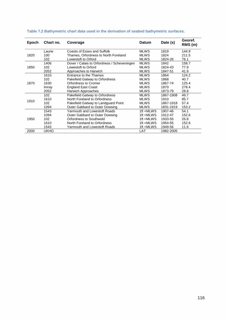
116
Table 7.2 Bathymetric chart data used in the derivation of seabed bathymetric surfaces.
Epoch Chart no. Coverage Datum Date (s) Georef. RMS (m)
1820 Laurie Coasts of Essex and Suffolk MLWS 1819 144.9 100 Thames, Orfordness to North Foreland MLWS 1824 211.5 102 Lowestoft to Orford MLWS 1824-26 76.1
1850 1406 Dover / Calais to Orfordness / Scheveningen MLWS 1842 158.7 102 Lowestoft to Orford MLWS 1824-43 77.9 2052 Approaches to Harwich MLWS 1847-51 41.9
1870
1610 Entrance to the Thames MLWS 1864 124.2 102 Pakefield Gatway to Orfordness MLWS 1868 40.7 1630 Orfordness to Cromer MLWS 1867-74 125.4 Imray England East Coast MLWS 1870 278.4 2052 Harwich Approaches MLWS 1873-79 28.8
1910
102 Pakefield Gatway to Orfordness MLWS 1867-1908 49.7 1610 North Foreland to Orfordness MLWS 1910 85.7 102 Pakefield Gatway to Landguard Point MLWS 1867-1918 57.4 1094 Outer Gabbard to Outer Dowsing MLWS 1831-1919 153.2
1950
1543 Yarmouth and Lowestoft Roads 1ft <MLWS 1907-46 54.1 1094 Outer Gabbard to Outer Dowsing 1ft <MLWS 1912-47 152.6 102 Orfordness to Southwold 1ft <MLWS 1933-55 26.8 1610 North Foreland to Orfordness 1ft <MLWS 1954-55 152.6 1543 Yarmouth and Lowestoft Roads 1ft <MLWS 1949-56 11.6
2000 UKHO LAT 1982-2005

117
Table 7.3 UKHO surveys (via INSPIRE portal) used in construction of 50 m bathymetric grid.
Date Code Description
1982 HI11 East Coast Southwold CrossSand Sheet1 1982 HI11 East Coast Southwold CrossSand Sheet2 1983 HI126 Newarp to East Cross Sand 1984 HI196 Orfordness Southwold North 1984 HI196 Orfordness Southwold South 1984 HI193HI194 Thames Estuary 1985 HI197 Approaches to Blackwater/Crouch 1987 HI345 Southern North Sea - South Falls 1988 HI414-HI420 Long Sand Head - Black Deep 1988 HI423 Kentish Knock 1988 HI421 Gunfleet Sand to the Naze 1989 HI481 Knock Deep Blk1 1989 HI481 Knock Deep Blk2 1992 HI564 South Eastern Approaches to Southwold 1993 HI572 North Shipwash 1993 HI569 Middle Scroby Winterton 1994 HI616 Smiths Knoll Orfordness Blk A020 1994 HI616 Smiths Knoll Orfordness Blk A015 1994 HI575 Rough Shoals 1994 HI616 Smiths Knoll Orfordness Blk A018 1994 HI628 Kings Channel 1994 HI616 Smiths Knoll Orfordness Blk A014 1994 HI616 Smiths Knoll Orfordness Blk A013 1994 HI616 Smiths Knoll Orfordness Blk A019 1994 HI616 Smiths Knoll Orfordness Blk A017 1994 HI616 Smiths Knoll Orfordness Blk A011 1994 HI616 Smiths Smiths Knoll to Ordford Ness Blk007 1994 HI616 Smiths Smiths Knoll to Ordford Ness Blk012 1994 HI616 Smiths Smiths Knoll to Ordford Ness Blk014 1994 HI616 Smiths Smiths Knoll to Ordford Ness Blk008 1994 HI616 Smiths Smiths Knoll to Ordford Ness Blk010 1994 HI616 Smiths Smiths Knoll to Ordford Ness Blk009 1995 HI667 Orfordness North Foreland Blk5 1995 HI667 Orfordness North Foreland Blk2 1995 HI667 Orfordness North Foreland Blk8 1995 HI652HI655HI659 Long Sand Head Black Deep 1995 HI667 Orfordness North Foreland Blk6 1995 HI667 Orfordness North Foreland Blk7 1995 HI667 Orfordness North Foreland Blk4 1995 HI667 Orfordness North Foreland Blk3 1995 HI667 Orfordness North Foreland Blk9 1995 HI667 Orfordness North Foreland Blk10 1995 HI667 Orfordness North Foreland Blk1 1995 HI661-672 Winterton Newarp Banks 1996 HI689 North Shipway 1996 HI690 Shipwash Black Deep Blk2 1996 HI690 Shipwash Black Deep Blk1 1997-2006 357614 Harwich Haven Medusa Channel 1997 H693 Kentish Knock 1997 HI733 Corton Sand 1999 HI847 Cross Sands 1999 HI844 Cockle Gateway 1999 HI848 Roads Holm Channel 2002 HI999 Lowestoft approaches 2004 H1077 Pakefield Road Blk2 2004 H1077 Pakefield Road Blk1 2006 HI1164 Approaches to Lowestoft


London The Crown Estate 16 New Burlington Place London W1S 2HX T 020 7851 5000
Edinburgh The Crown Estate 6 Bell’s Brae Edinburgh EH4 3BJ T 0131 260 6070
Glenlivet Main Street Tomintoul Banffshire AB37 9EX T 01479 870 070
Windsor The Crown Estate The Great Park Windsor, Berkshire SL4 2HT T 01753 860 222
www.thecrownestate.co.uk @TheCrownEstate
ISBN: 978-1-906410-76-6


