Short Communication Reservoir Performance Assessment … · Reservoir Performance Assessment Based...

69A. Farzamnia et al. / Journal of Chemical and Petroleum Engineering, 50 (1), Jun. 2016 / 69-78

Reservoir Performance Assessment Basedon Intelligent Well Technology

Amir Farzamnia1, Jamshid Moghadasi1*,Turaj Behrouz2 and Amir Abbas Askari2

1. Petroleum University of Technology, Iran.2. Research Institute of Petroleum Industry (RIPI), Iran.

(Received 28 September 2014, Accepted 11 December 2015)

Abstract

The main challenge facing the oil industry is to reduce development costs while accelerating recovery with maximizing reserves. One of the key enabling technologies in this area is intelligent well completions. Intelligent well technology (IWT) is a relatively new technology that has been adopted by many operators in recent years to improve oil and gas recovery. Intelligent well completions employ Annular Flow Con-trol Valves (AFCVs) to balance the production profile along the length of the well completion by splitting it into two (or more) sections. The aim of intelligent wells is to optimize the production (Delaying the gas and water breakthrough and decreasing water production).

The energy that moves crude oil and natural gas from the subsurface rock to the production well is called the reservoir drive [1]. These en-ergies because of their different mechanisms, have different effects on reservoir production. In spite of advancement in Intelligent Well Tech-nology, the effect of intelligent well on reservoir drive mechanisms un-der different reservoir characterization have not been well addressed. In this paper, six conceptual models of oil reservoir have been built and different production scenarios have been discussed. Based on the objective function, scenarios will be selected and will compare with a conventional scenario and decide whether to use smart well in these models or not.

Keywords

Annular flow control valves;Drive mechanisms; Intelligent Well Technology.

Introduction1

* Corresponding Author.Tel: +98-61-55555557; E-mail: [email protected]

Introduction

With the developments in drilling technolo-gy, long horizontal, high angle and multi-lateral wells are providing a necessary

platform to increase productivity per well and de-crease the number of wells necessary to develop an asset. Intelligent well technology (IWT) provides the suitable platform for an engineer to achieve this

objective. With this technology, the engineer can more effectively monitor the conditions by using downhole permanent sensors, and control the flow of fluids into and out of the wellbore using Annular flow Control Valves (AFCVs) on demand without physical intervention. AFCVs enable the control-ling of each valve individually from the surface to maximize oil production and/or minimize forma-tion water and/or gas production. There are three main types of AFCVs in terms of the style of con-trol: two position valves (open or close), multiple

Short Communication

70 A. Farzamnia et al. / Journal of Chemical and Petroleum Engineering, 50 (1), Jun. 2016 / 69-78

step valves and infinitely variable valves. The two position AFCV is either fully open or fully closed. The multiple step AFCVs are constructed in various designs with typically 4 to >10 steps for the choke settings as it changes from the fully open to the fully closed position. The infinitely variable AFCV has the flexibility to provide optimum control (al-ways assuming that it was placed to cover the most appropriate sections / length of the wellbore). Not surprisingly, variable AFCVs are more expensive and require more sophisticated control algorithms than the simpler types of AFCV [2]. The benefits of IWT are established in a number of previous re-searches based on reservoir simulation and case studies. These include control of multiple zone in-telligent well to meet production optimization re-quirements [3], improved reservoir management [4,5], manual optimization of valve apertures with applications in water flooding [6], optimization of Intelligent Wells – A Field Case Study [7]. Elmsallati et al worked on a case study Value Generation with IWT in a High Productivity, Thin Oil Rim Reservoir and discussed the added values of IWT [8]. In spite of advancement in IWT, the effects of intelligent wells on unwanted fluid production reduction un-der different reservoir characterization and pro-duction mechanisms have not been well addressed.

Water production is one of the major technical, environmental, and economical problems associ-ated with oil and gas production. Water produc-tion can limit the productive life of the oil and gas wells and can cause severe problems including corrosion of tubular, fines migration, and hydro-static loading. Produced water represents the larg-est waste stream associated with oil and gas pro-duction. In the United States, it is estimated that on average 8 barrels of water are produced for each barrel of oil [9]. The environmental impact of han-dling, treating and disposing of the produced wa-ter can seriously affect the profitability of oil and gas production. The annual cost of disposing the produced water in the United States is estimated to be 5-10 billion dollars [10]. Numerous technolo-gies are available for controlling unwanted water production so this problem has been resolved by appropriate reservoir management.

One approach for using intelligent well tech-nology is to react to production problems (e.g., water coning) and then reset the instrumentation to mitigate them (reactive control strategy). A bet-ter approach is to use AFCVs in conjunction with a predictive reservoir model. This allows for the optimization of reservoir performance rather than just the correction of problems that have already occurred [11].

2. Methodology

In the first step, a conceptual oil reservoir model is built. The reservoir model contains 59x59x10 grid cells in X, Y and Z directions, respectively; i.e., a total of 34810 cells. That model has 100 ft thick-ness; in the other words, the dimensions of model are 2000 ft x 2000 ft x 100 ft and upper layer of reservoir was set at 8940 ft.

2.1 Problem statementThe purpose of implementation of Intelligent Well Technology is to improve the reservoir perfor-mance. In this paper, reservoirs under different production mechanisms are studied with IWT. In various case studies, the objective function is dif-ferent. If the reservoir produced water from the aquifer, the objective function would be cumula-tive water production reduction. If the reservoir produced gas from gas cap, the objective function would be cumulative gas production reduction. If the reservoir produced water and gas, the objec-tive function would be cumulative water produc-tion reduction.

2.2 Reservoir Static ModelingIn the second step, Static properties of the model are defined. Because of applying different reser-voir characterizations, two types of reservoirs are defined: homogenous and heterogeneous.

In the homogenous model, the permeability in the X and Y directions are equal and between 27.7 and 65.4 mD and its average is 48.6 mD with Kv/KH = 0.1 (Figure 1). The porosity range is between 0.07 and 0.22 and its average is 0.15. In the het-erogeneous model, heterogeneity is applied by the channel that crosses the reservoir. The following amendments are made to introduce heterogeneity (Figure 2): Grid cells:For 1 - 9 x 59 x 10 (x, y, z), permeability is 48.6 mD and porosity 0.15For 10 – 18 x 59 x 10 (x, y, z), permeability is 486 mD and porosity 0.25For 19 – 59 x 59 x 10 (x, y, z), permeability is 48.6 mD and porosity 0.15

In the homogenous type, reservoir rock type is sandstone. In the heterogeneous type, main rock type is sandstone, and rock type of channel that crosses the reservoir, is unconsolidated sandstone.

2.3 Reservoir Dynamic ModelingIn this section, different production mechanisms are applied to reservoir models. So, according to


Figure 2. Permeability distribution in heterogeneous mod-els.

Figure 1. Permeability distribution in homogenous mod-els.

production mechanisms [12], four different pro-duction mechanisms are applied to reservoir mod-els. The used models are as below:

Model I: Homogenous, Water DriveModel II: Homogenous, Gas Cap DriveModel III: Homogenous, Solution Gas DriveModel IV: Homogenous, Combination DriveModel V: Heterogeneous, Water DriveModel VI: Heterogeneous, Combination Drive

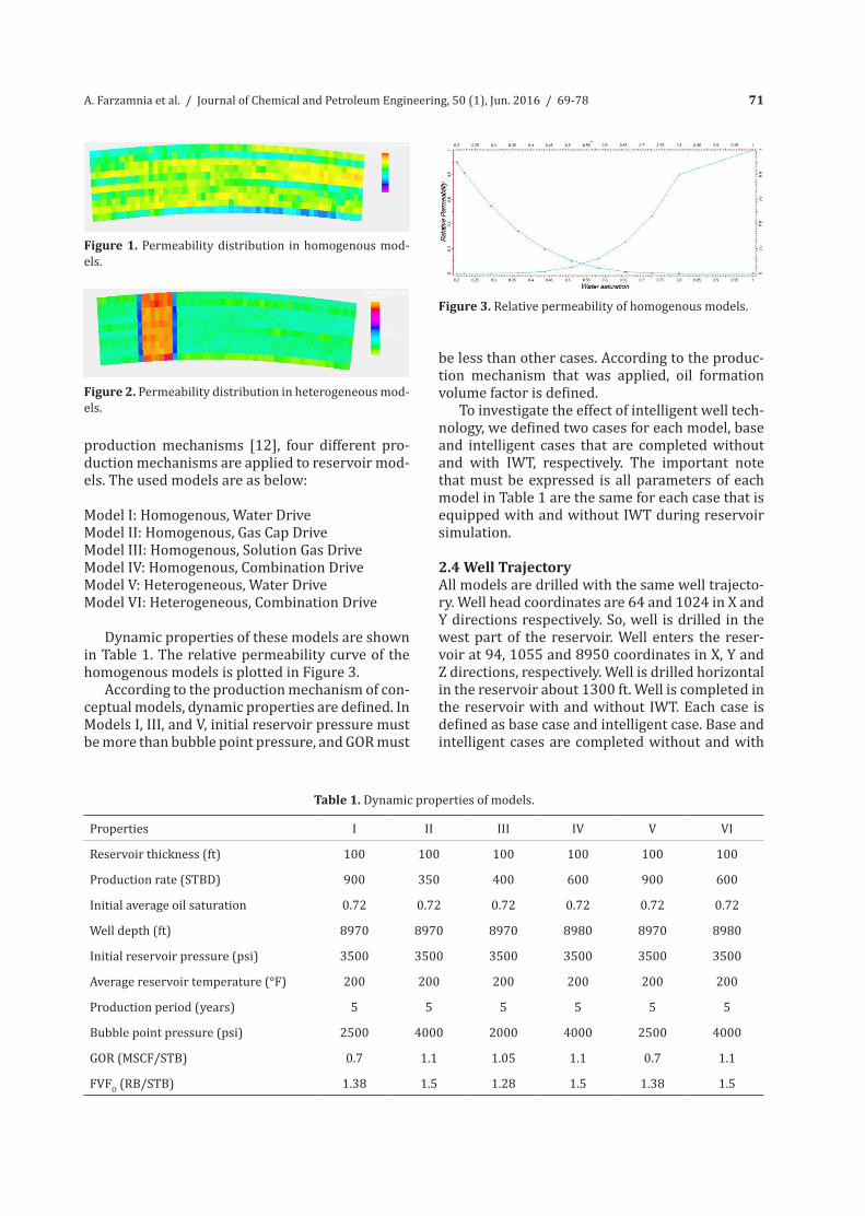
Dynamic properties of these models are shown in Table 1. The relative permeability curve of the homogenous models is plotted in Figure 3.

According to the production mechanism of con-ceptual models, dynamic properties are defined. In Models I, III, and V, initial reservoir pressure must be more than bubble point pressure, and GOR must

be less than other cases. According to the produc-tion mechanism that was applied, oil formation volume factor is defined.

To investigate the effect of intelligent well tech-nology, we defined two cases for each model, base and intelligent cases that are completed without and with IWT, respectively. The important note that must be expressed is all parameters of each model in Table 1 are the same for each case that is equipped with and without IWT during reservoir simulation.

2.4 Well TrajectoryAll models are drilled with the same well trajecto-ry. Well head coordinates are 64 and 1024 in X and Y directions respectively. So, well is drilled in the west part of the reservoir. Well enters the reser-voir at 94, 1055 and 8950 coordinates in X, Y and Z directions, respectively. Well is drilled horizontal in the reservoir about 1300 ft. Well is completed in the reservoir with and without IWT. Each case is defined as base case and intelligent case. Base and intelligent cases are completed without and with

Figure 3. Relative permeability of homogenous models.

VIVIVIIIIIIProperties

100100100100100100Reservoir thickness (ft)

600900600400350900Production rate (STBD)

0.720.720.720.720.720.72Initial average oil saturation

898089708980897089708970Well depth (ft)

350035003500350035003500Initial reservoir pressure (psi)

200200200200200200Average reservoir temperature (°F)

555555Production period (years)

400025004000200040002500Bubble point pressure (psi)

1.10.71.11.051.10.7GOR (MSCF/STB)

1.51.381.51.281.51.38FVFO (RB/STB)

Table 1. Dynamic properties of models.


In this model, production mechanism is water drive. The aquifer is set at the bottom of the reservoir and sweeps oil to bore hole. The horizontal well drilled in the reservoir is completed in the intelligent case with three AFCVs (Figure 4). The “heel-toe” effect leads to a difference in the specific influx rate between the heel and the toe of the well (Al-Khelaiwi et al. 2008). According to this effect in horizontal wells, AFCVs are set in the heel and toe of the well. AFCV1 is set in the heel of the well and AFCV2 in the middle of well and AFCV3 at the end of the well in the reservoir. As Figures 5 and 6 illustrate, at the heel of the well, water raises more than other parts of the well in the base case, and this cause water breakthrough. But in the intelligent case, by shutting the AFCV1 that is placed at the heel of the well, water breakthrough is delayed, and water is raised in other parts of the well. By controlling the AFCVs (Table 2), until the end of assumed production time, cumulative water production is decreased. As shown in Table 2, number 1 is ascribed to fully opened position of AFCV, number 0 is ascribed to fully closed position and other positions are ascribed by numbers in the range of (0,1). The cumulative water production and cumulative oil production in the base case (dashed line) and intelligent case (solid line) are plotted in Figures 7 and 8. As Figures 7 and 8 illustrate, while the cumulative oil production is fixed at a constant value in both base and intelligent cases, the cumulative water production is reduced. Reduction of cumulative water

production significantly reduces the cost of field operations. According to Table 2, during production time, AFCV1 that is set in the heel of the well is being closed. So, oil production increases in other parts of the reservoir. So breakthrough was delayed and this phenomenon causes cumulative water production in intelligent case to be less than the base case. By controlling AFCV1, the effect of breakthrough phenomenon and respectively water production, decreases. Table 3 shows the changes of water/oil cumulative production for Model I, with and without IWT. In Table 3, below equation is applied:

% 𝐷𝐷𝐷𝐷𝐷𝐷𝐷𝐷𝐷𝐷𝐷𝐷𝐷𝐷𝐷𝐷𝐷𝐷𝐷𝐷 = 𝐼𝐼𝐷𝐷𝐼𝐼𝐷𝐷𝐼𝐼𝐼𝐼𝐷𝐷𝐼𝐼𝐷𝐷𝐷𝐷𝐼𝐼 − 𝐵𝐵𝐵𝐵𝐵𝐵𝐷𝐷𝐵𝐵𝐵𝐵𝐵𝐵𝐷𝐷 × 100

As seen in Table 3, cumulative water production is reduced by 6.37 % using IWT. The homogeneous water drive reservoir achieved this reduction, because of the active aquifer that exists at the bottom of the reservoir. This aquifer maintains the pressure of the reservoir and controls water production after breakthrough. By using IWT, high influx in the heel of the well does not occur. This creates a balanced inflow throughout the well and eliminates the heel-toe effect. In addition, by controlling water rising from the aquifer, breakthrough occurs later, so cumulative water production reduces and reservoir performance improves.

Figure 4: Well Schematic Figure 4. Well Schematic.

Time AFCV1 AFCV2 AFCV3

2014-06-01 1 1 1

2017-09-01 0 1 0.5

2018-06-01 0 0.5 1

2018-12-01 1 1 1

Table 2. AFCVs conditions during production time of mod-el I.

IWT. We have two kinds of completion, the intel-ligent and basic completion. The first one with 6 5/8 inches casing and 5 inches tubing completed by IWT, and the second one which has 6 5/8 inches is not completed.

2.5 Strategy developmentSimulation of all models is started on 01.06.2014 and will be finished 5 years later on 01.06.2019. Two types of limitations are defined. First one is based on oil production rate. Table 1 shows pro-duction rate limitations in each model. The other limitation is the bottom hole pressure that is set as 1500 psi for all models. According to the reser-voir initial pressure and the bubble point pressure of the cases that were expressed in Table 1, bot-tom hole pressure limitation is set at 1500 psi. It must be less than the values of initial pressure. The first limitation stabilizes the oil production rate and does not permit an increase from that value at simulation time. By the second limitation, if the bottom hole pressure reduces from the set value, the well will be closed.

Results and Discussion

3.1 Model I: Homogenous, Water DriveIn this model, production mechanism is water drive. The aquifer is set at the bottom of the res-ervoir and sweeps oil to bore hole. The horizon-tal well drilled in the reservoir is completed in the intelligent case with three AFCVs (Figure 4). The “heel-toe” effect leads to a difference in the spe-cific influx rate between the heel and the toe of the well [13]. According to this effect in horizontal wells, AFCVs are set in the heel and toe of the well. AFCV1 is set in the heel of the well and AFCV2 in the middle of well and AFCV3 at the end of the well in the reservoir.

As Figures 5 and 6 illustrate, at the heel of the well, water raises more than other parts of the well in the base case, and this cause water break-through. But in the intelligent case, by shutting the AFCV1 that is placed at the heel of the well, wa-ter breakthrough is delayed, and water is raised in other parts of the well. By controlling the AFCVs (Table 2), until the end of assumed production time, cumulative water production is decreased.

As shown in Table 2, number 1 is ascribed to fully opened position of AFCV, number 0 is as-cribed to fully closed position and other positions are ascribed by numbers in the range of (0,1).

The cumulative water production and cumula-tive oil production in the base case (dashed line)

Figure 5. Water saturation in base case of Model I at three and a half years later.

Figure 6. Water saturation in intelligent case of Model I at three and a half years later.

and intelligent case (solid line) are plotted in Fig-ures 7 and 8. As Figures 7 and 8 illustrate, while the cumulative oil production is fixed at a constant value in both base and intelligent cases, the cumu-lative water production is reduced. Reduction of cumulative water production significantly reduces the cost of field operations.

According to Table 2, during production time, AFCV1 that is set in the heel of the well is being closed. So, oil production increases in other parts of the reservoir. So breakthrough was delayed and this phenomenon causes cumulative water pro-duction in intelligent case to be less than the base case. By controlling AFCV1, the effect of break-through phenomenon and respectively water pro-duction, decreases.


In this model, production mechanism is water drive. The aquifer is set at the bottom of the reservoir and sweeps oil to bore hole. The horizontal well drilled in the reservoir is completed in the intelligent case with three AFCVs (Figure 4). The “heel-toe” effect leads to a difference in the specific influx rate between the heel and the toe of the well (Al-Khelaiwi et al. 2008). According to this effect in horizontal wells, AFCVs are set in the heel and toe of the well. AFCV1 is set in the heel of the well and AFCV2 in the middle of well and AFCV3 at the end of the well in the reservoir. As Figures 5 and 6 illustrate, at the heel of the well, water raises more than other parts of the well in the base case, and this cause water breakthrough. But in the intelligent case, by shutting the AFCV1 that is placed at the heel of the well, water breakthrough is delayed, and water is raised in other parts of the well. By controlling the AFCVs (Table 2), until the end of assumed production time, cumulative water production is decreased. As shown in Table 2, number 1 is ascribed to fully opened position of AFCV, number 0 is ascribed to fully closed position and other positions are ascribed by numbers in the range of (0,1). The cumulative water production and cumulative oil production in the base case (dashed line) and intelligent case (solid line) are plotted in Figures 7 and 8. As Figures 7 and 8 illustrate, while the cumulative oil production is fixed at a constant value in both base and intelligent cases, the cumulative water production is reduced. Reduction of cumulative water

production significantly reduces the cost of field operations. According to Table 2, during production time, AFCV1 that is set in the heel of the well is being closed. So, oil production increases in other parts of the reservoir. So breakthrough was delayed and this phenomenon causes cumulative water production in intelligent case to be less than the base case. By controlling AFCV1, the effect of breakthrough phenomenon and respectively water production, decreases. Table 3 shows the changes of water/oil cumulative production for Model I, with and without IWT. In Table 3, below equation is applied:

% 𝐷𝐷𝐷𝐷𝐷𝐷𝐷𝐷𝐷𝐷𝐷𝐷𝐷𝐷𝐷𝐷𝐷𝐷𝐷𝐷 = 𝐼𝐼𝐷𝐷𝐼𝐼𝐷𝐷𝐼𝐼𝐼𝐼𝐷𝐷𝐼𝐼𝐷𝐷𝐷𝐷𝐼𝐼 − 𝐵𝐵𝐵𝐵𝐵𝐵𝐷𝐷𝐵𝐵𝐵𝐵𝐵𝐵𝐷𝐷 × 100

As seen in Table 3, cumulative water production is reduced by 6.37 % using IWT. The homogeneous water drive reservoir achieved this reduction, because of the active aquifer that exists at the bottom of the reservoir. This aquifer maintains the pressure of the reservoir and controls water production after breakthrough. By using IWT, high influx in the heel of the well does not occur. This creates a balanced inflow throughout the well and eliminates the heel-toe effect. In addition, by controlling water rising from the aquifer, breakthrough occurs later, so cumulative water production reduces and reservoir performance improves.

Figure 4: Well Schematic

Table 3 : Base and intelligent cases comparing of model I

Cum. O (STB) Cum. W (STB)

1,643,400 198,601 Base Case 1,643,400 185,940 Intelligent Case 0 -6.37 % Difference

3.2 Model II: Homogenous, Gas Cap Drive

In this model, production mechanism is Gas Cap drive. Gas-oil contact depth is 8955 ft. The schematic of horizontal well of this

model is similar to Figure 4. Considering the mechanism of the reservoir, gas is the only unwanted fluid expected to be produced. According to Figure 9, gas production from the heel of the well is more than other parts of the well and in

this

Figure 7: Cumulative water production in base and intelligent cases of Model I

0

50000

100000

150000

200000

250000

Jun-

14

Sep-

14

Dec-

14

Mar

-15

Jun-

15

Sep-

15

Dec-

15

Mar

-16

Jun-

16

Sep-

16

Dec-

16

Mar

-17

Jun-

17

Sep-

17

Dec-

17

Mar

-18

Jun-

18

Sep-

18

Dec-

18

Mar

-19

Jun-

19

Cum

ulat

ive

Wat

er P

rodu

ctio

n, S

TB

Time

Intelligent Case

Base Case

0

200000

400000

600000

800000

1000000

1200000

1400000

1600000

1800000

Jun-

14

Sep-

14

Dec-

14

Mar

-15

Jun-

15

Sep-

15

Dec-

15

Mar

-16

Jun-

16

Sep-

16

Dec-

16

Mar

-17

Jun-

17

Sep-

17

Dec-

17

Mar

-18

Jun-

18

Sep-

18

Dec-

18

Mar

-19

Jun-

19

Cum

ulat

ive

Oil

Prod

uctio

n, S

TB

Time

Intelligent CaseBase Case

Figure 8: Cumulative oil production in base and intelligent cases of Model I

Figure 7. Cumulative water production in base and intel-ligent cases of Model I.

Table 3 : Base and intelligent cases comparing of model I



3.2 Model II: Homogenous, Gas Cap Drive

In this model, production mechanism is Gas Cap drive. Gas-oil contact depth is 8955 ft. The schematic of horizontal well of this

model is similar to Figure 4. Considering the mechanism of the reservoir, gas is the only unwanted fluid expected to be produced. According to Figure 9, gas production from the heel of the well is more than other parts of the well and in

this

Figure 7: Cumulative water production in base and intelligent cases of Model I

0

50000

100000

150000

200000

250000

Jun-

14

Sep-

14

Dec-

14

Mar

-15

Jun-

15

Sep-

15

Dec-

15

Mar

-16

Jun-

16

Sep-

16

Dec-

16

Mar

-17

Jun-

17

Sep-

17

Dec-

17

Mar

-18

Jun-

18

Sep-

18

Dec-

18

Mar

-19

Jun-

19

Cum

ulat

ive

Wat

er P

rodu

ctio

n, S

TB

Time

Intelligent Case

Base Case

0

200000

400000

600000

800000

1000000

1200000

1400000

1600000

1800000

Jun-

14

Sep-

14

Dec-

14

Mar

-15

Jun-

15

Sep-

15

Dec-

15

Mar

-16

Jun-

16

Sep-

16

Dec-

16

Mar

-17

Jun-

17

Sep-

17

Dec-

17

Mar

-18

Jun-

18

Sep-

18

Dec-

18

Mar

-19

Jun-

19

Cum

ulat

ive

Oil

Prod

uctio

n, S

TB

Time


Figure 8: Cumulative oil production in base and intelligent cases of Model I

Figure 8. Cumulative oil production in base and intelligent cases of Model I.


Base Case 198,601 1,643,400

Intelligent Case 185,940 1,643,400

% Difference -6.37 0

Table 3. Base and intelligent cases comparing of model I.

curs. As seen in Figure 10, by using IWT, uniform distribution of gas frontier is the cause of delay in gas breakthrough.

Table 4 shows AFCVs configuration of Model II in intelligent case, during production time.

Figures 11 and 12 show IWT can control cu-mulative gas production by making cumulative oil production stable.

Table 5 shows the changes of oil/gas cumula-tive production for Model II with and without IWT.

As Table 5 shows, IWT could reduce cumula-tive gas production about 1.31%. This value is negligible. Homogeneity and lack of active aquifer are reasons behind this minor difference. Because of the homogeneity of the reservoir, gas falls uni-formly in to the well, but at the heel of the well high influx occurs and by using IWT reservoir`s perfor-mance improves.

section breakthrough occurs. As seen in Figure 10, by using IWT, uniform distribution of gas frontier is the cause of delay in gas breakthrough. Table 4 shows AFCVs configuration of Model II in intelligent case, during production time. Figures 11 and 12 show IWT can control cumulative gas production by making cumulative oil production stable. Table 5 shows the changes of oil/gas cumulative production for Model II with and without IWT.

As Table 5 shows, IWT could reduce cumulative gas production about 1.31%. This value is negligible. Homogeneity and lack of active aquifer are reasons behind this minor difference. Because of the homogeneity of the reservoir, gas falls uniformly in to the well, but at the heel of the well high influx occurs and by using IWT reservoir`s performance improves.

Figure 9: Gas saturation in base case of Model II at three years and three months later

Figure 10: Gas saturation in intelligent case of Model II at three years and three months later

section breakthrough occurs. As seen in Figure 10, by using IWT, uniform distribution of gas frontier is the cause of delay in gas breakthrough. Table 4 shows AFCVs configuration of Model II in intelligent case, during production time. Figures 11 and 12 show IWT can control cumulative gas production by making cumulative oil production stable. Table 5 shows the changes of oil/gas cumulative production for Model II with and without IWT.

As Table 5 shows, IWT could reduce cumulative gas production about 1.31%. This value is negligible. Homogeneity and lack of active aquifer are reasons behind this minor difference. Because of the homogeneity of the reservoir, gas falls uniformly in to the well, but at the heel of the well high influx occurs and by using IWT reservoir`s performance improves.

Figure 9: Gas saturation in base case of Model II at three years and three months later

Figure 10: Gas saturation in intelligent case of Model II at three years and three months later

Figure 9. Gas saturation in base case of Model II at three years and three months later.

Figure 10. Gas saturation in intelligent case of Model II at three years and three months later.


2014-06-01 1 1 12017-06-01 0 0.5 12017-12-01 1 1 1

Table 4. AFCVs conditions during production time of mod-el II.

Table 3 shows the changes of water/oil cumula-tive production for Model I, with and without IWT. In Table 3, below equation is applied:

As seen in Table 3, cumulative water production is reduced by 6.37 % using IWT. The homogeneous water drive reservoir achieved this reduction, be-cause of the active aquifer that exists at the bottom of the reservoir. This aquifer maintains the pres-sure of the reservoir and controls water produc-tion after breakthrough. By using IWT, high influx in the heel of the well does not occur. This creates a balanced inflow throughout the well and elimi-nates the heel-toe effect. In addition, by controlling water rising from the aquifer, breakthrough occurs later, so cumulative water production reduces and reservoir performance improves.

3.2 Model II: Homogenous, Gas Cap DriveIn this model, production mechanism is Gas Cap drive. Gas-oil contact depth is 8955 ft. The sche-matic of horizontal well of this model is similar to Figure 4. Considering the mechanism of the reser-voir, gas is the only unwanted fluid expected to be produced. According to Figure 9, gas production from the heel of the well is more than other parts of the well and in this section breakthrough oc-


Table 4: AFCVs conditions during production time of model II


Table5: Base and intelligent cases comparing of model II

Cum. O (STB)Cum. W (STB) 639,100641,805 Base Case 639,100633,380Intelligent Case 0-1.31 % Difference

Figure 11: Cumulative gas production in base and intelligent cases of Model II

0

100000

200000

300000

400000

500000

600000

700000Ju

n-14

Sep-

14

Dec-

14

Mar

-15

Jun-

15

Sep-

15

Dec-

15

Mar

-16

Jun-

16

Sep-

16

Dec-

16

Mar

-17

Jun-

17

Sep-

17

Dec-

17

Mar

-18

Jun-

18

Sep-

18

Dec-

18

Mar

-19

Jun-

19

Cum

ulat

ive

Gas P

rodu

ctio

n, S

TB

Time


Figure 12: Cumulative oil production in base and intelligent cases of Model II

0

100000

200000

300000

400000

500000

600000

700000

Jun-

14

Sep-

14

Dec-

14

Mar

-15

Jun-

15

Sep-

15

Dec-

15

Mar

-16

Jun-

16

Sep-

16

Dec-

16

Mar

-17

Jun-

17

Sep-

17

Dec-

17

Mar

-18

Jun-

18

Sep-

18

Dec-

18

Mar

-19

Jun-

19

Cum

ulat

ive

Oil

Prod

uctio

n, S

TB

Time

Intelligent Case

Base Case

Table 4: AFCVs conditions during production time of model II


Table5: Base and intelligent cases comparing of model II

Cum. O (STB)Cum. W (STB) 639,100641,805 Base Case 639,100633,380Intelligent Case 0-1.31 % Difference

Figure 11: Cumulative gas production in base and intelligent cases of Model II

0

100000

200000

300000

400000

500000

600000

700000

Jun-

14

Sep-

14

Dec-

14

Mar

-15

Jun-

15

Sep-

15

Dec-

15

Mar

-16

Jun-

16

Sep-

16

Dec-

16

Mar

-17

Jun-

17

Sep-

17

Dec-

17

Mar

-18

Jun-

18

Sep-

18

Dec-

18

Mar

-19

Jun-

19

Cum

ulat

ive

Gas P

rodu

ctio

n, S

TB

Time


Figure 12: Cumulative oil production in base and intelligent cases of Model II

0

100000

200000

300000

400000

500000

600000

700000

Jun-

14

Sep-

14

Dec-

14

Mar

-15

Jun-

15

Sep-

15

Dec-

15

Mar

-16

Jun-

16

Sep-

16

Dec-

16

Mar

-17

Jun-

17

Sep-

17

Dec-

17

Mar

-18

Jun-

18

Sep-

18

Dec-

18

Mar

-19

Jun-

19

Cum

ulat

ive

Oil

Prod

uctio

n, S

TB

Time

Intelligent Case

Base Case

Figure 11. Cumulative gas production in base and intelli-gent cases of Model II.

Figure 12. Cumulative oil production in base and intelli-gent cases of Model II.

Table 5. Base and intelligent cases comparing of model II.

Cum. O (STB)Cum. W (STB)

639,100641,805Base Case

639,100633,380Intelligent Case

0-1.31% Difference

3.3 Model III: Homogenous, Solution Gas DriveAccording to the reservoir production mechanism, the reservoir does not have an active aquifer and gas cap so unwanted fluid production is not ex-pected. Figures 13 and 14 show the visual result of simulation of the Case III in the base case. As seen in these figures, Model III does not have any oppor-tunity to use IWT. Figure 14 shows, at the end of production time (2019-06-01), water doesn`t rise. So cumulative water production doesn`t give any opportunity to use IWT.

Of course, if the simulation is continued, reser-voir pressure gets less than bubble point pressure, so Model III transforms to Model II that has gas cap. With respect to this transformation, reservoir future planning must be planned.

3.4 Model IV: Homogenous, Combination DriveIn this model, production mechanism was Com-bination drive (Water Drive and Gas Cap Drive).

3.3 Model III: Homogenous, Solution Gas Drive

According to the reservoir production mechanism, the reservoir does not have an active aquifer and gas cap so unwanted fluid production is not expected. Figures 13 and 14 show the visual result of simulation of the Case III in the base case. As seen in these figures, Model III does not have any opportunity to use IWT. Figure 14 shows, at the end of production

time (2019-06-01), water doesn`t rise. So cumulative water production doesn`t give any opportunity to use IWT.

Of course, if the simulation is continued, reservoir pressure gets less than bubble point pressure, so Model III transforms to Model II that has gas cap. With respect to this transformation, reservoir future planning must be planned.

3.4 Model IV: Homogenous, Combination Drive

In this model, production mechanism was

Combination drive (Water Drive and Gas Cap Drive). The aquifer was set at the bottom of the reservoir and Gas-oil contact depth was 8955 ft and it swept oil to the

Figure 13: Gas saturation in base case of Model III at the end of production life

Figure 14: Water saturation in base case of Model III at production life

3.3 Model III: Homogenous, Solution Gas Drive

According to the reservoir production mechanism, the reservoir does not have an active aquifer and gas cap so unwanted fluid production is not expected. Figures 13 and 14 show the visual result of simulation of the Case III in the base case. As seen in these figures, Model III does not have any opportunity to use IWT. Figure 14 shows, at the end of production

time (2019-06-01), water doesn`t rise. So cumulative water production doesn`t give any opportunity to use IWT.

Of course, if the simulation is continued, reservoir pressure gets less than bubble point pressure, so Model III transforms to Model II that has gas cap. With respect to this transformation, reservoir future planning must be planned.

3.4 Model IV: Homogenous, Combination Drive

In this model, production mechanism was

Combination drive (Water Drive and Gas Cap Drive). The aquifer was set at the bottom of the reservoir and Gas-oil contact depth was 8955 ft and it swept oil to the

Figure 13: Gas saturation in base case of Model III at the end of production life

Figure 14: Water saturation in base case of Model III at production life

Figure 13. Gas saturation in base case of Model III at the end of production life.

Figure 14. Water saturation in base case of Model III at production life.

bore hole. The horizontal well that was drilled in the reservoir, was completed in intelligent case with three AFCVs (Figure 3). Considering the horizontal well that was drilled in the reservoir, biggest pressure drop in the well, occurred at the heel of the well, so water of the aquifer rises more at the heel of well and breakthrough occurs (Figure 15). Because of breakthrough, water production from the reservoir increases. In the intelligent case, considering the breakthrough, AFCV1 that was set at the heel of well was shut and let other perforations to flow the oil to the surface (Figure 16). By controlling the AFCVs (Table 6), until the end of assumed production time, water breakthrough is delayed and then water frontier has more uniform distribution in the length of the horizontal well. Figures 17 and 18 show IWT could delay water breakthrough and control cumulative

water production by making cumulative oil production stable. Reduction of cumulative water production significantly reduces the cost of field operations. Table 7 shows the changes of oil/water cumulative production for case IV with and without IWT. As seen in Table 7, cumulative water production is reduced by 6.86 % using IWT. As expressed before, if the reservoir produces water and gas, the objective function is reduction of cumulative water production. By using IWT, high influx in heel does not occur. This creates a balanced inflow throughout the well and eliminates the heel-toe effects. Because of the existence of gas cap on top of the reservoir, pressure drop of reservoir during production time is expected to be less than reservoir without gas cap.

Table 6: AFCVs conditions during production time of model IV

Figure 15: Water saturation in base case of Model IV at three years later

Figure 16: Water saturation in intelligent case of Model IV at three years later

bore hole. The horizontal well that was drilled in the reservoir, was completed in intelligent case with three AFCVs (Figure 3). Considering the horizontal well that was drilled in the reservoir, biggest pressure drop in the well, occurred at the heel of the well, so water of the aquifer rises more at the heel of well and breakthrough occurs (Figure 15). Because of breakthrough, water production from the reservoir increases. In the intelligent case, considering the breakthrough, AFCV1 that was set at the heel of well was shut and let other perforations to flow the oil to the surface (Figure 16). By controlling the AFCVs (Table 6), until the end of assumed production time, water breakthrough is delayed and then water frontier has more uniform distribution in the length of the horizontal well. Figures 17 and 18 show IWT could delay water breakthrough and control cumulative

water production by making cumulative oil production stable. Reduction of cumulative water production significantly reduces the cost of field operations. Table 7 shows the changes of oil/water cumulative production for case IV with and without IWT. As seen in Table 7, cumulative water production is reduced by 6.86 % using IWT. As expressed before, if the reservoir produces water and gas, the objective function is reduction of cumulative water production. By using IWT, high influx in heel does not occur. This creates a balanced inflow throughout the well and eliminates the heel-toe effects. Because of the existence of gas cap on top of the reservoir, pressure drop of reservoir during production time is expected to be less than reservoir without gas cap.

Table 6: AFCVs conditions during production time of model IV

Figure 15: Water saturation in base case of Model IV at three years later

Figure 16: Water saturation in intelligent case of Model IV at three years later

Figure 15. Water saturation in base case of Model IV at three years later.

Figure 16. Water saturation in intelligent case of Model IV at three years later.

The aquifer was set at the bottom of the reservoir and Gas-oil contact depth was 8955 ft and it swept oil to the bore hole. The horizontal well that was drilled in the reservoir, was completed in intelli-gent case with three AFCVs (Figure 3). Considering the horizontal well that was drilled in the reser-voir, biggest pressure drop in the well, occurred at the heel of the well, so water of the aquifer rises more at the heel of well and breakthrough occurs (Figure 15). Because of breakthrough, water pro-duction from the reservoir increases. In the intel-ligent case, considering the breakthrough, AFCV1 that was set at the heel of well was shut and let other perforations to flow the oil to the surface (Figure 16).

By controlling the AFCVs (Table 6), until the end of assumed production time, water breakthrough is delayed and then water frontier has more uni-form distribution in the length of the horizontal well.


Table 6. AFCVs conditions during production time of mod-el IV.


2014-06-01 1 1 1

2016-12-01 0 1 1

2017-09-01 1 1 0

2017-12-01 1 1 1

2018-10-01 0 1 1

Table 7: Base and intelligent cases comparing of model IV



Figure 17: Cumulative water production in base and intelligent cases of Model IV

0

10000

20000

30000

40000

50000

60000

70000

80000

90000

100000

Jun-

14

Sep-

14

Dec-

14

Mar

-15

Jun-

15

Sep-

15

Dec-

15

Mar

-16

Jun-

16

Sep-

16

Dec-

16

Mar

-17

Jun-

17

Sep-

17

Dec-

17

Mar

-18

Jun-

18

Sep-

18

Dec-

18

Mar

-19

Jun-

19

Cum

ulat

ive

Gas P

rodu

ctio

n, S

TB

Time


Figure 18: Cumulative oil production in base and intelligent cases of Model IV

0

200000

400000

600000

800000

1000000

1200000

Jun-

14

Sep-

14

Dec-

14

Mar

-15

Jun-

15

Sep-

15

Dec-

15

Mar

-16

Jun-

16

Sep-

16

Dec-

16

Mar

-17

Jun-

17

Sep-

17

Dec-

17

Mar

-18

Jun-

18

Sep-

18

Dec-

18

Mar

-19

Jun-

19

Cum

ulat

ive

Oil

Prod

uctio

n, S

TB

Time


Table 7: Base and intelligent cases comparing of model IV



Figure 17: Cumulative water production in base and intelligent cases of Model IV

0

10000

20000

30000

40000

50000

60000

70000

80000

90000

100000

Jun-

14

Sep-

14

Dec-

14

Mar

-15

Jun-

15

Sep-

15

Dec-

15

Mar

-16

Jun-

16

Sep-

16

Dec-

16

Mar

-17

Jun-

17

Sep-

17

Dec-

17

Mar

-18

Jun-

18

Sep-

18

Dec-

18

Mar

-19

Jun-

19

Cum

ulat

ive

Gas P

rodu

ctio

n, S

TB

Time


Figure 18: Cumulative oil production in base and intelligent cases of Model IV

0

200000

400000

600000

800000

1000000

1200000

Jun-

14

Sep-

14

Dec-

14

Mar

-15

Jun-

15

Sep-

15

Dec-

15

Mar

-16

Jun-

16

Sep-

16

Dec-

16

Mar

-17

Jun-

17

Sep-

17

Dec-

17

Mar

-18

Jun-

18

Sep-

18

Dec-

18

Mar

-19

Jun-

19

Cum

ulat

ive

Oil

Prod

uctio

n, S

TB

Time


Figure 17. Cumulative water production in base and intel-ligent cases of Model IV.

Figure 18. Cumulative oil production in base and intelli-gent cases of Model IV.


1,095,60090,242Base Case

1,095,60084,050Intelligent Case

0-6.86% Difference

Table 7. Base and intelligent cases comparing of model IV.

3.5 Model V: Heterogeneous, Water DriveIn this model, production mechanism is water drive. The properties of this model such as pro-duction rate, initial average pressure, bubble point pressure and initial oil and water saturation were similar to Model I, but this model had heterogene-ity in porosity and permeability. The aquifer was set at the bottom of the reservoir at the depth of

Figures 17 and 18 show IWT could delay wa-ter breakthrough and control cumulative water production by making cumulative oil production stable. Reduction of cumulative water production significantly reduces the cost of field operations.

Table 7 shows the changes of oil/water cumula-tive production for case IV with and without IWT.

As seen in Table 7, cumulative water produc-tion is reduced by 6.86 % using IWT. As expressed before, if the reservoir produces water and gas, the objective function is reduction of cumulative water production. By using IWT, high influx in heel does not occur. This creates a balanced inflow through-out the well and eliminates the heel-toe effects. Because of the existence of gas cap on top of the reservoir, pressure drop of reservoir during pro-duction time is expected to be less than reservoir without gas cap.

9030 ft and swept oil to the bore hole. As seen in Figure 4, the horizontal well drilled in the reser-voir was completed in the intelligent case with three AFCVs. Table 8 shows AFCVs conditions at production time of Model V in intelligent case.

Figures 19 and 20 show that IWT could delay water breakthrough and could control cumula-tive water production by making cumulative oil production stable. This obvious reduction in cu-mulative water production was because of hetero-geneity of Model V. High porosity and permeabil-ity of heterogeneous zone raised water faster and breakthrough happened sooner. This was a great opportunity to use IWT for reservoir management.

Table 9 shows the changes of oil/water cumula-tive production for Model IV with and without IWT.

As seen in Table 9, IWT could control cumula-tive water production 16.96%. This high differ-ence between Models I and V is because of hetero-geneity that exists in Model V. As expressed before, all properties of Models I and V are similar and the

Table 8. AFCVs conditions during production time of mod-el V.


2014-06-01 1 1 1

2017-12-01 0 1 0

2018-06-01 0 0 1

2018-12-01 0 1 1

Cum

ulati

ve w

ater

Pro

ducti

on, S

TB


only difference is heterogeneity. This heterogene-ity causes the water that exists at the bottom of the reservoir to rise sooner than the homogeneous model and water breakthrough occurs in short time, but by using IWT, highly permeable zone is effectively choked and stimulates production from less permeable zones.

Table 9: Base and intelligent cases comparing of model V



0

200000

400000

600000

800000

1000000

1200000

1400000

1600000

1800000

Jun-

14

Sep-

14

Dec-

14

Mar

-15

Jun-

15

Sep-

15

Dec-

15

Mar

-16

Jun-

16

Sep-

16

Dec-

16

Mar

-17

Jun-

17

Sep-

17

Dec-

17

Mar

-18

Jun-

18

Sep-

18

Dec-

18

Mar

-19

Jun-

19

Cum

ulat

ive

Oil

Prod

uctio

n, S

TB

Time


Figure 20: Cumulative oil production in base and intelligent cases of Model V

Figure 21: Cumulative water production in base and intelligent cases of Model VI

0

10000

20000

30000

40000

50000

60000

Jun-

14

Sep-

14

Dec-

14

Mar

-15

Jun-

15

Sep-

15

Dec-

15

Mar

-16

Jun-

16

Sep-

16

Dec-

16

Mar

-17

Jun-

17

Sep-

17

Dec-

17

Mar

-18

Jun-

18

Sep-

18

Dec-

18

Mar

-19

Jun-

19

Cum

ulat

ive

Wat

er P

rodu

ctio

n, S

TB

Time


Table 9: Base and intelligent cases comparing of model V



0

200000

400000

600000

800000

1000000

1200000

1400000

1600000

1800000

Jun-

14

Sep-

14

Dec-

14

Mar

-15

Jun-

15

Sep-

15

Dec-

15

Mar

-16

Jun-

16

Sep-

16

Dec-

16

Mar

-17

Jun-

17

Sep-

17

Dec-

17

Mar

-18

Jun-

18

Sep-

18

Dec-

18

Mar

-19

Jun-

19

Cum

ulat

ive

Oil

Prod

uctio

n, S

TB

Time


Figure 20: Cumulative oil production in base and intelligent cases of Model V


0

10000

20000

30000

40000

50000

60000

Jun-

14

Sep-

14

Dec-

14

Mar

-15

Jun-

15

Sep-

15

Dec-

15

Mar

-16

Jun-

16

Sep-

16

Dec-

16

Mar

-17

Jun-

17

Sep-

17

Dec-

17

Mar

-18

Jun-

18

Sep-

18

Dec-

18

Mar

-19

Jun-

19

Cum

ulat

ive

Wat

er P

rodu

ctio

n, S

TB

Time


Figure 19. Cumulative oil production in base and intelli-gent cases of Model V.

Figure 20. Cumulative water production in base and intel-ligent cases of Model V.

Table 9. Base and intelligent cases comparing of model V.


1,643,40097,075Base Case


0-16.96% Difference

3.6 Model VI: Heterogeneous, Combi-nation DriveIn this model production mechanism is combina-tion drive (Water Drive and Gas Cap Drive). The properties of this case such as production rate, initial average pressure, bubble point pressure and initial oil and water saturation are similar to Model IV, but this case has heterogeneity in poros-ity and permeability. The aquifer is set at the bot-

tom of reservoir and Gas-oil contact depth is 8955 ft and it sweeps oil to the bore hole. The horizontal well that is drilled in reservoir is completed in in-telligent case with three AFCVs (Figure 4).

Table 10 shows AFCVs conditions at production time of Model VI in intelligent case.

Figures 21 and 22 also show that IWT could delay water breakthrough and control cumulative water production by making cumulative oil pro-duction stable.

Table 10. AFCVs conditions during production time of model VI.


2014-06-01 1 1 1

2017-12-01 0 1 1

2018-06-01 0 1 0

2018-09-01 0 0 1

2018-12-01 0 1 1

Table 11. Base and intelligent cases comparing of model VI.


1,095,60050,590Base Case


0-37.91% Difference

Table 11 shows the changes of oil/water cumu-lative production for case IV with and without IWT.

In this model, the heterogenetic zone is also the cause of high water production in base case and using IWT by AFCVs placement could control water production and decrease cumulative water production. AFCV that was placed in heteroge-neous zone was shut early during the production time because of this zone, responsible for water production in the base case.


3.6 Model VI: Heterogeneous, Combi-nation Drive

In this model production mechanism is combination drive (Water Drive and Gas Cap Drive). The properties of this case such as production rate, initial average pressure, bubble point pressure and initial oil and water saturation are similar to Model IV, but this case has heterogeneity in porosity and permeability. The aquifer is set at the bottom of reservoir and Gas-oil contact depth is 8955 ft and it sweeps oil to the bore hole. The horizontal well that is drilled in reservoir is completed in intelligent case with three AFCVs (Figure 4). Table 10 shows AFCVs conditions at production time of Model VI in intelligent case.

Figures 21 and 22 also show that IWT could delay water breakthrough and control cumulative water production by making cumulative oil production stable. Table 11 shows the changes of oil/water cumulative production for case IV with and without IWT. In this model, the heterogenetic zone is also the cause of high water production in base case and using IWT by AFCVs placement could control water production and decrease cumulative water production. AFCV that was placed in heterogeneous zone was shut early during the production time because of this zone, responsible for water production in the base case.

Table 10: AFCVs conditions during production time of model VI


2014-06-01 1 1 1

2017-12-01 0 1 1

2018-06-01 0 1 0

2018-09-01 0 0 1

2018-12-01 0 1 1


0

10000

20000

30000

40000

50000

60000

Jun-

14

Sep-

14

Dec-

14

Mar

-15

Jun-

15

Sep-

15

Dec-

15

Mar

-16

Jun-

16

Sep-

16

Dec-

16

Mar

-17

Jun-

17

Sep-

17

Dec-

17

Mar

-18

Jun-

18

Sep-

18

Dec-

18

Mar

-19

Jun-

19

Cum

ulat

ive

Wat

er P

rodu

ctio

n, S

TB

Time


Table 11: Base and intelligent cases comparing of model VI



Conclusion

1. Active aquifer, because of the

maintained pressure of the reservoir, provides a great opportunity to use IWT. According to the heel-toe effect, different influx rate occurs along the well, so water is raised in parts of the well with higher rate than other parts. By using IWT, production profile is balanced. (Models I & IV relative to models II & III)

2. Reservoirs with gas cap drive

mechanisms in homogenous cases get little opportunity to control cumulative gas production. (Model II)

3. Reservoirs with solution gas drive mechanisms cannot get an opportunity

to use IWT in well completion. (Model III)

4. Reservoirs with combination drive

mechanism, because of the reservoir pressure maintained by aquifer and gas cap that help pressure drops later than other drive mechanism types, have better opportunity to use IWT. (Models I and V relative to models IV and VI, respectively)

5. Heterogeneity of the reservoir causes rising of water from the aquifer to well bore and provides a great opportunity to control cumulative water production by using IWT. (Models I and IV relative to models V and VI, respectively)

Figure 22: Cumulative oil production in base and intelligent cases of Model VI

0

200000

400000

600000

800000

1000000

1200000

Jun-

14

Sep-

14

Dec-

14

Mar

-15

Jun-

15

Sep-

15

Dec-

15

Mar

-16

Jun-

16

Sep-

16

Dec-

16

Mar

-17

Jun-

17

Sep-

17

Dec-

17

Mar

-18

Jun-

18

Sep-

18

Dec-

18

Mar

-19

Jun-

19

Cum

ulat

ive

Oil

Prod

uctio

n, S

TB

Time


Figure 21. Cumulative water production in base and intel-ligent cases of Model VI.

Figure 22. Cumulative oil production in base and intelli-gent cases of Model VI.

Conclusion

1. Active aquifer, because of the maintained pres-sure of the reservoir, provides a great oppor-tunity to use IWT. According to the heel-toe effect, different influx rate occurs along the well, so water is raised in parts of the well with higher rate than other parts. By using IWT, production profile is balanced. (Models I & IV relative to models II & III)

2. Reservoirs with gas cap drive mechanisms in homogenous cases get little opportunity to control cumulative gas production. (Model II)

3. Reservoirs with solution gas drive mecha-nisms cannot get an opportunity to use IWT in well completion. (Model III)

4. Reservoirs with combination drive mecha-nism, because of the reservoir pressure main-tained by aquifer and gas cap that help pres-sure drops later than other drive mechanism types, have better opportunity to use IWT. (Models I and V relative to models IV and VI, respectively)

5. Heterogeneity of the reservoir causes rising of water from the aquifer to well bore and pro-vides a great opportunity to control cumulative water production by using IWT. (Models I and IV relative to models V and VI, respectively)

Acknowledgment

The authors wish to express sincere thanks and appreciation to Petroleum University of Technol-ogy (PUT) and Research Institute of Petroleum Industry (RIPI) for their helps and supports. We would also like to thank Mr Zanganeh and Mr Safa-rzadeh for their cooperation.

References

1. Kavle, V.M., Elmsallati, S.M., Mackay, E.J., Davis, D.R., (2006) Impact of Intelligent Wells on Oil-field Scale Management, SPE 100112-MS pre-sented at the SPE Europe Annual Conference and Exhibition, Vienna, Austria.

2. Ebadi, F., Davis, D.R., (2006) Techniques for Op-timum Placement of Interval Control Valve(s) in an Intelligent Well, SPE 100191 presented at SPE Europe/EAGE annual Conference and Exhibition, Vienna, Austria.

3. Konopczynski, M., Arashi, A., (2007) Control of multiple zone intelligent well to meet produc-tion optimization requirements, SPE 106879 presented at Production and Operations Sym-posium, Oklahama, USA.

4. Glandt, C.A., (2003) Reservoir Aspect of Smart Wells, SPE 81107 presented at SPE Latin Amer-ica and Caribbean Petroleum Engineering Con-ference, Trinidad.

5. Kharghoria, A., Zhang, F., Li, R., Jalali, Y., (2002) Application of Distributed Electrical Measure-ments and inflow Control in Horizontal Wells under Bottom-Water Drive, SPE 78275 pre-sented at the SPE 13th European Petroleum Conference, Aberdeen, Scotland.

6. Brouwer, D.R., Jansen, J.D., van der Starre, S., van Kruijsdijk, J.W., Berentsen, C.W.J., (2001) Recovery Increase through Water Flooding with Smart Well Technology, SPE 68979 pre-sented at the SPE European Formation Dam-age Conference, Hague, Netherlands.


7. Yeten B., Durlofsky, L.J., Aziz, K., (2002) Opti-mization of Smart Well Control, SPE 79031 presented at the SPE International Thermal Operations and Heavy Oil Symposium and in-ternational Horizontal Well Technology Con-ference, Alberta, Canada.

8. Elmsallati, S.M., Davies, D.R., (2005) Automatic Optimization of Infinite Variable Control Valves, SPE 10319 presented at the International Pe-troleum Technology Conference, Doha, Qatar.

9. Di Lillo, G. and Rae, P., (2002) New Insight into Water Control- A Review, SPE 77963 present-ed at SPE Asia pacific Oil and Gas Conference and Exhibition, Australia.

10. Seright, R.S., Lane, R.H., Sydansk, R.D., (2003) A Strategy for Attacking Excess Water Produc-tion, SPE Production and Facilities, Vol. 18, No. 3, pp. 158-169.

11. Yeten, B., Brouwer, D.R., Durlofsky, J., Aziz, K. (2004) Decision Analysis under Uncertainty for Smart Well Deployment, Journal of Petro-leum Science and Engineering, Vol.44, pp. 175-191.

12. Lake, L. W., (2007) Petroleum Engineering Handbook, Vol. V: Reservoir Engineering and Petrophysics, pp. 898- 905.

13. Al-Khelaiwi, F.T., Birchenko, V.M., Konopczyn-ski, M.R., (2008) Advanced Wells: A Compre-hensive Approach to the Selection between Passive and Active Inflow Control Completions, IPTC 12145 presented at the International Pe-troleum Technology Conference, Kuala Lum-pur, Malaysia.

Date post:	20-May-2018
Category:	Documents
Upload:	dothuy
View:	219 times
Download:	0 times

Short Communication Reservoir Performance Assessment … · Reservoir Performance Assessment Based...

Documents