Short-run and Long-run structural international tourism ...

Asian Transport Studies, Volume 3, Issue 1 (2014), 125–142. © 2014 ATS All rights reserved

125

Short- and Long-Run Structural International Tourism Demand Modeling

Based on the Dynamic AIDS Model: Empirical Research in Japan

Atsushi KOIKE a, Daisuke YOSHINO b

a Graduate School of Engineering, Kobe University, Kobe, 657-8501, Japan;

E-mail: [email protected] b Infrastructure Planning Division, Fukken Co., Ltd., Tokyo, 101-0032, Japan;

E-mail: [email protected]

Abstract: When proposing policies that aim to promote inbound and outbound tourism

markets, there should be a focus not only on the tourism demand in a certain region but also

on interregional relationships. To address this issue, we have developed the methodology for

the quantitative analysis of tourism demand structure by focusing on the elasticity of

destination choice activities. The demand function of destination choice activities is defined

as a Dynamic AIDS (Almost Ideal Demand System) model. The main goal of this research is

to examine the applicability of the AIDS model to the estimation of Japanese international

tourism demand.

Keywords: Dynamic AIDS, Elasticities, Inbound and Outbound, Tourism Demand

1. INTRODUCTION

In the late 1980s, the Japanese government formulated the “10 million plan,” which aimed to

bring the number of Japanese who traveled abroad to 10 million/year within five years, and

thus outbound tourism was promoted. As background to this plan, the government was

attempting to solve a trade imbalance arising from the expansion in made-in-Japan products,

and was also making efforts to promote tourism exchange. The plan achieved its goal in 1990,

earlier than anticipated because of the high yen and a booming economy in Japan.

Subsequently, because of the bursting of Japan’s bubble economy, the government

switched to promoting inbound tourism to obtain foreign exchange. From 2003, the

government launched the “Visit Japan Campaign” and aimed to increase the number of

incoming foreign travelers to 10 million/year by 2010. In 2007, the government switched to

promoting both in- and outbound tourism. Because Japanese travelers inject a large amount of

foreign currency into the various countries they visit, this provides huge economic assistance.

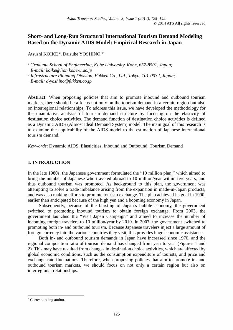
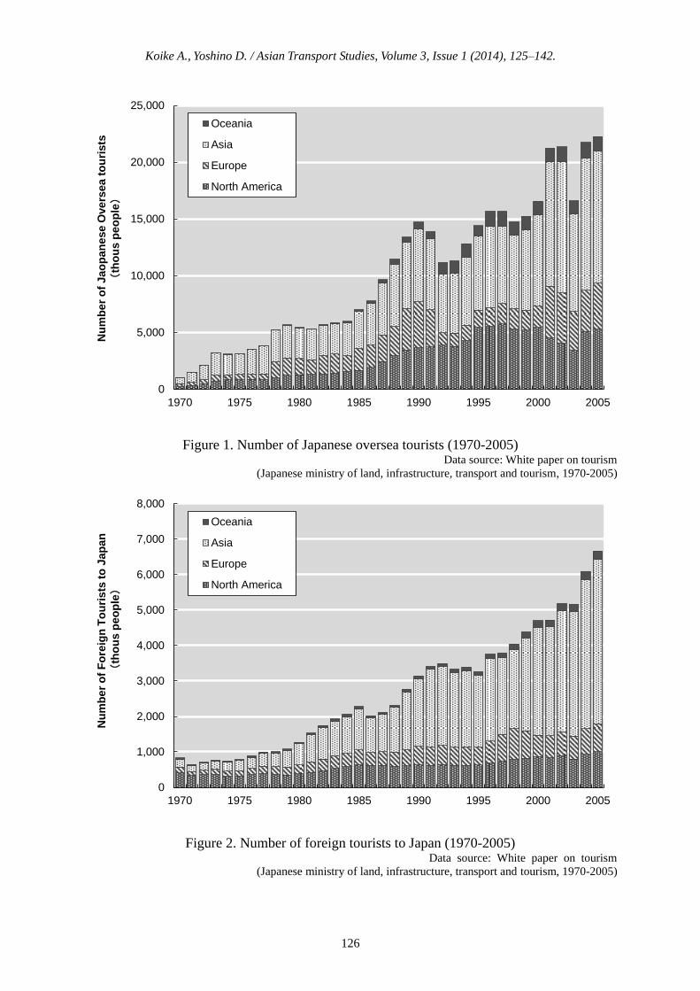
Both in- and outbound tourism demands in Japan have increased since 1970, and the

regional composition ratio of tourism demand has changed from year to year (Figures 1 and

2). This may have resulted from changes in destination choice activities, which are affected by

global economic conditions, such as the consumption expenditure of tourists, and price and

exchange rate fluctuations. Therefore, when proposing policies that aim to promote in- and

outbound tourism markets, we should focus on not only a certain region but also on

interregional relationships.

Corresponding author.

Koike A., Yoshino D. / Asian Transport Studies, Volume 3, Issue 1 (2014), 125–142.

126

0

5,000

10,000

15,000

20,000

25,000

1970 1975 1980 1985 1990 1995 2000 2005

Nu

mb

er

of

Jao

pa

ne

se O

vers

ea t

ou

rists

（th

ou

s p

eo

ple）

Oceania

Asia

Europe

North America

Figure 1. Number of Japanese oversea tourists (1970-2005)

Data source: White paper on tourism

(Japanese ministry of land, infrastructure, transport and tourism, 1970-2005)

0

1,000

2,000

3,000

4,000

5,000

6,000

7,000

8,000

1970 1975 1980 1985 1990 1995 2000 2005

Nu

mb

er

of

Fo

reig

n T

ou

rists

to

Jap

an

（th

ou

s p

eo

ple）

Oceania

Asia

Europe

North America

Figure 2. Number of foreign tourists to Japan (1970-2005)

Data source: White paper on tourism

(Japanese ministry of land, infrastructure, transport and tourism, 1970-2005)


127

We have developed the methodology for the quantitative analysis of tourism demand

structure by focusing on the elasticity of destination choice activities. The demand function of

destination choice activities is defined as a Dynamic AIDS (Almost Ideal Demand System)

model. This model was developed to estimate various elasticities such as own-price,

cross-price, and expenditure, and this approach has been applied in the European tourism

market (e.g., Durbarry and Sinclair, 2003). However, no study has investigated the case of

Japan. Therefore, the main goal here is to examine the applicability of the Dynamic AIDS

model to the estimation of Japanese international tourism demand.

This paper is organized as follows. Section 2 reviews the existing literature focusing on

the estimation of tourism demand. In Section 3, the theory and characteristics of the Dynamic

AIDS model proposed in this study are described. Section 4 describes results of the model

estimation; main conclusions and future tasks are summarized in Section 5.

2. LITERATURE REVIEW

2.1 Traditional Approach to Estimating Tourism Demand

Much of the literature on tourism demand has examined demand at the national level,

although it can also be examined for different components of tourism, such as accommodation

or attractions. It is known that tourism demand is responsive to variables such as income,

relative prices, and exchange rate. What is not known is how the responsiveness of demand to

changes in these variables alters during a region’s economic transition and integration into the

wider international community. Furthermore, the degrees of complementarity and

substitutability between destinations and the extent to which these change during periods of

economic transition need to be examined.

A number of models have been used in the literature to estimate tourism demand. The

large majority of studies of tourism demand have been based on single equation models of

demand, estimated within a static theory. This kind of model is not derived from consumer

demand theory, and it cannot quantify the changes in demand behavior that occur over time.

Subsequently, innovations in methodology were introduced in the form of single

equation models of demand estimated using an error correction methodology (e.g., Loeb,

1982; Uysal and Crompton, 1984). Further, Song et al. (2000) used the error correction model

to estimate UK tourism demand in the form of visits per capita to outbound destinations and

demonstrated that the model has good estimation ability.

This modeling approach has the advantage of explicit treatment of the time dimension

of tourism demand behavior, and allows for improved econometric estimation of the specified

equations. However, as Durbarry and Sinclair (2003) noted, the main problem of the

traditional single equation model concerns the lack of reliability in the accuracy of the

provided results, because the approach lacks a strict basis in consumer demand theory. The

AIDS model of tourism demand is clearly superior in this respect.

2.2 The AIDS Model

A further approach to tourism demand estimation involves a system of equation models such

as the AIDS model. The AIDS model is used in the field of household expenditure analysis,

consumption of goods, trade shares, etc. (e.g., Blundell and Browning, 1994; Eakin and

Gallagher, 2003; Choo et al., 2007). The advantages of the model relate to its strict grounding

in economic theory, the relative simplicity with which it can be estimated, and the flexibility


128

with which it can be applied to different contexts.

Recent applications in the field of tourism suggest that Deaton and Muellbauer’s (1980)

AIDS model provides a well-structured framework for modeling tourism demand: it is based

on economic theory, it satisfies the principle of choice exactly, and can be used to test

homogeneity and symmetry restrictions. Some studies have applied this approach in current

tourism demand analysis (e.g., Mello et al., 2002; Witt and Witt, 1995; Durbarry, 2002). Until

recently, the literature on AIDS has been focused on the static solution. The static AIDS

model assumes that there is no difference between short- and long-run behaviors, which

means that consumers’ behavior is always in equilibrium. However, it is the case that many

factors often cause consumers to be out of equilibrium until full adjustment takes place.

Therefore, the assumption of the static AIDS model is unrealistic in some cases.

As a result of the inability of the long-run specification to explain dynamic adjustment

of tourism demand, some researchers have recently focused on not only long-run solutions but

also on short-run dynamics by using the Dynamic AIDS model (e.g., Durbarry and Sinclair,

2003; Li et al., 2010; Chang et al., 2012). For example, Durbarry and Sinclair (2003) examine

the magnitudes and determinants of changes in destination shares of a major tourist origin

market based on the dynamic AIDS model. They used the model to quantify the

responsiveness of French tourism demand in European countries to changes in price index,

and both long- and short-run demand elasticities were calculated. Li et al. (2010) and Chang

et al. (2012) also estimated the price competitiveness and interdependencies of tourism

demand for competing destinations in both long- and short-run error correction specifications.

However, there are few empirical studies of international tourism demand using

econometric models for Japan. As previous estimates from AIDS models in the literature have

suggested that useful implications can be drawn regarding tourism competitiveness, the AIDS

approach for both static and dynamic specifications is used here to investigate the Japanese

in- and outbound demand for various destinations/origins worldwide.

3. MODEL EXPLANATION AND DATA

3.1 Traditional Static AIDS Model

In this section, the theory and characteristics of the Dynamic AIDS model proposed in this

study are described. First, we introduce the traditional static AIDS model that forms the basis

of the Dynamic AIDS model.

Following Deaton and Muellbauer (1980), we define the tourism expenditure function

of i-th destination region as:

i ii j jiiji ii

ipupppupE

00 lnln2

1ln;ln (1)

where,

E : total of tourists’ expenditure,

p : price of tourism,

u : utility,

i : destination region,

j : alternative destinations,

0 , i , 0 , i ,

ij : parameters that need to be estimated.


129

The demand functions can be derived directly from equation (1). It is a fundamental

property of the cost function (see Shephard, 1970) that its price derivatives are the quantities

demanded: ii qpupE ; ; we find the budget share of i-th destination region wi as

follows.

ii

iiii

p

upE

p

upE

upE

p

upE

qpw

ln

;ln;

;;

(2)

Hence, logarithmic differentiation of (1) gives the budget shares as a function of prices

and utility:

i iij jijii

ipupw

0ln (3)

where the limitation jiij is imposed.

For a utility-maximizing consumer, total expenditure x is equal to E(p;u) and this

equality can be inverted to give u as a function of p and x, the indirect utility function. If we

do this for (1) and substitute the result into (3), we have the budget shares as a function of p

and x; these are the AIDS demand functions in budget share form:

P

xpw ij jijii lnln (4)

where P is price index and is expressed as follows.

　　 i j jiiji ii ppp lnln

2

1lnln 0 P (5)

The restrictions on the parameters comply with the assumptions and ensure that

equation (5) defines P as a linear homogeneous function of individual prices. If prices are

relatively collinear, P will be approximately proportional to any approximately defined price

index, for example, the one used by Deaton and Muellbauer (1980). Hence, in this study, P in

equation (5) can be simplified using the Stone price index (Stone, 1954).

　　　　　 i ii indexpriceStonepw )(lnln P (6)

3.2 Formulation of the Dynamic AIDS Model

A static AIDS specification ignores potential significant short-run elasticity measures that

differ from the long-run estimates. Moreover, in the context of tax policy and business

strategy, decision makers are more likely to be concerned with short-run elasticity estimates

and the speed at which these estimates reach their long-run level. A dynamic AIDS model that

incorporates such short-run estimates is an error correction representation of the AIDS model.

This form is described as the partial differential equation of the first order. In this next

equation, L means long run and S means short-run:


130

　　1

1111 lnlnlnlnt

L

itjt

L

qitj

L

itit

t

S

ijt

S

itj

S

ititP

xpw

P

xpw (7)

where,

: the difference operator (1

ttt

xxx ).

This equation captures the dynamics of tourism demand, showing that current changes

in budget shares depend on not only current change in the normal AIDS explanatory variables

but also on the extent of consumer disequilibrium in the previous period. In the long run, the

coefficients of the price variables, ij , represent the absolute change in the price of region j,

ceteris paribus. Thus, the price variables take account of the effective price in the destination

region i relative to that in other destinations. The i coefficients represent the absolute

change in the i-th expenditure share given a 1% change in real per capita expenditure. The

parameter measures the speed of adjustment to the long-run equilibrium, for example,

=1 adjustment is instantaneous.

The restrictions on the parameters of (1) imply restrictions on the parameters of the

AIDS equation (7). We take these in three sets.

Adding-up restrictions:

　 i i

term

ij

term

ii

term

i SLterm ,0,0,1 (8)

Homogeneity:

SLtermj

term

ij ,0 　 (9)

Symmetry:

SLtermterm

ji

term

ij , 　　 (10)

Provided (8), (9), and (10) hold, equation (7) represents a system of demand functions

that add up to total expenditure ( 1i iw ), that are homogeneous of degree zero in prices

and total expenditure taken together, and that satisfy Slutsky symmetry. There are many

constraint conditions in the Dynamic AIDS model. In such cases, the SURE estimation

method is often used as a parameter estimation method (Zellner, 1962). Therefore, this

method is also used in this study.

If these three restrictions are satisfied, expenditure and price elasticities cannot be

directly accessed in (7), given its linear-log form. Nevertheless, the elasticities can be

retrieved from coefficients in (7) by means of:

Expenditure elasticity:

i

term

iterm

iw

1 (11)

Own-price elasticity:

1term

i

i

term

iiterm

iiw

(12)


131

Cross-price elasticity:

i

jterm

i

i

term

ijterm

ijw

w

w

(13)

where,

wi : the sample’s average share of destination i in the base year,

wj : the sample’s average share of destination j in the base year.

3.3 Data

3.3.1 Outbound tourism demand

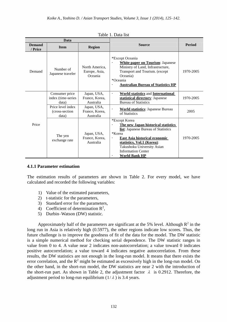
The data used in the outbound tourism analysis are shown in Table 1. The number of Japanese

travelers for each region is indicated as a demand variable. It is assumed that three price

variables affect the demand of Japanese outbound tourism: the tourism expenditure of

Japanese overseas tourists, the price of commodities in each region, and the exchange rate.

The panel data of commodity prices are calculated from the consumer price index (time-series

data) and the price level index (cross-sectional data) for 1970–2005 because of data

availability. Price data are not organized by regional level; thus, the regional data are replaced

by a representative country (i.e., North America: USA; Europe: France; Asia: Korea; and

Oceania: Australia). In addition, transportation costs are excluded from the price index in this

study for the following reasons. First, changes of transportation costs are included in changes

of commodity price, and relatively speaking, the proportion of transport cost to total

expenditure is stable. For example, the rise in gasoline price affects global markets; therefore,

the relative gasoline price remains unchanged. Second, transport data are not available from

each country’s statistics. In fact, in some studies, transportation costs had been excluded from

the price index (e.g., Durbarry and Sinclair, 2003)

3.3.2 Inbound tourism demand

The relative price data are common to both the inbound and outbound analyses. Only the

tourism demand data in the inbound analysis are different from the outbound study; the

number of foreign tourists to Japan (see Japanese ministry of land, infrastructure, transport

and tourism, 1970-2005) indicates inbound demand.

Because of model characteristics, however, we should note that the inbound analysis

based on the AIDS model has two technical problems. First, although this model should

ideally deal with four consumers (i.e., North America, Europe, Asia, and Oceania), the AIDS

model assumes only one consumer, and thus there is a theoretical mismatch. Second, for the

inbound case, the AIDS model cannot consider relative prices (except Japan) because this

model determines only one demand (i.e., tourism demand to Japan). These two issues

obviously need to be addressed. However, in the present trial implementation, these issues

remain in our analysis. Directions for future research are discussed in Section 5.2.

4. EMPIRICAL RESULTS

4.1 Results of Outbound Tourism Demand


132

Table 1. Data list

Data

Source Period Demand

/ Price Item Region

Demand Number of

Japanese traveler

North America,

Europe, Asia,

Oceania

*Except Oceania

White paper on Tourism: Japanese

Ministry of Land, Infrastructure,

Transport and Tourism. (except

Oceania)

*Oceania

Australian Bureau of Statistics HP

1970-2005

Price

Consumer price

index (time-series

data)

Japan, USA,

France, Korea,

Australia

World statistics and International

statistical directory: Japanese

Bureau of Statistics

1970-2005

Price level index

(cross-section

data)

Japan, USA,

France, Korea,

Australia

World statistics: Japanese Bureau

of Statistics 2005

The yen

exchange rate

Japan, USA,

France, Korea,

Australia

*Except Korea

The new Japan historical statistics

list: Japanese Bureau of Statistics

*Korea

East Asia historical economic

statistics, Vol.1 (Korea):

Takushoku University Asian

Information Center

World Bank HP

1970-2005

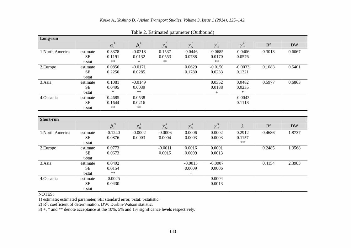
4.1.1 Parameter estimation

The estimation results of parameters are shown in Table 2. For every model, we have

calculated and recorded the following variables:

1) Value of the estimated parameters,

2) t-statistic for the parameters,

3) Standard error for the parameters,

4) Coefficient of determination R2,

5) Durbin–Watson (DW) statistic.

Approximately half of the parameters are significant at the 5% level. Although R2 in the

long run in Asia is relatively high (0.5977), the other regions indicate low scores. Thus, the

future challenge is to improve the goodness of fit of the data for the model. The DW statistic

is a simple numerical method for checking serial dependence. The DW statistic ranges in

value from 0 to 4. A value near 2 indicates non-autocorrelation; a value toward 0 indicates

positive autocorrelation; a value toward 4 indicates negative autocorrelation. From these

results, the DW statistics are not enough in the long-run model. It means that there exists the

error correlation, and the R2 might be estimated as excessively high in the long-run model. On

the other hand, in the short-run model, the DW statistics are near 2 with the introduction of

the short-run part. As shown in Table 2, the adjustment factor is 0.2912. Therefore, the

adjustment period to long-run equilibrium ( /1 ) is 3.4 years.


133

Table 2. Estimated parameter (Outbound)

Long-run

L

i L

i L

i1 L

i2 L

i3 L

i4 R2 DW

1.North America estimate 0.3378 -0.0218 0.1537 -0.0446 -0.0685 -0.0406 0.3013 0.6067

SE 0.1191 0.0132 0.0553 0.0788 0.0170 0.0576

t-stat ** + **

**

2.Europe estimate 0.0856 -0.0171 0.0629 -0.0150 -0.0033 0.1083 0.5401

SE 0.2250 0.0285 0.1780 0.0233 0.1321

t-stat

3.Asia estimate 0.1081 -0.0149 0.0352 0.0482 0.5977 0.6863

SE 0.0495 0.0039 0.0188 0.0235

t-stat * ** + *

4.Oceania estimate 0.4685 0.0538 -0.0043

SE 0.1644 0.0216 0.1118

t-stat ** **

Short-run

S

i S

i1 S

i2 S

i3 S

i4 R2 DW

1.North America estimate -0.1240 -0.0002 -0.0006 0.0006 0.0002 0.2912 0.4686 1.8737

SE 0.0876 0.0003 0.0004 0.0003 0.0003 0.1157

t-stat **

2.Europe estimate 0.0773 -0.0011 0.0016 0.0001 0.2485 1.3568

SE 0.0673 0.0015 0.0009 0.0013

t-stat +

3.Asia estimate 0.0492 -0.0015 -0.0007 0.4154 2.3983

SE 0.0154 0.0009 0.0006

t-stat ** +

4.Oceania estimate -0.0025 0.0004

SE 0.0430 0.0013

t-stat

NOTES:

1) estimate: estimated parameter, SE: standard error, t-stat: t-statistic.

2) R2: coefficient of determination, DW: Durbin-Watson statistic. 3) +, * and ** denote acceptance at the 10%, 5% and 1% significance levels respectively.


134

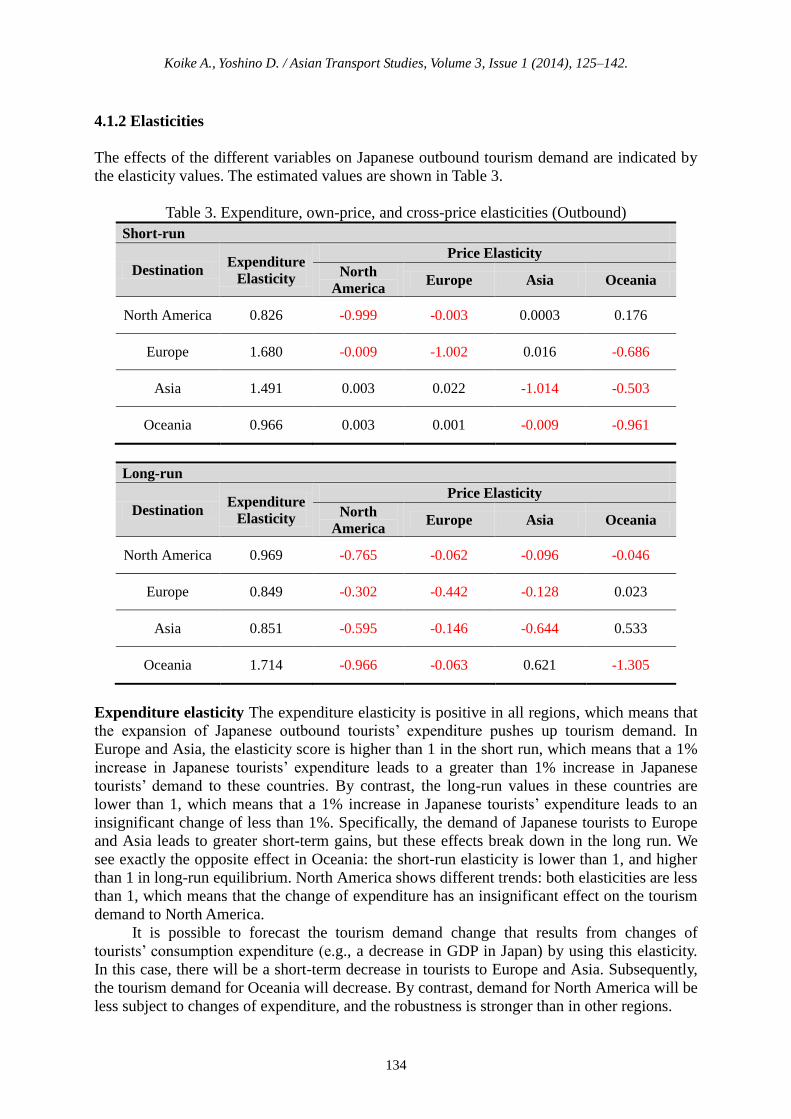
4.1.2 Elasticities

The effects of the different variables on Japanese outbound tourism demand are indicated by

the elasticity values. The estimated values are shown in Table 3.

Table 3. Expenditure, own-price, and cross-price elasticities (Outbound)

Short-run

Destination Expenditure

Elasticity

Price Elasticity

North

America Europe Asia Oceania

North America 0.826 -0.999 -0.003 0.0003 0.176

Europe 1.680 -0.009 -1.002 0.016 -0.686

Asia 1.491 0.003 0.022 -1.014 -0.503

Oceania 0.966 0.003 0.001 -0.009 -0.961

Long-run

Destination Expenditure

Elasticity

Price Elasticity

North


North America 0.969 -0.765 -0.062 -0.096 -0.046

Europe 0.849 -0.302 -0.442 -0.128 0.023

Asia 0.851 -0.595 -0.146 -0.644 0.533

Oceania 1.714 -0.966 -0.063 0.621 -1.305

Expenditure elasticity The expenditure elasticity is positive in all regions, which means that

the expansion of Japanese outbound tourists’ expenditure pushes up tourism demand. In

Europe and Asia, the elasticity score is higher than 1 in the short run, which means that a 1%

increase in Japanese tourists’ expenditure leads to a greater than 1% increase in Japanese

tourists’ demand to these countries. By contrast, the long-run values in these countries are

lower than 1, which means that a 1% increase in Japanese tourists’ expenditure leads to an

insignificant change of less than 1%. Specifically, the demand of Japanese tourists to Europe

and Asia leads to greater short-term gains, but these effects break down in the long run. We

see exactly the opposite effect in Oceania: the short-run elasticity is lower than 1, and higher

than 1 in long-run equilibrium. North America shows different trends: both elasticities are less

than 1, which means that the change of expenditure has an insignificant effect on the tourism

demand to North America.

It is possible to forecast the tourism demand change that results from changes of

tourists’ consumption expenditure (e.g., a decrease in GDP in Japan) by using this elasticity.

In this case, there will be a short-term decrease in tourists to Europe and Asia. Subsequently,

the tourism demand for Oceania will decrease. By contrast, demand for North America will be

less subject to changes of expenditure, and the robustness is stronger than in other regions.


135

Own-price elasticity The own-price elasticity (the diagonal values in Table 3) is negative in

all regions, which means that the increase of prices and exchange rate with Japan will

decrease demand from Japanese tourists. The interpretation of the elasticity is the same with

expenditure. For example, a 1% increase in relative prices of Europe results in a decrease of

1.002% in Japanese short-term demand for tourism. However, in the long run, the rate of

decrease will rebound to 0.442%. Asia indicates the same trend as Europe. Oceania shows

exactly different trends with Europe and Asia. North America is less subject to changing of

their own-price.

Because of the influence of the high yen, the number of Japanese who travel abroad

recently has been increasing. Consequently, although price changes will have a greater impact

on short-run demand for Europe and Asia, this impact will decrease in the long run.

Cross-price elasticity The own-price elasticity values are high relative to those of the

cross-price elasticity (the off-diagonal values in Table 3). These values indicate the sensitivity

of demand for each destination to an increase in price relative to those of its competitors. For

example, in the long run, the results indicate that a 1% increase in price in Oceania results in a

decrease of 0.966% in Japanese demand for North America, an insignificant change in

demand for Europe, and an increase of 0.621% in demand for Asia.

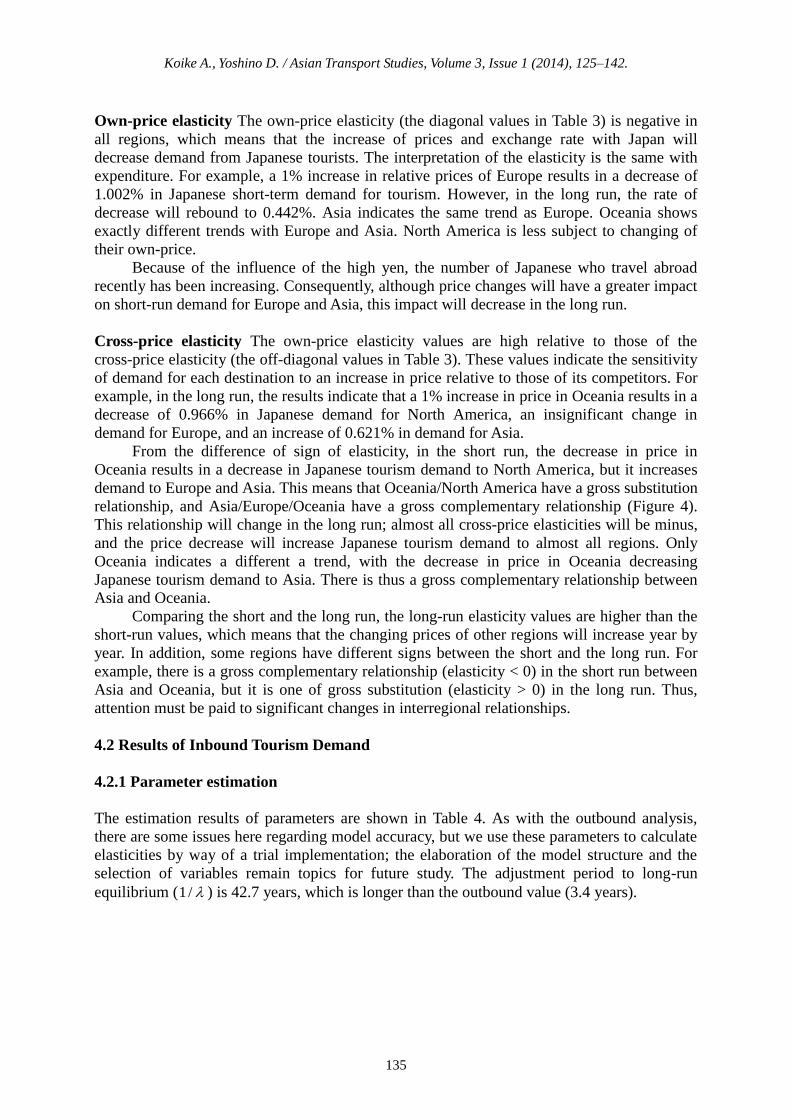
From the difference of sign of elasticity, in the short run, the decrease in price in

Oceania results in a decrease in Japanese tourism demand to North America, but it increases

demand to Europe and Asia. This means that Oceania/North America have a gross substitution

relationship, and Asia/Europe/Oceania have a gross complementary relationship (Figure 4).

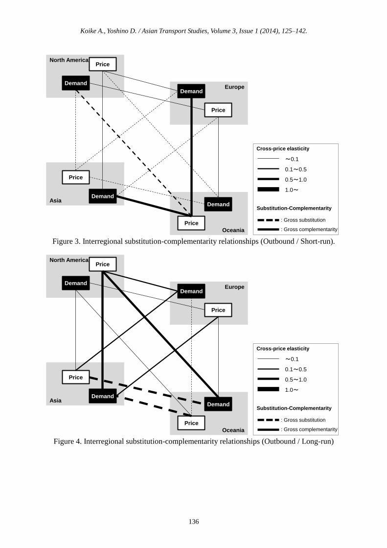
This relationship will change in the long run; almost all cross-price elasticities will be minus,

and the price decrease will increase Japanese tourism demand to almost all regions. Only

Oceania indicates a different a trend, with the decrease in price in Oceania decreasing

Japanese tourism demand to Asia. There is thus a gross complementary relationship between

Asia and Oceania.

Comparing the short and the long run, the long-run elasticity values are higher than the

short-run values, which means that the changing prices of other regions will increase year by

year. In addition, some regions have different signs between the short and the long run. For

example, there is a gross complementary relationship (elasticity < 0) in the short run between

Asia and Oceania, but it is one of gross substitution (elasticity > 0) in the long run. Thus,

attention must be paid to significant changes in interregional relationships.

4.2 Results of Inbound Tourism Demand

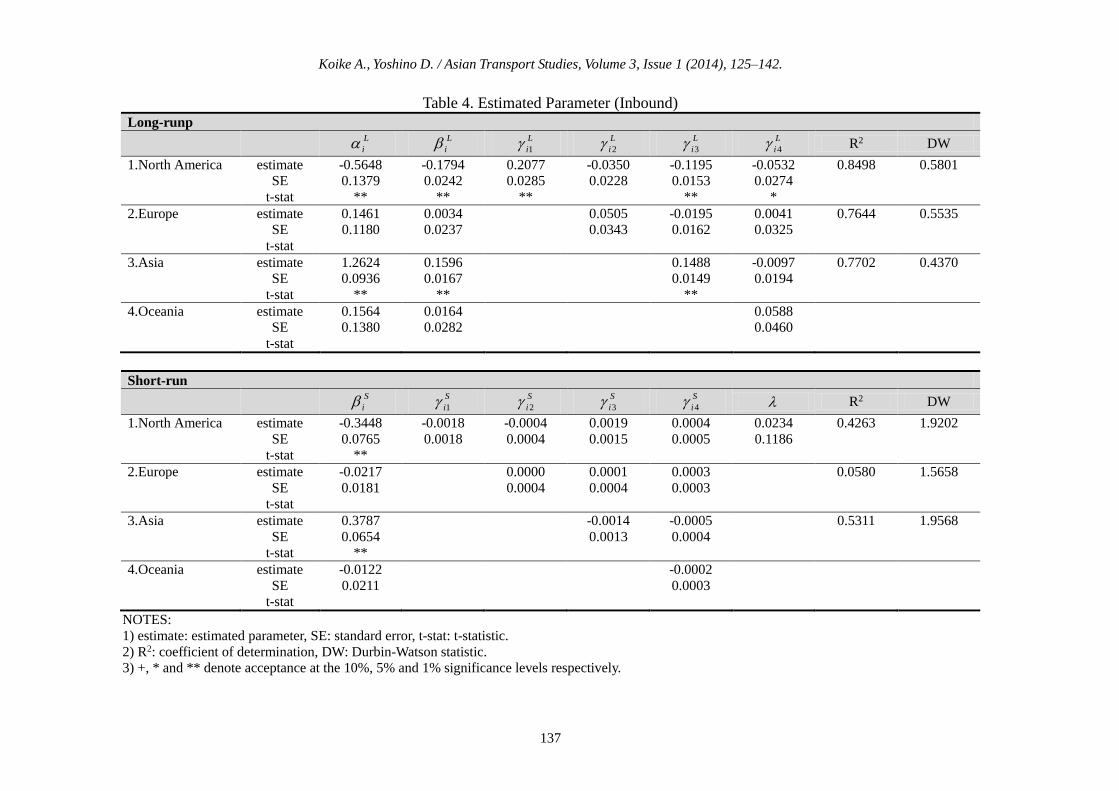
4.2.1 Parameter estimation

The estimation results of parameters are shown in Table 4. As with the outbound analysis,

there are some issues here regarding model accuracy, but we use these parameters to calculate

elasticities by way of a trial implementation; the elaboration of the model structure and the

selection of variables remain topics for future study. The adjustment period to long-run

equilibrium ( /1 ) is 42.7 years, which is longer than the outbound value (3.4 years).


136

Oceania

Europe

Asia

North America

Demand

Price

Demand

Price

Demand

Price

Demand

Price

～0.1

0.1～0.5

0.5～1.0

1.0～

Cross-price elasticity

: Gross substitution

: Gross complementarity

Substitution-Complementarity

Figure 3. Interregional substitution-complementarity relationships (Outbound / Short-run).

Oceania

Europe

Asia

North America

Demand

Price

Demand

Price

Demand

Price

Demand

Price

～0.1

0.1～0.5

0.5～1.0

1.0～





Figure 4. Interregional substitution-complementarity relationships (Outbound / Long-run)


137

Table 4. Estimated Parameter (Inbound)

Long-runp

L

i L

i L

i1 L

i2 L

i3 L

i4 R2 DW

1.North America estimate -0.5648 -0.1794 0.2077 -0.0350 -0.1195 -0.0532 0.8498 0.5801

SE 0.1379 0.0242 0.0285 0.0228 0.0153 0.0274

t-stat ** ** ** ** *

2.Europe estimate 0.1461 0.0034 0.0505 -0.0195 0.0041 0.7644 0.5535

SE 0.1180 0.0237 0.0343 0.0162 0.0325

t-stat

3.Asia estimate 1.2624 0.1596 0.1488 -0.0097 0.7702 0.4370

SE 0.0936 0.0167 0.0149 0.0194

t-stat ** ** **

4.Oceania estimate 0.1564 0.0164 0.0588

SE 0.1380 0.0282 0.0460

t-stat

Short-run

S

i S

i1 S

i2 S

i3 S

i4 R2 DW

1.North America estimate -0.3448 -0.0018 -0.0004 0.0019 0.0004 0.0234 0.4263 1.9202

SE 0.0765 0.0018 0.0004 0.0015 0.0005 0.1186

t-stat **

2.Europe estimate -0.0217 0.0000 0.0001 0.0003 0.0580 1.5658

SE 0.0181 0.0004 0.0004 0.0003

t-stat

3.Asia estimate 0.3787 -0.0014 -0.0005 0.5311 1.9568

SE 0.0654 0.0013 0.0004

t-stat **

4.Oceania estimate -0.0122 -0.0002

SE 0.0211 0.0003

t-stat

NOTES:

1) estimate: estimated parameter, SE: standard error, t-stat: t-statistic.

2) R2: coefficient of determination, DW: Durbin-Watson statistic. 3) +, * and ** denote acceptance at the 10%, 5% and 1% significance levels respectively.


138

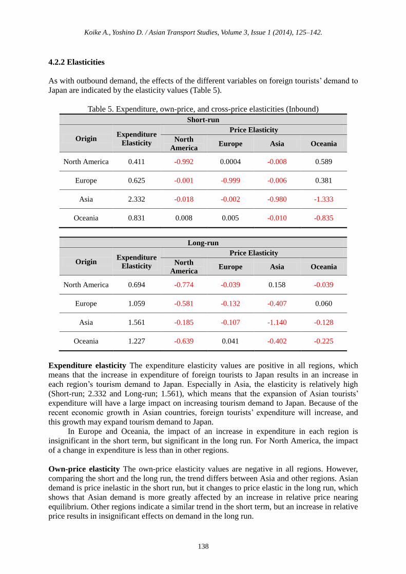
4.2.2 Elasticities

As with outbound demand, the effects of the different variables on foreign tourists’ demand to

Japan are indicated by the elasticity values (Table 5).

Table 5. Expenditure, own-price, and cross-price elasticities (Inbound)

Short-run

Origin Expenditure

Elasticity

Price Elasticity

North


North America 0.411 -0.992 0.0004 -0.008 0.589

Europe 0.625 -0.001 -0.999 -0.006 0.381

Asia 2.332 -0.018 -0.002 -0.980 -1.333

Oceania 0.831 0.008 0.005 -0.010 -0.835

Long-run

Origin Expenditure

Elasticity

Price Elasticity

North


North America 0.694 -0.774 -0.039 0.158 -0.039

Europe 1.059 -0.581 -0.132 -0.407 0.060

Asia 1.561 -0.185 -0.107 -1.140 -0.128

Oceania 1.227 -0.639 0.041 -0.402 -0.225

Expenditure elasticity The expenditure elasticity values are positive in all regions, which

means that the increase in expenditure of foreign tourists to Japan results in an increase in

each region’s tourism demand to Japan. Especially in Asia, the elasticity is relatively high

(Short-run; 2.332 and Long-run; 1.561), which means that the expansion of Asian tourists’

expenditure will have a large impact on increasing tourism demand to Japan. Because of the

recent economic growth in Asian countries, foreign tourists’ expenditure will increase, and

this growth may expand tourism demand to Japan.

In Europe and Oceania, the impact of an increase in expenditure in each region is

insignificant in the short term, but significant in the long run. For North America, the impact

of a change in expenditure is less than in other regions.

Own-price elasticity The own-price elasticity values are negative in all regions. However,

comparing the short and the long run, the trend differs between Asia and other regions. Asian

demand is price inelastic in the short run, but it changes to price elastic in the long run, which

shows that Asian demand is more greatly affected by an increase in relative price nearing

equilibrium. Other regions indicate a similar trend in the short term, but an increase in relative

price results in insignificant effects on demand in the long run.


139

For example, if the trend of the high yen continues in the future, travel demand to Japan

is unlikely to vary by region in the short run; however, demand from Asian tourists may

decrease in the long run.

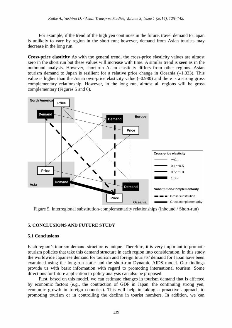
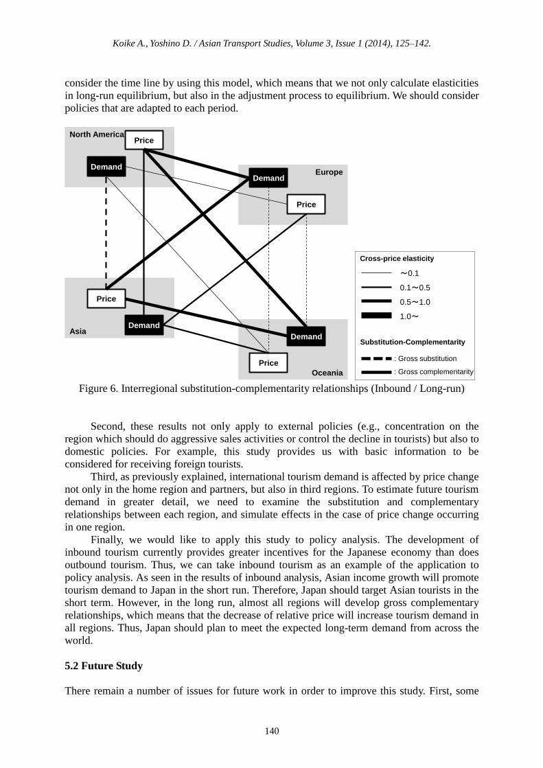
Cross-price elasticity As with the general trend, the cross-price elasticity values are almost

zero in the short run but these values will increase with time. A similar trend is seen as in the

outbound analysis. However, short-run Asian elasticity differs from other regions. Asian

tourism demand to Japan is resilient for a relative price change in Oceania (–1.333). This

value is higher than the Asian own-price elasticity value (–0.980) and there is a strong gross

complementary relationship. However, in the long run, almost all regions will be gross

complementary (Figures 5 and 6).

Oceania

Europe

Asia

North America

Demand

Price

Demand

Price

Demand

Price

Demand

Price

～0.1

0.1～0.5

0.5～1.0

1.0～





Figure 5. Interregional substitution-complementarity relationships (Inbound / Short-run)

5. CONCLUSIONS AND FUTURE STUDY

5.1 Conclusions

Each region’s tourism demand structure is unique. Therefore, it is very important to promote

tourism policies that take this demand structure in each region into consideration. In this study,

the worldwide Japanese demand for tourism and foreign tourists’ demand for Japan have been

examined using the long-run static and the short-run Dynamic AIDS model. Our findings

provide us with basic information with regard to promoting international tourism. Some

directions for future application to policy analysis can also be proposed.

First, based on this model, we can estimate changes in tourism demand that is affected

by economic factors (e.g., the contraction of GDP in Japan, the continuing strong yen,

economic growth in foreign countries). This will help in taking a proactive approach to

promoting tourism or in controlling the decline in tourist numbers. In addition, we can


140

consider the time line by using this model, which means that we not only calculate elasticities

in long-run equilibrium, but also in the adjustment process to equilibrium. We should consider

policies that are adapted to each period.

Oceania

Europe

Asia

North America

Demand

Price

Demand

Price

Demand

Price

Demand

Price

～0.1

0.1～0.5

0.5～1.0

1.0～





Figure 6. Interregional substitution-complementarity relationships (Inbound / Long-run)

Second, these results not only apply to external policies (e.g., concentration on the

region which should do aggressive sales activities or control the decline in tourists) but also to

domestic policies. For example, this study provides us with basic information to be

considered for receiving foreign tourists.

Third, as previously explained, international tourism demand is affected by price change

not only in the home region and partners, but also in third regions. To estimate future tourism

demand in greater detail, we need to examine the substitution and complementary

relationships between each region, and simulate effects in the case of price change occurring

in one region.

Finally, we would like to apply this study to policy analysis. The development of

inbound tourism currently provides greater incentives for the Japanese economy than does

outbound tourism. Thus, we can take inbound tourism as an example of the application to

policy analysis. As seen in the results of inbound analysis, Asian income growth will promote

tourism demand to Japan in the short run. Therefore, Japan should target Asian tourists in the

short term. However, in the long run, almost all regions will develop gross complementary

relationships, which means that the decrease of relative price will increase tourism demand in

all regions. Thus, Japan should plan to meet the expected long-term demand from across the

world.

5.2 Future Study

There remain a number of issues for future work in order to improve this study. First, some


141

model statistics (t-statistics, DW-statistics, and R2) are statistically unwarranted; explanatory

variables should be reviewed.

Second, although the correlation between objective variables and explanatory variables

in the AIDS model was clarified, we do not understand clearly the cause and effect

relationship between these variables. Caution should therefore be applied in the interpretation

of the study findings.

Third, in this study, the world is divided into four regions because of data limitations.

This approach evidently provides a macroscopic viewpoint for analysis of detailed policy

making; thus, future analysis should deal with smaller zones.

In addition, as previously mentioned, there is an inherent problem of consistency with

the inbound analysis in the AIDS model. Because of data availability, we carried out trial

calculations despite this issue, but the model structure should obviously be reviewed in future

study.

Finally, again because of data limitations, the tourism demand structure was estimated

by pooled data, which contained all-purpose overseas trips. However, the demand structure

may be different by region. For example, the price elasticity may be quite different between

sightseeing trips and those for business purposes. We have no data on trip purpose in

outbound tourism. For inbound tourism, such data may be gathered for each region from

immigration statistics, and these data indicate considerable variability across regions,

calculated as a ratio of tourists (sightseeing purpose) to the total number of visitors to Japan:

Asia: 80%, Europe: 61%, North America: 50%, and Oceania: 70%. To elaborate this model,

the disaggregation of trip purpose will be essential.

REFERENCES

Australian Bureau of Statistics (2011). Overseas Arrivals and Departures (www.abs.gov.au/;

Accessed Nov. 1, 2011). (in Japanese)

Blundell, R., Browning, M. (1994). Consumer demand and the life-cycle allocation of

household expenditures. Review of Economic Studies, 61, 57–80.

Chang, C. C., Khamkaew, T., McAleer, M. (2012). Estimating price effects in an almost ideal

demand model of outbound Thai tourism to East Asia. Journal of Tourism Research &

Hospitality, 1 (3). (Online: doi: 10.4172/2324-8807.1000103)

Choo, S., Lee, T., Mokhtarian, P.L. (2007). Do transportation and communications tend to be

substitutes, complements, or neither? – U.S. consumer expenditure perspective, 1984-2002

–. Transportation Research Record, 2010, 121–132.

Deaton, A., Muellbauer, J. (1980). An almost ideal demand system. The American Economic

Review, 70(3), 312–326.

Durbarry, R. (2002). Long Run Structural Tourism Demand Modeling: An Application to

France. Tourism and Travel Research Institute, University of Nottingham, United

Kingdom.

Durbarry, R., Sinclair, M.T. (2003). Market shares analysis -The case of French tourism

demand-. Annals of tourism research, 30(4), 927–941.

Eakins, J.M., Gallagher, L.A. (2003). Dynamic almost ideal demand systems: An empirical

analysis of alcohol expenditure in Ireland. Applied Economics, 35 (9), 1025–1036.

Japanese Ministry of Land, Infrastructure, Transport and Tourism (1970-2005). White paper

on Tourism. (in Japanese)

Japanese Bureau of Immigration (2010). Immigration Statistics (www.moj.go.jp/housei/

toukei/toukei_ichiran_nyukan.html; Accessed Nov. 5, 2010). (in Japanese)


142

Japanese Bureau of Statistics (2011). International Statistical Directory, 1970-1993 (Accessed

Nov. 1, 2011). (in Japanese)

Japanese Bureau of Statistics (2011). World Statistics (www.stat.go.jp/data/sekai/index.htm;

Accessed September 10, 2011). (in Japanese)

Japanese Bureau of Statistics (2006). The New Japan Historical Statistics List. (in Japanese)

Li, G., Song, H., Witt, S. (2010). Modeling tourism demand: A dynamic linear AIDS approach.

Journal of Travel Research, 43(2), 141–150.

Loeb, P.D. (1982). International travel to the United States: an econometric evaluation. Annals

of Tourism Research, 9, 7–20.

Mello, M.D., Pack, A., Sinclair, M. T. (2002). A system of equations model of UK tourism

demand in neighboring countries. Applied Economics, 34, 509–521.

Shephard, R.W. (1970). Theory of Cost and Production Functions. Princeton University Press.

Song, H., Romilly, P., Liu, X. (2000). An empirical study of outbound tourism demand in UK.

Applied Economics, 32, 611–624.

Stone, R. (1954). The Measurement of Consumers’ Expenditure and Behavior in the United

Kingdom, 1920-1938. Volume 1, Cambridge At the University Press.

Takushoku University Asian Information Center (2006). East Asia Historical Economic

Statistics, Vol.1 (Korea), Keiso Shobo. (in Japanese)

Uysal, M., Crompton, J. (1984). Determinants of demand for international tourism flows to

Turkey. Tourism Management, 5, 288–297.

Witt, C., Witt, S. (1995). Forecasting tourism demand: A review of empirical research.

International Journal of Forecasting, 11, 447–475.

World Bank (2011) www.worldbank.org/. Accessed Nov. 1, 2011.

Zellner, A. (1962) An efficient method of estimating seemingly unrelated regressions and tests

for aggregation bias. Journal of the American Statistical Association, 57(298), 348–368.

Date post:	17-Feb-2022
Category:	Documents
Upload:	others
View:	2 times
Download:	0 times

Short-run and Long-run structural international tourism ...

Documents