Short Term Planning and Scheduling For Gasoline Blending ...

Journal Of Petoleum Research & Studies

1st Iraq Oil & Gas Conference (1

ST IOGC) E169

Short Term Planning and Scheduling For Gasoline

Blending in Oil Refineries

Faisal G. Zhqiar*Dr.Prof. Alla-Eldine Hassan**

Dr.Assist Prof. Lamyaa M. Dawood**

*Iraq Oil Ministry: Midland Refineries Company

**UOT Production Engineering and Metallurgy department Iraq. Baghdad.

Abstract

Product blending is an

important optimization task that is

encountered in the operation and

scheduling of important industrial

plants like petroleum refineries. The

key objective of blending is to mix

various intermediate products to

achieve desired properties and

quantities of products with minimum

cost. There are uncertain parameters

which make it very difficult to attain

the optimum allocation of available

resources. Consequently, there is a

need to develop computational

optimization techniques to tackle the

blending issues.

In this research the main objective

is to propose an approach to solve

product blending issue in an optimum

way. The blending problem can be

formulated as an optimization where

its objective is to maximize net profit

while determining the optimal

allocation of intermediate streams to

produce optimum production mix of

final products.

The proposed approach is

introduced for integrating short term

planning and scheduling for product

blending. Two mathematical models

have been proposed. The first model

deals with planning issue for product

blending and the results are regarded

as production guidelines. In the

second scheduling model, scheduling

will treat the production guidelines to

verify optimum allocation for

available resources. The approach

was applied to different real time

case studies form Midland Refineries



ST IOGC) E 170

Company, and the results show the

efficiency and flexibility of this

approach to solve the different case

studies. Also minimize lead time

from 72 to 24 hr in the second case

according to reduction in re-blend

process, in addition to minimize

production cost depending on

optimum allocation for available

resources. The last case study which

is a complicated one, were WIN QSB

version 1.00 software is utilized. The

results gained after 0.031 second

CPU time for planning level and

3.375 second CPU time for

scheduling level. This is considered

as an advantage to the model.

1. Introduction

The petroleum refining

industry is an important kind of

process industries which are vital to

the national economy in any state in

the world [1]. Oil refining is regarded

as the most complex chemical

industries that may involve different

and many complicated processes with

various possible connections.

Challenges facing oil refining

industries are designated as surplus

refining capacity, and the increase in

crude oil prices causing decrease in

profit margins. These challenges are

accompanied by the impact of global

market competition and strict

environmental regulations [2and3]. In

order to compete successfully in

international markets and with global

competition, oil refineries are

increasingly concerned with

improving the planning and

scheduling of their operations to

achieve better economic

performance. Any benefits from

improved control optimization of

processes upstream will be useless if

the final blending step is sub-optimal

[4]. Therefore, optimum recipe for

blended product is considered as a

key question in the refineries, and

become the center of technology

innovations [5]. The short-term

scheduling problem is still one of the

most challenging problems in

operational research due to the

complexity of the scheduling



ST IOGC) E171

operations and the corresponding

process models [1, 6and7].

Product blending and distribution

system scheduling are important parts

of refinery optimisation, because they

are strongly related to ever-changing

market demands and prices. Gasoline

Blending process is generally agreed

as being the most important and

complex problem. Its importance

comes from the fact that gasoline is a

profitable product for refinery where

(60-70%) of a typical refinery's total

revenue comes from the gasoline

sale. On the other hand, the

complexity arises from the large

number of product demands and

quality specifications for each final

product, as well as the limited

number of available resources that

can be used to reach the production

goals [8].Therefore, The goal of

planning and scheduling in refineries

is to maximize the profitability by

choosing the best feed stocks,

operating conditions, and schedules,

while fulfilling product quantity and

quality objectives that are consistent

with marketing commitments[5].

Scheduling of blending process has a

large potential to provide a

competitive benefit for oil refiners

[3]. Significant cost savings and

improved profits can be achieved

through the planning and scheduling

optimization of refinery operations

[1].

2. Problem Definition

At the planning level, the

effects of changeovers and daily

inventories are neglected, and

according to the uncertainty in these

parameters, the determined solution

at the planning level will be

optimistic estimates that cannot be

realized [5]. At the scheduling level

the schedule may be infeasible or

even if it was feasible schedule,

increasing the production cost may

occur according to quantity and

quality giveaway of the blended

product that will be the cause of

increase in lead time and product



ST IOGC) E 172

cost, consequently, the optimality of

the planning solution cannot be

ensured [7]. Therefore, developing

methodology that can effectively

short term production planning and

scheduling in petroleum refineries is

needed to verify the optimality.

The aim of this research is to

develop a framework for short term

planning and scheduling in petroleum

refineries, by using mathematical

model and sensitivity analysis to

predict uncertain parameters. This

framework consists of two levels.

The planning level is the first, in

which Linear Programming model

(LP) or Linear Goal Programming if

there are multi objectives (LGP)

model are proposed. While the

second level MILP model is

proposed for scheduling issue. So the

main objectives of this framework

can be summarized as follows:

Specify the optimum recipe for

each product with minimum cost.

Maximize throughput with

minimum cost.

Specify analysis report for

uncertain parameters.

Minimize lead time.

Maximize utilization of the

equipments and storage tanks.

Minimize operational cost.

Proposed a schedule for the

production plan.

2.1 Production Planning And

Scheduling In Oil Refineries

Production planning is the

discipline related to the high level

decision-making of macro level

problems for allocation of production

capacity. The primary objective of

planning is to determine a feasible

operating plan consisting of

production goals that optimizes a

suitable economic criterion,

maximizing total profit (or

equivalently, of minimizing total

costs), over a specific extended

period of time in the future, typically

in the order of few months to few

years; giving marketing forecasts of



ST IOGC) E173

prices and market demands for

products [9, 10 and 11]. Planning

problems can mainly be distinguished

as strategic, tactical or operational,

based on the decisions involved and

the time horizon considered. The

strategic level planning considers a

time span of more than one year and

covers a whole width of an

organization. At this level,

approximate and/or aggregate models

are adequate and are mainly

considered as future investment

decisions. Tactical level planning

typically involves a midterm horizon

of few months to a year where the

decisions usually include production,

inventory and distribution.

Operational level covers shorter

periods of time spanning from one

week to three months where the

decisions involve actual production

and allocation of resources. For a

general process operations hierarchy,

planning is the highest level of

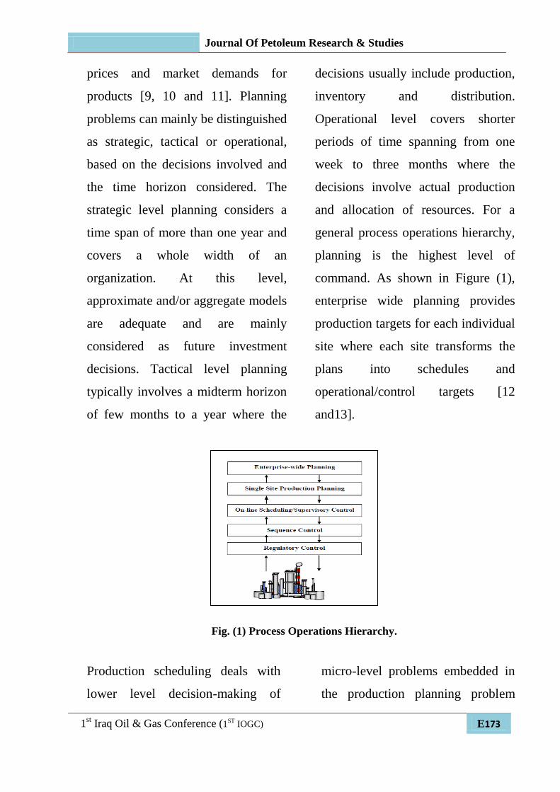
command. As shown in Figure (1),

enterprise wide planning provides

production targets for each individual

site where each site transforms the

plans into schedules and

operational/control targets [12

and13].

Fig. (1) Process Operations Hierarchy.

Production scheduling deals with

lower level decision-making of

micro-level problems embedded in

the production planning problem



ST IOGC) E 174

that involves deciding on the

methodology that determines the

feasible sequence or order and

timing in which various products are

to be produced in each piece of

equipment, so as to meet the

production goals that are laid out by

the planning model. The major

objective of scheduling is to

efficiently utilize the available

equipment among multiple types of

products to be manufactured, to an

extent necessary to satisfy

production goals. Therefore,

optimizing is a suitable economic or

systems performance criterion; over

a short time horizon ranging

typically from several shifts to

several weeks. Scheduling models,

are concerned more with the

feasibility of operations to

accomplish a given number and

order of tasks [8].

The schedule is revised as needed

so that it always starts from what is

actually happening with revisions

that typically occur on each day or on

each shift. Scheduling can be viewed

as a reality check on the planning

process [15]. The main aim of

scheduling is the implementation of

the plan, subjected to the variability

that occurs in the real world. This

variability could be present in the

form of feedstock supplies and

quality, the production process,

customer requirements, or

transportation. Schedulers assess how

production upsets and other changes

will force deviations from the plan.

2.2 The Gasoline Blending Process

The gasoline is one of the

most important refinery products

because it can yield (60 - 70) % of a

typical refinery's total revenue [11,

16 and 17]. Gasoline blending is the

final step of processing gasoline

products. The gasoline blending

operation often determines the

operating conditions of the upstream

units. Due to the importance of the

gasoline blending, a gasoline

blending process is included in the

proposed approach. Gasoline

blending is the process of blending

several gasoline blending stocks that



ST IOGC) E175

are produced in upstream units or

purchased from the market to make

several grades of gasoline according

to the specifications. The objective of

the planning and scheduling for

gasoline blending is to allocate the

available gasoline blending

components in such a way as to meet

product demands and specifications

at the least cost and to produce

products which maximize the overall

profit. Different gasoline blending

stocks have different properties.

Different grades of gasoline also have

different specifications. The core of a

gasoline blending model is the

prediction of gasoline properties from

the properties of the blending stocks.

Some refineries can have up to 30

different gasoline blending feed

stocks [14].

The main blending feed stocks

used are:

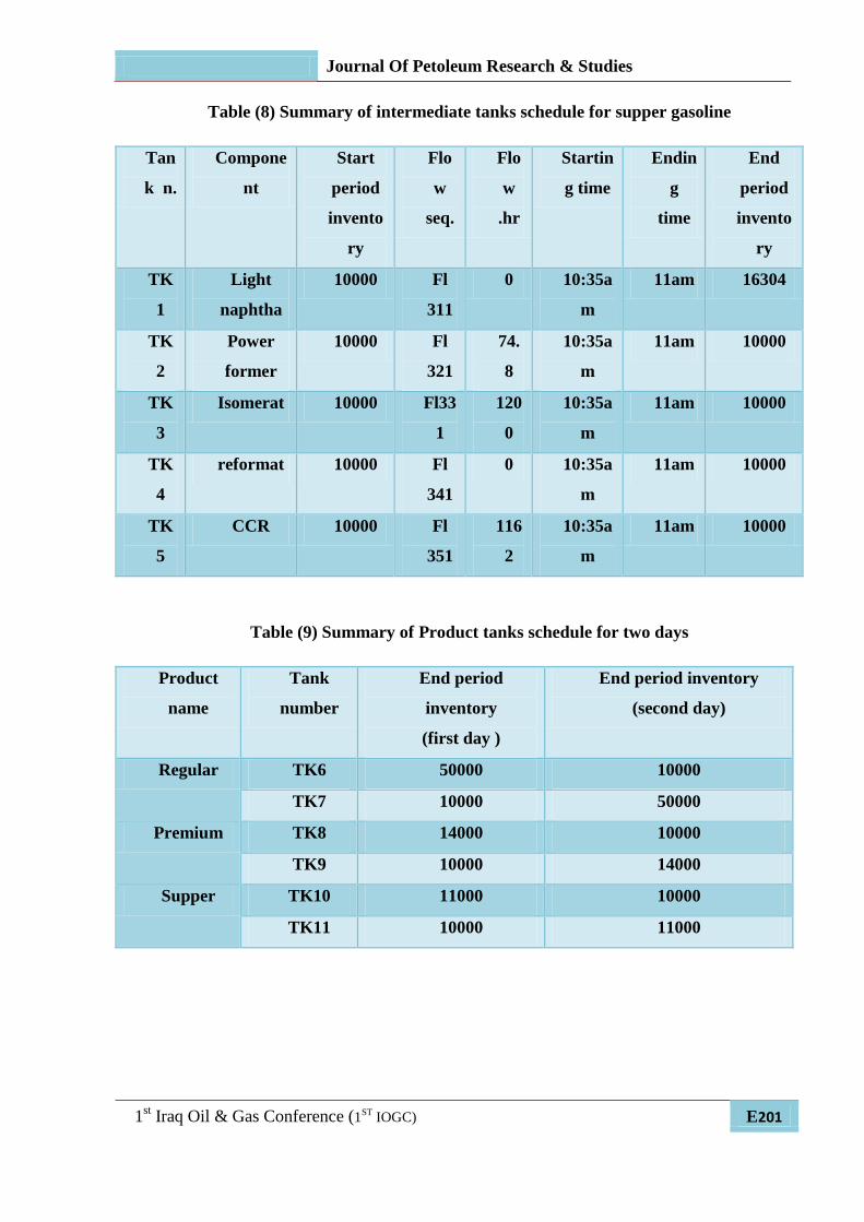
1. Light Straight Run Naphtha or

LSR, which is the gasoline boiling

range cut from the atmospheric

distillation tower.

2. Ismorate the gasoline cut from

isomerization unit.

3. CCR feedstock the gasoline cut

from Continues Catalytic

Regeneration.

4. Reformate1 the gasoline from the

catalytic reforming unit.

5. Reformate2(or power former) from

power former unit

6. Catalytic Cracking gasoline (the

gasoline cut from the Fluidized

Catalytic Cracking Unit

7. Alkylate, the gasoline cut from the

liquid catalyzed alkylation unit.

8. n-Butane, normal butane from

various processing units.

9. 'Hydrocrackate', the gasoline

fraction from the hydrocracker.

10. Additives like Tetra Ethyl Lead

(TEL), Ethanol and Methanol.

The first nine blending stocks are

produced and blended in the

refinery while the additives (TEL,

ethanol and methanol) are

purchased [14 and19]. Therefore,

adjusting the operating conditions of

upstream units according to the

gasoline blending is essential to



ST IOGC) E 176

make the refinery operation

profitable. Gasoline is typically

retailed in grades of regular,

premium and supper, which are

differentiated by the posted octane

number. The octane number (ON)

and Reid Vapor Pressure (RVP) is

the most common required

specifications.

3. Developing Short Term

Planning And Scheduling For

Gasoline Blending

In the present work

integrating short-term planning and

scheduling model for product

blending is proposed, by using

mathematical model and sensitivity

analysis for predication uncertain

parameters.

3.1 Proposed Approach

The proposed approach is

shown in Figure (2). It consists of

two mathematical models with two

levels. The first level deals with the

production planning formulated as

Linear Programming (LP) or Linear

Goal Programming (LGP) if there

are multi objectives to solve the

optimum quantity decision of

products that meet product

specifications with minimum cost.

Then the analyzed results are

incorporated as a fixed decision into

scheduling model (the second

level).The results of the first level

are considered as production

guidelines and utilized as input to

the second level to reduce the

number of variables and

computational results in the

scheduling model. In scheduling

level the main objective is to

implement the production plan with

minimum cost according to due date

and available equipments and

resources.



ST IOGC) E177

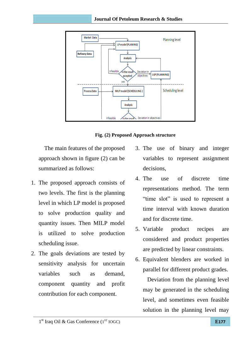
Fig. (2) Proposed Approach structure

The main features of the proposed

approach shown in figure (2) can be

summarized as follows:

1. The proposed approach consists of

two levels. The first is the planning

level in which LP model is proposed

to solve production quality and

quantity issues. Then MILP model

is utilized to solve production

scheduling issue.

2. The goals deviations are tested by

sensitivity analysis for uncertain

variables such as demand,

component quantity and profit

contribution for each component.

3. The use of binary and integer

variables to represent assignment

decisions,

4. The use of discrete time

representations method. The term

“time slot” is used to represent a

time interval with known duration

and for discrete time.

5. Variable product recipes are

considered and product properties

are predicted by linear constraints.

6. Equivalent blenders are worked in

parallel for different product grades.

Deviation from the planning level

may be generated in the scheduling

level, and sometimes even feasible

solution in the planning level may



ST IOGC) E 178

be difficult to apply in the

scheduling level. The deviation

from the planning objectives occurs

because of the following reasons.

1. The effects of change over and daily

inventories are neglected.

2. The uncertainty in demand or

available components specifications.

3. The quality and quantity giveaway

of the intermediate products during

the scheduling horizon because of

the fluctuation in the production

units.

4. In the planning level the product

demands are defined for a period of

time and not for precise delivery

dates.

5. Simultaneous allocation of

equipment cannot be included

within planning level.

As shown in figure (2) the results

are to be analyzed employing

sensitivity analysis. The appropriate

strategy will be according to the

results of the sensitivity analysis

that will be as follow:

1. Optimal solution that will be

accepted.

2. The deviation in goals will be

resolved by linear goal

programming.

3. Infeasible schedule that will be

feedback to the planning level to be

processed.

For the proposed approach it is

assumed that the following are

given:-

(1). Operational planning horizon 7

days.

(2) .Scheduling horizon, 2 days.

(3). A set of component product

tanks with minimum and maximum

capacity restrictions.

(4). A set of blend headers working

in parallel that can be allocated to

each final product.

(5). Initial stocks for components.

(6). Component supplies with known

flow rates from production unit.

(7). Product lifting with constant

flow rates.



ST IOGC) E179

(8). Discrete time representation is

used and the starting time of the

scheduling horizon is (8 AM)

The objectives of planning level are

to determine:

The total volume of each final

product.

The optimum recipes for each

product that minimize cost.

Maximize throughput with

minimum cost.

Specify analysis report for uncertain

parameters.

While the objectives of scheduling

level are to determine:

The optimal timing decisions for

production and storage tasks.

The optimum pumping rates for

components and products.

The assignment of blenders to final

products.

The inventory levels of components

and products in storage tanks.

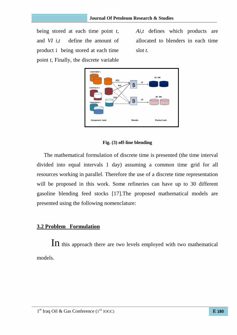
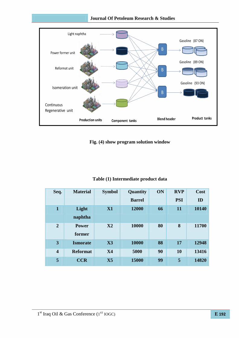
In order to describes the problem

variables, Fig. (3), Illustrates

gasoline blending, which is treated

as two; logistic and quality

problems. Where the logistic defines

the way in which the products are

processed with respect to time and

available equipments and the quality

constraint will explain how the

available components will be

blended or mixed together to

produce on specification products

with minimum cost. The key

decision variables involved in this

problem are the following; The

continuous variable xij defines the

volumetric quantity of component j

that must be transferred to produce

product i during the time slot t

.While yi denotes the volumetric

quantity of product i that may be

blended during each time slot t. The

solution of the scheduling problem

defines the way in which the

products are processed with respect

to time and available equipments.

The continuous variables VJ j,

define the amount of components j



ST IOGC) E 180

being stored at each time point t,

and VI i,t define the amount of

product i being stored at each time

point t, Finally, the discrete variable

Ai,t defines which products are

allocated to blenders in each time

slot t.

Fig. (3) off-line blending

The mathematical formulation of discrete time is presented (the time interval

divided into equal intervals 1 day) assuming a common time grid for all

resources working in parallel. Therefore the use of a discrete time representation

will be proposed in this work. Some refineries can have up to 30 different

gasoline blending feed stocks [17].The proposed mathematical models are

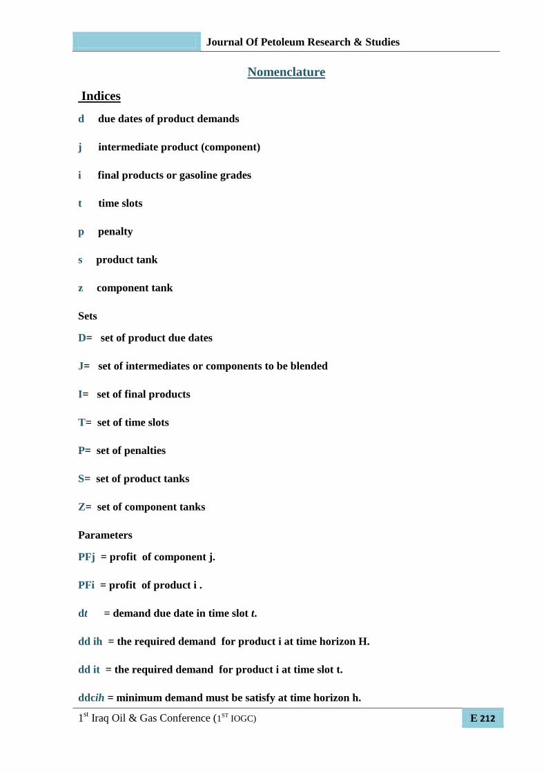
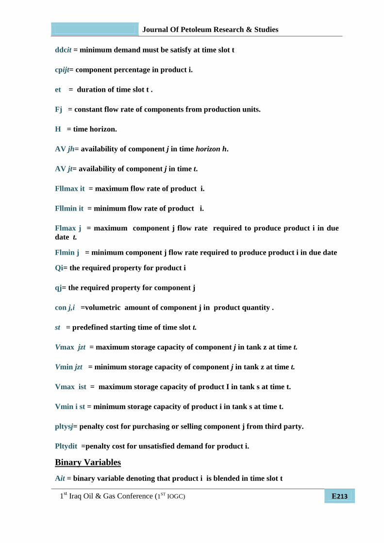
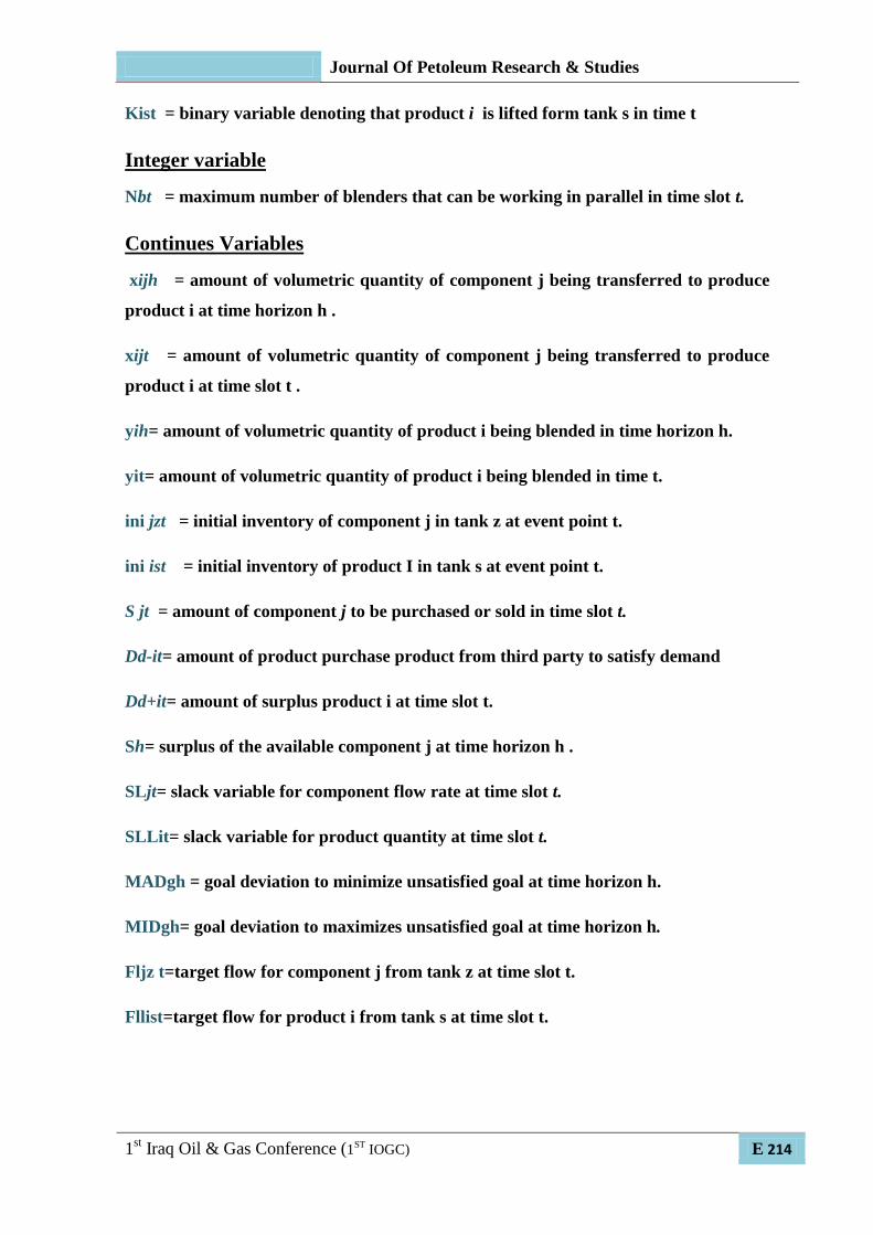
presented using the following nomenclature:

3.2 Problem Formulation

In this approach there are two levels employed with two mathematical

models.



ST IOGC) E181

3.2.1 The Planning Level (Linear Programming)

The first level is the operation planning level. In which

the planning horizon is fixed to one week. The problem is

formulated as LP or if the refinery wanted to verify multi

objectives the model will be formulated as LGP. The goal of

planning level is to determine the optimum quantity decisions.

The main objective in this level is to maximize net profit

subject to meet quality and quantity requirements. The

constraints of this level are formulated as follow.

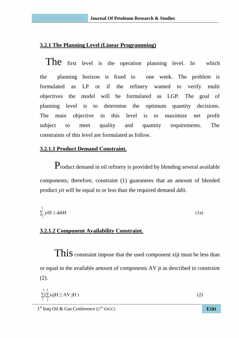
3.2.1.1 Product Demand Constraint.

Product demand in oil refinery is provided by blending several available

components; therefore, constraint (1) guarantees that an amount of blended

product yit will be equal to or less than the required demand ddit.

I

∑ yiH ≤ ddiH (1a) i

3.2.1.2 Component Availability Constraint.

This constraint impose that the used component xijt must be less than

or equal to the available amount of components AV jt as described in constraint

(2).

I J

∑(∑xijH ≤ AV jH ) (2) i j



ST IOGC) E 182

3.2.1.3 Product Quality Constraint.

Every final product specifications reflect the specifications of its

blended components. In this model, Octane Number (ON) and Reid Vapor

Pressure (RVP) are used as the quality index of gasoline and viscosity for fuel

oil; therefore the constraint (3) will satisfy ON requirements and (4) satisfy

RVP requirements.

I J J

∑ ((∑qj xij )-( ∑xij Qi) ≥ 0 ) (3) i j j

I J J

∑ ((∑qj xij )-( ∑xij Qi) ≤ 0 ) (4) i j j

3.2.1.4 Product Composition Constraints

The final product yit will be equal to the summation of its blended

components xijt as expressed below.

I J ∑ ∑xijH = yiH (5) i j

3.2.1.5 Surplus Constraint

Due to the surplus components the penalty constraint may be add to the

objective function and the constraint (6) determines the surplus component Sj

that is equal to the available component AVjH volume – the required volume of

the same component xijt .



ST IOGC) E183

J

SH=∑AVjH - xijH for j=1to J (6) j

Where surplus component Sj is equal to the available component AVjH minus

the required component xijt for mixing of the required product i. Constraint

3.2.1.6 Production Rule Constraints

These constraints include the conditions that describe refinery

limitations like production unit status, inventory situation and managerial

requirements for example if the refinery wanted to contracts to produce specific

quantity for specific product therefore the constraint (1) will be modified to

constraint (7)

I

∑ddciH ≤yiH≤ ddiH (7) i

3.2.1.7 Objective Function.

While satisfying all above constraints, the main objective of the

blending problem is to maximize net profit by maximize contribution profit for

each component pfij Xij – penalty cost pj ) according to availability of

resources the quality and quantity requirement.

I J J

Max ∑ ∑ pfij XijH - ∑ paltys SjH (8a) i j j



ST IOGC) E 184

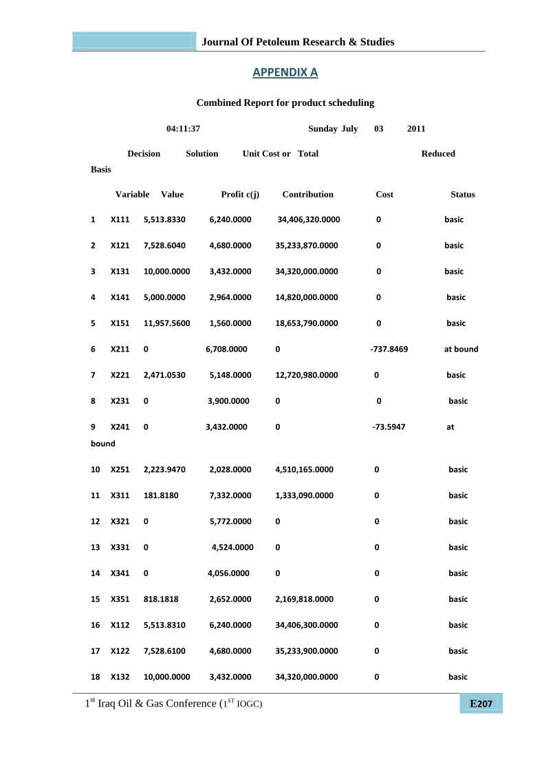
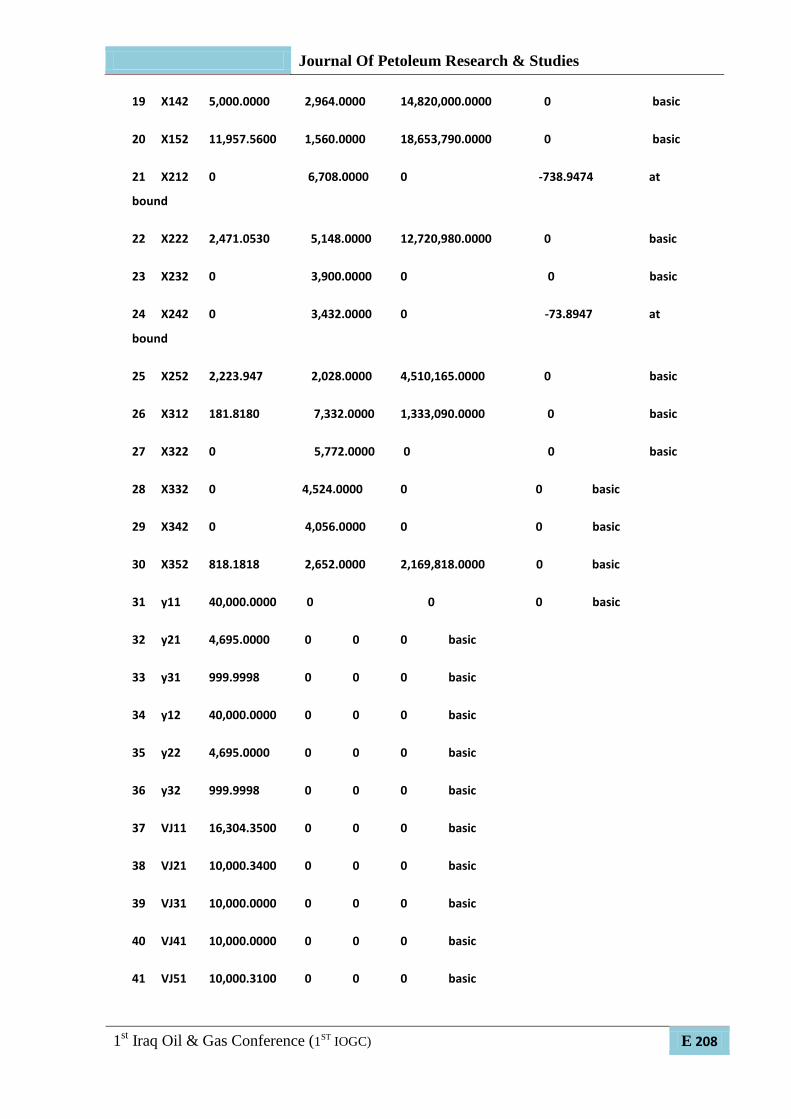
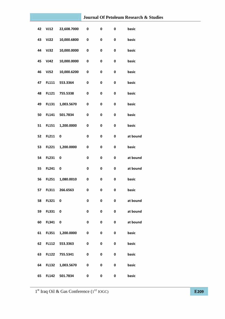
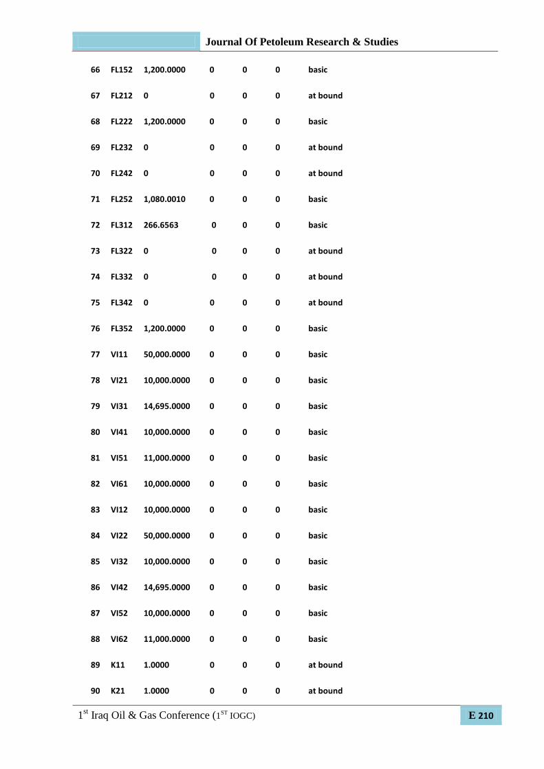
Financial risk analysis of the results is employed utilizing Quantitative System

for Business under windows (WINQSB) software. The output of this level will

be regarded as production guidelines and utilize as input for the next level

(scheduling level) as shown in figure (3.1).

3.2.2 The Planning Level (Linear Goal Programing)

The company may be has multi objectives, therefore, linear goal

programming will be use and formulated according to priorities of these goals

(Ranked Goals) to maximize or minimize deviation variables in goal

constraints. Therefore, some constraints must be modifying to be goal

constraints like (1a) and (8a) and the others stay as it formulated.

I ∑ yiH +MADgh -MIDgh= ddHt (1b) i

The constraint (2) states there are multi objectives in LGP model where the

MADi, MIDi represents variable deviations.

I I J J

∑price yih -∑∑prf xijh-∑palty Sjh+MADgh-MIDgh=0 (8b) i i j j

The objective function will minimize the deviation variables according to

planning goals.



ST IOGC) E185

3.3.3 The scheduling level

In this level the output of the

planning model will be utilized as

input to the scheduling model.

Applying an MILP model, discrete

time representation that assumes that

the entire scheduling horizon is

divided into a finite number of

consecutive time slots (each interval

equal 1day). The beginning time of

each time slot of the scheduling

horizon is (8 AM) with two days time

horizon. The constraints of this level

formulated as follow

3.3.3.1 Material Balance Equation For Components

The amount of component j in tank z at event point t + 1(VJ jzt +1) is

equal to that at event point t (inijzt) adjusted by any amounts transferred from

production unit Fjet and/or delivered to the blender at event point t (∑ xijt).

This relation is expressed by constraint (8). Constraint (9) imposes that the

target flow Fljzt should be between the upper and lower bounds of the flow

rates of component j transferred from tank z to the blender.

J

VJ jzt +1 = inijzt + Fetjt −∑ xijt (8) j

Fl min jzt Ait ≤ Fljzt ≤ Flmax jzt Ait (9)

The constraint (10) imposes the target flow for component j to be equal to the

minimum flow rate plus slack variable multiplied by component percentage .

Fljzt - Fl min jzt - CPjit SLjzt ≥ 0 (10)



ST IOGC) E 186

3.3.3.2 Volumetric Component Concentration Constraints

Constraint (11) is to ensure that volumetric component concentration

that maintains the solution feasible to produce the demand at the satisfied

quality and quantity.

x ijt ≤ con jit (11)

3.3.3.3Component Storage Capacity

Constraint (12) imposes a volume capacity limitation of component j in

component tank z at event point t.

Vmin jzt ≤ VJ jzt ≤ Vmax jzt (12)

3.3.3.4 Product Composition Constraint

Constraint (13) imposes that the blended product i will be equal or less

than the summation of its blended components j at time slot t.

I J

∑(∑ x ijt = y it ) (13)

i j



ST IOGC) E187

3.3.3.5 Product Constraints

Constraint (14) impose the blended product will be equal to or more

than satisfied demand for product i in time t and equal or less than maximum

capacity of product tank.

T I

∑∑ Sdit ≤ yist≤ MCist (14) t i

3.3.3.6 Assignment constraint

Constraint (15) impose that the summation of binary variable Ait

should be equal to or less than the maximum number of blender Nt that can be

working in parallel during time slot t:

I ∑ A it ≤ Nt (15) i

Constraint (16) imposed the blended product yit will be equal to or less than

the result of multiplying binary variable kit by satisfied demand Sddt to due

date.

I

∑yit ≤ Sddt(kit) (16) i

Constraint (17) imposed the blended product yit will be equal to or less than

the result of multiplying binary variable kit by satisfied demand Sddt to due

date.



ST IOGC) E 188

I ∑yit≤ Sddt (Ait) (17) i

3.3.3.7 Material Balance Equation For Products Tanks

Constraints (18) & (19) express that the volumetric amount of product i

in tank s at event point t+1 is equal to that at event point t adjusted by any

amounts transferred from the blender - the lifted amount at event point t.

I S

∑∑(VI ist+1 = ini ist+ y ist(kit) - Sd isd(1-kit) for s=1,3,5 t=1 (18a) i s

I S

∑∑(VI ist+1 = ini ist+ y ist(1-kit) - Sd isd(kit) for s=1,3,5 t=2 (18b) i s

I S

∑∑ (VI ist +1= ini ist +y ist (1-kit) - Sd isd (kit) for s=2, 4, 6 t=1 (19b) i s

I S

∑∑ (VI ist +1= ini ist +y ist (kit) - Sd isd (1-kit) for s=2, 4, 6 t=2 (19b) i s

3.3.3.8 Product Storage Capacity

Constraint (20) imposes a volume capacity limitation of product i in

product tank at event point t. Constraint (21) imposes the target flow Flist



ST IOGC) E189

should be between the upper and lower bounds of the flow rates of product

transferred from tank s to the customer.

Vmin ist ≤ VI ist ≤ Vmax ist (20)

Fll min izt kit ≤ Fllizt ≤ Fllmax izt kit (21)

The constraint (22) imposes the target flow for product i that is equal to the

minimum flow rate plus slack variable.

Fllist - Fll min ist - SLList ≥ 0 (22)

An additional set of variables and equations is required to define penalties

that can be added to the objective function of the proposed model. These

penalties can partially relax some hard problem specifications that can generate

infeasible solution when real world problems are addressed.

Constraint (23) will satisfy quality requirements.

I J J

∑ ((∑qj xij )-( ∑xij Qi) ≥ 0 ) (23)

i j j

3.3.3.9 Penalty For Intermediate Product Shortage

A common source of infeasible solutions is the surplus amount of

component required to satisfy either predefined component concentration or

certain market specifications. Intermediate products can be purchased or sold at

negative cost from a third-party. The continuous variable Si,t defines the



ST IOGC) E 190

amount of intermediate product j needed in time slot t, to relax minimum

inventory constraints:

J

VJ jzt = inijzt + Fet j - ∑xijt + Sjt (24)

j

The penalty term (25) is directly proportional to the component purchase cost

as show below:

T I

p = ∑ ∑ (pltysj Sit) (25)

t i

3.3.3.10 Penalty For Demand Deviation

Due to the uncertainty demand, penalty may be added to the production

cost and the constraints (26) & (27). The required demand will be equal to or

less than the amount of blended product plus initial product in storage tank plus

the amount of product purchased from a third party to satisfy the demand.

I

∑(Inii t + yit + Dd− it ≥ Sd id) (26)

i

I

∑(Inii t + yit - Dd+ it ≥ Sd id) (27)

i

The constraint (28) imposes the generated penalty of demand.

I I

p =∑ pltydit Dd− it + ∑ pltydit Dd+ it (28)

i i



ST IOGC) E191

3.3.3.11 Objective Function

While satisfying all quality and logistic issues, the main objective of

the scheduling model is to maximize the net profit. Constraint (29) is to

maximize the result of the summation of contribution profit for each

component used to satisfy the required demand minus the summation of

penalty:

T I J P

Max ∑ ∑ ∑ pfij Xijt - ∑p + SLjt +SLLit (29)

t i j p

The proposed model will be employed and tested for three different case

studies employing the available resources at AL-Dura Refinery.

4. Case Study

In the near future a series of development processes in AL-Dura

refinery, two conversion units will be constructed. Therefore, the refinery may

produce three grades of gasoline regular, premium and supper (y1, y2 and y3)

with different octane numbers (87, 89 and 93) for the demand of (280000,

105000 and 77000). The tables below show the required data. By the proposed

approach, it is possible to define optimum operation plan and then schedule the

results, if the refinery is committed is to satisfy 7000 bpd of product y1 and

170000 bpd of product y3 according to customers demand. Figure (4) shows the

systematic representation for this case study.



ST IOGC) E 192

Fig. (4) show program solution window

Table (1) Intermediate product data

Cost

ID

RVP

PSI

ON Quantity

Barrel

Symbol Material Seq.

10140 11 66 12000 X1 Light

naphtha

1

11700 8 80 10000 X2 Power

former

2

12948 17 88 10000 X3 Ismorate 3

13416 10 90 5000 X4 Reformat 4

14820 5 99 15000 X5 CCR 5



ST IOGC) E193

Table (2) data for the required product (daily demand)

Due date Price

B.ID

Daily

Demand

barrel

RVP

psi.

ON product

8am 16380 40000 13 87 Y1

2pm 16848 15000 11 89 Y2

11am 17472 11000 11 93 Y3

Table (3) intermediate tank data

Max

flow

B/hr

Min

flow

B.hr

Max

volume

B.

Min

volume

B.

Capacity

B.

Material Tank

number

1200 100 73000 10000 73000 Light

naphtha

TK 1

1200 100 73000 10000 73000 Power

former

TK 2

1200 100 73000 10000 73000 Ismorate TK 3

1200 100 73000 10000 73000 Reformat TK4

1200 100 73000 10000 73000 CCR TK5

Table (4) Product tank data

Max

flow

Min

flow

Max

volume

Min

volume

capacity Material Tank

number

2000 250 73000 10000 73000 REGULAR TK6

2000 250 73000 10000 73000 REGULAR TK7

2000 250 73000 10000 73000 PREMIUM TK8

2000 250 73000 10000 73000 PREMIUM TK9

2000 250 73000 10000 73000 SUPPER TK10

2000 250 73000 10000 73000 SUPPER TK11



ST IOGC) E 194

4.1 The Planning Model

The developed model

employs (LP) at the planning level &

employs (WIN QSP system version

1.00) run on widow XP, As shows in

figure (5) The results generated at

this level are shows in table (5) and

Figure (6).

Table (5) shows the expected

profit, which comes from selling

280,000 bbl of regular gasoline,

32,869 bbl of premium gasoline and

7000 bbl of supper gasoline weakly.

Therefore, the refinery throughput

will be 45695 bpd of three grades of

gasoline product according to due

date, the residue of intermediate

product (naphtha) reach to 6,304 bpd.

Therefore, in order to reduce the

surplus naphtha, the refinery has two

choices, either to use additives to

produce high grade gasoline, or

minimize naphtha production to

6,304 bpd.

The solution is optimum,

when unit profit of light

naphtha product ranges from

(6,240 to 12688 ID) Also If

unit profit of reformat ismorat

ranges from (3,138 to 3,432

ID) And if unit profit of

reformat ranges from (2,964

ID o maximum positive

value) Figure (7) shows the

optimum recipe for each

product.

The net profit will be sensitive by

2,523 ID to any decrease or increase

of one barrel of power former since

its quantity stay between 16,000 to

142,500 bbl, and sense 3,608 ID also

in any decrease or increase of one

barrel of ismorat since its quantity

stay between 35,636 to 116,136 bbl.

Also sense 3,723 ID by any decrease

or increase by one barrel of reformat

since its quantity stay between 3500

to 77,291 bbl, and sense 4,944 ID

also in any decreasing or increasing

by one barrel of power former since

its quantity stay between 82,090 to

135,757 bbl.



ST IOGC) E195

Fig.(5) WIN QSB input window for case study 3



ST IOGC) E 196

Fig. (6) show program solution window

Table (5) summary solution for case study (4)

Contribution

profit ID.

Profit for

each

barrel ID.

Quantity Products

963,942,800 3,428 280000 Regular

gasoline

117,563,080 3,412 32,869 Premium

gasoline

25,687,200 3,669 7000 Supper

gasoline

- -6240 44,130 Surplus

1,107,193,000 Objective

function



ST IOGC) E197

a) Components percentage of regular gasoline

b) Components percentage of premium gasoline

c) Components percentage of supper gasoline

Fig. (7) optimum recipes for different gasoline grades

a) Regular gasoline b) premium gasoline c) supper gasoline

4.2 Scheduling Model

The results of the planning

level shown in the previous tables

describe the optimum quantity

decisions for different products

( regular , premium and supper) and

determine the optimum component

concentrations for each product, that

minimize product recipes cost and

meet product specifications. These

results will be used as input to the

scheduling level. The main objective

14%

22%

19%12%

33%naphtha

power former

isomarat

reformat

0%

28%

43%0%

29%NAPHTHA

POWER FORMER

ISO

REFORMAT

CCR

0% 3%

49%

0%

48%

naphtha

POWER FORMER

ISO

REFOMAT

CCR



ST IOGC) E 198

of the second level is to minimize

inventory holding and operational

cost subject to product due date, that

occur by release of an optimum time

table for each part of blending

system. The optimum timing

decisions maximize the utilization of

product and component tanks that

take into consideration the due date

of product. Appendix A shows

scheduling results. The Gantt chart of

figure (8) shows the summary of

intermediate product flow rates for

three products for two days schedule.

Figure (9) shows a summary of

product tanks for three products of

two days schedule. The next tables

shows more details of flow rate for

intermediate product tanks for

different gasoline grades for two days

scheduling horizon.

Fig. (8) Gantt chart showing two days scheduling for intermediate tanks flow rate



ST IOGC) E199

Table (6) Summary of intermediate tanks schedule for regular gasoline

Tan

k n.

Compone

nt

Start

period

invento

ry

Flo

w

seq.

Flo

w

B.h

r

Starti

ng

time

Endin

g

time

End

period

invento

ry

TK

1

Light

naphtha 10000

Fl

111

519.

7 9pm 8am 16304

TK

2

Power

former 10000

Fl

121 791 9pm 8am 10000

TK

3 Isomerat 10000

Fl13

1 683 9pm 8am 10000

TK

4 reformat 10000

Fl

141

456.

2 9pm 8am 10000

TK

5 CCR 10000

Fl

151

120

0 9pm 8am 10000

As shown in table (6) to

produce regular grade of gasoline,

its need at least 11 hours to blend

the required quantity by blend five

components. The flow rat of light

naphtha will be 519.7 barrel per

hour, for power former the flow

rate 791 barrel per hour, for

ismorat 683 barrel per hour, for

reformat 456.2 barrel per hour and

for CCR component will be 1200

barrel per hour.

To produce premium gasoline

table (7) shows its need 1:40 hours

to blend the required quantity of

product and use three components.

The flow rat of power former

component will be 771 barrel per

hour, for ismorat will be 1200

barrel per hour and for CCR

component will be 814.2 barrel per

hour.

Finally to produce supper

gasoline 25 minutes need by use



ST IOGC) E 200

three components the flow rate of

power former will be 74.8 barrel

per hour, for ismorat 1200 barrel

per hour and for CCR component

will be 1162.6 barrel per hour.

Table (7) Summary of intermediate tanks schedule for premium gasoline

Ta

nk

n.

Componen

t

Start

inventor

y

Flo

w

seq.

Flo

w

B.

hr

Start

time

End

time

End

period

inventory

TK

1

Light

naphtha 10000

Fl

211 0

12:20p

m 2pm 16304

TK

2

Power

former 10000

Fl

221

77

1

12:20p

m 2pm 10000

TK

3 Isomerat 10000

Fl2

31

12

00

12:20p

m 2pm 10000

TK

4 reformat 10000

Fl

241 0

12:20p

m 2pm 10000

TK

5 CCR 10000

Fl

251

81

4

12:20p

m 2pm 10000



ST IOGC) E201

Table (8) Summary of intermediate tanks schedule for supper gasoline

Tan

k n.

Compone

nt

Start

period

invento

ry

Flo

w

seq.

Flo

w

.hr

Startin

g time

Endin

g

time

End

period

invento

ry

TK

1

Light

naphtha

10000 Fl

311

0 10:35a

m

11am 16304

TK

2

Power

former

10000 Fl

321

74.

8

10:35a

m

11am 10000

TK

3

Isomerat 10000 Fl33

1

120

0

10:35a

m

11am 10000

TK

4

reformat 10000 Fl

341

0 10:35a

m

11am 10000

TK

5

CCR 10000 Fl

351

116

2

10:35a

m

11am 10000

Table (9) Summary of Product tanks schedule for two days

Product

name

Tank

number

End period

inventory

(first day )

End period inventory

(second day)

Regular TK6 50000 10000

TK7 10000 50000

Premium TK8 14000 10000

TK9 10000 14000

Supper TK10 11000 10000

TK11 10000 11000



ST IOGC) E 202

Fig. (9) Gantt chart scheduling for intermediate tanks

Table (10) summary for blender’s schedule

Blen

ders Product

D

a

y

Starting

time

Ending

time

Product

quantity/

barrel

B1

Regular

G. 1 10pm 8am 40000

= 2 10pm 8am 40000

B2

Premium

G. 1 12pm 2pm 4695

= 2 12pm 2pm 4695

B3

Supper

G. 1 10:19am 11am 1000

= 2 10:19am 11am 1000



ST IOGC) E203

5. Conclusion And Futuer Recommendation

In the current case the

proposed approach employed to

express the ability to produce regular

and premium of gasoline without

additives. If refinery produce supper

grade of gasoline, this will generate

surplus of intermediate products.

Therefore to produce high grade of

gasoline without additives and

surplus in intermediate product, the

refinery should include an additional

conversion unit to improve the light

naphtha of more than 95ON with

capacity at least 5000 bpd.

The conclusions of this work are as

follow:

1. The proposed approach avoids some

assumptions that make the model

unrealistic; therefore, the proposed

approach is applicable in real world.

2. For the complex case study the

results of the proposed approach (LP

& MILP model) were gained after

0.031 second CPU time for planning

level and after 3.375 second CPU

time for scheduling level.

3. The current work was applied to

gasoline product and fuel oil, but

can also be applied for all blended

refinery products like gas oil,

lubricants, jet fuel etc…

4. The proposed approach has the

ability to assess the financial risk

that occurs by uncertain inputs.

5. The proposed approach utilizes the

Linear Goal Programming (LGP)

and Linear Programming (LP)

efficiently.

6. The developed approach has high

efficiency and flexibility for short-

term planning and scheduling in oil

refinery.

7. The proposed approach minimize

lead time by reduce reblend

process .



ST IOGC) E 204

It‟s a continuation to this work,

the followings are

recommendation:

1. The number of grades of some

products may exceed 18 types in

AL-Dura refinery, therefore, when

utilizing the proposed approach the

developments of the scheduling

level are necessary to impose the

sequencing in the blender to

produce different products.

2. For a company like MRC that has

many demand areas and many

refineries. It is important to

integrate a network for product

blending and distribution to

minimize the bottleneck in some

refineries therefore model for multi

refineries planning is needed.

3. Uncertainty becomes a common

aspect therefore, integrating crude

supply, blending, and a product

distribution model in refinery

planning under uncertainty is

needed.

4. Integrating the related process is

necessary to avoid the financial

risk generated by the

decomposing; therefore, financial

risk management in the scheduling

of refinery operations.

5. Inventory problem has grown

recently in AL-Dura Refinery

according to development process

therefore it‟s important to study

inventory management under

uncertainty.



ST IOGC) E205

Refernces

1. Ming Li Qiqiang , Tian Xin , (2009) Scheduling Optimization of Refinery

Operations Based on Production Continuity, Proceedings of the IEEE

International Conference on Automation and Logistics Shenyang, China

Vol 55--PP4244-4795

2. Dayadeep S. Monder, (2001) Real-Time Optimization of Gasoline

Blending with Uncertain Parameters . MSc. Thesis. University of Alberta,

Canada .

3. Cuiwen Cao a, Xingsheng Gu a, (2009) Chance Constrained Programming

Models for Refinery Short-term Crude Oil Scheduling Problem, App. Math.

Mod,Vol. 33,PP. 1696–1707.

4. J. D. Kelly , (2006) Logistics: the Missing Link In Blend Scheduling

Optimization , .Hydrocarbon Processing, pgs 45 –51.

5. Hansa Lakkhanawat , Miguel J. Bagajewicz, . (2008) Financial Risk

Management with Product Pricing in the Planning of Refinery Operations

Ind. Eng. Chem. Res,Vol 47, pp. 6622–6639.

6. J. Hancsok , Sz. Magyar , and Valkai, (2009) Investigation of the

Production of Gasoline Blending Component Free of Sulfur. petr. & and

coal, Vol. 45, PP. 3-4, 99-104.

7. Klaus Glismann, &Gu¨ nter Gruhn, (2001)Integrated Planning and

Scheduling for Blending Processes. Comp. & Chem. Eng. Vol. 20.pp. 109–

128

8. Rois Fatoni,(2009) Modeling and Optimization of Refinery Gasoline

Blending Ind. Eng. Chem. Res, Vol 50 ,PP. 4475-4482

9. Cheng Seong Khor, (2006) A Hybrid of Stochastic Programming

Approaches with Economic and Operational Risk Management for



ST IOGC) E 206

Petroleum Refinery Planning under Uncertainty , MSc. Thesis, Waterloo,

Ontario, Canada,

10. Arkadej Pongsakdi , (2006) Pramoch , and Miguel J. Bagajewicz,

Financial Risk Management in the planning of refinery operations, Int. J.

Pro.& Eco. Vol.103, PP. 64–86.

11. Khalid Y. Al-Qahtani, (2009). Petroleum Refining and Petrochemical

Industry Integration and Coordination under Uncertainty. PhD Dissertation

University of Waterloo, Canada.

12. Naiqi WU, MengChu Zhou , (2005) Short-term Scheduling for Refinery

Process: Bridging the Gap between Theory and Applications, international

journal of intelligent control and system. Vol. 10, No. 2, pp. 162-174.

13. Khalid Y. AL-Qahtani and Ali Elkamel , (2010) “Planning and Integration

of Refinery and Petrochemical Operations” , Wiley-vch Verlag GmbH &

Co. KGaA, Weinheim .

14. James H. Gary Glen, (2007) E. Hadwerk Mark, “Petroleum Refining

Technology and Economic, CRC press , Fifth edition. USA.

15. Zukui Li, (2010) Process Operations with Uncertainty and Integration

Considerations, PhD Dissertation , The State University of New Jersey,

USA

16. Surinder Parkash , (2003) "Refining Process Handbook” Gulf Professional

Publishing of Elsevier, USA. Second edition.

17. Edward C. bodington, , (1995) “Planning Scheduling and Control

integration in the process industry” McGraw-Hill, USA.



ST IOGC) E207

APPENDIX A

Combined Report for product scheduling

04:11:37 Sunday July 03 2011

Decision Solution Unit Cost or Total Reduced

Basis

Variable Value Profit c(j) Contribution Cost Status

1 X111 5,513.8330 6,240.0000 34,406,320.0000 0 basic

2 X121 7,528.6040 4,680.0000 35,233,870.0000 0 basic

3 X131 10,000.0000 3,432.0000 34,320,000.0000 0 basic

4 X141 5,000.0000 2,964.0000 14,820,000.0000 0 basic

5 X151 11,957.5600 1,560.0000 18,653,790.0000 0 basic

6 X211 0 6,708.0000 0 -737.8469 at bound

7 X221 2,471.0530 5,148.0000 12,720,980.0000 0 basic

8 X231 0 3,900.0000 0 0 basic

9 X241 0 3,432.0000 0 -73.5947 at

bound

10 X251 2,223.9470 2,028.0000 4,510,165.0000 0 basic

11 X311 181.8180 7,332.0000 1,333,090.0000 0 basic

12 X321 0 5,772.0000 0 0 basic

13 X331 0 4,524.0000 0 0 basic

14 X341 0 4,056.0000 0 0 basic

15 X351 818.1818 2,652.0000 2,169,818.0000 0 basic

16 X112 5,513.8310 6,240.0000 34,406,300.0000 0 basic

17 X122 7,528.6100 4,680.0000 35,233,900.0000 0 basic

18 X132 10,000.0000 3,432.0000 34,320,000.0000 0 basic



ST IOGC) E 208

19 X142 5,000.0000 2,964.0000 14,820,000.0000 0 basic

20 X152 11,957.5600 1,560.0000 18,653,790.0000 0 basic

21 X212 0 6,708.0000 0 -738.9474 at

bound

22 X222 2,471.0530 5,148.0000 12,720,980.0000 0 basic

23 X232 0 3,900.0000 0 0 basic

24 X242 0 3,432.0000 0 -73.8947 at

bound

25 X252 2,223.947 2,028.0000 4,510,165.0000 0 basic

26 X312 181.8180 7,332.0000 1,333,090.0000 0 basic

27 X322 0 5,772.0000 0 0 basic

28 X332 0 4,524.0000 0 0 basic

29 X342 0 4,056.0000 0 0 basic

30 X352 818.1818 2,652.0000 2,169,818.0000 0 basic

31 y11 40,000.0000 0 0 0 basic

32 y21 4,695.0000 0 0 0 basic

33 y31 999.9998 0 0 0 basic

34 y12 40,000.0000 0 0 0 basic

35 y22 4,695.0000 0 0 0 basic

36 y32 999.9998 0 0 0 basic

37 VJ11 16,304.3500 0 0 0 basic

38 VJ21 10,000.3400 0 0 0 basic

39 VJ31 10,000.0000 0 0 0 basic

40 VJ41 10,000.0000 0 0 0 basic

41 VJ51 10,000.3100 0 0 0 basic



ST IOGC) E209

42 VJ12 22,608.7000 0 0 0 basic

43 VJ22 10,000.6800 0 0 0 basic

44 VJ32 10,000.0000 0 0 0 basic

45 VJ42 10,000.0000 0 0 0 basic

46 VJ52 10,000.6200 0 0 0 basic

47 FL111 553.3364 0 0 0 basic

48 FL121 755.5338 0 0 0 basic

49 FL131 1,003.5670 0 0 0 basic

50 FL141 501.7834 0 0 0 basic

51 FL151 1,200.0000 0 0 0 basic

52 FL211 0 0 0 0 at bound

53 FL221 1,200.0000 0 0 0 basic

54 FL231 0 0 0 0 at bound

55 FL241 0 0 0 0 at bound

56 FL251 1,080.0010 0 0 0 basic

57 FL311 266.6563 0 0 0 basic

58 FL321 0 0 0 0 at bound

59 FL331 0 0 0 0 at bound

60 FL341 0 0 0 0 at bound

61 FL351 1,200.0000 0 0 0 basic

62 FL112 553.3363 0 0 0 basic

63 FL122 755.5341 0 0 0 basic

64 FL132 1,003.5670 0 0 0 basic

65 FL142 501.7834 0 0 0 basic



ST IOGC) E 210

66 FL152 1,200.0000 0 0 0 basic

67 FL212 0 0 0 0 at bound

68 FL222 1,200.0000 0 0 0 basic

69 FL232 0 0 0 0 at bound

70 FL242 0 0 0 0 at bound

71 FL252 1,080.0010 0 0 0 basic

72 FL312 266.6563 0 0 0 basic

73 FL322 0 0 0 0 at bound

74 FL332 0 0 0 0 at bound

75 FL342 0 0 0 0 at bound

76 FL352 1,200.0000 0 0 0 basic

77 VI11 50,000.0000 0 0 0 basic

78 VI21 10,000.0000 0 0 0 basic

79 VI31 14,695.0000 0 0 0 basic

80 VI41 10,000.0000 0 0 0 basic

81 VI51 11,000.0000 0 0 0 basic

82 VI61 10,000.0000 0 0 0 basic

83 VI12 10,000.0000 0 0 0 basic

84 VI22 50,000.0000 0 0 0 basic

85 VI32 10,000.0000 0 0 0 basic

86 VI42 14,695.0000 0 0 0 basic

87 VI52 10,000.0000 0 0 0 basic

88 VI62 11,000.0000 0 0 0 basic

89 K11 1.0000 0 0 0 at bound

90 K21 1.0000 0 0 0 at bound



ST IOGC) E211

91 K31 1.0000 0 0 0 at bound

92 K12 1.0000 0 0 0 at bound

93 K22 1.0000 0 0 0 at bound

94 K32 1.0000 0 0 0 at bound

95 SL1 2,347.6280 1.0000 2,347.6280 0 basic

96 SL2 715.0095 1.0000 715.0095 0 basic

97 SL3 1,323.8200 1.0000 1,323.8200 0 basic

98 A11 1.0000 0 0 0 at bound

99 A21 1.0000 0 0 0 at bound

100 A31 1.0000 0 0 0 basic

101 A12 1.0000 0 0 0 at bound

102 A22 1.0000 0 0 0 at bound

103 A32 1.0000 0 0 0 basic

104 N1 3.0000 0 0 0 basic

105 N2 3.0000 0 0 0 basic

Objective Function (Max.) = 316,340,400.0000



ST IOGC) E 212

Nomenclature

Indices

d due dates of product demands

j intermediate product (component)

i final products or gasoline grades

t time slots

p penalty

s product tank

z component tank

Sets

D= set of product due dates

J= set of intermediates or components to be blended

I= set of final products

T= set of time slots

P= set of penalties

S= set of product tanks

Z= set of component tanks

Parameters

PFj = profit of component j.

PFi = profit of product i .

dt = demand due date in time slot t.

dd ih = the required demand for product i at time horizon H.

dd it = the required demand for product i at time slot t.

ddcih = minimum demand must be satisfy at time horizon h.



ST IOGC) E213

ddcit = minimum demand must be satisfy at time slot t

cpijt= component percentage in product i.

et = duration of time slot t .

Fj = constant flow rate of components from production units.

H = time horizon.

AV jh= availability of component j in time horizon h.

AV jt= availability of component j in time t.

Fllmax it = maximum flow rate of product i.

Fllmin it = minimum flow rate of product i.

Flmax j = maximum component j flow rate required to produce product i in due

date t.

Flmin j = minimum component j flow rate required to produce product i in due date

Qi= the required property for product i

qj= the required property for component j

con j,i =volumetric amount of component j in product quantity .

st = predefined starting time of time slot t.

Vmax jzt = maximum storage capacity of component j in tank z at time t.

Vmin jzt = minimum storage capacity of component j in tank z at time t.

Vmax ist = maximum storage capacity of product I in tank s at time t.

Vmin i st = minimum storage capacity of product i in tank s at time t.

pltysj= penalty cost for purchasing or selling component j from third party.

Pltydit =penalty cost for unsatisfied demand for product i.

Binary Variables

Ait = binary variable denoting that product i is blended in time slot t



ST IOGC) E 214

Kist = binary variable denoting that product i is lifted form tank s in time t

Integer variable

Nbt = maximum number of blenders that can be working in parallel in time slot t.

Continues Variables

xijh = amount of volumetric quantity of component j being transferred to produce

product i at time horizon h .

xijt = amount of volumetric quantity of component j being transferred to produce

product i at time slot t .

yih= amount of volumetric quantity of product i being blended in time horizon h.

yit= amount of volumetric quantity of product i being blended in time t.

ini jzt = initial inventory of component j in tank z at event point t.

ini ist = initial inventory of product I in tank s at event point t.

S jt = amount of component j to be purchased or sold in time slot t.

Dd-it= amount of product purchase product from third party to satisfy demand

Dd+it= amount of surplus product i at time slot t.

Sh= surplus of the available component j at time horizon h .

SLjt= slack variable for component flow rate at time slot t.

SLLit= slack variable for product quantity at time slot t.

MADgh = goal deviation to minimize unsatisfied goal at time horizon h.

MIDgh= goal deviation to maximizes unsatisfied goal at time horizon h.

Fljz t=target flow for component j from tank z at time slot t.

Fllist=target flow for product i from tank s at time slot t.

Date post:	27-Jan-2022
Category:	Documents
Upload:	others
View:	3 times
Download:	0 times

Short Term Planning and Scheduling For Gasoline Blending ...

Documents