Short-Term Voltage Stability Analysis for Power System with Single-Phase Motor
Load
By
Yan Ma
A Thesis Presented in Partial Fulfillment of the Requirements for the Degree
Master of Science
Approved April 2012 by the Graduate Supervisory Committee:
George G. Karady, Chair
Vijay Vittal Raja Ayyanar
ARIZONA STATE UNIVERSITY
May 2012
i
ABSTRACT
Voltage stability is always a major concern in power system operation.
Recently Fault Induced Delayed Voltage Recovery (FIDVR) has gained increased
attention. It is widely believed that the motor-driven loads of high efficiency, low
inertia air conditioners are one of the main causes of FIDVR events.
Simulation tools that assist power system operation and planning have
been found insufficient to reproduce FIDVR events. This is because of their
inaccurate load modeling of single-phase motor loads. Conventionally three-phase
motor models have been used to represent the aggregation effect of single-phase
motor load. However researchers have found that this modeling method is far
from an accurate representation of single-phase induction motors.
In this work a simulation method is proposed to study the precise
influence of single-phase motor load in context of FIDVR. The load, as seen the
transmission bus, is replaced with a detailed distribution system. Each
single-phase motor in the distribution system is represented by an equipment-level
model for best accuracy. This is to enable the simulation to capture stalling effects
of air conditioner compressor motors as they are related to FIDVR events.
The single phase motor models are compared against the traditional three
phase aggregate approximation. Also different percentages of single-phase motor
load are compared and analyzed.
Simulation result shows that proposed method is able to reproduce FIDVR
events. This method also provides a reasonable estimation of the power system
voltage stability under the contingencies.
ii
ACKNOWLEDGEMENTS
I express my appreciation to many professors and colleagues who have
instructed me and provided helpful suggestions for my work. The contribution of
Dr. George Karady and Dr. Vijay Vittal are particularly valuable. I want to thank
my advisor Dr. George Karady for his valuable guidance throughout the duration
of my study. I also want to thank Dr. Vijay Vittal for his guidance and support
over the entire duration of this thesis. I am deeply indebted to them for all the
fruitful and enlightening discussions.
I want to thank all the members of the power systems group at Arizona
State University for making this experience memorable and enjoyable. Special
thanks to my husband Lloyd Breazeale for his encouragement and support.
iii
TABLE OF CONTENTS
Page
LIST OF TABLES ................................................................................................. vi
LIST OF FIGURES .............................................................................................. vii
NOMENCLATURE ............................................................................................... ix
CHAPTER
1 INTRODUCTION ............................................................................................... 1
1.1 Background ........................................................................................ 1
1.2 Motivation .......................................................................................... 1
1.3 Research scope and objective ............................................................ 2
1.4 Thesis organization ............................................................................ 3
2 VOLTAGE STABILITY ...................................................................................... 5
2.1 What is voltage stability? ................................................................... 5
2.2 Voltage stability categorization .......................................................... 6
2.3 Voltage stability analysis methods ..................................................... 7
2.4 Voltage stability indices ..................................................................... 8
2.4.1 Security margin .......................................................................... 9
2.4.2 Voltage collapse indicator ......................................................... 10
2.5 FIDVR phenomenon ........................................................................ 12
3 POWER SYSTEM LOAD MODELING .......................................................... 15
3.1 Overview .......................................................................................... 15
3.2 Load model category ........................................................................ 16
3.2.1 Static load model ...................................................................... 16
iv
CHAPTER Page
3.2.2 Dynamic load model ................................................................ 18
3.2.3 Composite load model .............................................................. 19
3.3 Load model approaches ................................................................... 20
3.3.1 Measurement based .................................................................. 20
3.3.2 Component based ..................................................................... 20
3.4 Induction motor ................................................................................ 21
3.4.1 Three-phase induction motor .................................................... 21
3.4.2 Single-phase induction motor ................................................... 28
3.4.3 Particular characteristics of induction motor load .................... 35
4 MODELING and SIMULATION of RESIDENTIAL AIR CONDITIONERS . 36
4.1 Introduction of residential air conditioner (RAC) motors ............... 36
4.2 Why modeling RAC motors are important ...................................... 37
4.3 Model requirements ......................................................................... 38
4.4 Modeling RAC compressors ............................................................ 39
4.4.1 Classification of RAC models .................................................. 39
4.4.2 Phasor model ............................................................................ 39
4.4.3 Grid-level models ..................................................................... 43
4.5 Motor modeling and parameters ...................................................... 45
4.5.1 Single-phase induction motor parameters and simulation........ 45
4.5.2 Three-phase induction motor parameters and simulation ........ 48
5 PROPOSED METHOD ..................................................................................... 52
5.1 Overview .......................................................................................... 52
v
CHAPTER Page
5.2 Proposed method for simulation of single-phase induction motor .. 52
5.3 Simulation software ......................................................................... 54
6 CASE STUDIES ................................................................................................ 55
6.1 Overview .......................................................................................... 55
6.2 The transmission system .................................................................. 57
6.3 Simulation cases............................................................................... 57
6.3.1 Three-phase motor load ............................................................ 58
6.3.2 Single-phase motor load ........................................................... 61
6.4 Case analysis .................................................................................... 68
6.4.1 10% motor load ........................................................................ 69
6.4.2 30% motor load ........................................................................ 71
6.4.3 50% motor load ........................................................................ 72
6.4.4 70% motor load ........................................................................ 74
7 CONCLUSIONS AND FUTURE WORK ........................................................ 76
7.1 Conclusions ...................................................................................... 76
7.2 Future work ...................................................................................... 78
REFERENCES ..................................................................................................... 79
APPENDIX
A DISTRIBUTION SYSTEM SIMULATION ..................................................... 84
B DATA EXCHANGE PROGRAM ..................................................................... 88
vi
LIST OF TABLES
Table Page
3.1 Equivalent circuit parameter values of three-phase induction motor ............. 24
3.2 Equivalent circuit parameter values of single-phase induction motor ............ 32
4.1 Parameters for phasor model .......................................................................... 45
4.2 Parameter values of three-phase induction motor ........................................... 48
6.1 Three-phase motor loads on bus 6 .................................................................. 58
6.2 Distribution systems with single-phase motor load ........................................ 62
6.3 Comparison sets for different motor load percentage ..................................... 69
vii
LIST OF FIGURES
Figure Page
3-1 Simplified equivalent circuit of the three-phase induction motor .................. 22
3-2 General characteristics of the three-phase induction motor ........................... 24
3-3 Simplified equivalent circuit of the single-phase induction motor ................. 30
3-4 General characteristics of the single-phase induction motor .......................... 32
4-1 Simulation result of phasor model .................................................................. 47
4-2 Simulation result of three-phase motor model ............................................... 50
5-1 The simulation procedure of the power system .............................................. 53
6-1 Distribution system with single-phase motor load ......................................... 56
6-2 Bus 6 load power for three-phase motor load ................................................. 59
6-3 Bus 6 voltage magnitude for three-phase motor load ..................................... 60
6-4 Bus 6 voltage angle for three-phase motor load ............................................. 61
6-5 Bus 6 load power with protection setup 1 ...................................................... 63
6-6 Bus 6 voltage magnitude with protection setup 1 ........................................... 64
6-7 Bus 6 voltage angle with protection setup 1 ................................................... 65
6-8 Bus 6 load power with protection setup 2 ...................................................... 66
6-9 Bus 6 voltage magnitude with protection setup 2 ........................................... 67
6-10 Bus 6 voltage angle with protection setup 2 ................................................. 68
6-11 Bus 6 load apparent power for 10% motor load ........................................... 70
6-12 Bus 6 voltage magnitude for 10% motor load .............................................. 70
6-13 Bus 6 load for 30% motor load ..................................................................... 71
6-14 Bus 6 voltage magnitude for 30% motor load .............................................. 72
viii
Figure Page
6-15 Bus 6 load for 50% motor load ..................................................................... 73
6-16 Bus 6 voltage magnitude for 50% motor load .............................................. 74
6-17 Bus 6 load for 70% motor load ..................................................................... 75
6-18 Bus 6 voltage magnitude for 70% motor load .............................................. 75
A-1 Simulink step 1 for calculating end voltage after transformer ...................... 85
A-2 Simulink step 2 for calculating load on 69/12.47 transformer ...................... 86
A-3 Simulink step 3 for calculating load applied transmission load bus .............. 87
ix
NOMENCLATURE
AC Alternating current
AGC Automatic generation control
APS Arizona Public Services
AVR Automatic Voltage Regulator
DC Direct current
DOE Department of Energy
EPRI Electric Power Research Institute
FIDVR Fault Induced Delayed Voltage Recovery
GE General Electric Company
IEEE Institute of Electrical and Electronics Engineers
ISO Independent System Operator
LMTF Load Modeling Task Force
NERC North American Electric Reliability Corporation
P Active power
PES Power and Energy Society
PSAT Power System Analysis Toolbox
PSLF Positive Sequence Load Flow Software
Q Reactive power
RAC Residential Air Conditioner
SCE Southern California Edison
SEER Seasonal Energy Efficiency Ratio
SVS Static VAR Source
x
RPM Revolutions Per Minute
TOL Thermal Over Load
ULTC Under Load Tap Changing
V Voltage
WECC Western Electricity Coordinating Council
Z Impedance
ZIP Constant impedance/current/power load
1PH Single-phase
3PH Three-phase
1
CHAPTER 1
INTRODUCTION
1.1 Background
Power systems have developed into one of the largest industries in the
world. Trends of growth have however led to limiting constraints of power system
operation [1]. One of the major concerns is power system stability. General
classifications are rotor angle (synchronous), frequency, and voltage stability [2]
[3].
Voltage stability is the ability of a power system to maintain steady
acceptable voltages at all buses under normal operation after being subjected to a
disturbance [1]. Voltage instability is the absence of voltage stability as it leads to
progressive voltage decrease or increase [3]. Voltage instability and voltage
collapse are sometimes synonymous.
1.2 Motivation
Load characteristics have a strong influence on power system voltage
stability. Since voltage instability is believed to be caused by the shortage of
reactive power, most voltage stability studies are concentrated on predicting the
load’s reactive power and planning reactive power generation.
Induction motor loads have been found to be a major contributing factor to
voltage instability. When the applied voltage on the motor is reduced to a certain
level, as the result of a fault, the motor suddenly requires much more active and
reactive power. In the worst case, if the induction motors stalls, the motor
typically requires around five times more power than in steady state. The
2
increased power requirements lead to further depressed system voltage and
consequently more induction motors may slow or stall. In this situation, either the
system needs more time to recover or the system may experience voltage
collapse.
Recently, there has been a growing concern about a short-term voltage
instability issue termed Fault Induced Delayed Voltage Recovery (FIDVR). The
cause of this phenomenon is believed to be motor-driven loads of Residential Air
Conditioners (RAC).
According to the DOE 1980-2001 appliance report [4], about 55% of US
households have central air-conditioners and about 23% US households have
individual room units. With the significantly increasing demand for RACs,
electric utilities are experiencing more FIDVR events.
Conventionally three-phase motor models have been utilized in simulation
to represent the aggregation effect of all motor loads. However present power
system simulation tools have been found insufficient to reproduce the FIDVR
events. This is due to their inaccurate representation of the single-phase induction
motor.
1.3 Research scope and objective
The objective of this work is to study the influence of the single-phase
motor loads on the power system voltage stability problem. The specific tasks
include:
Develop a modeling method to accurately represent the behavior of
single-phase induction motor load in power system simulation.
3
Design and build in simulation a detailed distribution system with
different percentage of single-phase motor load. Each single-phase
motor will be represented with an equipment-level model.
Create composite load models to represent the distribution systems.
Each composite load model will be composed of a constant impedance
load (static load), and a three-phase motor model (dynamic load) that
represents the aggregation effect of all single-phase motor loads in the
distribution system.
Compare simulation results from the composite load model against the
detailed distribution system while varying the percentage of motor
load.
Investigate the relationship between the percentages of single-phase
motor load and their impact on voltage stability.
1.4 Thesis organization
This thesis includes seven chapters and is organized as follows.
Chapter 2 provides a brief literature review associated with voltage
stability, such as the definition of voltage stability, voltage stability analysis
methods, and the FIDVR phenomenon.
Chapter 3 reviews load modeling in power systems. A brief description is
presented on categorization of loads and a variety of load modeling methods. Also
models for three-phase and single-phase induction motors are presented.
Chapter 4 introduces characteristics of the RAC and explains why it is
important to model RACs in power system simulation. A variety of RAC models
4
are also discussed. A literature survey is presented on current research in
modeling RACs for power system simulation. Furthermore detailed load models
are introduced for later use in simulation.
In Chapter 5, a method is proposed to study the precise influence of the
RAC motors on the power system.
Chapter 6 presents the results and comparisons of various case studies.
Chapter 7 summarizes the contributions of this research and provides
recommendations for future work.
5
CHAPTER 2
VOLTAGE STABILITY
Voltage stability has imposed more constraints to power system operation
than the past. This is because current power systems are normally operating close
to stability limits. Some large-scale blackouts are believed to have been caused by
voltage instability.
2.1 What is voltage stability?
Generally, voltage stability is defined as the capability of power system to
maintain acceptable voltage at all the buses in the system after being subjected to
a disturbance from a given initial operating condition [1]. Voltage instability is the
absence of the voltage stability and may result in a progressive unacceptable
increase or decrease of voltage of some buses, thus causing load shed and voltage
collapse [3].
Voltage collapse is a dynamic phenomenon usually characterized as a
gradual voltage magnitude decrease and then a sharp accelerated drop after a few
minutes. The fundamental cause of voltage collapse is the inability of the power
system to meet its demand for reactive power [1]. A number of voltage collapse
incidents [3][5][6] have been reported over the past years and are usually caused
by the following major factors:
The fast continuing increase of the load
The insufficient reactive power support
Long transmission line fault or malfunction of its protection
Incorrect adjustment of the Under Load Tap Changer (ULTC)
6
Poor coordination among control and protection devices
Unfavorable load characteristics
Long distance between generators and load
Although voltage magnitude will drop when voltage collapse occurs, a
low voltage at the receiving end does not necessarily indicate a risk of voltage
collapse [7] [8]. On the contrary, in some cases the bus voltage may drop (from
heavy load) while the system is still in stable operation. In other cases voltage
collapse may occur when the bus voltage is still within limits. Consequently, the
study of voltage stability should take into account not only voltage magnitude, but
also other system parameters such as phase angle, admittance matrix, load, and
generator information.
2.2 Voltage stability categorization
Reference [1] and [3] categorize voltage stability in different aspects.
Based on the scale of the disturbance, they are:
Large-disturbance voltage stability. This classification deals with the
capability of the power system to control voltages when subjected to a
large disturbance such as loss of generation or transmission line fault.
Small-disturbance voltage stability is related to the system’s capability
to maintain acceptable voltages when small perturbations occur. The
small perturbations may be the changes in system load, the action of
the system control, etc.
Voltage stability can also be categorized based on the time period.
7
In long-term voltage stability, the range of time period may be a few
minutes to 10’s of minutes. This involves slower systems and
equipment such as AGC, tap-changing transformers, and transformer
saturation.
Mid-term voltage stability is typically in the range of about 10 seconds
to a few minutes. This type of voltage stability includes synchronizing
power oscillation among machines and large voltage or frequency
excursions.
Short-term or transient voltage stability is usually studies in the scale
below 10 seconds. This involves dynamics of fast acting load
components such as induction motors, electronically controlled loads,
and HVDC converters.
2.3 Voltage stability analysis methods
Generally voltage stability analysis can be classified as static or dynamic
[9] [10]. Static analysis entails capturing snapshots of system conditions at an
instant in time. This reduces overall system equations to purely algebraic.
Dynamic analysis utilizes time domain simulation and considers
appropriate dynamic modeling to capture events that lead the system to voltage
instability. The dynamic analysis methods include models of power system
elements that have an influential impact on voltage instability [1].
Compared with static analysis, dynamic analysis provides more accurate
representation of voltage instability. This is useful for detailed study of a specific
system to test coordination, protection and for remedial measures. However,
8
dynamic simulations are more time-consuming than static. This constraint limits
the application of dynamic modeling in studying the bulk power system. In
contrast, static analysis is less computational intensive, and is able to determine
the voltage stability at selected snapshots. If used appropriately, the static method
is able to provide much insight into the nature of the problem and identify the key
contributing elements. Therefore, static analysis is widely utilized for analyzing
voltage stability of bulk power system. In some cases, researchers have combined
both static and dynamic analysis to exploit the advantages of each. Reference [11]
utilizes static analysis to identify the weak elements, and then models them in
more detail with dynamic analysis.
Voltage instability is essentially a nonlinear phenomenon, and it is usually
evaluated using bifurcation theory. Bifurcation theory is the mathematical study
of how and when the solutions to a system change as a result of parameter
changes. Bifurcation theory has the following characteristics when it is applied to
the analysis of voltage stability [5]:
System parameters are assumed to change slowly.
System instability occurs when a small change of system parameters
cause qualitative changes.
In a saddle-node bifurcation, the equilibrium disappears with small
parameter change and consequently the system’s voltage collapses
dramatically.
2.4 Voltage stability indices
Voltage stability indices have been developed to detect proximity of a
9
system to voltage collapse. Voltage stability indices can be used on-line or off-line
to assist the operators in determining how close a system is to voltage instability
and what is the mechanism driving the instability. A good index should have the
following characteristics [9] [12]:
Accurate
Linear
Fast
Providing sufficient information
Simple
Past research on static analysis of voltage stability are generally divided
into two categories.
2.4.1 Security margin
One category entails finding a security margin and the distance the current
equilibrium point is from the instability region. The security margin of a power
system depends on the system’s load margin under normal and contingency
situations. The load margin of the system is defined as the amount of additional
load that would cause a voltage collapse for a particular operating equilibrium [5].
The following indices belong to this category [1]:
Voltage stability index based on V-P characteristics of the system.
System V-P characteristics are the result of several power flow
simulations for different load level at a given power factor. However
V-P characteristics of the system may not predict voltage collapse
correctly because of changing power factor.
10
Voltage stability index based on V-Q characteristics of the system. The
Q-V characteristics of the system show the sensitivity of a bus voltage
to reactive power. The bus being analyzed for its VQ curve is
converted to a PV bus without reactive power limits. The calculation
of VQ curves is time-consuming, and the bus reactive power injection
or absorption is limited in reality. Therefore the Q-V characteristics of
the system are useful but not commonly used for estimating voltage
stability of bulk system.
Voltage stability index based upon the minimal load increment. As
presented in [13], the purpose of this method is to find the minimal
active and reactive power increments that may cause voltage collapse.
The success of this method depends on the initial direction chosen for
loading.
Voltage stability index based on reactive power limit. This was
developed based on the theory that the fundamental cause of voltage
collapse is the incapability of a power system to meet its demand for
reactive power[1].
2.4.2 Voltage collapse indicator
The other category of static analysis is based upon finding a voltage
collapse indicator for which an emergency threshold may be set. Several types are
listed here:
The V-Q sensitivity analysis [14][15] method assumes that P is
constant (∆P=0) at each operating point, and the relationship between
11
∆Q and ∆V is capable of assessing the voltage stability. This method
only works well for small change of operation state.
The Q-V modal analysis method [16] was developed from Q-V
sensitivity analysis. The method computes the eigenvalue and
eigenvector matrix of the reduced Q-V Jacobian marix. Besides
providing estimation of voltage stability, the Q-V modal analysis also
provides information regarding the mechanism of instability. Several
techniques [1][17][18] have been developed to provide fast Q-V model
analysis.
Singular value decomposition analysis [17][19][20][21] was derived
from a linear power flow model based upon the system’s Jacobian
matrix. The method evaluates the distance of the current Jacobian
matrix to becoming singular. This method not only predicts voltage
collapse, but also provides useful information for selecting remedial
control measures.
Voltage Collapse Proximity Indicator (VCPI) [22] assumes that near
maximum loading conditions, small increase in load would require a
significant amount of reactive power due to large line losses. Two
indicators, VCPIp and VCPIq, are used to assess the sensitivity
between total change in generator reactive power and the change in
active and reactive load. The buses with high VCPIp value are the
most effective location for load shielding, and the buses with high
12
VCPIq value are the most effective location for reactive power
compensation.
Voltage Instability Proximity Index (VIPI) [23][24][25]. This method
estimates the voltage instability margin by calculating the angle θ
between the specific vector and the critical vector.
The steady state voltage stability indicator [26] method calculates
indicators for voltage stability of each load bus by solving load flow. It
is able to predict voltage collapse without actually computing load
flows for extreme loading conditions. The stability indicator L is easy
to be calculated with a simple formula and its range is from 0 to 1. The
smaller the L, the more stable the system. This method is widely
utilized.
Some local indicators are for critical parts (nodes or area) of the
system [27][28]. Sometimes system stability only depends on load
change of critical parts (nodes or area). This type of indicator can be
used for on-line voltage stability analysis because of its fast
computation speed.
2.5 FIDVR phenomenon
The FIDVR event is a short-term voltage stability phenomenon. FIDVR
occurs after a system fault. Once the fault has been cleared, the system voltage
remains at the significant low level for several seconds or longer. In [29], NERC
Transmission Issues Subcommittee defined the FIDVR as a voltage condition that
is initiated by a fault and characterized as:
13
Induction motors stall
The voltage is initially recovered to less than 90% of pre-contingency
voltage after the fault has been cleared
The voltage is slowly (more than 2 seconds) restored to the expected
post-contingency steady state voltage levels
FIDVR phenomenon is not new, but most FIDVR events were recently
observed and reported. In [30], Southern California Edison (SCE) Company
described an FIDVR event that occurred in June 1990. This phenomenon
followed fault clearing in the transmission system and involved 1000 square miles.
This paper also mentions the FIDVR observed by Sacramento Municipal Utility
District in August 1990 and by Memphis in 1987. There have been at least eight
FIDVR events in Southeast Florida between 1985 and 1995 [31]. Reference [32]
presents FIDVR events following a multiple contingency fault and breaker failure
at two 230 kV substations in Metro Atlanta. Reference [33] describes an FIDVR
even in 2003 that was initiated by a three-phase fault on the Arizona Public
Services (APS) system. Other FIDVR events are discussed in [34]. These reports
and papers indicate FIDVR is mainly associated with high concentrations of
induction motor loads.
The motors that have contributed to recent FIDVR events are low inertia,
high efficiency, single phase induction motors of Residential Air Conditioners
(RAC). These machines are easy to stall and draw a very high current during stall
state. If the system does not have enough active and reactive power support, the
high power demand of stalled RACs will further deteriorate voltage stability
14
causing more induction motors to stall thus leading to voltage collapse.
Many methods have been proposed to solve FIDVR problem. They can be
categorized as follows [34]:
The customer-level solution entails adjusting the RAC protection
devices to help the RACs overcome or disconnect from the voltage
transient instability. Although RAC manufacturers are hesitant to
modify their standards.
The system solution includes reducing fault clearing time, utilizing
reactive power compensation devices, limiting load with adverse
influence, improving system protection, etc. However since this
method does not necessarily prevent RAC stalling, FIDVR events can
be reduced but not eliminated.
At present, the controlled reactive power support at the grid level is
believed to an efficient method. Also in practice utilities have installed generation
and Static VAR Compensators (SVC) to alleviate FIDVR events.
15
CHAPTER 3
POWER SYSTEM LOAD MODELING
Many techniques and tools have been developed to simulate power system
operation. One of the determining factors for accuracy is correct representation of
power system equipment. However load is the most difficult aspect to model
because of its great diversity.
For appropriate power system planning and operation, detailed load
models are needed. In this chapter, modeling and analysis of electrical motor
loads are introduced. In particular single and three-phase induction motors are
described in detail.
3.1 Overview
As defined in [3], if the load voltages reach post-disturbance equilibrium
after a disturbance, the power system is under stable operation. This definition
also implies that for a stable power system, power generation should match
consumption. Therefore loads have a strong influence on the system stability.
The power system load is comprised of many different devices such as
motors, ovens, heaters, lamps, refrigerators, furnaces, and so on. These loads
change with time, weather, economy, and other factors [1]. Also these millions of
devices usually have their own special characteristics. Consequently it is not easy
to build a load model to represent a practical load.
In most of power system simulations the load is considered an equivalent
load that represents an aggregate effect of many individual devices [5]. For most
power system studies, the aggregation is at a substation or distribution point.
16
3.2 Load model category
Traditionally load models are divided into two categories: static and
dynamic. A composite load model includes both static and dynamic elements to
represent the aggregate characteristics of various loads.
3.2.1 Static load model
The static model of the load provides the active and reactive power needed
at any time based on simultaneously applied voltage and frequency. Static load
models are capable of representing static load components such as resistive and
reactive elements. They can also be used as a low frequency approximation of
dynamic loads such as induction motors. However the static load model is not
able to represent the transient response of dynamic loads [35].
Traditionally there are three types of static load models: voltage dependent,
constant impedance/current/power (ZIP), and frequency dependent. The active
and reactive power component of the static load model are always treated
separately [1] [35].
Voltage dependent load is represented as an exponential model:
(3.1)
(3.2)
where
V0 - Initial load bus voltage
V - Voltage applied on the load
P0 and Q0 - Load active and reactive components when the applied voltage is V0
17
P and Q - Load active and reactive components when the applied voltage is V
a and b - Exponential parameters
When a and b are equal to 0, 1, and 2, the model represents the constant
power, constant current, and constant impedance load respectively. For a common
composite system a falls in the range of 0.5 to 1.8 and b is in the range of 1.5 to 6.
The ZIP load model is a polynomial that is composed of constant
impedance, constant current, and constant power elements. The ZIP load is
expressed as
(3.3)
(3.4)
where V0, V, P0, Q0, P, and Q represent the same parameters as shown in the
voltage dependent model. Other parameters are as follows:
p1, p2, and p3 - Coefficients for defining the proportion of conductance, active
current, and active power components
q1, q2, and q3 - Coefficients for defining the proportion of susceptance, reactive
current, and reactive power components
The Frequency dependent load model is represented by multiplying a
frequency dependent factor with the voltage dependent model as shown in
Equation (3.5) and (3.6) or with the ZIP model as shown in Equation (3.7) and
(3.8),
1 (3.5)
18
1 (3.6)
1 (3.7)
1 (3.8)
where, V0, V, P0, Q0, P, and Q represent the same parameters as shown in the
voltage dependent model. Other parameters are as follows:
f0 - Initial bus frequency
f - Applied bus frequency
Kpf - Parameters ranging from 0 to 3.0
Kqf - Parameters ranging from -2.0 to 0
3.2.2 Dynamic load model
A dynamic load model is a differential equation that gives the active and
reactive power at any time based on instantaneous and past applied voltage and
frequency [35]. Typical devices and controls that contribute to load dynamics are:
Induction motor
Protection system
Discharge lamp
Load with thermostatic control
Other devices with dynamics such as HVDC converter, transformer
ULTC, voltage regulator, and so on
Modeling dynamic load is much more difficult than modeling static load
but is essential for short term voltage stability studies.
19
3.2.3 Composite load model
To represent aggregate characteristics of various load components, it is
necessary to consider composite load models that take into account both static and
dynamic behavior [1] [35]. Models of the following components are generally
needed in a composite model:
Large industrial or commercial type induction motors
Small appliance induction motors such as resident air conditioner
compressors
Discharging lights
Heating and incandescent lighting load
Thermostatically controlled loads
Power electronic loads
Transformer saturation effects
Shunt capacitors
The composite load model also includes different representation for
The percentage of each type of load components
Parameter differences of similar load component types
The parameters of the feeders such as impedance and admittance.
Each power operation management groups may have their own special
composite load model for power system analysis. The composite model could also
change with the different requirements. For example, the composite load model
used by WECC in 2006 includes 20% induction motor load (dynamic), 80 %
static load. Recently WECC has proposed a new composite load model that
20
includes transformers, shunt capacitors, feeder equivalent, three-phase induction
motors, and equivalent models for air conditioners [37].
3.3 Load model approaches
There are two commonly used methods to acquire the parameters of a load
model: measurement based and component based [1][38].
3.3.1 Measurement based
This method is considered a “top-down” approach. Measurements of
complex power, voltage, current, and frequency at the load bus can be used to
extrapolate parameters of the composite load model. These measurements may be
performed from staged tests, actual system transients, or continuous system
operation. The measurements can be utilized to determine the parameters of
Equations 3.1 - 3.8.
3.3.2 Component based
The component based approach was developed by Electric Power
Research Institute (EPRI) and is considered a “bottom-up” method. Composite
load model parameters are estimated by investigating and aggregating the detailed
characteristics of various types of system loads such as industrial, commercial,
residential, and agricultural.
EPRI also developed a program LOADSYN to automatically build up the
load model by aggregating the load performance. In [33] and [39], researchers
proposed and developed EPCL. EPCL is a programming language used in
General Electric’s PSLF. It is able to automatically convert the different types of
load components in the power flow case to composite load models.
21
3.4 Induction motor
The induction machine is now widely used in appliances and industry.
Because most of the grid’s energy is consumed by the induction machine, it is
important to understand its detailed static and dynamic characteristics.
Induction motors are normally represented as constant power load when in
steady state operation. However, the constant power load model does not
represent the motors response when a large disturbance occurs. Most stability
study programs model induction motor dynamics with an equivalent circuit. This
approach however is not able to correctly represent the induction motor for
transient study.
3.4.1 Three-phase induction motor
3.4.1.1 Introduction
Three-phase induction motors are commonly used in industry. A typical
three-phase induction motor contains two magnetically coupled windings: stator
windings and rotor cage. When the stator winding is connected to three-phase
power, a rotating magnetic field is created. The velocity of the rotating magnetic
field is determined by the frequency of the power supply. Since frequency of the
power system is well maintained, the rotating velocity of the magnetic field in the
induction motor is almost constant and is called the synchronous velocity.
The rotor windings of three-phase induction motors are usually comprised
of a cylindrical shaped conductor cage. The rotating magnetic field of the stator
windings induces an alternating current in the rotor winding. Frequency of the
induced current depends on the relative velocity between the synchronous field
22
and rotor rotational velocity. Torque is developed from the interaction of the two
magnetic fields.
3.4.1.2 Equivalent circuit of three-phase induction motor
The simplified equivalent circuit of the three-phase induction motor is
shown in Figure 3-1 [40]. In the figure, Rsta and Xsta are the stator resistance and
reactance. Rrot_s and Xrot_s are the rotor resistance and reactance (referenced to the
stator side). Rc and Xm are magnetizing resistance and reactance. The slip is
calculated from:
(3.9)
where
wsyn - The synchronous angular speed of the magnetic field
wm - The angular speed of the motor
Figure 3-1 Simplified equivalent circuit of the three-phase induction motor
The motor synchronous speed is calculated as
(3.10)
From Figure 3-1, the magnetizing impedance is calculated,
23
(3.11)
The rotor impedance is calculated as
__ (3.12)
The motor input current is then found by applying Ohm’s Law.
/ (3.13)
The motor input power is as follows:
∗ (3.14)
And the rotor current can be calculated with the following:
(3.15)
The mechanical power supplied by the motor is the power dissipated in the
slip load resistance minus the mechanical power loss.
| | ∗ (3.16)
The load torque of the motor can then be determined.
∗ (3.17)
Here,
- The magnetizing impedance for positive and negative slips
- The rotor impedance
- The motor input current
- The rotor current
, , - The motor input apparent, active, and reactive power
- The mechanical power supplied by the motor
24
- The load torque of the motor
p - The number of magnetic pole pairs per phase
Simulations were conducted using the induction machine data provided on
page 434 of [40]. The data is repeated in Table 3.1. Figure 3-2 presents the typical
relationship between rotor speed, torque, input current magnitude, input active
power, and input reactive power. The figure shows motor operation parameters
corresponding to s = 3%. This is a constant torque situation. In some cases, the
load torque may change with motor shaft speed.
Table 3.1 Equivalent circuit parameter values of three-phase induction motor
Pmotor = 14.92 kW Vrms = 254.034 V Vfreq = 60 Hz Rsta = 0.44 Ω Xsta = 1.25 Ω Rrot s = 0.4 Ω Xrot s = 1.25 Ω Rc = 350 Ω Xm = 27 Ω P = 1 Pmech loss = 262 W Pbase= 14.92 kW Vbase= 254.034 V fbase = 60 Hz Ibase = Pbase/Vbase Zbasen =(Vbase)
2/Pbase Tbase =Pbase/(2πfbase)
Figure 3-2 General characteristics of the three-phase induction motor
Parameters for the equivalent circuit can be determined using the
0 0.1 0.2 0.3 0.4 0.5 0.6 0.7 0.8 0.9 10
1
2
3
4
5
6
Rotor speed (p.u.)
Inpu
t cu
rren
t, in
put
activ
e po
wer
inpu
t re
activ
e po
wer
, to
rque
(p.
u.)
Input current
Input active powerInput reactive power
Torque
s=3%
25
following measurements [40] [41]:
No-load test
Block-rotor test
Stator resistance measurement
3.4.1.3 Mathematical model of three-phase induction motor
The three phase induction machine is usually expressed in dq0 coordinates
according to the following power invariant abc -> dq0 transformation (Park’s
transformation). The zero sequence component is not included here because
balanced operation is assumed [42].
cos cos cos
sin sin sin (3.18)
In steady state, both components of the rotor voltage are zero.
00
(3.19)
Flux linkage can also be expressed in dq coordinates where the subscript s
represents the stator and r corresponds to rotor quantities.
(3.20)
(3.21)
∗ (3.22)
∗ (3.23)
Stator and rotor currents are linearly related to flux linkages:
26
00
00
00
00
(3.24)
Torque is calculated as follows:
(3.25)
Acceleration is related to torque and mechanical inertia (Jeq).
(3.26)
Machine velocity is related to mechanical velocity through the number of poles.
(3.27)
Slip is related to the difference between synchronous and machine velocity.
(3.28)
Finally synchronous angle is related to synchronous velocity.
(3.29)
where
Va(t) - Stator winding A phase voltage
Vb(t) - Stator winding B phase voltage
Vc(t) - Stator winding C phase voltage
θsyn - Angle between d-axis and the stator a-axis
Vsd - Stator d-axis voltage transformed from Va(t), Vb(t), Vc(t)
Vsq - Stator q-axis voltage transformed from Va(t), Vb(t), Vc(t)
Vrd - Rotor d-axis voltage
Vrq - Rotor q-axis voltage
27
Rs - Average stator resistance per phase
Rr - Average rotor resistance per phase
ωsyn - Synchronous speed
λsd - Stator d-axis flux density
λsq - Stator q-axis flux density
λrd - Rotor d-axis flux density
λrq - Rotor q-axis flux density
isd - Stator d-axis current
isq - Stator q-axis current
ird - Rotor d-axis current
irq - Rotor q-axis current
Ls - Stator inductance per phase
Lr - Rotor inductance per phase
Lm - Mutual inductance
p - Number of poles
Tem - Instantaneous electromagnetic torque
TL - Instantaneous load torque
ωmech - Rotor speed in actual radians per second
Jeq - Motor inertia
ωm - Rotor speed in electrical radians per second
This model is well known and validated [42][43]. It is often used in the
Simulink environment to represent dynamics of the three-phase cage rotor
induction machine.
28
3.4.2 Single-phase induction motor
3.4.2.1 Introduction
Single-phase induction motors are widely used in many household
appliances. Generally, the single phase induction motor stator is composed of two
separate windings: main (run) winding and auxiliary (start) winding that are
physically displaced on the stator.
Single phase machines typically require extra circuitry to start. An
auxiliary winding is needed to start single-phase induction motors because current
flowing in the main winding cannot create a rotating field. Furthermore a phase
displacement between the run and start winding currents is needed to create a
rotating flux component. The start winding current is typically configured to lead
relative to current in the run winding. After started, the run winding is able to
keep the rotor spinning and the auxiliary winding is sometimes switched off when
the motor reaches its operating speed. Different techniques of creating the needed
phase displacement lead to different classifications of single-phase induction
motors [44][45].
Capacitor-start induction motor
This type of motor is widely used and includes a capacitor connected
in series with the auxiliary winding. The auxiliary winding is switched
off at about 75% the nominal speed.
Permanent-split capacitor motor
This type of motor is similar to the capacitor-start machine except the
auxiliary winding is connected in the circuit at all time. This machine
29
is characterized by good starting and running torque.
Capacitor start/capacitor run motor
A capacitor is connected in series with the auxiliary winding. At start
up, the capacitance is higher by connecting two capacitors in parallel.
After the motor reaches its nominal speed, one capacitor is switched
off to improve running capability.
Resistance split-phase induction motor
The auxiliary winding of the motor is inductive like the main winding.
However, the resistance to reactance ratio of the auxiliary winding is
different from the resistance to reactance ratio of the main winding.
Therefore main winding current and auxiliary winding current are not
in phase and a rotating magnetic field is generated. The auxiliary
winding is switched off when the motor reaches operating speed.
3.4.2.2 Equivalent circuit of single-phase induction motor
The simplified equivalent circuit of the single-phase induction motor is
illustrated in Figure 3-3 [40]. As shown, Rsta and Xsta are the stator resistance and
reactance. Rrot_s and Xrot_s are the rotor resistance and reactance transferred to the
stator sides. Rc and Xm are magnetizing resistance and reactance. Finally positive
and negative slip (spos and sneg) are defined as follows.
(3.30)
(3.31)
where
30
wsyn - The synchronous angular speed of the magnetic field
wm - The angular speed of the motor
Figure 3-3 Simplified equivalent circuit of the single-phase induction motor
The motor synchronous speed is calculated as
(3.32)
In reference to Figure 3-3, the magnetizing impedance is found and is the
same for both positive and negative slip.
(3.33)
The rotor impedance for positive and negative slip is calculated as:
_ _ (3.34)
_
_ (3.35)
The motor input current is calculated by applying Ohm’s Law.
/ (3.36)
31
The motor input complex power is:
∗ (3.37)
Rotor currents for positive and negative slip are as follows:
(3.38)
(3.39)
The mechanical power supplied by the motor is the power dissipated in the
two load slip resistances minus the mechanical power loss.
| | ∗ _ | | ∗ _ (3.40)
The load torque of the motor can then be determined.
∗ (3.41)
Here,
- The magnetizing impedance for positive and negative slip
- The rotor impedance for positive slip
- The rotor impedance for negative slip
- The motor input current
- The rotor current for positive slip
- The rotor current for negative slip
, , - The motor input apparent, active, and reactive power
- The mechanical power supplied by the motor
- The load torque of the motor
p - The number of magnetic pole pairs
32
Simulations were performed using models with parameters from page 469
of [40]. Figure 3-4 illustrates the typical relationship between rotor speed and
torque, input RMS current, input active power, and input reactive power. In the
figure Wr is the rotating speed of the motor in revolutions per minute (rpm).
Table 3.2 Equivalent circuit parameter values of single-phase induction motor
Pmotor = 186.5 W Vrms = 120V Vfreq = 60 Hz Rsta = 2 Ω Xsta = 2.5 Ω Rrot s = 4.1 Ω Xrot s = 2.2 Ω Rc = 400 Ω Xm = 51 Ω P = 2 Pmech loss = 50 W Pbase= 186.5 W Vbase = 120 V fbase = 60 Hz Zbase=(Vbase)
2/Pbase
Tbase=Pbase/(2πfbase) Ibase=Pbase/Vbase
Figure 3-4 General characteristics of the single-phase induction motor
The parameters for equivalent circuit of the single-phase induction motor
can be determined using a similar method as mentioned in Section 3.4.1.2.
3.4.2.3 Mathematical model of single-phase induction motor
A complete dynamic model for the single-phase motor models has been
developed in the stationary reference frame [46]. By referring rotor parameters to
0 0.1 0.2 0.3 0.4 0.5 0.6 0.7 0.8 0.9 10
1
2
3
4
5
6
7
8
9
10
11
Rotor speed (p.u.)
Inpu
t cu
rren
t, in
put
activ
e po
wer
inpu
t re
activ
e po
wer
, to
rque
(p.
u.)
Input current
Input active power
Input reactive power
Torque
Wr=1500 rpm
Wr=1760 rpm
33
the stator side, the dynamics can be described as follows:
λ (3.42)
λ (3.43)
In steady state, both components of the rotor voltage are zero.
0 λ (3.44)
0 λ (3.45)
The rotor rotation speed depends on electrical torque, mechanic torque (load), and
the motor inertia.
ω (3.46)
The electrical torque is defined as follows:
00
sin coscos sin
(3.47)
Parameters for the single phase induction machine are:
Vas - Stator main winding voltage
Vbs - Stator auxiliary winding voltage
ias - Stator main winding current
ibs - Stator auxiliary winding current
ras - Stator main winding resistance
rbs - Stator auxiliary winding resistance
λas - Stator main winding flux
λbs - Stator auxiliary winding flux
iar - Rotor main winding current
34
ibr - Rotor auxiliary winding current
rr - Rotor winding resistance
λar - Rotor main winding flux
λbr - Rotor auxiliary winding flux
ωr - Rotor speed
J - Motor inertia
Telec - Electrical torque
Tmech - Mechanical load torque
N - The ratio of stator auxiliary winding turns to stator main winding turns
Lm - Stator magnetizing inductance
θ - Rotor angle
A transformation is applied such that the fundamental frequency of all
parameters is equal to the source frequency.
1 00 1 (3.48)
cos sinsin cos (3.49)
The winding dynamic equations become:
λ (3.50)
λ (3.51)
0 λ λ (3.52)
0 λ λ (3.53)
ω (3.54)
35
Where rds = ras and rqs = rbs.
The electric torque can then be calculated as:
00
sin coscos sin
cos sinsin cos
(3.55)
This model is capable of providing accurate behavior of the single-phase
motor in transient study.
3.4.3 Particular characteristics of induction motor load
When the voltage applied to the motor is reduced as a result of
transmission or distribution faults, the electrical torque generated by the motor
will also be reduced. This in turn slows the motor. The rate of deceleration is
dependent on the motor inertia and load torque. If the applied voltage is too low
or if the duration is too long, the motor will stop rotating (stall). Stalled motors
draw an abnormally high current from the grid.
To reduce adverse effects on the grid, two types of protection are typically
employed. Under Voltage Protection (UVP) is a circuit with a contactor to trip the
motor offline when the applied voltage is below a certain level. Thermal Over
Load (TOL) protection disconnects the motor if it becomes too hot as a result of
an extended stall condition.
36
CHAPTER 4
MODELING AND SIMULATION OF RESIDENTIAL AIR CONDITIONERS
This chapter describes RAC characteristics, their influence on system
operation, and requirements for modeling RACs. The latest modeling methods for
RACs are presented. Voltage sag events are also simulated and compared for both
single and three phase motor models.
4.1 Introduction of residential air conditioner (RAC) motors
The most common type of motor used in RACs is compressor-driving,
capacitor-start or capacitor-run single-phase induction machine. A few compressor
motors include a starting kit that enhances starting torque. The RAC compressor
is normally either reciprocating or scroll type. The reciprocating compressor is
used by most of the RACs in the United States, but the scroll type is becoming
more popular.
References [33][34][49] and [50] present test results of RACs with a
variety of compressor technology, tonnage, efficiency, and refrigerant. Typical
behaviors of the RACs are observed:
Under steady-state condition, the power consumed by the RAC is used
80-87% by the compressor motor, 10–12% by indoor fan, and 3–5%
by outdoor fan.
The high efficiency, low inertia single-phase motors used by RACs are
prone to stall quickly.
Under stall condition, the RACs draw very high current. Much active
and reactive power is consumed when stalled.
37
The RAC is likely to stall when the applied voltage is between 50%
and 73% of its nominal voltage and voltage sag duration is equal or
more than 3 cycles. The stalling threshold voltage depends on the
outdoor temperature.
The RAC is normally equipped with the TOL protection. According to
lab experiments on different type of RACs, the time duration was
found to be about 5 to 20 seconds in [33]; about 1 to 20 seconds in
[34]; about 6 to 18.5 seconds reported by EPRI, about 2 to 20 seconds
by SCE in [49]; and about 2 to 46 seconds in [50].
The RAC is also equipped with UVL. The dropout voltage was
discovered to be about 43% to 56% in [33]; about 35% to 55% in [34] ;
an average of 52% found by EPRI; 42% by SCE in [49]; and about 35%
to 45% in [50].
Under stalled conditions, if the compressor motor used by RAC is a
scroll unit, the motor may restart automatically if the applied voltage
recovers quickly enough (approximately above 70%). If the
compressor motor used by RAC is a reciprocating unit, the motor will
not restart by itself.
4.2 Why modeling RAC motors are important
The investigation of FIDVR events in some cases shows that the stalling
of RACs after a system fault is the primary cause [29]-[34]. Results from testing
of 28 air conditioner units [34] indicate more detail as to why this occurs. After a
voltage sag, the low-inertia air conditioners stall quickly and the increased stall
38
power further deteriorates the system voltage. If the voltage sag is above the UVL
threshold, system voltage will recover only after the TOL protection has
disconnected the units.
Conventionally, the single-phase air conditioner motors are represented by
three-phase induction motors. After studying a number of FIDVR events, SCE
and WECC concluded that three-phase induction motor models do not accurately
represent the characteristics of air conditioner loads in stability simulations [50].
Thus the creation of a precise aggregate model of the single-phase induction
machine becomes an urgent issue.
4.3 Model requirements
The basic requirement for the RAC model is to accurately represent the
steady and dynamic behavior of the RAC unit. Reference [46] and [50] introduced
RAC systematic model requirements specified by WECC LMTF as follows:
Model should be computationally stable with ¼ cycle simulation time
step as commonly used in transient stability studies.
In steady state the RAC active and reactive power should be
represented precisely for slow voltage variations.
When oscillation occurs, the RAC active and reactive power should be
represented reasonably for frequency oscillations up to 1.0 Hz.
When the motor stalls, the current, active power, and reactive power
consumed by the RACs should be represented well.
When voltage sag occurs, the model should distinguish and accurately
represent the complex power during stall and re-acceleration.
39
The model should be able to accurately represent TOL tripping as a
function of the current and time.
Represent reasonably the control operation of the motor.
4.4 Modeling RAC compressors
4.4.1 Classification of RAC models
Many techniques for modeling the RAC motor have been presented.
Generally, models can be categorized as equipment or grid level type [46] [50].
Equipment-level models:
The equipment-level models represent only one unit and describe RAC
behavior in detail with high accuracy. The models introduced in
Section 3.4.1, Section 3.4.2, and the phasor model to be discussed are
all considered equipment-level models. However it is impractical to
represent each RAC with an equipment-level model because of
excessive simulation time.
Grid-level models:
Grid-level models represent many RAC motors as an aggregate.
Usually precision is lacking in this type of model. The grid-level
model is commonly used in power system simulators.
4.4.2 Phasor model
RACs usually contain a single phase induction motor driving a compressor
load. Since the magnetic field produced by the windings is normally not
symmetric, simplifying operations like Park’s dq0 transformation cannot be
applied.
40
The mathematical model of Section 3.4.2.3 was used a basis in the
development of a phasor model [46]. This model was created with the technique
of dynamic phasor representation. This model is an approximation but is still
correctly represents RAC operation in steady-state and transient. The
simplification however neglects higher-order harmonics and fast transients. Also
the phasor model takes into account saturation effects and captures the detailed
electrical behavior of the motor. The equations are as follows [46]:
| | ′ Ψ Ψ (4.1)
| | Ψ Ψ
(4.2)
Ψ Ψ
Ψ Ψ 11
Ψ Ψ
Ψ Ψ (4.3)
Ψ Ψ
Ψ Ψ 1 1 Ψ Ψ
Ψ Ψ (4.4)
11
(4.5)
1 1/ /
(4.6)
Ψ Ψ
Ψ ,Ψ ′ Ψ Ψ (4.7)
Ψ Ψ , ′ (4.8)
2 Ψ Ψ Ψ Ψ (4.9)
41
(4.10)
Ψ ,Ψ 1
1 Ψ (4.11)
Ψ Ψ Ψ Ψ Ψ (4.12)
where
Vs - Applied voltage Phasor
ωs - Applied voltage frequency
ωb - Frequency base
φ - Applied voltage phase angle
H - Motor inertia
N - Ratio of stator auxiliary winding turns to stator main winding turns
Tmech - Mechanical load torque
rds - d-axis stator resistance
rqs - q-axis rotor resistance
Xds’ - d-axis stator transient reactance
Xqs’ - q-axis stator transient reactance
Xm - Magnetizing reactance
Xr - Rotor reactance
Xc - Capacitive reactance
Asat - Saturation constant
bsat - Saturation constant
ωr - Motor speed
IdsR - Real part of d-axis stator current
42
IdsI - Imaginary part of d-axis stator current
IqsR - Real part of q-axis stator current
IqsI - Imaginary part of q-axis stator current
ΨdsR - Real part of d-axis rotor flux voltage
ΨdsI - Imaginary part of d-axis rotor flux voltage
ΨqsR - Real part of q-axis rotor flux voltage
ΨqsI - Imaginary part of q-axis rotor flux voltage
ΨfR - Real part of forward rotating flux voltage
ΨfI - Imaginary part forward rotating flux voltage
ΨbR - Real part of backward rotating flux voltage
ΨbI - Imaginary part of backward rotating flux voltage
IfR - Real part of forward current
IfI - Imaginary part forward current
IbR - Real part of backward current
IbI - Imaginary part of backward current
Is - Stator current
To’ - Represent
Satt(Ψf, Ψb) - Saturation function
The example simulations in reference [46] show that the phasor model is
able to demonstrate machine dynamics and stall behavior. It has also been shown
that this model can represent the air conditioner load during both steady-state and
transient.
The phasor model also satisfies the WECC LMTF model requirements
43
described in Section 4.3. The phasor model is being considered by WECC as a
primary approach for modeling RACs.
4.4.3 Grid-level models
The most common methods for grid-level modeling are performance and
hybrid.
4.4.3.1 Performance based method
The performance based method is a reasonable way to approximate the
aggregate behavior of motors. The active and reactive power needed by the
motors are measured and recorded in many different voltage and frequency
conditions. These values are able to represent the motor behavior during the slow
transients (up to 0.5 Hz). When the power supply is above the stall voltage level,
the motor can be considered as a “running” model. When the supply voltage falls
below the stall voltage threshold, the “running” model is replaced with a “stalled”
model [50]. The switching time between “running” and “stalled” models (a few
cycles) is neglected as it is assumed that not much information is lost during the
transition.
4.4.3.2 Hybrid model
A hybrid model was proposed in [33],[38] [51], and [52] to represent the
RACs for the simulation. This model was derived from observed behavior
reported in [49]. The hybrid model of the RACs is normally composed of two
parallel connected components:
44
A standard three-phase induction motor model that represents
reasonable steady-state and dynamic behavior of aggregated RACs in
normal operation.
A constant shunt impedance load that represents stalled behavior.
In normal operation the RACs are represented with the standard
three-phase induction motor model. After stall, the constant shunt impedance is
switched on instead.
The shunt impedance load is usually determined by the normal operation
load, the rated locked-rotor current, and estimated power factor under stall
conditions [52]. The shunt impedance is configured to draw, at reduced voltage,
about two to three times of the rated current. The reactance and resistance of the
shunt are typically both about 20% of the motor reactance and resistance at rated
voltage [33].
In [33] the hybrid model was validated using the data from an observed
delayed voltage recovery event in 2003. The hybrid model proposed in [52]
assumes the shunt impedance power factor is 0.45. This is common in present
energy-efficient RAC motors under stall conditions. Reference [51] utilized the
hybrid model to investigate mitigating adverse effects of FIDVR events.
The grid level model is very practical to represent the motor load at steady
state and stall for simulation of the large power system. However the transient
response of the motor load is missing and this may be very important to voltage
transient stability.
45
4.5 Motor modeling and parameters
A single phase phasor model and a three phase motor model were
simulated to find the best representation of RAC behavior in presence of voltage
sags.
4.5.1 Single-phase induction motor parameters and simulation
The phasor model previously discussed is appropriate to represent air
conditioner load in steady-state and transient. The phasor model of a typical air
conditioner from [46] was selected for simulation. Parameters of this model are
listed below.
Table 4.1 Parameters for phasor model
Pbase = 3500 W Vbase = 240 V Ibase = 14.5833 A Zbase = 16.4571 Ω ωs = 377 rad/sec ωb = 377 rad/sec rds = 0.0365 p.u. Xds' = 0.1033 p.u. rqs = 0.0729 p.u. Xqs' = 0.1489 p.u. Xc = -2.779 p.u. Xm = 2.28 p.u. rr = 0.0486 p.u. Xr = 2.33 p.u. H = 0.04 Ws/VA n = 1.22
Asat = 5.6 bsat = 0.7212 To' = 0.1212 p.u. Tmech= 0.85+ (ωr/
ωb)4 p.u.
In this model, Tmech is a function of rotor speed and H falls within the 0.03
sec to 0.05 sec range suggested by laboratory tests [34][49].
The phasor model was simulated in Simulink under momentary voltage
sag conditions without TOL or UVL protection logic. Figure 4-1 illustrates results
of the RAC phasor model under two voltage sag cases. Figure 4-1 (a) shows the
input RMS voltage for .4 p.u. and .65 p.u. voltage sag cases. Both sags occur at
1.334 s with five cycle duration. Figure 4-1 (b), (c), and (d) show the active power,
reactive power, and the motor’s rotation speed.
46
(a) The RMS value of the input voltage (p.u.)
(b) The input active power (p.u.)
0 0.2 0.4 0.6 0.8 1 1.2 1.4 1.6 1.8 20
0.2
0.4
0.6
0.8
1
Time (s)
Inpu
t vo
ltage
rm
s va
lue
(p.u
.)
65% voltage sag
40% voltage sag
0 0.2 0.4 0.6 0.8 1 1.2 1.4 1.6 1.8 20
0.5
1
1.5
2
2.5
3
3.5
4
4.5
5
Time (s)
Inpu
t ac
tive
pow
er(p
.u.)
65% voltage sag
40% voltage sag
47
(c) The input reactive power (p.u.)
(d) The rotation speed of the rotor (rad/s)
Figure 4-1 Simulation result of phasor model
0 0.2 0.4 0.6 0.8 1 1.2 1.4 1.6 1.8 2-2
-1
0
1
2
3
4
5
6
7
Time (s)
Inpu
t re
activ
e po
wer
65% voltage sag
40% voltage sag
0 0.2 0.4 0.6 0.8 1 1.2 1.4 1.6 1.8 20
50
100
150
200
250
300
350
400
Time (s)
Rot
atio
n sp
eed
(rad
)
65% voltage sag
40% voltage sag
48
The figure shows that the starting power is around five times steady state.
In the case of 40% voltage sag, the RMS current increased more than two times
normal operation. The rotation speed also recovered in the 40% voltage sag case.
In the 65% case, the motor stalled resulting in a significant increase of active and
reactive power consumption.
4.5.2 Three-phase induction motor parameters and simulation
A three-phase motor model was also tested in simulation. The model has
no startup control and its load torque (Tmech) was set constant. Table 4.2 lists the
parameters used in simulation.
Table 4.2 Parameter values of three-phase induction motor
Sbase = 100 MVA Vbase = 230 kV fbase = 60 Hz Tmech = 0.5 Rs = 0.01 p.u. Xs = 0.15 p.u. Rr = 0.05 p.u. Xr = 0.15 p.u. Xm = 5 p.u. H = 3 kWs/kVA
Here Rs and Xs are stator resistance and reactance respectively. The cage
rotor resistance and reactance are Rr and Xr respectively. Xm is the magnetization
reactance, H is the inertia constant, and Tmech is the mechanic load torque.
Figure 4-2 illustrates simulation results of a three-phase motor model
under voltage sags of one second, and five cycle duration. The first voltage sag is
to 0.1 p.u., and the second to 0.5 p.u. Figure 4-1 (a) shows the input RMS voltage.
Figure 4-1 (b), (c), and (d) present the consumed active power, reactive power,
and rotor rotation speed respectively. Larger voltage sags were used here to show
how resilient the three phase motor is in the presence of such disturbances.
49
(a) The RMS value of the input voltage (p.u.)
(b) The input active power (p.u.)
0 0.5 1 1.5 2 2.5 30
0.2
0.4
0.6
0.8
1
1.2
1.4
Time (s)
Inpu
t vo
ltage
rm
s va
lue
(p.u
.)
90% voltage sag
50% voltage sag
0 0.5 1 1.5 2 2.5 3-1
-0.8
-0.6
-0.4
-0.2
0
0.2
0.4
0.6
0.8
Time (s)
Inpu
t ac
tive
pow
er(p
.u.)
90% voltage sag
50% voltage sag
50
(c) The input reactive power (p.u.)
(d) The rotation speed of the rotor (rad/s)
Figure 4-2 Simulation result of three-phase motor model
0 0.5 1 1.5 2 2.5 3-1
-0.5
0
0.5
1
1.5
Time (s)
Inpu
t re
activ
e po
wer
90% voltage sag
50% voltage sag
0 0.5 1 1.5 2 2.5 30
50
100
150
200
250
300
350
400
Time (s)
Rot
atio
n sp
eed
(rad
)
90% voltage sag
50% voltage sag
51
Simulation results show the rotation speed of this three-phase motor is
almost constant even with 90 % voltage sag. Also the active power and reactive
power consumed by the three-phase motor increased during the fault.
52
CHAPTER 5
PROPOSED METHOD
5.1 Overview
The objective of this work is to compare detailed single phase motor loads
with the typical three phase motor aggregate approximation. The context of the
study is voltage stability and in particular fault induced voltage recovery. A
technique to interface a typical positive sequence power flow simulation with
detailed single phase motor models is presented.
5.2 Proposed method for simulation of single-phase induction motor
The proposed solution utilizes the detailed single-phase equipment level
models of distribution networks to replace the grid level aggregate equivalent load
model in a typical positive sequence power system simulation tool. The proposed
method involves an interface between the transmission network power flow
simulation and a detailed distribution model. The detailed distribution system for
this study was configured with constant impedance load and unit level
single-phase induction motor load. The distribution networks were connected to
the bus nodes in the transmission network.
As shown in Figure 5-1, the simulation of the power system operation is
realized by dividing the total simulation duration into many short time periods.
53
Figure 5-1 The simulation procedure of the power system
Data from the transmission network and the data from the distribution
network are exchanged in each time period. This data communication ensures
continuity of power system dynamic study. For each time period a procedure is
repeated. In the first time period,
Perform the power flow analysis of the transmission network and
record the bus voltage (V1) of the selected bus
Provide the magnitude and angle of V1 to the distribution system as the
supply voltage
Run the time-domain simulation of the distribution network in the first
time period and record the positive sequence of the supply voltage
(V2_p), active load (P2), and reactive load (Q2) at the end of the time
period
In transmission network, replace V1 with the V2_p, and update the bus
load with P2 and Q2
The transmission network is then ready for the time-domain simulation
in the first time period
54
This procedure is continuously repeated in each time step until the
simulation end. This method gives a precise representation of the bus load and
voltage change in the transmission network in transient and steady state.
Simulation results of various load composition of the distribution network will be
compared and analyzed.
5.3 Simulation software
The proposed method was applied to power system simulation using two
simulators: PSAT and MATLAB SIMULINK. The transmission network was
simulated using the PSAT and the distribution network was built in MATLAB
SIMULINK. These two simulators were selected to perform the proposed method
because of simple data exchange between the two.
55
CHAPTER 6
CASE STUDIES
6.1 Overview
In this work, the effects of single-phase motor load on voltage stability are
investigated. Differences between typical equivalent three phase motor aggregate
approximations and detailed single phase motor loads are studied. A power system
with different percentage of equivalent three phase and single phase motor loads
was designed and built in simulation.
The three phase motor model introduced in Section 4.5.2 was utilized to
represent an aggregate approximation of single phase motors. For capturing the
accurate transient response of the motor load, the equipment-level phasor model
introduced in Section Error! Reference source not found. was used to represent
the single-phase motor load.
Figure 6-1shows the distribution network built in simulation for Figure 6-1shows the distribution network built in simulation for
single-phase loads. The distribution system is simplified in this research as it does
not take into account the feeders, distribution capacitors, protection, etc.
57
The simulated distribution system is a star network and includes:
One 230 kV / 69 kV three-phase transformers
Four 69 kV / 12.47 kV three-phase transformers
Three hundred and sixty 12.47 kV / 240 V single-phase transformers
Load components
6.2 The transmission system
The objective of the proposed method is to study the influence of motor
load on the actual power system. Accordingly the WECC 3-machine, 9-bus
system with turbine governor and AVR, was built in PSAT for this case study. In
this test system, the power base is 100 MVA and frequency is 60 Hz. The system
includes:
9 lines
3 PQ buses (Bus 5, 6, and 8)
2 PV buses (Bus 2 and 3)
3 machines with governors and AVR (Bus 1, 2, and 3)
The swing bus is Bus 1
6.3 Simulation cases
A normally-cleared short duration fault was selected as the contingency
for analyzing the motor effects on power system stability. The fault is defined as
follows:
At t=1 s, a three-phase grounding fault occurs on bus 7
The circuit breaker installed between bus 4 and bus 7 clears the fault at
1.083 second (after 5 cycles)
58
Bus 6 of the transmission network was selected as the load bus. The load
was set as 0.762 + j0.304 p.u. to represent a mixed composition. The power factor
of this load is 0.93.
6.3.1 Three-phase motor load
The tests in this section are to analyze the influence of three-phase motor
load on the power system. It is assumed that all the single phase motor loads in
the distribution system are represented as an equivalent three-phase motor load.
Four different load test cases were configured for bus 6.
Table 6.1 Three-phase motor loads on bus 6
Case number
Constant Z load (%)
Motor load (%)
Motor type Motor P (p.u.)
Motor Q (p.u.)
1 90 10 Three-phase 0.0762 0.0304
2 70 30 Three-phase 0.2285 0.0911
3 50 50 Three-phase 0.3809 0.1518
4 30 70 Three-phase 0.5332 0.2125
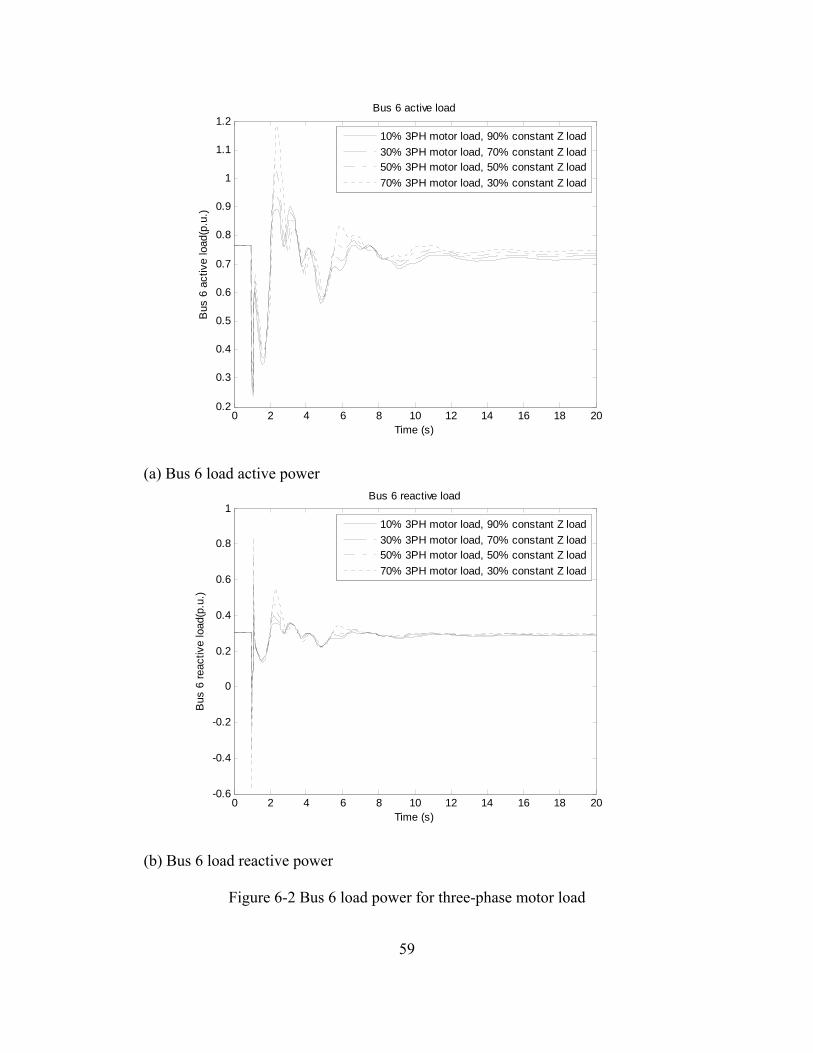
Simulation results of the four load cases are shown in Figure 6-2. After the
fault is cleared, the active loads oscillate and slowly returned to a stable state. The
reactive load power shows spikes when the fault occurs and when it is cleared. By
the end of this 20 seconds simulation, the loads in the four test cases are slightly
different because the amount of actual motor load is affected by power flow
calculation in the post-fault transmission network.
59
(a) Bus 6 load active power
(b) Bus 6 load reactive power
Figure 6-2 Bus 6 load power for three-phase motor load
0 2 4 6 8 10 12 14 16 18 200.2
0.3
0.4
0.5
0.6
0.7
0.8
0.9
1
1.1
1.2
Time (s)
Bus 6 active load
Bus
6 a
ctiv
e lo
ad(p
.u.)
10% 3PH motor load, 90% constant Z load
30% 3PH motor load, 70% constant Z load50% 3PH motor load, 50% constant Z load
70% 3PH motor load, 30% constant Z load
0 2 4 6 8 10 12 14 16 18 20-0.6
-0.4
-0.2
0
0.2
0.4
0.6
0.8
1
Time (s)
Bus 6 reactive load
Bus
6 r
eact
ive
load
(p.u
.)
10% 3PH motor load, 90% constant Z load
30% 3PH motor load, 70% constant Z load50% 3PH motor load, 50% constant Z load
70% 3PH motor load, 30% constant Z load
60
The voltage magnitude and angles at bus 6 corresponding to different
motor load percentage are shown in Figure 6-3 and Figure 6-4.
Figure 6-3 shows that the voltage in all cases initially recovered to about
90% and then reduced to around 0.65 p.u.. Some ringing can be seen as the
voltage returned to a stable value of 0.98 p.u..
Figure 6-3 Bus 6 voltage magnitude for three-phase motor load
The bus angles presented in Figure 6-4 shows the angle difference
between bus 6 and the swing bus. After the fault, the angle difference spiked then
settled to a new stable value.
0 2 4 6 8 10 12 14 16 18 200.5
0.6
0.7
0.8
0.9
1
1.1
1.2
1.3
Time (s)
Bus 6 voltage
Bus
6 v
olta
ge(p
.u.)
10% 3PH motor load, 90% constant Z load
30% 3PH motor load, 70% constant Z load50% 3PH motor load, 50% constant Z load
70% 3PH motor load, 30% constant Z load
61
Figure 6-4 Bus 6 voltage angle for three-phase motor load
6.3.2 Single-phase motor load
The tests in this section are to investigate the influence of single-phase
motor load on the power system. The distribution system arrangement is shown in
Figure 6-1. Four distribution systems were configured with all single-phase
motors but with various percentages. The four load cases are summarized in Table
6.2. The equipment-level model for single-phase induction machine is based on
the phasor model of Section Error! Reference source not found.. Furthermore
different protection switch setups were configured for each load case for a total of
eight variations of load on bus 6.
0 2 4 6 8 10 12 14 16 18 20-0.2
-0.15
-0.1
-0.05
0
0.05
0.1
0.15
0.2
0.25
0.3
Time (s)
Bus 6 voltage anlge
Bus
6 v
olta
ge a
ngle
(rad
)
10% 3PH motor load, 90% constant Z load
30% 3PH motor load, 70% constant Z load50% 3PH motor load, 50% constant Z load
70% 3PH motor load, 30% constant Z load
62
Table 6.2 Distribution systems with single-phase motor load
Case number
Constant Z load (%)
Motor load (%)
Motor type Number of
motors
1 90 10 Single -phase
720
2 70 30 Single -phase
2160
3 50 50 Single -phase
3600
4 30 70 Single -phase
5040
6.3.2.1 Protection switch setup
To represent an actual RAC, TOL and UVL protection logic was included
in the phasor model. Two protection switch configurations are defined in this
research to represent extreme settings:
Protection switch setup 1: The TOL open time set is longer that the
simulation time, thus disabling TOL protection. The UVL threshold is
set at a very low level of 0.4 p.u..
Protection switch setup 2: The TOL switch of the RAC disconnects
the RAC from the grid after a stall of 5 seconds or longer. The UVL
threshold is set at 0.52 p.u..
6.3.2.2 Simulation results with protection switch setup 1
The load power on bus 6 is shown in Figure 6-5. The real and reactive
power draw significantly increases for the 50% motor load case. This is because
the single-phase motors in the distribution system stalled and thus consumed more
power than normal operation. The reactive power increase is much more than the
63
active power due to the low power factor of RAC motors under stall condition.
(a) Bus 6 load active power
(b) Bus 6 load reactive power
Figure 6-5 Bus 6 load power with protection setup 1
0 2 4 6 8 10 12 14 16 18 200.1
0.2
0.3
0.4
0.5
0.6
0.7
0.8
0.9
1
1.1
Time (s)
Bus 6 active load
Bus
6 a
ctiv
e lo
ad(p
.u.)
10% 1PH motor load, 90% constant Z load
30% 1PH motor load, 70% constant Z load50% 1PH motor load, 50% constant Z load
70% 1PH motor load, 30% constant Z load
0 2 4 6 8 10 12 14 16 18 200
0.2
0.4
0.6
0.8
1
1.2
1.4
Time (s)
Bus 6 reactive load
Bus
6 r
eact
ive
load
(p.u
.)
10% 1PH motor load, 90% constant Z load
30% 1PH motor load, 70% constant Z load50% 1PH motor load, 50% constant Z load
70% 1PH motor load, 30% constant Z load
64
Since motor load of the 70% case was removed at 1.9158 seconds by UVL
protection, the total load reduced significantly.
The voltages magnitude and angle at bus 6 are shown in Figure 6-6 and
Figure 6-7 respectively. The voltage magnitude and angle in all test cases reached
a stable level after the fault.
Figure 6-6 Bus 6 voltage magnitude with protection setup 1
0 2 4 6 8 10 12 14 16 18 200.4
0.5
0.6
0.7
0.8
0.9
1
1.1
1.2
1.3
Time (s)
Bus 6 voltage
Bus
6 v
olta
ge(p
.u.)
10% 1PH motor load, 90% constant Z load
30% 1PH motor load, 70% constant Z load50% 1PH motor load, 50% constant Z load
70% 1PH motor load, 30% constant Z load
65
Figure 6-7 Bus 6 voltage angle with protection setup 1
In case that all the RAC motors included in the power system are equipped
with protection setup 1, simulation results shows that:
For 10 % motor load, the motor speed was almost constant during the
entire simulation.
For the 30% single-phase motor load, the speed reduced a little during
the fault but recovered shortly after it was cleared.
For the 50% single-phase motor case, the motors stalled at 2.005
seconds.
For the 70% single-phase motor load case, the under-voltage contact
switch opened at 1.9158 seconds
6.3.2.3 Simulation results with protection switch setup 2
The power at bus 6 during the simulation is shown in Figure 6-8.
0 2 4 6 8 10 12 14 16 18 20-0.4
-0.3
-0.2
-0.1
0
0.1
0.2
0.3
Time (s)
Bus 6 voltage anlge
Bus
6 v
olta
ge a
ngle
(rad
)
10% 1PH motor load, 90% constant Z load
30% 1PH motor load, 70% constant Z load50% 1PH motor load, 50% constant Z load
70% 1PH motor load, 30% constant Z load
66
(a) Bus 6 load active power
(b) Bus 6 load reactive power
Figure 6-8 Bus 6 load power with protection setup 2
0 2 4 6 8 10 12 14 16 18 200.1
0.2
0.3
0.4
0.5
0.6
0.7
0.8
0.9
1
1.1
Time (s)
Bus 6 active load
Bus
6 a
ctiv
e lo
ad(p
.u.)
10% 1PH motor load, 90% constant Z load
30% 1PH motor load, 70% constant Z load50% 1PH motor load, 50% constant Z load
70% 1PH motor load, 30% constant Z load
0 2 4 6 8 10 12 14 16 18 200
0.2
0.4
0.6
0.8
1
1.2
1.4
Time (s)
Bus 6 reactive load
Bus
6 r
eact
ive
load
(p.u
.)
10% 1PH motor load, 90% constant Z load
30% 1PH motor load, 70% constant Z load50% 1PH motor load, 50% constant Z load
70% 1PH motor load, 30% constant Z load
67
Since the stalled motors of the 50% single-phase motor load case consume much
more power, the TOL switch removed the entire single-phase motor load at about 7
s. Load shedding can also be seen for the 70% single-phase motor load case.
Figure 6-9 shows after the fault was cleared, the bus voltage drop of the 50%
case is much lower than other 3 test cases. This is due to the high power demand
of the stalled machines. After the motors are disconnected, the voltage recovers.
Figure 6-9 Bus 6 voltage magnitude with protection setup 2
The bus angles presented in Figure 6-10 show that power system is able to
keep the rotor angle stable with the protection switch setup 2.
0 2 4 6 8 10 12 14 16 18 200.5
0.6
0.7
0.8
0.9
1
1.1
1.2
1.3
Time (s)
Bus 6 voltage
Bus
6 v
olta
ge(p
.u.)
10% 1PH motor load, 90% constant Z load
30% 1PH motor load, 70% constant Z load50% 1PH motor load, 50% constant Z load
70% 1PH motor load, 30% constant Z load
68
Figure 6-10 Bus 6 voltage angle with protection setup 2
In the case that all RAC motors are equipped with the protection switch
setup 2, results indicate:
For the 10% single-phase motor load, neither protection mechanisms
activated.
Also for the 30% motor load case neither protection mechanisms
activated.
For the 50% motor load case the UVL switch did not open but the
motor stalled at 2.005 s thus triggering the TOL switch 5 seconds later.
For the 70% single-phase motor load, the UVL protection switch
opened at 1.0395 s.
6.4 Case analysis
Simulation results from the previous section are now compared in a
0 2 4 6 8 10 12 14 16 18 20-0.35
-0.3
-0.25
-0.2
-0.15
-0.1
-0.05
0
0.05
0.1
0.15
Time (s)
Bus 6 voltage anlge
Bus
6 v
olta
ge a
ngle
(rad
)
10% 1PH motor load, 90% constant Z load
30% 1PH motor load, 70% constant Z load50% 1PH motor load, 50% constant Z load
70% 1PH motor load, 30% constant Z load
69
different manner. Single phase and the equivalent three phase simulation results
are compared for a given percentage of motor load penetration. Table 6.3 shows
the various comparison sets.
Table 6.3 Comparison sets for different motor load percentage
Comparison set Motor type Protection switch setup
10% motor load
Three-phase None
Single-phase Setup 1
Single-phase Setup 2
30% motor load
Three-phase None
Single-phase Setup 1
Single-phase Setup 2
50% motor load
Three-phase None
Single-phase Setup 1
Single-phase Protection switch setup
2
70% motor load
Three-phase None
Single-phase Protection switch setup
1
Single-phase Protection switch setup
2
6.4.1 10% motor load
Figure 6-11 shows the bus apparent power and Figure 6-12 shows the bus
voltage magnitude. It can be seen in Figure 6-11 that after the fault, the apparent
power in the three and single-phase motor load cases have a slight difference.
This is because of changes in power flow in the post-fault transmission network.
The apparent power of the 10% single-phase motor load with switch setups 1 and
2 are the same because no switches opened in both cases. The voltage magnitudes
70
in all the 10% cases are essentially identical.
Figure 6-11 Bus 6 load apparent power for 10% motor load
Figure 6-12 Bus 6 voltage magnitude for 10% motor load
0 2 4 6 8 10 12 14 16 18 200
0.2
0.4
0.6
0.8
1
1.2
1.4
1.6
Time (s)
Bus 6 apparent load
Bus
6 a
ppar
ent
load
(p.u
.)
10% 3PH motor load
10% 1PH motor load with switch setup 110% 1PH motor load with switch setup 2
0 2 4 6 8 10 12 14 16 18 200.5
0.6
0.7
0.8
0.9
1
1.1
1.2
1.3
Time (s)
Bus 6 voltage
Bus
6 v
olta
ge(p
.u.)
10% 3PH motor load
10% 1PH motor load with switch setup 110% 1PH motor load with switch setup 2
71
6.4.2 30% motor load
Figure 6-13 shows the load bus apparent power and Figure 6-14 shows the
load bus voltage magnitude for 30% motor load case. The apparent power of the
30% single-phase motor load with switch setups 1 and 2 are the same because no
switches opened in both cases. The voltage magnitudes in all 30% motor load test
cases nearly match each other.
Figure 6-13 Bus 6 load for 30% motor load
0 2 4 6 8 10 12 14 16 18 200.2
0.3
0.4
0.5
0.6
0.7
0.8
0.9
1
1.1
1.2
Time (s)
Bus 6 apparent load
Bus
6 a
ppar
ent
load
(p.u
.)
30% 3PH motor load
30% 1PH motor load with switch setup 130% 1PH motor load with switch setup 2
72
Figure 6-14 Bus 6 voltage magnitude for 30% motor load
6.4.3 50% motor load
Figure 6-15 shows the bus apparent power for the 50% motor load case.
The TOL switch opened at 7.005 s for the single-phase motor load with switch
setup 2. This removed the motors load from the distribution network. Differences
can be noted between the single phase motor models and equivalent three phase
motor approximation.
0 2 4 6 8 10 12 14 16 18 200.5
0.6
0.7
0.8
0.9
1
1.1
1.2
1.3
Time (s)
Bus 6 voltage
Bus
6 v
olta
ge(p
.u.)
30% 3PH motor load
30% 1PH motor load with switch setup 130% 1PH motor load with switch setup 2
73
Figure 6-15 Bus 6 load for 50% motor load
Figure 6-16 shows the bus voltage magnitude for 50% motor load case.
With switch setup 2, the voltage increases after the TOL switch opens at 7.005 s.
Since the TOL switch did not open in 50% case with switch setup 1, the high
power demand pulled the voltage down. These two 50% single-phase motor cases
illustrate FIDVR. Again it can be seen that the three phase aggregate
approximation is not sufficiently accurate for this type of voltage stability study.
0 2 4 6 8 10 12 14 16 18 200.2
0.4
0.6
0.8
1
1.2
1.4
1.6
1.8
Time (s)
Bus 6 apparent load
Bus
6 a
ppar
ent
load
(p.u
.)
50% 3PH motor load
50% 1PH motor load with switch setup 150% 1PH motor load with switch setup 2
74
Figure 6-16 Bus 6 voltage magnitude for 50% motor load
6.4.4 70% motor load
Figure 6-17 shows the bus apparent power and Figure 6-18 shows the bus
voltage magnitude for 70 % motor load case. The three-phase motor load
recovered but the single-phase motor loads were removed soon after the fault,
both from UVL protection. The single phase motor load with protection setup 2
(.4 p.u. UVL threshold) experienced a deep voltage drop. Both single phase motor
load cases experienced greater voltage sag than the equivalent three phase case.
0 2 4 6 8 10 12 14 16 18 200.5
0.6
0.7
0.8
0.9
1
1.1
1.2
1.3
Time (s)
Bus 6 voltage
Bus
6 v
olta
ge(p
.u.)
50% 3PH motor load
50% 1PH motor load with switch setup 150% 1PH motor load with switch setup 2
75
Figure 6-17 Bus 6 load for 70% motor load
Figure 6-18 Bus 6 voltage magnitude for 70% motor load
0 2 4 6 8 10 12 14 16 18 200
0.2
0.4
0.6
0.8
1
1.2
1.4
Time (s)
Bus 6 apparent load
Bus
6 a
ppar
ent
load
(p.u
.)
70% 3PH motor load
70% 1PH motor load with switch setup 170% 1PH motor load with switch setup 2
0 2 4 6 8 10 12 14 16 18 200.4
0.5
0.6
0.7
0.8
0.9
1
1.1
1.2
1.3
Time (s)
Bus 6 voltage
Bus
6 v
olta
ge(p
.u.)
70% 3PH motor load
70% 1PH motor load with switch setup 170% 1PH motor load with switch setup 2
76
CHAPTER 7
CONCLUSIONS AND FUTURE WORK
7.1 Conclusions
In this work simulation of fault induced delayed voltage recovery was
investigated. The focus was primarily on load representation of residential air
conditioners in simulation.
First the topic of voltage stability was categorized. Static and dynamic
simulation methods were discussed in context of voltage stability. Voltage
stability indices were categorized. The FIDVR voltage stability phenomenon was
defined and a brief literature review of various FIDVR events was presented. Also
some FIDVR solutions were listed.
Static load, dynamic load, and composite load modeling and associated
parameter extraction methods were presented. Common dynamic models for
single and three phase induction machines were listed.
Properties of typical RACs were then discussed. Stalling, protection
circuitry, and restarting characteristics of RACs were presented. Past work on
modeling of RACs in context of FIDVR was reviewed. Equipment level and grid
level modeling methods were discussed. The phasor model was presented as a
good equipment level model of RACs. Example three and single phase motor
models were tested for voltage sag characteristics in simulation.
A method was proposed to include detailed single phase load information
in a larger power system simulation to investigate the influence of motor load on
power system stability. An interface method for linking transmission network and
77
detailed distribution network in simulation was presented. The method entails
passing data back and forth each time step.
A transmission network and several detailed distribution systems were
built with different percentage motor load. Each single-phase motor in the
distribution system was represented by the equipment-level phasor model, whose
parameters were collected from a typical RAC compressor unit. Three-phase
aggregate representations of RACs were also built in simulation with different
percentage of motor load.
Simulations were conducted using the new interface method. A fault was
set and cleared in an attempt to induce FIDVR. When the motor loads were
represented by the three phase aggregate representation, no FIDVR events
occurred. The same experiment was conducted with the detailed single phase
models to represent the RACs. FIDVR was reproduced at 50 % motor load.
It can be concluded that the fault induced voltage sag in the distribution
system becomes more severe with the increased single-phase motor load
percentage. In these simulation experiments, the three-phase motor is able to
represent the aggregation effect of the single-phase motor load only when the
motor load percentage is 10% or 30%.
78
7.2 Future work
This work may be extended in a variety of directions. First more
contingencies may be applied, such as unbalanced fault, generator outage, and
increased system load. Also several more distribution systems with
equipment-level models may be included to apply this new method to a larger
area of the power system. A new grid-level single-phase motor model may be
developed based on the findings from simulation results with a variety of
contingencies. This new load model may provide a more accurate grid-level
model representing the aggregating effect of the single-phase motor load.
79
REFERENCES
[1] Prabha Kundur, Power system stability and control, New York: McGraw-Hill, 1994.
[2] P. Kundur et al., “Overview on definition and classification of power system stability,” in CIGRE/IEEE PES Int. Symp. on Quality and Security of Electric Power Delivery Systems, 2003, pp. 1-4.
[3] C. W. Taylor, Power system voltage stability, New York: McGraw-Hill, 1994.
[4] Appliance report on US households. [Online]. Available: http://www.eia.doe.gov/emeu/reps/appli/all_tables.html
[5] IEEE/PES power system stability subcommittee special publication, Voltage stability assessment: concepts, practices and tools, Aug., 2002.
[6] J. D. Glover and M. S. Sarma, Power System Analysis and Design, Boston: PWS Pub., 1994.
[7] L. M. C. Braz et al., “A critical evaluation of step size optimization based load flow methods,” IEEE Trans. Power Syst., vol. 15, no. 1, pp. 202-207, Feb. 2000.
[8] A. Wiszniewski, “New Criteria of Voltage Stability Margin for the Purpose of Load Shedding,” IEEE Trans. Power Del., vol. 22, no. 3, pp.1367-1371, Jul. 2007.
[9] G. K. Morison et al., “Voltage stability analysis using static and dynamic approaches,” IEEE Trans. Power Syst., vol.8, no. 3, pp. 1159-1171, Aug. 1993.
[10] B. Delfino et al., “Voltage stability of power systems: Links between static and dynamic approaches,” Electrotechnical Conference, Bari, Italy, 1996, vol. 2, pp. 854-858.
[11] M. Hasani and M. Parniani, “Method of combined static and dynamic analysis of voltage collapse in voltage stability assessment,” IEEE/PES Transmission and Distribution Conf. and Exhibition: Asia and Pacific, 2005, pp.1-6.
[12] IEEE special publication 90TH0358-2-PWR, Voltage stability of power systems: concepts, analytical tools, and industry experience, 1990.
80
[13] I. Dobson, “An Iterative method to compute a closest saddle node or hope bifurcation instability in multidimensional parameter space,” 1992 IEEE International Symposium on Circuits and Systems, ISCAS '92. Proceedings, v. 5, pp. 2513 – 2516, 3-6 May 1992.
[14] N. Flatabo et al., “Voltage stability condition in a power transmission system calculated by sensitivity methods,” IEEE Trans. Power Syst., vol. 5, no. 4, pp. 1286-1293, Nov. 1990.
[15] C. Lemaitre et al., “An indicator of the risk of voltage profile instability for real-time control applications,” IEEE Trans. Power Syst., vol. 5, no. 1, pp. 154-161, 1990.
[16] B. Gao et al., “Voltage stability evaluation using modal analysis,” IEEE Trans. Power Syst., vol. 7, no. 4, pp. 1529-1542, Nov. 1992.
[17] P. A. Lof et al., “Fast calculation of a voltage stability index,” IEEE Trans. Power Syst., vol. 7, no. 1, pp. 54-64, Feb. 1992.
[18] Voltage stability analysis program application guide, EPRI project RP3040-1, prepared by Ontario Hydro, October 1992.
[19] C. A. Canizares et al., “Comparison of performance indices for detection of proximity to voltage collapse,” IEEE Trans. Power Syst., vol. 11, no. 3, pp. 1441-1450, Aug. 1996.
[20] A. Tiranuchit et al., “Towards a computationally feasible on-line voltage instability index,” IEEE Trans. Power Syst., vol. 3, no. 2, pp.669-675, May 1988.
[21] A. Tiranuchit and R. J. Thomas, “A posturing strategy against voltage instabilities in electric power systems,” IEEE Trans. Power Syst., vol. 3, no. 1, pp. 87-93, Feb. 1988.
[22] H. Suzuki, “Study group 37 discussions, in Proc. CIGRE 34th Session, vol. 2, pp. 87-93, Feb. 1992.
[23] Y. Tamura et al., “Voltage instability proximity index (VIPI) based on multiple load flow solutions in ill-conditioned power systems,” in Proc. 27th IEEE Conf. on Decision and Control, vol. 3, pp. 2114-2119, Dec. 1988.
[24] J. Hasimoto et al., “On the continuous monitoring of voltage stability margin in electric power systems,” Institute of Electrical Engineers of Japan Transaction, vol. 108-B, no. 2, pp. 65-72, Feb. 1988. (In Japanese)
81
[25] A. Takehara et al., “Voltage stability preventive and emergency-preventive control using VIPI sensitivity,” Electrical Engineering in Japan, vol. 143, no. 4, pp. 22-30, Jun. 2003.
[26] P. Kessel and H. Glavitsch, “Estimating the voltage stability of a power system,” IEEE Trans. Power Del., vol. 1, no. 3, Jul. 1986.
[27] T. Nagao, et al., “Development of static and simulation programs for voltage stability studies of bulk power system,”, IEEE transactions on power systems, v. 12, Issue 1, pp. 273 – 281, Feb. 1997.
[28] “Suggested techniques for voltage stability analysis,” Technical report 93TH0620-5PWR, IEEE/PES, 1993.
[29] NERC Transmission Issues Subcommittee and System Protection and Control Subcommittee, “A Technical Reference Paper Fault-Induced Delayed Voltage Recovery,” Version 1.2, Jun. 2009.
[30] B.R. Williams et al., “Transmission voltage recovery delayed by stalled air-conditioner compressors,” IEEE Trans. Power Syst., vol. 7, no. 3, pp. 1173-1181, Aug. 1992.
[31] J.W. Shaffer, “Air conditioner response to transmission faults,” IEEE Trans. Power Syst., vol. 12, no. 2, pp. 614-621, May 1997.
[32] L. Taylor and S.M. Hsu, “Transmission voltage recovery following a fault event in the metro Atlanta area,” 2000 IEEE PES Summer Meeting, Seattle, WA, vol. 1, pp. 537-542, Jul. 2000.
[33] P. Pourbeik and B. Agrawal, "A hybrid model for representing air-conditioner compressor motor behavior in power system studies," 2008 IEEE PES General Meeting - Conversion and Delivery of Electrical Energy in the 21st Century, Pittsburgh, PA, pp. 1-8, Jul. 2008.
[34] Lawrence Berkeley National Laboratory, “Final project report: load modeling transmission research,” A California Institute for Energy and Environment (CIEE) Report, Mar. 2010.
[35] IEEE Task Force on Load Representation for Dynamic Performance, “Load representation for dynamic performance analysis,” IEEE Trans. Power Syst., vol. 8, no. 2, pp. 472-482, May 1993.
[36] J. Machowski, et al., Power system dynamics: stability and control, 2nd ed., Wiley, 2008.
82
[37] WECC Load Modeling Task Force, Load Modeling for Power System Studies [Online]. Available: http://www.nerc.com/docs/pc/tis/10_Load_Modeling_for_Power_System_Studies.pdf
[38] Leonard L. Grigsby, Electric power generation, transmission, and distribution, 2nd ed., CRC Press, 2007.
[39] W. W. Price, et al., “Load modeling for power flow and transient stability computer studies,” IEEE Trans. Power Systems, vol. 3, no. 1, pp. 180-187, Feb 1988.
[40] G. Karady and K. Holbert, Electrical energy conversion and transport: an interactive computer-based approach, IEEE Computer Society Press, 2004.
[41] M. N. Bandyopadhyay, Electrical Machines: Theory and Practice, Prentice-Hall of India Pvt.Ltd.,Oct. 30, 2008.
[42] N. Mohan, Advanced Electric Drives, Minneapolis. MN: Mnpere, 2001.
[43] D. W. Novotny and T. A. Lipo, Vector Control and Dynamics of AC Drives. New York: Oxford University Press, 1996.
[44] C. M. Trout, Essentials of Electric Motors and Controls, Jones and Bartlett Publishers. LLC, 2010
[45] R. Miller, M. Miller, Industrial Electricity and Motor Controls, McGraw-Hill Inc.,2008
[46] B. Lesieutre et al., “Phasor modeling approach for single phase A/C motors,” 2008 IEEE PES General Meeting, Pittsburgh, PA, pp. 1-7, Jul. 2008.
[47] L. Y. Taylor et al., “Development of load models for fault induced delayed voltage recovery dynamic studies,” 2008 IEEE PES General Meeting - Conversion and Delivery of Electrical Energy in the 21st Century, Pittsburgh, PA , pp. 1 - 7, 20-24 Jul. 2008
[48] W. H. Kersting, Distribution system modeling and analysis, Taylor & Francis Group, LLC., 2007.
[49] A. M. Gaikwad et al., “Results of residential air conditioner testing in WECC,” 2008 IEEE PES General Meeting - Conversion and Delivery of Electrical Energy in the 21st Century, Pittsburgh, PA, pp. 1 – 9, Jul. 2008.
[50] D. Kosterev et al., “Load Modeling in Power System Studies: WECC Progress Update,” 2008 IEEE PES General Meeting - Conversion and Delivery of Electrical Energy in the 21st Century, Pittsburgh, PA, pp. 1-8, Jul. 2008.
83
[51] C. A. Baone et al., “Local voltage support from distributed energy resources to prevent air conditioner motor stalling,” 2010 Innovative Smart Grid Technologies (ISGT), pp. 1-6, 2010.
[52] V. Stewart and E. H. Camm, “Modeling of stalled motor loads for power system short-term voltage stability analysis,” 2005 IEEE PES General Meeting, San Francisco, CA, vol. 2, pp. 1887-1892, Jun. 2005.
[53] PSAT Reference Manual
89
A.1 Coding built in PSAT %Update P, Q, and V_p based on simulation from t0 to DAE.t if T_last < DAE.t SimulinkStartTime=Settings.t0; % End time is increased by 1.5 s,which is the time duration for % 1PH motor to get its normal operation status SimulinkEndTime=DAE.t+1.5; %DAE.y(15)shows the bus 6 voltae magnitude during time-domain %simulation SimulinkVoltage=(DAE.y(15))*Bus.con(6,2)*1000; %DAE.y(6)shows the bus 6 voltae angle in rad during time-domain %simulation SimulinkAngle=DAE.y(6)*180/pi; %DAE.y(1)shows the bus 1 (swing bus) voltae angle in rad during %time-domain simulation Simulink_swing_Angle=DAE.y(1); %Call simulation in distribution network [p_local,q_local,V_p]=Local_simulink_connection(...
SimulinkStartTime,... SimulinkEndTime,SimulinkVoltage,SimulinkAngle,... Simulink_swing_Angle,Simulink_PSAT_Step); T_last=DAE.t;
%Update the P, Q, and V value of transmission load bus based on %simulation in Simulink
%Update the bus 6 voltage DAE.y(15)=V_p; %Update the bus 6 load, if the applied load is out of acceptable %range, the applied load will be multiply with a factor to insure %the actural load applied on the bus 6 is the power needed by the %distribution network if DAE.y(15)<PQ.con(1,7) PQ.con(1,4)=p_local*DAE.y(15)^2/PQ.con(1,7)^2; PQ.con(1,5)=q_local*DAE.y(15)^2/PQ.con(1,7)^2; elseif DAE.y(15)>PQ.con(1,6) PQ.con(1,4)=p_local*DAE.y(15)^2/PQ.con(1,6)^2; PQ.con(1,5)=q_local*DAE.y(15)^2/PQ.con(1,6)^2; else PQ.con(1,4)=p_local; PQ.con(1,5)=q_local; end %$$$$$$$$$$$$$$$$$$$$$$$$$$$$$$$$$$$$$$$$$$$$$$$$$$$$$$$$$$$$$$$$$$$$$$ end
A.2 Coding for time-domain power flow analysis in Simulink
function[p_local,q_local,V_p]=Local_simulink_connection(... SimulinkStartTime,SimulinkEndTime,SimulinkVoltage,... SimulinkAngle,Simulink_swing_Angle,Simulink_PSAT_Step) %Record the system data during the entire simulation in Simulink global Db_S_1 Db_S_2A Db_S_2B Db_S_2C Db_S_3_230 Db_S_3_69 %Record the simulation initial and final stage global Simul_stage_1 Simul_stage_2A Simul_stage_2B
90
global Simul_stage_2C Simul_stage_3 %Record exchange data between simulink and psat. global Simulink_PSAT_Step % Record the start and end time of simulation global SimulinkStartTime SimulinkEndTime %For parameters of RAC motor global V_freq W_s W_b R_ds R_qs X_r X_c X_ds X_qs X_m H n global A_sat b_sat T_o f_base V_base P_base I_base Z_base T_base global X1 X2A X2B X2C X3 global IN_V V_angle global V_12_Step1_R Total_12_A_R Total_12_B_R Total_12_C_R global Db_last V_last P_last Q_last %Update the input voltage of distribution system with bus 6 voltage vector IN_V=SimulinkVoltage; V_angle=SimulinkAngle; %Perform simulation step 1, get the voltage applied on the motor [Data_row_last,Data_col_last]=size(Db_S_1); open_system('HV_local_21_Step_1.mdl') hAcs = getActiveConfigSet(gcs); hAcs.set_param('StartTime', 'SimulinkStartTime'); hAcs.set_param('StopTime', 'SimulinkEndTime'); hAcs.set_param('LoadInitialState','on'); simOut = sim('HV_local_21_Step_1.mdl'); %%%%%% V_12_Step1_R=V_12_Step1; [P_row,P_col]=size(V_12_Step1.time); for row=1:P_row Db_S_1(row+Data_row_last,1)=V_12_Step1.time(row,1); Db_S_1(row+Data_row_last,2)=V_12_Step1.signals.values(row,1); Db_S_1(row+Data_row_last,3)=V_12_Step1.signals.values(row,2); Db_S_1(row+Data_row_last,4)=V_12_Step1.signals.values(row,3); end %Base on applied voltage, calculate the motor response in each phase %Perform simulation step 2 for Phase A [Data_row_last,Data_col_last]=size(Db_S_2A); open_system('HV_local_21_Step_2_A.mdl') hAcs = getActiveConfigSet(gcs); hAcs.set_param('StartTime', 'SimulinkStartTime'); hAcs.set_param('StopTime', 'SimulinkEndTime'); hAcs.set_param('LoadInitialState','on'); simOut = sim('HV_local_21_Step_2_A.mdl'); %%%%%% Total_12_A_R=Total_12_A; [P_row,P_col]=size(Motor_240_A.time); for row=1:P_row Db_S_2A(row+Data_row_last,1)=Motor_240_A.time(row,1); Db_S_2A(row+Data_row_last,2)=Motor_240_A.signals.values(row,1); Db_S_2A(row+Data_row_last,3)=Motor_240_A.signals.values(row,2); Db_S_2A(row+Data_row_last,4)=Motor_240_A.signals.values(row,3); Db_S_2A(row+Data_row_last,5)=Motor_240_A.signals.values(row,4); Db_S_2A(row+Data_row_last,6)=Motor_240_A.signals.values(row,5); Db_S_2A(row+Data_row_last,7)=Motor_240_A.signals.values(row,6); Db_S_2A(row+Data_row_last,8)=Motor_240_A.signals.values(row,7);
91
Db_S_2A(row+Data_row_last,9)=Motor_240_A.signals.values(row,8); Db_S_2A(row+Data_row_last,10)=Motor_240_A.signals.values(row,9); Db_S_2A(row+Data_row_last,11)=Motor_240_A.signals.values(row,10); Db_S_2A(row+Data_row_last,12)=Total_240_A.signals.values(row,1); Db_S_2A(row+Data_row_last,13)=Total_240_A.signals.values(row,2); Db_S_2A(row+Data_row_last,14)=Total_240_A.signals.values(row,3); Db_S_2A(row+Data_row_last,15)=Total_240_A.signals.values(row,4); Db_S_2A(row+Data_row_last,16)=Total_12_A.signals.values(row,1); Db_S_2A(row+Data_row_last,17)=Total_12_A.signals.values(row,2); Db_S_2A(row+Data_row_last,18)=Total_12_A.signals.values(row,3); Db_S_2A(row+Data_row_last,19)=Total_12_A.signals.values(row,4);
end %Perform simulation step 2 for Phase B [Data_row_last,Data_col_last]=size(Db_S_2B); open_system('HV_local_21_Step_2_B.mdl') hAcs = getActiveConfigSet(gcs); hAcs.set_param('StartTime', 'SimulinkStartTime'); hAcs.set_param('StopTime', 'SimulinkEndTime'); hAcs.set_param('LoadInitialState','on'); simOut = sim('HV_local_21_Step_2_B.mdl'); %%%%%% Total_12_B_R=Total_12_B; [P_row,P_col]=size(Motor_240_B.time); for row=1:P_row Db_S_2B(row+Data_row_last,1)=Motor_240_B.time(row,1); Db_S_2B(row+Data_row_last,2)=Motor_240_B.signals.values(row,1); Db_S_2B(row+Data_row_last,3)=Motor_240_B.signals.values(row,2); Db_S_2B(row+Data_row_last,4)=Motor_240_B.signals.values(row,3); Db_S_2B(row+Data_row_last,5)=Motor_240_B.signals.values(row,4); Db_S_2B(row+Data_row_last,6)=Motor_240_B.signals.values(row,5); Db_S_2B(row+Data_row_last,7)=Motor_240_B.signals.values(row,6); Db_S_2B(row+Data_row_last,8)=Motor_240_B.signals.values(row,7); Db_S_2B(row+Data_row_last,9)=Motor_240_B.signals.values(row,8); Db_S_2B(row+Data_row_last,10)=Motor_240_B.signals.values(row,9); Db_S_2B(row+Data_row_last,11)=Motor_240_B.signals.values(row,10); Db_S_2B(row+Data_row_last,12)=Total_240_B.signals.values(row,1); Db_S_2B(row+Data_row_last,13)=Total_240_B.signals.values(row,2); Db_S_2B(row+Data_row_last,14)=Total_240_B.signals.values(row,3); Db_S_2B(row+Data_row_last,15)=Total_240_B.signals.values(row,4); Db_S_2B(row+Data_row_last,16)=Total_12_B.signals.values(row,1); Db_S_2B(row+Data_row_last,17)=Total_12_B.signals.values(row,2); Db_S_2B(row+Data_row_last,18)=Total_12_B.signals.values(row,3); Db_S_2B(row+Data_row_last,19)=Total_12_B.signals.values(row,4);
end %Perform simulation step 2 for Phase C [Data_row_last,Data_col_last]=size(Db_S_2C); open_system('HV_local_21_Step_2_C.mdl') hAcs = getActiveConfigSet(gcs); hAcs.set_param('StartTime', 'SimulinkStartTime'); hAcs.set_param('StopTime', 'SimulinkEndTime'); hAcs.set_param('LoadInitialState','on');
92
simOut = sim('HV_local_21_Step_2_C.mdl'); %%%%%% Total_12_C_R=Total_12_C; [P_row,P_col]=size(Motor_240_C.time); for row=1:P_row Db_S_2C(row+Data_row_last,1)=Motor_240_C.time(row,1); Db_S_2C(row+Data_row_last,2)=Motor_240_C.signals.values(row,1); Db_S_2C(row+Data_row_last,3)=Motor_240_C.signals.values(row,2); Db_S_2C(row+Data_row_last,4)=Motor_240_C.signals.values(row,3); Db_S_2C(row+Data_row_last,5)=Motor_240_C.signals.values(row,4); Db_S_2C(row+Data_row_last,6)=Motor_240_C.signals.values(row,5); Db_S_2C(row+Data_row_last,7)=Motor_240_C.signals.values(row,6); Db_S_2C(row+Data_row_last,8)=Motor_240_C.signals.values(row,7); Db_S_2C(row+Data_row_last,9)=Motor_240_C.signals.values(row,8); Db_S_2C(row+Data_row_last,10)=Motor_240_C.signals.values(row,9); Db_S_2C(row+Data_row_last,11)=Motor_240_C.signals.values(row,10); Db_S_2C(row+Data_row_last,12)=Total_240_C.signals.values(row,1); Db_S_2C(row+Data_row_last,13)=Total_240_C.signals.values(row,2); Db_S_2C(row+Data_row_last,14)=Total_240_C.signals.values(row,3); Db_S_2C(row+Data_row_last,15)=Total_240_C.signals.values(row,4); Db_S_2C(row+Data_row_last,16)=Total_12_C.signals.values(row,1); Db_S_2C(row+Data_row_last,17)=Total_12_C.signals.values(row,2); Db_S_2C(row+Data_row_last,18)=Total_12_C.signals.values(row,3); Db_S_2C(row+Data_row_last,19)=Total_12_C.signals.values(row,4);
end %Perform simulation step 3 and calculate the latest P,Q, and V_P [Data_row_last,Data_col_last]=size(Db_S_3_230); open_system('HV_local_21_Step_3.mdl') hAcs = getActiveConfigSet(gcs); hAcs.set_param('StartTime', 'SimulinkStartTime'); hAcs.set_param('StopTime', 'SimulinkEndTime'); hAcs.set_param('LoadInitialState','on'); simOut = sim('HV_local_21_Step_3.mdl'); %Find load and V+ [P_row P_Col]=size(Total_230.signals.values); for row=1:P_row Db_S_3_230(row+Data_row_last,1)=Total_230.time(row,1); Db_S_3_230(row+Data_row_last,2)=Total_230.signals.values(row,1); Db_S_3_230(row+Data_row_last,3)=Total_230.signals.values(row,2); Db_S_3_230(row+Data_row_last,4)=Total_230.signals.values(row,3); Db_S_3_230(row+Data_row_last,5)=Total_230.signals.values(row,4); Db_S_3_230(row+Data_row_last,6)=Total_230.signals.values(row,5); Db_S_3_230(row+Data_row_last,7)=Total_230.signals.values(row,6); Db_S_3_230(row+Data_row_last,8)=Total_230.signals.values(row,7); Db_S_3_230(row+Data_row_last,9)=Total_230.signals.values(row,8); Db_S_3_230(row+Data_row_last,10)=Total_230.signals.values(row,9); Db_S_3_230(row+Data_row_last,11)=Total_230.signals.values(row,10); Db_S_3_230(row+Data_row_last,12)=Total_230.signals.values(row,11); Db_S_3_230(row+Data_row_last,13)=Total_230.signals.values(row,12);
93
Db_S_3_230(row+Data_row_last,14)=Total_230.signals.values(row,13); Db_S_3_230(row+Data_row_last,15)=Total_230.signals.values(row,14); Db_S_3_230(row+Data_row_last,16)=Total_230.signals.values(row,15);
end for row=1:P_row Db_S_3_69(row+Data_row_last,1)=Total_69.time(row,1); Db_S_3_69(row+Data_row_last,2)=Total_69.signals.values(row,1); Db_S_3_69(row+Data_row_last,3)=Total_69.signals.values(row,2); Db_S_3_69(row+Data_row_last,4)=Total_69.signals.values(row,3); Db_S_3_69(row+Data_row_last,5)=Total_69.signals.values(row,4); Db_S_3_69(row+Data_row_last,6)=Total_69.signals.values(row,5); Db_S_3_69(row+Data_row_last,7)=Total_69.signals.values(row,6); Db_S_3_69(row+Data_row_last,8)=Total_69.signals.values(row,7); Db_S_3_69(row+Data_row_last,9)=Total_69.signals.values(row,8); Db_S_3_69(row+Data_row_last,10)=Total_69.signals.values(row,9); Db_S_3_69(row+Data_row_last,11)=Total_69.signals.values(row,10); Db_S_3_69(row+Data_row_last,12)=Total_69.signals.values(row,11); Db_S_3_69(row+Data_row_last,13)=Total_69.signals.values(row,12); Db_S_3_69(row+Data_row_last,14)=Total_69.signals.values(row,13); Db_S_3_69(row+Data_row_last,15)=Total_69.signals.values(row,14); Db_S_3_69(row+Data_row_last,16)=Total_69.signals.values(row,15);
end %%%%%%%%%%%%%%%%%%%%%%%%%%%%%%%%%%%%%%%%%%%%%%%%%%%%%%%%%%%%%%%%% %Find the latest P,Q, and V_P and return these value to the function [Data_row_last,Data_col_last]=size(Db_S_3_230); V_p_230=Db_S_3_230(Data_row_last,2); P_230=Db_S_3_230(Data_row_last,3); Q_230=Db_S_3_230(Data_row_last,4); %If positive sequence of supply voltage in distribution system is more %than input voltage, then update the transmission load bus voltage if V_p_230 > SimulinkVoltage V_p=V_p_230/230000; else V_p=SimulinkVoltage/230000; end %Assume there are two same local netowork p_local=2*P_230/1e8; q_local=2*Q_230/1e8; %Write data to Simulink_PSAT_Step [Simu_row,Simu_col]=size(Simulink_PSAT_Step); Simulink_PSAT_Step(Simu_row+1,1)=SimulinkStartTime;%s Simulink_PSAT_Step(Simu_row+1,2)=SimulinkEndTime-1.5;%s Simulink_PSAT_Step(Simu_row+1,3)=SimulinkVoltage/230000;%p.u. Simulink_PSAT_Step(Simu_row+1,4)=SimulinkAngle*pi/180;%rad Simulink_PSAT_Step(Simu_row+1,5)=Simulink_swing_Angle;%rad Simulink_PSAT_Step(Simu_row+1,6)=V_p;%p.u. Simulink_PSAT_Step(Simu_row+1,7)=p_local;%p.u. Simulink_PSAT_Step(Simu_row+1,8)=q_local;%p.u.