Should we trust graphs' default settings in the R packages?
Agnieszka Wnuk1*, Konrad J. Dębski2
1 Department of Experimental Design and Bioinformatics, Warsaw University of Life Sciences, Nowoursynowska 159, 02-776 Warsaw, Poland. 2 Laboratory of Bioinformatics, Neurobiology Center, Nencki Institute of Experimental Biology, Polish Academy of Sciences, Warsaw, Poland. *Corresponding author: Agnieszka Wnuk; E-mail: [email protected]
CITATION: Wnuk A., Dębski K.J. (2016). Should we trust graphs' default settings in the R packages? Communications in Biometry and Crop Science 11, 114–126.
ABSTRACT Nowadays, we cannot imagine conducting analysis and creating any graph without support of various computer programs. They make researchers’ work easier. No matter how good their computer skills are, it is always nice to have some help, and that is what default settings usually are for. It is believed that using default settings of graphical software, one should not worry about choice of graph settings. But is it actually true? Perhaps researchers are putting too much trust in default settings? In this article, we will try to show that default settings are not always as helpful as it seems. We will demonstrate this with examples of three packages in R: graphics, lattice and ggplot2.
Key Words: default settings; graphs; R environment.
INTRODUCTION
A scientific publication is one of various methods of presenting research results to fellow researchers. Nowadays, any research publication is made using computer resources that helps collect and analyze data, edit and format text, make tables and graphs. As researchers related to data analysis and scientific visualization, we cannot imagine our research without programs such as R, SAS, Statistica, Statgraphics, MATLAB, spreadsheet software (Excel or Calc) etc. Some of these programs are quite simple to use while others require basic or even advanced programming skills. A choice of right software usually depends on our preferences, skills, or purposes of the analysis. These programs have much in common as they all provide a multitude of built-in functions and tools, and each of them has default settings. In many situations, default settings will be useful indeed. In many other situations, however, they can cause problems when one starts trusting them too much: they can mislead us into feeling that we do not have to worry about every detail – because the default settings do it for us.
HTTP://AGROBIOL.SGGW.WAW.PL/CBCS
COMMUNICATIONS IN BIOMETRY AND CROP SCIENCE Vol. 11, NO. 2, 2016, PP. 114–126
INTERNATIONAL JOURNAL OF THE FACULTY OF AGRICULTURE AND BIOLOGY, Warsaw University of Life Sciences – SGGW, POLAND
Wnuk & Dębski – Shou ld we t rust graphs ' defau lt set t ings in the R packages?
115
In this paper, we discuss problems related to default settings of graphs. So far, only a few authors have noticed that default settings of graphs can cause problems (Bergman et al. 1995, Reese 2006, Su 2008, Rougier et al. 2014). Other authors pointed out that the creation of a graph should be a well-thought process (e.g. Tufte 1991, 1997, 2001, Cleveland and McGill 1985, Cleveland 1993, 1994, Yandell 2007, Kozak 2010). In this paper, we focus on R environment (R Core Team 2015), one of the most popular and free tools for data analysis and presentation these days. We will try to show some issues related to default setting of graphs with two simple examples based on a graphical function in R using packages {graphics}, {lattice} and {ggplot2}. However, conclusions obtained here can be easily applied to other functions and computer programs.
Example 1: Default settings of the legend in graphics and lattice packages. Each R function has default settings (parameters), which are used when a function is
called without specifying this parameter. Let the example be the simplest function used to create a scatter plot − plot() in the package {graphics} (R Core Team, 2014):
plot(x, y, ...)
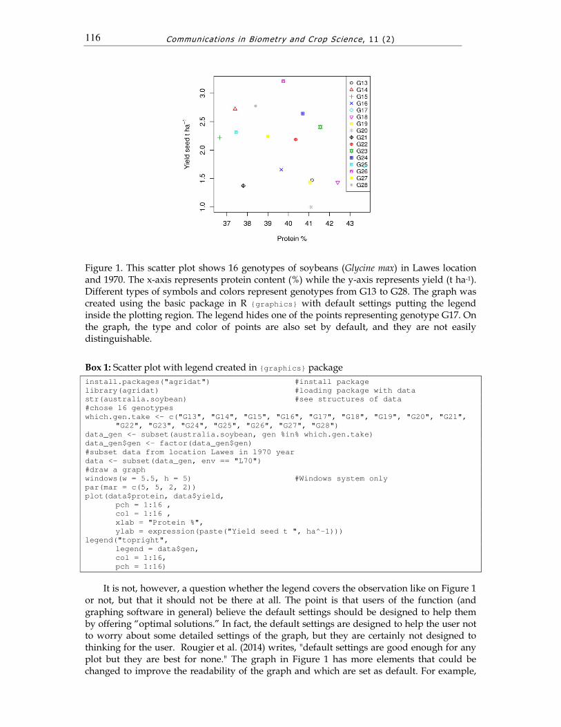
where x, y are coordinates of the points, and (...) are other/optional graphical parameters which are passed to the methods used in the function body and are not listed directly. Depending on the type of the input data, different plot methods are called to handle the input data. For vectors the plot.default() function is called. To create a graph this function required only the data, that is, x, y coordinates for all points. The plot.default() automatically sets graphical parameters of the plot such as type of points, axis scales, label for the x and y axis etc. (for more details see ?plot.default). For this example, we used only a fragment of data from australia.soybean datasets released in the package {agridat} (Wright 2014) and provided by Basford (1982) and Kroonenberg and Basford (1989). Figure 1 presents the relationship between protein content and yield seed for 16 genotypes of soybean (Glycine max) in one location (Lawes) in 1970 year (see Box 1).
A separate function legend () is used to add a legend to the plot (in the package {graphic}). In this function, we do not choose where the legend is placed on the graph region (the whole area that the graph takes). The default location is inside of the plotting region (the area bounded by the axes of the graph), which contains data region (where points are plotted). The legend() requires x and y coordinates or keyword for set position of the legend (all arguments can be found calling up ?legend). Thus it is not possible to put legend outside of the plotting region. In Figure 1, the legend is set in the top right corner of the plot. However, after a more careful look we will see that it covers one of the points, that representing genotype 17 (under the genotype 25). Of course, we want to fix this error immediately, but how exactly are we supposed to do that? The space inside the plotting region is too small to place the legend there because it will always cover the data (Figure 1).
In general, one can say that the default settings of a function are poorly designed when they force the function to do something which is against the principles of a proper construction of the graphs (e.g. Cleveland 1994, pp. 46-49, Kozak 2010). The legend inside the plotting region often interferes with the data, thereby making their analysis more difficult; thus, the usefulness of the graph decreases. According to Cleveland (1994), only data points should be placed in the plotting region. Exceptions to this rule can be specific, important (usually short) information supporting analysis or presenting the data, e.g., a regression line or equation. Unfortunately, the legend is often put inside the plotting region (e.g. Maddonni et al. 2006, Timsina and Humphreys 2006, Lamkey and Lorenz 2014, Melchinger et al. 2015, Morrison et al. 2015).
Communicat ions in Biometry and Crop Sc ience , 11 (2)
116
Figure 1. This scatter plot shows 16 genotypes of soybeans (Glycine max) in Lawes location and 1970. The x-axis represents protein content (%) while the y-axis represents yield (t ha-1). Different types of symbols and colors represent genotypes from G13 to G28. The graph was created using the basic package in R {graphics} with default settings putting the legend inside the plotting region. The legend hides one of the points representing genotype G17. On the graph, the type and color of points are also set by default, and they are not easily distinguishable.
Box 1: Scatter plot with legend created in {graphics} package
data_gen <- subset(australia.soybean, gen %in% which.gen.take)
data_gen$gen <- factor(data_gen$gen)
#subset data from location Lawes in 1970 year
data <- subset(data_gen, env == "L70")
#draw a graph
windows(w = 5.5, h = 5) #Windows system only
par(mar = c(5, 5, 2, 2))
plot(data$protein, data$yield,
pch = 1:16 ,
col = 1:16 ,
xlab = "Protein %",
ylab = expression(paste("Yield seed t ", ha^-1)))
legend("topright",
legend = data$gen,
col = 1:16,
pch = 1:16)
It is not, however, a question whether the legend covers the observation like on Figure 1 or not, but that it should not be there at all. The point is that users of the function (and graphing software in general) believe the default settings should be designed to help them by offering “optimal solutions.” In fact, the default settings are designed to help the user not to worry about some detailed settings of the graph, but they are certainly not designed to thinking for the user. Rougier et al. (2014) writes, "default settings are good enough for any plot but they are best for none." The graph in Figure 1 has more elements that could be changed to improve the readability of the graph and which are set as default. For example,
Wnuk & Dębski – Shou ld we t rust graphs ' defau lt set t ings in the R packages?
117
the types and colors of points used in the graph are less readable than they could be. In Figure 1, it is difficult to distinguish the genotype 19 and 27 because they are marked with similar shape and color of the symbols (yellow squares).
In R environment, various graphical packages are better or worse adapted to the principles of a proper construction of scientific graphs. Yandell (2007) noticed that the choice of a package can enhance or limit our ability to analyze or present data. We absolutely do not claim that the {graphics} package is essentially bad. We can use functions like plot() and legends() of the {graphics} package and throw legend outside of plotting region by force. But it cannot be done in a simple manner by changing the default settings. However, we also may use a package with better default settings, for example one which automatically sets the legend outside the data region: it can be the package {lattice} (Sarkar 2008) or {ggplot2} (Wickham, 2009). Figure 2 shows the same data as Figure 1, but now the legend is outside of the data region. We used a function xyplot() from the {lattice} package (Box 2) and this time the legend does not hide anything. Furthermore, compared to the Figure 1, we also changed default settings and used some easily distinguishable types of points and assigned them unique colors (this change can be done also in plot() function in {graphics} package). All of these changes made the graph much easier to read and interpret the data.
Figure 2. This scatter plot shows the same (as in Figure 1) 16 genotypes of soybeans (Glycine max) in Lawes location and 1970. The x-axis represents protein content (%) while the y-axis represents yield (t ha-1). Different types of symbols and colors represent genotypes from G13 to G28. The graph was created using the lattice package in R with default settings putting the legend outside of the plotting region. We also changed the type and color of the points, and now it is much easier to read data.
Box 2: Scatter plot with legend created in {lattice} package
# instead of the default colors and points we choose our own
par.settings = simpleTheme(col = rainbow(16),
pch = c(0:6, 15:19, 22:25)),
auto.key = list(space = "right", columns = 1))
Communicat ions in Biometry and Crop Sc ience , 11 (2)
118
Example 2: Coding a quantitative variable in the size of the point. The default settings are not always poorly set, but our use of them can be incorrect. As
an example, we will use a bubble plot for 3D data (Zaman et al. 2010, Comas et al. 2012, Validi et al. 2015 are examples). In this graph, two variables are placed on the axes while the third variable’s values are coded by size (diameter or area; below we will discuss which is better) of a circle that represents the point of observation in a plane. In R environment, the bubble plot can be made in several ways using functions from various packages, for example functions gplot and size from {ggplot2}, functions plot and cex from {graphics}, functions plot, symbols and circles from {graphics}, or cex and subscripts from {lattice}. (Notice that from the mentioned packages only {ggplot2} automatically adds legend with size of circles.) However, before we start, we need to know what is the cex parameter. Its definition from plot.default says: "A numerical vector giving the amount by which plotting characters and symbols should be scaled relative to the default [...] NULL and NA are equivalent to 1.0". It means that with cex we increase some value which is scaled relatively to the rest elements of the graph. But what is this parameter exactly? What does it mean that we change the size of the symbols on the plot? Depending on the type of a symbol given by the pch argument (e.g. circle, square or #), the cex parameter will change the size of that symbol in all dimensions of the chosen symbol (whichever it is: diameter, area, length of side etc.), so they will be multipled by the cex value. In Figure 3 we present an example which shows the difference between two sizes of the points. It is obvious that the points in the upper row are two times larger than in the lower one (no matter what kind of symbol we use, the parameter describing the size of the symbol will be multiplied). Note that for this reason it is not proper to compare different types of points, e.g., circle and #, because even for the same value of cex the hashtag seems to be much larger (since different default features are increased for the hashtag and the circle).
Figure 3. Four types of symbols (circle, square, hash and triangle) and two different sets of cex parameter (cex = 4 and cex = 8). The symbols in the upper row are two times greater than those in the lower row, depending on the parameter describing the size of this symbol (e.g. for circle it will be diameter).
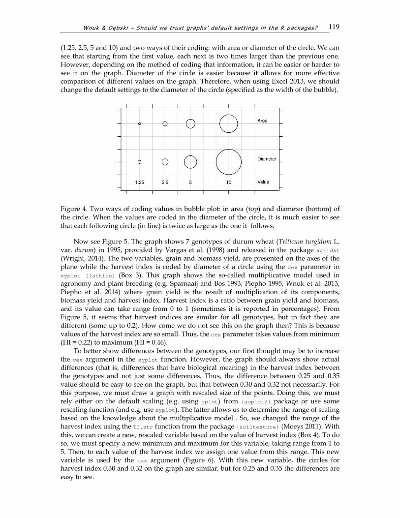
For bubble plot, it is crucial whether we use diameter or area of the circle. Many programs, including R, use diameter of the circle (sometimes reported as radius). However, in the latest version of spreadsheet Microsoft® Excel 2013, we can create this graph with area of the circle as the default. According to many researchers, coding value of the third variable in the area of the symbols is not effective (e.g. Cleveland and McGill 1984a, 1985, Cleveland 1993, pp. 142-145, Cleveland 1994, pp. 268-269, Rougier et al., 2014). It is not as accurate as in the case of their diameter, as can be seen in Figure 4. The graph presents a set of four values
Wnuk & Dębski – Shou ld we t rust graphs ' defau lt set t ings in the R packages?
119
(1.25, 2.5, 5 and 10) and two ways of their coding: with area or diameter of the circle. We can see that starting from the first value, each next is two times larger than the previous one. However, depending on the method of coding that information, it can be easier or harder to see it on the graph. Diameter of the circle is easier because it allows for more effective comparison of different values on the graph. Therefore, when using Excel 2013, we should change the default settings to the diameter of the circle (specified as the width of the bubble).
Figure 4. Two ways of coding values in bubble plot: in area (top) and diameter (bottom) of the circle. When the values are coded in the diameter of the circle, it is much easier to see that each following circle (in line) is twice as large as the one it follows.
Now see Figure 5. The graph shows 7 genotypes of durum wheat (Triticum turgidum L. var. durum) in 1995, provided by Vargas et al. (1998) and released in the package agridat (Wright, 2014). The two variables, grain and biomass yield, are presented on the axes of the plane while the harvest index is coded by diameter of a circle using the cex parameter in xyplot {lattice} (Box 3). This graph shows the so-called multiplicative model used in agronomy and plant breeding (e.g. Sparnaaij and Bos 1993, Piepho 1995, Wnuk et al. 2013, Piepho et al. 2014) where grain yield is the result of multiplication of its components, biomass yield and harvest index. Harvest index is a ratio between grain yield and biomass, and its value can take range from 0 to 1 (sometimes it is reported in percentages). From Figure 5, it seems that harvest indices are similar for all genotypes, but in fact they are different (some up to 0.2). How come we do not see this on the graph then? This is because values of the harvest index are so small. Thus, the cex parameter takes values from minimum (HI = 0.22) to maximum (HI = 0.46).
To better show differences between the genotypes, our first thought may be to increase the cex argument in the xyplot function. However, the graph should always show actual differences (that is, differences that have biological meaning) in the harvest index between the genotypes and not just some differences. Thus, the difference between 0.25 and 0.35 value should be easy to see on the graph, but that between 0.30 and 0.32 not necessarily. For this purpose, we must draw a graph with rescaled size of the points. Doing this, we must rely either on the default scaling (e.g. using gplot) from {ggplot2} package or use some rescaling function (and e.g. use xyplot). The latter allows us to determine the range of scaling based on the knowledge about the multiplicative model . So, we changed the range of the harvest index using the TT.str function from the package {soiltexture} (Moeys 2011). With this, we can create a new, rescaled variable based on the value of harvest index (Box 4). To do so, we must specify a new minimum and maximum for this variable, taking range from 1 to 5. Then, to each value of the harvest index we assign one value from this range. This new variable is used by the cex argument (Figure 6). With this new variable, the circles for harvest index 0.30 and 0.32 on the graph are similar, but for 0.25 and 0.35 the differences are easy to see.
Communicat ions in Biometry and Crop Sc ience , 11 (2)
120
Figure 5. This bubble plot shows seven genotypes of durum wheat (in three replications) in 1995. The x-axis represents above-ground biomass yield (t ha-1) while the y-axis represents grain yield (t ha-1). The values of harvest index (HI) are presented using the cex parameter; it is because the values of the harvest index are small, we do not see any differences between the genotypes.The legend on the right presents genotypes of durum wheat, and the legend on the left presents the size of the circle (harvest index).
Figure 6. This bubble plot shows the same data as those in Figure 5, but this time values of harvest index were rescaled using TT.str function from he {soiltexture} package (Moeys 2011). It was done to better present actual differences in the harvest index than with the cex parameter.
Wnuk & Dębski – Shou ld we t rust graphs ' defau lt set t ings in the R packages?
121
Box 3: Bubble plot created in {lattice} package with cex parameter used to represent values of harvest index
print(p1a, panel.width = list(x = 1.5, units = "in"), split = c(1, 1, 2, 1), more =
TRUE)
print(p1b, panel.width = list(x = 3.9, units = "in"),split = c(2, 1, 2, 1), more =
FALSE)
Communicat ions in Biometry and Crop Sc ience , 11 (2)
122
Box 4: Bubble plot created in {lattice} package with cex parameter used to represent rescaled values of harvest index by TT.str function from {soiltexture} package
print(p2a, panel.width = list(x = 1.5, units = "in"),
split = c(1, 1, 2, 1), more = TRUE)
print(p2b, panel.width = list(x = 4, units = "in"),
split = c(2, 1, 2, 1), more = FALSE)
Wnuk & Dębski – Shou ld we t rust graphs ' defau lt set t ings in the R packages?
123
We can also produce a bubble plot using gplot from {ggplot2} package. This function does not have the same drawbacks as xyplot because it automatically scales the size of the symbols and adds the legend, which is an advantage of this function and an example of good default settings (Figure 7; see also Box 5). However, as we mentioned before (see example 1), symbols on the plot should provide high visual distinguishability. The filled symbols can fail to do this because they are more likely to overlap than the unfilled symbols (e.g. Cleveland 1994, pp. 50-52, 160-164, 234-239, Kozak 2010, Krzywinski and Wong 2013). This is especially inappropriate for bubble plot because smaller circles can be hidden by large ones (Figure 8). Fortunately, this is not the case in Figure 7, but mainly because of a smaller number of the points on the graph. In bubble plot (but also in other graphs), the edges of the points should be visible in order to avoid hiding the observation and reducing their overlap (e.g. Harris 1999, pp. 61, Jacoby 1998, pp. 33-37). However, when we use filled symbols (not only for bubble plot) we must ensure that such problems with overlapping the observation do not occur.
Figure 7. This bubble plot shows the same data as those in Figures 5 and 6, but was constructed in the {ggplot2} package. The values of the harvest index were automatically rescaled in the qplot function. In default settings, symbols are filled, so they are more likely to overlap than unfilled symbols.
Box 5: Bubble plot created in {ggplot2} package with size parameter to represent values of harvest index, a default scaling in {ggplot}
Communicat ions in Biometry and Crop Sc ience , 11 (2)
124
Figure 8. Two ways of presenting data: unfilled symbols (bottom row) and filled symbols (upper row). Note that some of the observations are hidden when filled symbols are used.
CONCLUSION
Scientific literature is full of flawed graphs. Reasons for this are numerous, and one of them is inappropriate default settings in graphical software. Our study is not general since we analyzed only several functions in Excel and R, but there are many other programs that suffer from the very same weakness. Many other default settings can be considered as questionable choices. For example, Statistica and MATLAB use trick marks directed to the inside of the plotting region while they should be directed outside of the plot in order not to conflict with data points (e.g. Cleveland 1994, pp. 31-34, Jacoby and Schneider 2010). In an earlier version of Microsoft Excel (Excel 2003, which is still in use), graphs were created with dark grey background as default; also ggplot2 package (Wickham 2009) offers light grey background. However, in many other programs like Statistica, Excel versions starting from 2007, and {graphics} or {lattice} packages in R, a background of a graph is white or transparent. It allows the user to focus on the data without any distractions. It seems to be the best choice (e.g. Few 2004, pp. 187-188, 210-201, Jacoby and Schneider 2010, Kozak 2010). However, according to some researchers the background of the graph with any color (but with a bright shade) can be useful in some, very specific situations. A subtle fill of color can be helpful when one uses bright colors of symbols or bars (e.g. Few 2004, pp. 210-211). According to Wickham (2008), light gray background creates a feeling that the graph is a consistent visual unit. He believes that a graph with gray background is better because it shares color (in a typographical sense) with text. Therefore, we do not have a situation where a graph with a bright white background suddenly jumping out from text. This is an open issue, and probably it is a matter of subjectivity. Undoubtedly, however, backgrounds in strong colors, gradients, shadings or with pictures are seldom a good idea.
Default settings usually tempt us to assume that we do not need to worry about the graph because the software will do the whole job for us. Not everyone knows (or wants to know) the detailed rules of proper construction of scientific graphs. Probably many users consider it a waste of time; however, incorrect or poor graphs can mislead users and lead to false conclusions. Darrell Huff (1954) in his famous book ”How to lie with statistics” emphasized this. We should always remember about accuracy of all elements of the graph. Graphs in science play an important role of conveying important information. We should not, then, uncritically base on default settings of graphical packages because we showed in the paper that this can end with graphs that can fail to convey this message.
Wnuk & Dębski – Shou ld we t rust graphs ' defau lt set t ings in the R packages?
125
REFERENCES
Basford K.E. (1982). The use of multidimensional scaling in analysing multi-attribute genotype response across environments. Australian Journal of Agricultural Research 33, 473–480.
Bergman L.D. Rogowitz B.E., Treinish L.A. (1995). A rule-based tool for assisting colormap
Cleveland W.S. (1993). Visualizing Data. Hobart Press, Summit, NJ, USA.
Cleveland W.S. (1994). The Elements of Graphing Data. 2ed. Hobart Press, Summit, NJ, USA.
Cleveland W.S., McGill R. (1984a). Graphical perception: Theory, experimentation, and application to the development of graphical methods. Journal of the American Statistical
Association 79, 531−554.
Cleveland W.S., McGill R. (1984b). The many faces of a scatterplot. Journal of the American
Statistical Association 79, 807−822.
Cleveland W.S., McGill R. (1985). Graphical perception and graphical methods for analyzing scientific data. Science, New Series 229, 828–833.
Comas C., Avilla J., Sarasúa M.J., Albajes R., Ribes-Dasi C. (2012). Lack of anisotropic effects in the spatial distribution of Cydia pomonella pheromone trap catches in Catalonia, NE
Spain. Crop Protection 34, 88−95.
Harris R.L. (1999). Information graphics: A comprehensive illustrated reference. Management Graphics, Atlanta, Georgia, U.S.A., Second printing.
Huff D. (1954). How to lie with statistics. WW Norton, New York, MY, USA.
Few S. (2004). Show me the numbers: Designing tables and graphs to enlighten. Oakland, CA: Analytics Press.
Jacoby W.G. (1998). Statistical graphics for visualizing multivariate data. Sage University Papers
Series. No. 07−120.
Jacoby, W.G., Schneider, S.K. (2010). Graphical displays for political science journal articles. Prepared for presentation at the Visions in Methodology Conference. University of
Iowa, March 18−20, 2010.
Kozak M. (2010). Basic principles of graphing data. Scientia Agricola 67, 483−494.
Kroonenberg P.M., Basford K.E.B. (1989). An investigation of multi-attribute genotype response across environments using three-mode principal component analysis. Euphytica 44, 109–123.
Krzywinski M., Wong B. (2013). Points of view: Plotting symbols. Nature methods 10, 451−451.
Lamkey C.M., Lorenz A.J. (2014). Relative effect of drift and selection in diverging
populations within a reciprocal recurrent selection program. Crop Science 54(2), 576−585.
Melchinger A.E., Schipprack W., Mi X., Mirdita V. (2015). Oil content is superior to oil mass for identification of haploid seeds in maize produced with high-oil inducers. Crop
Science 55, 188−195.
Moeys J. and contributions from Shangguan W. (2011). soiltexture: Functions for soil texture plot, classification and transformation. R package version 1.2.2. http://CRAN.R-project.org/package=soiltexture
Morrison M.J., Cober E.R., Frégeau-Reid J.A., Seguin P. (2015). Changes in lutein and tocopherol concentrations in soybean cultivars released across seven decades in the
short-season region. Crop Science 55, 312−319.
Piepho H.P. (1995). A simple procedure for yield component analysis. Euphytica 84, 43−48.
Piepho H.P., Müller B.U., Jansen C. (2014). Analysis of a complex trait with missing data on the component traits. Communications in Biometry and Crop Science 9, 26–40.
Communicat ions in Biometry and Crop Sc ience , 11 (2)
126
R Core Team (2015). R: A language and environment for statistical computing. R Foundation for Statistical Computing, Vienna, Austria. URL http://www.R-project.org/.
Rougier N.P., Droettboom M., Bourne P.E. (2014). Ten simple rules for better figures. PLoS Computational Biology 10, e1003833.
Sarkar D. (2008). lattice: Lattice Graphics. R package version 0.18-3. http://CRAN.R-project.org/package=lattice
Sparnaaij L.D., Bos I. (1993). Component analysis of complex characters in plant breeding I. Proposed method for quantifying the relative contribution of individual components to
variation of the complex character. Euphytica 70, 225−235.
Su Y.-S. (2008). It’s easy to produce chartjunk using Microsoft® Excel 2007 but hard to make good graphs. Computational Statistics and Data Analysis 52, 4594–4601.
Timsina J., Humphreys E. (2006). Performance of CERES-Rice and CERES-Wheat models in rice–wheat systems: A review. Agricultural Systems 90, 5–31.
Vargas M., Crossa J., Sayre K., Renolds M., Ramirez M.E., Talbot M. (1998). Interpreting genotype x environment interaction in wheat by partial least squares regression. Crop Science 38, 679–689.
Wickham H.A. (2008). Practical tools for exploring data and models. ProQuest.
Wickham H.A. (2009). ggplot2: elegant graphics for data analysis. Springer New York.
Wnuk A., Górny A.G., Bocianowski J., Kozak M. (2013). Visualizing harvest index in crops. Communications in Biometry and Crop Science 8, 48–59.
Wright K. (2014). agridat: Agricultural datasets. R package version 1.9 http://CRAN.R-project.org/package=agridat
Validi S., Bhattacharya, A., Byrne, P.J. (2015). A solution method for a two-layer sustainable
supply chain distribution model. Computers & Operations Research 54, 204−217.
Yandell B.S. (2007). Graphical data presentation, with emphasis on genetic data. Hortscience
42, 1047−1051.
Zaman T.R., Herbrich R., van Gael J., Stern D. (2010). Predicting information spreading in Twitter. In Workshop on Computational Social Science and the Wisdom of Crowds, NIPS.