MULTICORE/MULTI-GPU ACCELERATED SIMULATIONS OFMULTIPHASE COMPRESSIBLE FLOWS USING WAVELET
ADAPTED GRIDS∗
DIEGO ROSSINELLI† , BABAK HEJAZIALHOSSEINI† , DANIELE G. SPAMPINATO† , AND
PETROS KOUMOUTSAKOS†
Abstract. We present a computational method of coupling average interpolating wavelets withhigh-order finite volume schemes and its implementation on heterogeneous computer architecturesfor the simulation of multiphase compressible flows. The method is implemented to take advantageof the parallel computing capabilities of emerging heterogeneous multicore/multi-GPU architectures.A highly efficient parallel implementation is achieved by introducing the concept of wavelet blocks,exploiting the task-based parallelism for CPU cores, and by managing asynchronously an array ofGPUs by means of OpenCL. We investigate the comparative accuracy of the GPU and CPU basedsimulations and analyze their discrepancy for two-dimensional simulations of shock-bubble interac-tion and Richtmeyer–Meshkov instability. The results indicate that the accuracy of the GPU/CPUheterogeneous solver is competitive with the one that uses exclusively the CPU cores. We report theperformance improvements by employing up to 12 cores and 6 GPUs compared to the single-coreexecution. For the simulation of the shock-bubble interaction at Mach 3 with two million grid points,we observe a 100-fold speedup for the heterogeneous part and an overall speedup of 34.
1. Introduction. Heterogeneous, CPU/GPU based computer architectures pro-vide us today with unprecedented computational power for the simulation of complexphysical systems. We need, however, to develop suitable methods and algorithms toharness these capabilities. We can only stress the importance of an integrative de-velopment of computational methods and software that takes into consideration thehardware architecture. In turn, synchronizing the developments of methods, softwareand hardware holds the promise for even larger advances in all components involved.
A traditional testbed for the development of computational methods is fluid me-chanics. The equations of fluid mechanics involve several classes of PDEs, and overthe years a number of benchmark problems have been established for the validation ofnovel numerical methods. In fluid mechanics, exploiting the capabilities of computerarchitectures with thousands of cores has enabled simulations involving billions [27] ofvariables, resolving scales at Re numbers that have not been possible before. In recentyears the advent of graphics processing units (GPUs) has provided another option foraccelerated massively parallel flow simulations; albeit sometimes the best performanceis obtained at the price of a reduced accuracy. A number of different CFD methodshave been successfully implemented on GPUs such as marker and cell [46], finitedifference/volume schemes [17, 29], Lattice–Boltzmann [6], and vortex methods [42].These simulations rely on translating computational methods into intensive and local-ized computations that take advantage of the single-instruction-multiple-data (SIMD)
∗Submitted to the journal’s Software and High-Performance Computing section May 20, 2010;accepted for publication (in revised form) November 22, 2010; published electronically March 1, 2011.
http://www.siam.org/journals/sisc/33-2/79593.html†Department of Computational Science, ETHZ, CH-8092, Zurich, Switzerland ([email protected].
MULTICORE/GPU SIMULATIONS ON WAVELET ADAPTED GRIDS 513
capabilities of the GPUs, resulting in some cases in up to two orders of magnitudespeedups over the corresponding CPU-only implementations [42].
The sheer number of processors and the corresponding number of computationalelements often mask a key issue regarding the economy of flow simulations usinguniform grids. Flow simulations that exhibit high parallel efficiency benefit fromthe regularity of structured grids that can readily translate into effective computerimplementations by means of data parallelism. This efficiency, however, does nottranslate into short time to solution as the grid regularity is not commensurate withthe multitude of scales often associated with fluid mechanics problems. Hence, seem-ingly paradoxically, high efficiency parallel flow simulations, using uniform grids, willnot be sufficient to address in the foreseeable future problems of engineering interestsuch as the flow around an aircraft. We believe that this situation can be remediedby developing computational methods that employ temporal and spatial adaptivitywhile at the same time allow for implementations that can take advantage of moderncomputer architectures.
A number of computational methods have been developed in the last twenty yearsthat dynamically adjust the resolution of computational elements to match the physi-cal scales. Methods such as adaptive mesh refinement (AMR) [5, 35] or wavelet basedmultiresolution techniques [22, 30, 39, 47] have been developed to this end. AMRtechniques support unstructured grids and can accommodate different grid orienta-tions, while wavelet methods provide higher compression ratios and allow for efficientcomputations by the use of fast wavelet transforms. Wavelets are becoming a tool ofchoice for CFD (see [47] and references therein), and they have been extended to themultiresolution representation of geometries using level sets [4]. Wavelets, while effi-cient in providing spatial adaptivity, present a number of challenges for their efficientparallelization, making them subject to several efforts in the last ten years that in turnhave resulted in hardware-accelerated wavelet transforms. The first GPU based two-dimensional fast wavelet transform (FWT) was introduced in 2000 [25]. Since then,many different parallel implementations have been proposed both on multicore archi-tectures such as the Cell BE [2] and on GPUs [48]. These efforts, however, have beenrestricted to the full FWT. The full FWTs are used mainly in signal processing to findall the detail coefficients of a data set, and the subsequent processing is performed inthe wavelet space, directly modifying the detail coefficients. However, wavelet-basedadaptive PDE solvers differ in their computational implementation with respect towavelet-based signal processing techniques. First, when wavelets are used for solvingan initial value problem, one does not know in advance how the solution will evolve;therefore, the full time-space FWTs cannot be employed. Second, operations involv-ing nonlinear terms (e.g., the convection term in the Navier–Stokes equations) needto be efficiently performed. This is not always possible when working in the waveletspace, and it is meaningful to keep the representation of the solution in the physi-cal space and use the detail coefficients only to readapt the grid. In this approachnot every detail coefficient is needed but only the ones directly related to points ofthe adapted grid (i.e., the finest scaling coefficients of the adapted grid). When thesolution is represented in the physical space, a third difference between signal pro-cessing and PDE solvers becomes evident. In the latter, the choice of the wavelets isoften limited to the biorthogonal ones associated with symmetric and smooth scalingfunctions. Conventional choices are average interpolating wavelets, first or secondgeneration interpolating wavelets, or B-spline wavelets. Furthermore, the grid has toundergo refinement and compression very frequently as extra care is needed to capture
all the emerging scales.The parallel implementation of wavelet-based adaptive PDE solvers is hindered
by their, inherently sequential, nested structure. This difficulty limits their effectiveimplementation on multicore architectures, and the limitation is even more severe forheterogeneous multicore/multi-GPU architectures. In the context of plain multi-corearchitectures, it has been recently demonstrated that this issue can be relaxed byintroducing the concept of wavelet blocks and by employing task-based parallelism[43]. To the present knowledge of the authors, there are no works so far that addressthe issues of solving PDEs on a wavelet-based adapted grid with heterogeneous multi-GPU/multicore machines.
In this work we introduce such a solver for the simulation of multiphase compress-ible flows and report accuracy issues and performance gains for benchmark problemsof shock-bubble interaction and Richtmeyer–Meshkov instability. We remark that thelocality of flow structures, inherent to compressible flow simulations, is ideally suitedto the locality of data structures that can be exploited by GPUs, as has been shownin the work of Elsen, LeGresley, and Darve [17], Brandvik and Pullan [8], and Hagen,Lie, and Natvig [21]. These works mainly focused on single phase flows on uniformresolution or unstructured grids, while the reduced accuracy of the GPUs has not beenextensively addressed. The present work addresses the simulations of compressible,multiphase flows on multicore and multi-GPU architectures using grids adapted viawavelet analysis of the flow structures.
The paper is structured as follows: in section 2 we present the governing equationsof multiphase compressible flows and their finite volume discretization. We brieflyintroduce wavelet-based multiresolution analysis to construct an adaptive grid andsolve the flow equations in section 3. We then introduce a data structure referred toas a wavelet block to reduce the granularity of the method and make it more suitablefor parallel execution. In section 4 we propose a way to couple CPU cores withan array of GPUs to obtain a heterogeneous solver. We report the strong scalingand a detailed study on the accuracy/discrepancy for the Sod shock-tube benchmarkand shock-bubble interaction at different Mach numbers as well as the Richtmeyer–Meshkov instability in section 5.
2. Governing equations and uniform resolution discretization. Wemodelan inviscid compressible flow as described by the Euler equations using the one-fluidformulation [38]:
(2.1)
∂ρ
∂t+∇ · (ρu) = 0,
∂(ρu)
∂t+∇ · (ρu⊗ u+ pI) = 0,
∂(ρE)
∂t+∇ · ((ρE + p)u) = 0,
with ρ being the density, u the velocity vector, p the pressure, and E the total energyof the fluid per unit mass. Closure of this system of equations is enforced by ensuringthat the two phases, gas and liquid fluid, follow the ideal gas equation of state,
(2.2) p = (γ − 1)ρ
(E − 1
2|u|2
),
with γ being the ratio of specific heats of each phase.
MULTICORE/GPU SIMULATIONS ON WAVELET ADAPTED GRIDS 515
Here, the interface is represented by a color function φ, where φ < 0 representsphase 2 and φ ≥ 0 represents phase 1.
The evolution of the interface is governed by a linear advection equation of theform
(2.3)∂φ
∂t+ u ·∇φ = 0.
The specific heat ratio γ couples the evolution of the interface to the system of equa-tions (2.1)–(2.2), and it is based on φ:
γ(φ) = γphase1Hε(φ) + γphase2(1−Hε(φ)),(2.4)
Hε(φ) =
0, φ < −ε,12 + φ
2ε +12π sin(πφε ), |φ| ≤ ε,
1, φ > ε,(2.5)
where the mollification length ε is constant. The governing equations (2.1) can becast in the form
(2.6) qt +∇ · f(q) = 0,
where the subscript t denotes the time derivative. This system of equations requiresan initial condition of the form q(x, 0) = q0(x) and appropriate boundary conditions.The evolution of the fluid under this system of equations often leads to the develop-ment of shocks and contact discontinuities in the solution vector q, and therefore theintegral form of (2.6), i.e.,
(2.7)
∮(qdx − f(q)dt) = 0,
is better suited for numerical simulations. If the computational domain is uniformlydiscretized by finite volumes, then cell averages {qn
i } at time t = tn and the flux
(2.8) Fi±1/2 =1
∆t
∫ tn+1
tnf(qn
i±1/2(t))dt
determine the new solution qn+1 at time tn+1 = tn + ∆t. In order to avoid theexpensive Riemann solver [49], Fi±1/2 is approximated by a numerical flux Fi±1/2.
The new cell averages {qn+1i } are found after one simulation step by evaluating the
numerical fluxes and performing a time integration for all the averages:
(2.9) qn+1i = qn
i − ∆t
∆x(Fi+1/2 − Fi−1/2).
Since Fi+1/2 and Fi−1/2 depend on the local cell neighbors of qni , the simulation step
formulated in (2.9) can be seen as a nonlinear uniform filtering at the location of qni .
In this work we use the HLLE [16] numerical flux that has been shown to be wellcapable of capturing isolated shocks and rarefaction waves and is not as computa-tionally expensive as the Riemann solver. We employ a fifth order WENO scheme[33, 28] to reconstruct the primitive quantities and a time-stepper based on the secondorder TVD Runge–Kutta scheme [51]. The interface evolution equation (2.3) is madesuitable for our generic conservative flux-based solver using the method introduced in[45].
3. Wavelet-based adaptive grids. In this work, the creation of adapted gridsis based on average interpolating wavelets. These wavelets belong to the family ofbiorthogonal wavelets and are used to construct a multiresolution analysis (MRA) ofthe quantities of interest. We can use the scale information of the MRA to obtain acompressed representation by performing a thresholding that retains only the scalingcoefficients which carry significant information.
In order to solve the flow equations on adapted grids, we apply standard finitevolume (alternatively finite difference) schemes on the active coefficients. One way tosimplify these operations is to first create a local, uniform resolution neighborhoodaround a grid point and then apply the corresponding finite volume scheme to it.This process in turn requires the introduction of auxiliary grid points, the so-calledghosts. For accuracy and efficiency reasons, the grid has to be readapted as the flowfield evolves. This is done by coarsening some regions and refining some others afterconstructing a new MRA of the flow.
We refer the reader to the appendix for a detailed discussion on how averageinterpolating wavelets are used to solve the flow equations on adaptive computationalgrids.
3.1. Wavelet blocks. The wavelet-adapted grids for solving flow equations areoften implemented with quad-tree or oct-tree structures whose leaves are single scalingcoefficients (i.e., cell averages). The main advantage of such fine-grained trees isthe very high compression rate which can be achieved when thresholding individualdetail coefficients. The drawback of this approach is the large amount of sequentialoperations it involves and the number of memory indirections (or read instructions)necessary to access a group of elements. Even if we keep the grid structure unchangedwhile computing, these grids already perform a great number of neighborhood look-ups. In addition, operations like refining or coarsening single grid points are relativelycomplex and strictly sequential.
In this work, in order to expose more parallelism and to decrease the amount ofsequential operations per grid point, the key idea is to simplify the data structure. Weaddress this issue by coarsening the granularity of the solver, i.e., the atomic elementof the grid, at the expense of a reduction in the compression rate. We introduce theconcept of block of grid points, whose size is one or two orders of magnitude largerin every direction with respect to a scaling coefficient; i.e., in three dimensions, thegranularity of the block is coarser by 3 to 5 orders of magnitude with respect to asingle scaling coefficient. All the scaling coefficients contained in one block have thesame level, and every block contains the same number of scaling coefficients. Thegrid is then represented with a tree which contains blocks, instead of single gridpoints, as leaves (Figure 3.1). The blocks are nested so that every block can besplit and doubled in each direction and blocks can be collapsed into one. Blocksare interconnected through the ghosts and, in the physical space, the blocks havevarying sizes and therefore different resolutions. The block structure of the gridprovides a series of benefits. First, tree operations are now accelerated as they canbe performed in log2(N
1/D/sblock) operations instead of log2(N1/D), where N is the
total number of active coefficients, D is the considered dimensionality, and sblock isthe block size. The second benefit is that the random access at elements inside a blockcan be efficient because the block represents the atomic element. Another advantageis the reduction of the sequential operations involved in processing a local group ofscaling coefficients. The cost c (in terms of memory accesses) of filtering a grid pointwith a filter of size wstencilD in a uniform resolution grid is proportional to wstencilD.
MULTICORE/GPU SIMULATIONS ON WAVELET ADAPTED GRIDS 517
Fig. 3.1. The adapted cell-centered grid is represented with 13 blocks at 3 different resolutions.Every block contains the same number of scaling coefficients (left). The blocks are the leaves of thegrid tree (right).
For a grid represented by a fine-grained tree, the number of accesses is proportionalto c = wstencilD log2(N
1/D), due to the sequential access to the tree nodes. Using thewavelet blocks approach and assuming that sblock is roughly one order of magnitudelarger than wstencil, the ratio of ghosts needed per grid point in order to perform thefiltering for a block is
(3.1) r =(sblock + wstencil)D − sDblock
sDblock≈ D
wstencil
sblock.
Therefore, the number of accesses for filtering one grid point is
c = (1 − r)wstencilD + rwstencilD(log2(N
1/D/sblock))
= wstencilD + wstencilDr(log2(N
1/D/sblock)− 1).(3.2)
As an example we consider a two-dimensional worst case scenario: an adapted gridof four million points that is fully refined everywhere. For N = 222, D = 2 we wantto perform a fifth-order WENO reconstruction; therefore, wstencil = 6. For a uniformresolution grid representation we have c = 12, and for a fine-grained adapted tree wehave c = 132. For a blocked adaptive grid with sblock = 32 we have c ≈ 36. Thismeans that in terms of memory accesses, by using blocks we are 3 times slower thana uniform grid and 3.7 times faster than a fine-grained adapted grid. On average, inplaces where we have an “actual” adaptation of the grid, the speed difference betweenthe block-based and the fine-grained grids becomes substantially larger because of thenumber of ghosts that they need to reconstruct.
We note that none of the blocks overlap with any other block in the physicalspace as the blocks are the leaves of the tree. In order to improve the efficiency offinding the neighbors of a block, we define as neighbors all the blocks adjacent to theone considered. Because of this constraint, the highest jump in resolution allowed(between two adjacent blocks), Lj, is bounded by log2 (sblock/wstencil).
3.2. Local time stepping (LTS) for wavelet adapted grids. Additionalspeedup is obtained by combining spatially adapted grids with local time-stepping(LTS) schemes, which advance in time the properties of the computational elementsby taking into consideration their corresponding different time scales necessary for astable discretization. LTS schemes have been shown to speed up the computation byone order of magnitude or more depending on the number of blocks at each level ofresolution [13, 14, 1, 44].
Recently, we proposed a new perspective on LTS schemes [23] that allows us toreformulate existing LTS algorithms in a simpler way. In this view each computa-tional element of the grid is considered as an independent entity. We associate atime-reconstruction function to every computational element (i.e., cell averages). Thecomputation of the right-hand side is not performed by considering directly the com-putational elements, but by considering their time-reconstructed values. Each blockin the grid is also associated with a state diagram, which is repeatedly traversed whenthe grid elements undergo a time integration. The operations involved in the statetransitions of a grid point are deduced by imposing some interpolating postcondi-tions on the reconstruction functions. In the new formulation we relax, or almosteliminate, the coupling between the evaluation of right-hand sides, the update of theblocks, and the recursive iteration through the blocks. This enables us to identifythe compute-intensive parts of the LTS schemes and therefore obtain, in combina-tion with the block-based representation of the grid, an effective implementation formulticore/multi-GPU machines.
Even though LTS schemes are capable of dramatically decreasing computing time,they present a major shortcoming: the grid blocks have to be grouped by their timescales, and therefore multiple groups cannot be processed in parallel. This meansthat there are additional synchronization points in the algorithm, and the degree ofparallelism for processing a group of blocks is limited by the group size.
4. Implementation on multi-GPU/multicore architectures. In this sec-tion we discuss the retainment of scales on the grid, introduce OpenCL for GPUs, andexplain the parts of the algorithm that have been redesigned for multi-GPU execution.Finally, we present the OpenCL-based GPU implementation of the solver.
4.1. One simulation step. In order to keep the grid adapted to the evolv-ing solution, a simulation step modifies the grid in three different stages [32]—therefinement stage, the computing stage, and the compression stage—as illustrated inFigure 4.1 (left).
The refinement stage refines the grid in those regions where small scales areexpected to emerge. In practice, we perform a one-level FWT to compute the finestdetail coefficients of the grid. If the maximum detail over all detail coefficients withina block is bigger than εrefine, we trigger the split of the block, and we fill the newblocks by performing a one-level inverse wavelet transform of the scaling coefficientsof the old block.
In the computing stage we perform the time integration of the solution by com-bining finite volume schemes and the LTS scheme. Note that in this stage the gridstructure remains unchanged. It is desired (and empirically observed) that most ofthe execution time is spent here. This stage generally takes between 80% and 98%of the execution time, depending on the problem, the chosen wavelet type, and othercomputational parameters. This means that the refinement/compression stage intro-duces a time overhead between 1–10%, which is the cost for maintaining a dynamicallyadapted grid.
Once the numerical time integration is performed, the grid is further processedin the compression stage. In this stage we perform another one-level FWT to retrievethe new detail coefficients; based on those coefficients we decide where to coarsen thegrid by collapsing blocks. We traverse the grid considering, at once, all the blockssharing the same parent. If the maximum detail over all the children blocks that sharethe same parent is less than εcompress and if the local resolution jump is less than the
MULTICORE/GPU SIMULATIONS ON WAVELET ADAPTED GRIDS 519
Fig. 4.1. Stages to perform one simulation step (left) and data flow diagram for evaluating theright-hand side in the computing stage (right).
maximum allowed, then we collapse the children. The data of the new leaf is createdby performing a one-level FWT of the scaling coefficients within the blocks.
4.2. The computing stage. In order to integrate the solution in time, thecomputing stage performs one global step of the LTS scheme. We can identify threedifferent operations during the grid traversing of the LTS: time-reconstruction of thequantities, evaluation of the right-hand side, and update of the quantities by time inte-gration. Time-reconstruction and integration are not computationally very expensiveas they involve a small number of multiplications and additions per grid point. Be-cause of their poor/medium computing intensity, it is likely that the performance ofthese two operations are bounded by the speed of accessing the grid points in memory.The evaluation of the right-hand side is performed after the time-reconstruction andis computationally expensive. This consists in reconstructing the ghosts, convertingthe conserved quantities into primitive quantities, WENO reconstructing five quanti-ties (ρ, u, v, E,φ) in two directions, evaluating HLLE fluxes for all the quantities, andsumming them, as illustrated in Figure 4.1 (right).
WENO reconstructions involve a considerable amount of computation. A WENOreconstruction of order 2r − 1 can be written as [28]
(4.1) f+j+1/2 =
r−1∑
k=0
ωkqrk(fj+k−r+1, . . . , fj+k),
where {fj} are primitive quantities and
qrk(g0, g1, . . . , gr−1) =r−1∑
l=0
ark,lgl,(4.2)
ωk =αk∑r−1i=0 αi
,(4.3)
αk =Cr
k
(ε + ISk)p, k = 0, 1, . . . , r − 1,(4.4)
with ε = 10−6 and p = 2 in our computations. For a fifth order WENO reconstruction,r = 3 and ark,l, C
rk are obtained from Table 4.1, and the indicators of smoothness ISk
Table 4.1Coefficients of the 5th order WENO reconstruction.
ar=3k,l Cr=3
k
k l = 0 l = 1 l = 2 -0 1/3 -7/6 11/6 1/101 -1/6 5/6 1/3 6/102 1/3 5/6 -1/6 3/10
for r = 3 and k = 0, 1, 2 are computed as
IS0 =13
12(fj−2 − 2fj−1 + fj)
2 +1
4(fj−2 − 4fj−1 + 3fj)
2,(4.5)
IS1 =13
12(fj−1 − 2fj + fj+1)
2 +1
4(fj−1 − fj+1)
2,(4.6)
IS2 =13
12(fj − 2fj+1 + fj+2)
2 +1
4(fj − 4fj+1 + 3fj+2)
2.(4.7)
Because the reconstructed values are shared by adjacent cells in a block, we have toperform 10 WENO reconstructions per cell per block (the “south” and “west” cellfaces for five scalar quantities).
The evaluation of the numerical flux HLLE is compute-intensive. It reads
(4.8) Fj+1/2 =
f−j+1/2, a−j+1/2 > 0,
f+j+1/2, a+j+1/2 < 0,
a+j+1/2f
−j+1/2−a−
j+1/2f+j+1/2+a+
j+1/2a−j+1/2(u
+j+1/2−u−
j+1/2)
a+j+1/2−a−
j+1/2
otherwise,
where a− and a+ are the left-running and right-running characteristic velocities, re-spectively.
4.3. OpenCL. OpenCL stands for “open computing language” and is a specifi-cation for programming on heterogeneous (parallel) computing devices. An extensiveintroduction to the OpenCL specification can be found in [36]. Here we restrict our-selves to discussing OpenCL for GPU computing. In this case OpenCL is similar tothe CUDA framework [37], and, moreover, it provides portability between differentGPU hardware. The OpenCL specification consists mainly in the description of threemodels: the execution model, the memory model, and the programming model. Theexecution model is split into two parts: kernels that execute on one or more OpenCLdevices (in our case the GPUs) and a host program that executes on the host (CPU).The host program defines the context for the kernels and manages their execution.When a kernel is submitted for execution by the host, the OpenCL devices are capa-ble of running multiple instances of the same kernel in parallel. One kernel instanceis called a work item. Work items are executed in parallel and can process differentdata. One can submit kernels for execution, memory commands, and synchroniza-tion commands to an OpenCL device with a command queue. When the host placescommands into the command queue, the queue schedules them onto the device. Avery appealing feature of command queues is that they can support out-of-order ex-ecution: commands that are issued in order do not wait to complete before the nextcommands execute. Submissions of commands to a queue return event handles, theOpenCL events. They are used to describe the dependency between commands, tomonitor the execution, and to coordinate execution between the host and the devices.
MULTICORE/GPU SIMULATIONS ON WAVELET ADAPTED GRIDS 521
4.4. OpenCL for GPUs. Optimal GPU performance dictates that the paral-lelism must be expressed with fine-grained homogeneous work items. These devicesaremany-core architectures, and each core processes work items in a single-instructionmultiple-data (SIMD) fashion. As the number of resources available per core is verylimited, the work items have to be fine-grained, with many threads performing smallprocessing on a small amount of data. Because of their fine-grained properties, thelifetime of a work item is expected to be in the order of microseconds or less. At thesame time, the number of work items is expected to be large—at least one order ofmagnitude larger than the amount of cores. Considering this and the fact that cur-rently GPUs are single-instruction multiple-threads (SIMT) machines, it is clear thatoptimal performance is achieved when work items are homogeneous, i.e., when thesmall tasks perform the same operations. The performance gain achieved by GPUs isvery fragile: severe performance degradation can be observed when work items requiretoo many resources (i.e., they are not fine-grained) or contain too many condition de-pendent instructions (inhomogeneous work items) or do not access memory with theright pattern (memory-indirections, traversing sequential data structures, etc.).
4.5. Heterogeneous computing with multicore and multi-GPU. Theabove-mentioned performance fragility of the GPUs prompted us not to aim for acomplete GPU implementation but instead to accelerate the computing stage, whichis the most expensive part of the algorithm, using multiple GPUs. In order to achievethis, a number of modifications were necessary in our original algorithm. The mainreason is that one single block does not expose enough fine-grained work items to keepall the GPU cores busy, as the block size is in the range of 8 × 8 and 32 × 32 gridpoints, while current generation of GPUs have hundreds of cores (on the computinghardware considered in this work we have 240 cores per GPU). Moreover, work itemswithin a block are not homogeneous: grid points close to the block faces need toreconstruct ghosts in order to evaluate the right-hand side. Because of the ghosts’reconstruction, these work items demand a substantial number of extra registers tocarry out the summation of a dynamic-sized array. This request of extra resourcesmakes these work items not fine-grained anymore, which leads to a reduced numberof active (concurrent) work items.
In order to achieve better performance, we pack blocks into input tokens, andwe reconstruct ghosts on the CPU. We then process the tokens on the GPUs. Theadvantage of working with packs of blocks (ranging from 4 × 4 to 20 × 20 blocks) isthat we expose enough work items to keep all the GPU cores busy. The CPU prepa-ration of the tokens is multithreaded and is expressed with task-based parallelism.As illustrated in Figure 4.2, input tokens include not only grid points of blocks butalso ghosts. The calculation of ghosts is nested in parallel tasks spawned inside thecreation of input tokens, which are also parallel tasks. The ghosts’ reconstructiontasks are not load balanced, as the time complexity for reconstructing ghosts dependson the local structure of the grid. However, dynamic load balance is achieved by theWork Stealing algorithm [7], which schedules these tasks in a near-optimal way. Assoon as one input token is ready to be processed, it is asynchronously scheduled byOpenCL for an out-of-order GPU execution. In Figure 4.2 it is shown that the GPUprocessing fills output tokens, which contain the right-hand side of the flow quan-tities. The GPU-CPU transfer of the output tokens is asynchronously scheduled byOpenCL. When the transfer of one output token is complete, the token is unpacked inparallel and the grid blocks associated with that token are time-integrated using thenew right-hand side values. As the memory resources of GPUs are limited, sometimes
Fig. 4.2. Wavelet blocks are prepared and sent to the GPUs for the evaluation of the right-hand side. The GPU output is then postprocessed to update the solution. The preparation of theinput tokens is fully multithreaded and is responsible for reconstructing the ghosts, packing theblocks into tokens and sending them to the GPUs. Once the GPUs have processed some tokens, thepostprocessing stage unpacks the output token in a multithreaded fashion.
it is not possible to create and submit all the necessary input tokens at once. In thatcase the program waits for a GPU to be done with some of the tokens and reuses theallocated GPU memory to make new input tokens. As tokens are stored on both CPUand GPUs, their memory layout is divided into a CPU part and a GPU part. As wedesire asynchronous CPU-GPU transfer of the tokens, the CPU part of each token isallocated through OpenCL requests for page-locked memory regions. The CPU partof a token consists of several plain two-dimensional arrays, where each entry has fourcomponents (“float4”). During the packing process, these arrays are filled by CPUthreads with the necessary content from the wavelet blocks. This data is then sentto the GPUs and converted into image objects, which represent the GPU part of thetoken. The packing of the tokens consists in the extraction of the relevant quantitiesfrom the grid points, and it is performed by iterating over a group of wavelet blocks.Similarly, to unpack a token we iterate over the associated wavelet blocks and readthe corresponding entries from their arrays.
4.6. Reimplementing the right-hand side evaluation for GPUs. Themost straightforward way of reimplementing the right-hand side evaluation wouldbe to directly map grid-points of one input token to work items and perform allthe computation in one kernel. Since optimal performance on GPUs imposes a highnumber of work items that are fine-grained and homogeneous, we cannot afford a one-to-one mapping. Such a mapping would require many registers, and due to limitedresources this would result in a reduced number of concurrently active work items.Instead, we split the processing into different kernels, as depicted in Figure 4.3: fourkernels for the WENO reconstruction, two kernels for evaluating the HLLE fluxes,and one to sum up the fluxes. This splitting of the GPU processing into multiplekernels introduces an additional overhead associated to their invocation. The largenumber of work items involved in these kernels makes this overhead negligible as ittakes less than 1% of the total execution time (from empirical observations). TheGPU computation starts after the GPU uploads an input token. The four WENOkernels start to process the token in parallel. The group of four WENO kernels can besplit into pairs: one pair performs the reconstruction between the grid points in the
MULTICORE/GPU SIMULATIONS ON WAVELET ADAPTED GRIDS 523
Fig. 4.3. Data flow for the GPU computation. The input data (left) contains the currentsolution. Intermediate data (green blocks) are produced by executing the WENO and HLLE kernels(blue). The final data (RHS) is the result of the SUM kernel.
x-direction, whereas the second pair performs the reconstruction in the y-direction.The first kernel in this pair carries out the “−” side reconstruction whereas the sec-ond one takes care of the “+” side. As soon as the WENO reconstruction in thex-(y-)direction is done, the execution of the kernels computing the HLLE x-(y-)fluxescan take place. Once both x- and y-fluxes are computed, the SUM kernel sums thefluxes in both directions and fills the output token with the right-hand side. At thispoint the output token is ready to be downloaded to the CPU. Except for the lastone, every kernel fills some intermediate data that is subsequently read as input inthe next kernel.
In order to potentially increase data-level parallelism and reduce the number ofinstructions, the computation inside the kernels is expressed with SIMD instructionswith a vector width of four (“float4”). Inside the WENO and HLLE kernels, the workitems are mapped to the work of a cell face. We observed that the WENO kernelstake 48–51 registers per work item, which translates to an occupancy of 0.312 on theconsidered GPU hardware. The HLLE kernel is more expensive in terms of registerusage, as it takes 107 registers per work item, leading to an occupancy of 0.125. Thework items of the SUM kernels are mapped to the work of 2× 2 cells to maximize thereuse of the fluxes. We observed an occupancy of 0.375 using 42 registers per workitem. Both input and intermediate data are represented with image objects, as theWENO and SUM kernels show nontrivial data access patterns.
Control flow instructions could result in different branches among the work items(divergent branches). These branches are absent in the WENO and SUM kernels.Instead, the HLLE kernels show a rate of 0.05 divergent branches per work item. Weexplain this by the presence of three conditional assignments (per kernel) that aretranslated into if-statements.
As illustrated in Figure 4.3 most kernels (even of different types) can be executedin parallel. Our implementation submits these kernels for execution so as to takeadvantage of the newest hardware capability to support parallel execution of differenttypes of kernels [18]. However, it should be noticed that the results reported in thiswork are obtained with GPUs without this capability.
We note that the dependency graph of all the operations involved in processingone token is not trivial (some nodes in the graph have a degree that is higher thantwo). An efficient implementation that follows this dependency graph with the explicituse of synchronization points is challenging, especially if we take into account that
Fig. 5.1. L1 (left) space convergence for uniform and adaptive simulation on multicore andmulti-GPU using different block sizes and a jump in resolution of 2. Number of right-hand sideevaluations versus the absolute L2 norm error using global time stepping (GTS) and local timestepping (LTS) versions of RK2 time stepper (right).
different tokens can be processed at the same time. With OpenCL, however, we donot have to handle these synchronization points explicitly, as we can describe thecomplete sequence of actions by means of the OpenCL events. The submission of thecommands to transfer a token, process it on the GPU, and transfer it back is done inone shot. The events are used by OpenCL to optimally schedule these tasks in orderto achieve a near-optimal execution.
5. Results. In this section we report the accuracy of the heterogeneous solverfor the simulation of the Sod shock-tube benchmark [31] and simulations of shock-bubble interaction and Richtmeyer–Meshkov instability. We highlight the discrepancyin the flow quantities computed on the CPU and the GPU and present the achievedperformance gain with the heterogeneous solver. All the results have been obtainedwith the hardware listed in section 5.4.1 and by using fifth-order average interpolatingwavelets and a maximum resolution jump of two. We have used block sizes of 16×16,24×24, and 32×32 grid points for the shock-tube problem and a block size of 32×32in our two-dimensional simulations.
5.1. One-dimensional benchmark: Sod shock-tube. Figure 5.1 shows theconvergence plots for the Sod shock-tube problem simulated on both multicore CPUand multicore/multi-GPU. We observe that there is no significant difference betweenthe two plots. This test case is a standard benchmark for the accuracy of numericalmethods in solving compressible flows and has an analytical solution. We notice theexpected first-order convergence in space for the L1 (left picture) norm errors usinguniform resolution grids. The discontinuities present in the exact solution of this testcase prohibit convergence orders of more than one in finite volume based methods.This slow convergence can be overcome by using fewer grid points when possible,therefore increasing the convergence rate to 3 in both cases. We note that to achievethe same accuracy (in terms of L1 norm errors), fewer grid points are necessary whenusing smaller block sizes with a jump in resolution of 2. It is clear from Figure 5.1(left picture) that in almost all the cases, the CPU+GPU execution produces the same
MULTICORE/GPU SIMULATIONS ON WAVELET ADAPTED GRIDS 525
accuracy in space as the CPU-only execution. This test case is a standard benchmarkfor the accuracy of numerical methods in solving compressible flows and has an exactsolution [31].
To show the performance improvement obtained with LTS, we present the numberof right-hand side evaluations needed when using global time-stepping (GTS) and LTSversions of RK2 time-stepper versus the L2 norm error in Figure 5.1 (right) in thesimulation of the Sod shock-tube problem up to a given time. It is clear that to achievethe same accuracy (here in the L2 norm), we need fewer right-hand side evaluationswith LTS. In fact, LTS asymptotically improves the complexity of the solver fromO(1/e2) to O(1/e), where e is the upper bound for the L2 error at the final time.Smaller L2 norm errors translate to having finer resolutions (and more adaptivity inspace), and, therefore, the performance improvement obtained by LTS becomes moresignificant at smaller errors.
5.2. Two-dimensional benchmark: Shock-bubble interaction. We per-form simulations of the shock-bubble interaction problem in order to study the dis-crepancy between the solutions of CPU+GPUs and CPU-only executions. Further-more, we report on the achieved speedup using different computer architectures forthe simulations at different Mach numbers.
In the shock-bubble interaction problem a supersonic shock wave in one medium(air) collides with a cylindrical inhomogeneity (helium) with a nonunit ratio of specificheat constants. The generated baroclinic vorticity modifies the interface betweenthe two phases and produces a complex structure of waves in the vicinity of theinhomogeneity.
Fig. 5.2. Density field (top) and the adaptive grid (bottom) in the simulation of the shock-bubbleinteraction at M = 1.2. From left to right: the initial condition, density at the nondimensional timeT = 1, and density at T = 5.
We present the density field as well as the adaptive grid for two simulationsat M = 1.2 and M = 3 in Figures 5.2 and 5.3 at three different times. In these
Fig. 5.3. Density field (top) and the adaptive grid (bottom) in the simulation of shock-bubbleinteraction at M = 3: the initial condition (left), at nondimensional time T = 1.5 (center), and atT = 4 (right).
Fig. 5.4. L1 discrepancy between the solution computed with CPU+GPUs and the CPU oneversus time. Left: M = 1.2. Right: M = 3.
simulations, grid adaptation was driven by the detail coefficients of the density field aswell as the location of the interface. The results ofM = 1.2 andM = 3 simulations arein very good agreement with the experimental and numerical results of [20, 40, 3, 26].
In Figure 5.4 we present the discrepancy in the solution of integration steps us-ing the LTS version of the RK2 time-stepper for M = 1.2 and M = 3 betweenCPU+GPUs and CPU-only executions. We notice that, although the differences inboth cases become smaller in time, those in the M = 1.2 case are higher than thosein the M = 3 case. Since the solution is updated by multiplying the right-hand sideby a small time step, which is on the order of 10−3 nondimensional time units inour two-dimensional simulations, it is more appropriate to consider the relative andabsolute discrepancies of the right-hand side computation stage.
MULTICORE/GPU SIMULATIONS ON WAVELET ADAPTED GRIDS 527
Fig. 5.5. Time evolution of the L1 discrepancy of the right-hand side between CPU+GPUs andCPU executions. Left: M = 1.2. Right: M = 3.
Fig. 5.6. Localization of the GPU-CPU discrepancy in space. Top: M = 1.2. Bottom: M = 3.White/black: low/high L1 relative difference, black = 10−6, chronologically from left to right.
Figure 5.5 shows the L1 relative difference in computing the right-hand side forγ, ρ, ρu, and ρE components of the solution between CPU+GPUs and CPU-onlyexecutions versus time (T ) in the simulation of the shock-bubble interaction at M =1.2 (left) and M = 3 (right). The discrepancy of the right-hand side for the verticalvelocity component v is not shown here, as during the early times of the simulationits value was zero everywhere in the field. We observe that the L1 relative differencein computing the right-hand side remains smaller than 10−5 for both Mach numbers.
We also present the distribution of the relative difference of the flow quantities inspace at three different times in Figure 5.6. We observe that the highest discrepanciesare located in the proximity of the shocks.
We further investigate the discrepancies introduced in the substeps involved incomputing the right-hand side, i.e., the WENO reconstruction, HLLE flux computa-tion, and the summation of fluxes. The space and time averaged relative and absolutedifferences are shown in Figure 5.7 (left), where it is clear that the significant discrep-
Fig. 5.7. Averaged relative and absolute discrepancies in the WENO reconstruction, HLLE fluxcomputation and the summation of fluxes for the simulation of the shock-bubble interaction (left).The histogram of relative and absolute discrepancies produced in WENO reconstruction stage onrandom initial data contains some large discrepancies that are in the order of 10−4 (right).
Fig. 5.8. Histogram of the absolute differences (left) in computing the internal elements of theWENO reconstruction:
∑2i=0 Nωi (orange),
∑2i=0 Nqi (green), result (violet). Histogram of the
absolute differences between single/mixed precision and the reference computations of the internalcomponents in the WENO reconstruction stage (right). The significant errors are eliminated byusing double precision in computing ISi. Little improvement is observed by using double precisionin all the stages of computing ωi.
ancies are generated in the WENO and the HLLE stages. Although the averageWENO discrepancy is similar to that of HLLE, we observe that some of the WENOdiscrepancies can assume values of two orders of magnitude higher than those ofHLLE. Our goal is therefore to analyze the internal elements of the WENO recon-struction stage in detail and to reveal where relatively high discrepancies lie withinthis stage so as to eliminate the significant errors.
We perform the WENO reconstruction with random initial data on the GPU usingOpenCL using single precision as well as on the CPU using double precision as thereference. The histogram of relative and absolute differences is plotted in Figure 5.7(right). We have also performed the same computation on the CPU using OpenCLin single precision and compared it to the reference, and we noticed no significantdifference between the results obtained from the GPU (OpenCL, single precision) andthose from the CPU (OpenCL, single precision). Therefore, in our further analysis ofthe discrepancy we compare our computations on the CPU using OpenCL in singleprecision with those on the CPU using double precision.
In the next step, we investigate the discrepancies introduced by the internal com-putations involved in the WENO reconstruction stage. Figure 5.8 (left) shows the
MULTICORE/GPU SIMULATIONS ON WAVELET ADAPTED GRIDS 529
Fig. 5.9. Evolution of the interfacial perturbation amplitude in time: air/helium at M = 1.52(Meshkov experiment) (left) and helium/air at M = 3 (right).
population distributions of the discrepancies in ωi and qi (i = 0, 1, 2) as well as thehistogram of the discrepancies in the final result of the WENO reconstruction stage,i.e., fj+1/2. It is clear that the distribution of differences of ωi has a larger mean thanthat of qi. By using mixed precision we try to improve some of the stages used to com-pute (4.2)–(4.7). We focus only on the critical cases that generate relatively higherdiscrepancies in plots of Figure 5.8 and use double precision first in all the stages forcomputing ωi, i.e., in (4.2)–(4.4), and then only in the computation of smoothnessindicators, i.e., (4.5)–(4.7). The improvements are presented in the histograms of theFigure 5.8 (right) versus the original single precision computations. It can be ob-served that the significant errors on the rightmost part of this plot are suppressed byusing double precision in computing ωi. We also notice that if we use double precisiononly for the computation of ISi, we maintain almost the same accuracy as we wouldwhen using the double precision for the whole computation of ωi together with savingprocessing time.
5.3. Simulations of the Richtmeyer–Meshkov instability. The Richtmeyer–Meshkov instability (RMI) [41, 9] is another benchmark problem in gas dynamicswhere baroclinic vorticity is generated on the perturbed interfaces by shock-inducedpressure gradients. We validate our solver against the Meshkov experiment [34], whichconsists of a M = 1.52 normal shock wave in air with an Atwood number A = 0.76for the air/helium interface. The initial amplitude of the sinusoidal perturbation isη0 = 0.2 cm with a wavelength λ = 4 cm and a nondimensional amplitude (η = 2πη/λ)of 0.314. Time is nondimensionalized using T = Ma∞t/η0, where a∞ is the speedof sound inside the preshock air. The quantity measured in the literature and in oursimulations is the amplitude η of the interfacial perturbations (defined as half theinterpenetration length) [24]. In Figure 5.9 (left), we present the evolution of η intime using our method and compare with the results found in [24]. The interfaceundergoes the linear stage of RMI with a phase change at later times (T ≈ 18) anddeviates from the linear theory predictions. The results are in good agreement withthose achieved by the front tracking method [19, 11].
In Figure 5.9 (right), we present the evolution of the interfacial amplitude for aM = 3 shock wave in helium interacting with an A = 0.76 interface between heliumand air. We set η0 = 0.125 and λ = 0.5, which gives a nondimensionalized initialamplitude of 1.57 for the interfacial perturbation. The evolution of the interface is
Fig. 5.10. Density field (left) and the adaptive grid (right) of the simulation of Richtmeyer–Meshkov instability at M = 3. Red/blue denote high/low density. Initial condition (top), solutionat T = 7.68 (bottom).
Fig. 5.11. Closeup on the density contours of the Richtmeyer–Meshkov instability simulatedusing CPU with double precision (green) and single precision (orange) as well as CPU+GPUs insingle precision (violet), from left to right. The contours coincide except at later times of thesimulation.
no longer predictable by linear theory and, as the phases are swapped, the amplitudeof the interfacial perturbation does not undergo a phase change as in the air/heliumcase. Until time T ≈ 2 (in our simulation), i.e., when the shock has passed over thewhole interface, the interface is compressed to η ≈ 1.1.
In Figure 5.10 we present the density field and the adapted grid at two differenttimes. It can be observed that the grid adapts to follow the helium/air interfaceand the discontinuities in density, i.e., transmitted and reflected shock waves. Theinitial grid illustrated in Figure 5.10 (top right) contains 70,000 grid points. Afteran execution time of 4 hours, the heterogeneous solver has a grid (bottom right)consisting of 2,000,000 grid points, with 5 levels of resolution.
Figure 5.11 shows a close-up of the contours of density for three different execu-tions of an RMI simulation on the CPU using double and single precision as well as onthe heterogeneous CPU+GPU architecture. We notice that the small discrepanciesappear at very late times in the simulation, these differences mostly exist between thedouble and single precision executions, and they are not as significant between thesingle precision executions on CPU and on CPU+GPUs.
MULTICORE/GPU SIMULATIONS ON WAVELET ADAPTED GRIDS 531
Fig. 5.12. Speedup achieved in computing the right-hand side (left) and in the overall computingstage (right) by multicore/multi-GPU execution (green) and CPU-only execution (orange) on acompute node with 16 cores and 2 GPUs.
5.4. Performance. We compare the performance of the multicore/multi-GPUsolver for the adaptive simulation of a shock-bubble interaction. The results wereobtained using a grid with 7 levels of resolution and about 2,200,000 grid points.We report the strong scaling with respect to multicore and single-core CPU-onlyexecution, and we analyze how strong scaling varies by changing different parameters.Both single-core and multicore CPU-only solvers were profiled using VTune and werefound to be reasonably efficient; they make extensive use of SSE 3 intrinsics to improvethe computing performance as well as the bandwidth and were compiled using IntelC++ Compiler 11.1 with the flags “-O3 -axTW -ip.” The multicore CPU-only solverexploits the task-based parallelism and processes the blocks as in [43]. In this studywe consider two machines: a compute node with 16 cores and 2 GPUs, and a computenode with 12 cores and 6 GPUs.
5.4.1. Performance on 16 CPU cores and 2 GPUs. In Figure 5.12 we showthe speedup for different numbers of wavelet-blocks (and therefore grid points) on amachine with 4 quad-core AMD Opteron 8380 processors (“Shanghai” cores, 2.5 GHz,6 MB L3-cache) and 2 NVIDIA Tesla T10 S1070 (480 GPU cores in total). On theleft we report the speedup for the evaluation of the right-hand side compared to asingle-CPU core only. With 16 cores (orange) and no GPUs we observe a speedup of15, meaning that the solver achieved a strong efficiency of roughly 94%. If we makeuse of two GPUs we get a considerable improvement in the speedup (green) thatmonotonically increases with the number of wavelet blocks. For a simulation thathandles about 2000 blocks (∼ 2, 200, 000 grid points) the GPUs are able to improvethe multicore execution by a factor of 3.3.
The right part of Figure 5.12 shows the overall speedups, i.e., the speedups in-cluding also the parts that were not executed on GPUs. Using only the CPU cores theoverall speedup is almost 12, and by including both GPUs the solver shows a maxi-mum speedup of roughly 35. This means that GPUs improve the multicore executiontime by a factor of roughly 2.8.
5.5. Performance on 12 CPU cores and 6 GPUs. The following resultsare obtained with a machine with two six-core AMD Opteron 2435 processors (“Is-tanbul,” 2.8 GHz, 6 MB L3-cache) and 32 GB of memory, connected to six GPUs(Tesla S1070). Figure 5.13 shows the strong scaling of the right-hand side evaluationsagainst the number of cores and the number of GPUs. We observed a peak internalGPU bandwidth of 73 GB/s out of the theoretical 102 GB/s and a peak computingperformance of 680 GFLOP/s out of the theoretical 690 GFLOP/s.
The first observation is that the highest performance gains are around 102 (versusa single core execution) and are obtained by using all the 12 cores with 5–6 GPUs.Over the multicore only execution, GPUs amplify the improvement factor by 9.2. We
Fig. 5.13. Strong scaling for the evaluation of the RHS against the number of CPU cores (left)and against the number of GPUs.
Fig. 5.14. Overall strong scaling against the number of CPU cores (left) and GPUs (right).
also note that increasing the number of cores to more than six and using 1 GPUdoes not give any improvements. Also, there is a substantial difference between thestrong scaling obtained with one GPU compared to 2 GPUs. The difference between2 GPUs and 3–6 GPUs is not substantial anymore and we obtain approximately thesame scaling for more than two GPUs (left plot).
A general observation about the right plot of Figure 5.13 pertains to the poorscaling in the number of GPUs. It seems that this scaling always reaches a plateauregardless of the number of (CPU) cores. Despite this issue, we also note that increas-ing the number of cores matters: it shifts the plateau to a higher number of GPUs.This is clearly visible by comparing the single-core execution with the 12-core execu-tion: while the first one reaches the plateau with one GPU, the second one reaches theplateau with 3 GPUs. The saturation indicates that the bottleneck is in the CPU. Interms of input tokens, the CPU cores do not provide a sufficient input rate to “feed”more GPUs.
Figure 5.14 shows the overall strong scaling that also includes the timings of thecode that do not run on the GPU. The best overall scaling measured is 33.8, obtainedwith 6 GPUs and 12 cores. This value, however, does not substantially differ fromthose obtained by employing 4–5 GPUs with the same number of cores.
Figure 5.15 shows the total time spent on the GPUs and the strong scaling versusthe granularity of the tokens, i.e., the number of packed blocks per token. The totalGPU timings reported in the chart (left) were collected by using the OpenCL events.The main observation is that the time distribution does not change while increasingthe number of GPUs. A second observation is that 70–75% of the total GPU timeis spent in computing. This means that the evaluation of the right-hand side iscomputation-intensive also for the GPUs. The remaining 20–25% of the time is spent
MULTICORE/GPU SIMULATIONS ON WAVELET ADAPTED GRIDS 533
Fig. 5.15. Distribution of the GPU-time for the different steps (left) and the strong scalingversus the granularity of the input tokens (in terms of blocks per token) (right).
in transferring the data from and to the CPU in roughly equal parts. It is interestingto note that the total GPU time increases with the number of GPUs. With one GPUwe obtain a total GPU time of 51.1 seconds, whereas with 6 GPUs the measured GPUtime is 53.2 seconds. This means that we have an overhead cost of 4% for managing6 GPUs. It is also interesting to note that the heterogeneous execution took a totaltime of 127 seconds with 1 GPU and 101 seconds with 6 GPUs. This implies that theoverall GPU usage is 40% for one GPU and 8% for 6 GPUs.
By observing the plot of the strong scaling versus the granularity of the inputtokens (right picture of Figure 5.15), we note that there is an optimal range of blocksper input token. This range seems to be between 16×16 and 28×28 blocks per token.The precise optimal number of blocks, however, seems to depend on the particularnumber of employed GPUs. We observe a “wiggly” behavior of the strong scalingwith more than 2 GPUs for large token sizes. As the token size increases, the numberof tokens per GPU decreases. With a reduced set of large tokens, it becomes crucialto have a number of tokens that is a multiple of the number of GPUs. If this is notthe case, drops in the scaling curve are to be expected, as only a fraction of the GPUsis effectively processing tokens.
We used the PAPI library [10] to measure the FLOPS involved in the shock-bubbleinteraction benchmark. In total, it consists of 5700 · 109 floating point operations.Around 5600·109 of these operations were performed in the computing stage, meaningthat the refinement and compression stages are not computation-intensive as theytook only 1% of the floating point computation. The evaluation of the right-handside takes around 5200 · 109 floating point operations, namely, the 92% of the floatingpoint computation. With 3 GPUs (or more) and a token granularity of 16×16 blocks,the solver is able to evaluate the right-hand side computing 61.4 million grid pointsper second, leading to a maximum performance of 121 GFLOPS (using all the GPUs).In theory, taking into account that the CPU-GPU (and vice versa) bandwidth of themachine is around 4–5 GB/s, the solver should process up to 600 million grid pointsper second. This rate is reduced to 400 million grid points if one considers that only70% of the GPU time is spent in computing. We believe that the CPU preparationof the input tokens, which processes 60 million grid points per second, is the majorbottleneck of the current implementation and limits the output rates in the evaluationof the right-hand side.
We used the NVIDIA OpenCL profiler to estimate the performance of the WENO,HLLE, and SUM kernels. The instruction throughput of the WENO kernels is around1.2 instructions per cycle, whereas the HLLE and SUM kernels show an instruction
throughput of 0.65 instructions per cycle. The WENO kernels show a performanceof 130 GFLOPS per token and contain 8 floating point divisions per grid point com-ponent. As we estimate that these kernels have an operational intensity [50] of 3.1FLOP/Bytes, the performance of these kernels reaches 55% of the maximum attain-able performance (73 GB/s × 3.1 FLOP/Bytes ≈ 230 GFLOPS). The HLLE kernelsshow a performance of 24 GFLOPS per token and contain three divisions per compo-nent. For this kernel we estimate an operational intensity of 1.9 FLOP/Bytes. Thismeans that the HLLE kernels reach 17% of the maximum attainable performance.This relatively poor performance is explained by the substantial number of divergentbranches observed during the execution of these kernels. The SUM kernels show aperformance of 20 GFLOPS per token and have an estimated operational intensityof 0.3 FLOP/Bytes. This means that the SUM kernels reach 90% of the maximumattainable computing performance, which is estimated to be 22 GFLOPS.
6. Discussion. We presented an adaptive finite volume solver for multiphasecompressible flows based on fifth-order average interpolating wavelets. The solver is,to the best of our knowledge, the first of its kind in that it is capable of exploitingthe computing power of modern heterogeneous multicore/multi-GPU machines foradapted grids. This is achieved by grouping grid points into blocks of fixed size atdifferent resolutions and using an array of GPUs for the evaluation of the right-handside. We optimize the GPU execution by packing blocks into bigger tokens thatare preprocessed by the CPU cores. The preprocessing of the tokens also includesthe time reconstruction of the grid values and the calculation of the ghosts, whichis inherently load unbalanced. Load balance is, however, dynamically achieved byexpressing the preprocessing with task-based parallelism. The preprocessed tokensare asynchronously enqueued for GPU execution by means of OpenCL events.
Events allow the CPU cores to prepare tokens without waiting for the GPUprocessing of previous tokens to be completed. When the preprocessing of all tokensis ended, the CPU cores extract the values of the output tokens and time-integratethe corresponding blocks.
The present heterogeneous solver was validated on the shock-tube problem, re-sulting in the same accuracy as the CPU-only solver. We analyzed the discrepancybetween the heterogeneous and the CPU-only solvers for the simulation of the shock-bubble interaction, showing that the relative L1 discrepancy of the two solutions isin the range of 10−7–10−6. As the discrepancy in the solution depends on the chosentime step, we also reported the discrepancy in the right-hand side. We noted that thediscrepancy was in the range of 10−6–10−5. We also showed the discrepancy in space,and we noted that the highest values in the discrepancy are located in the proximityof the shocks. As WENO-based solvers are only first order accurate at the shocklocations, the discrepancy of the heterogeneous solver does not dramatically degradethe accuracy with respect to the CPU-only solver.
We also analyzed the discrepancy of each individual step of the algorithm, iden-tifying the WENO reconstruction as the most inaccurate one. We could improvethe WENO operator by switching the computation of three internal variables of theWENO reconstruction from single to double precision.
We further validated the solver against the previous works on the Meshkov exper-iment for the simulation of RMI and also provided the same diagnostic for a higherMach number test. We showed that the density contours of an RMI simulation per-formed on the CPU and on CPU+GPU match very well.
The heterogeneous solver results in an overall performance gain of 25X and 34X,
MULTICORE/GPU SIMULATIONS ON WAVELET ADAPTED GRIDS 535
over the CPU-only single-core execution, for two different multicore/multi-GPU ma-chines. The improvement factors for the part executed on the GPUs on the samemachines are 50X and 102X.
We reported the strong scaling against the number of blocks, number of cores,number of GPUs, and number of blocks per token. The number of blocks plays amajor role as it dictates the degree of parallelism achievable in the simulation. Wenoted that the number of cores is also a crucial parameter for scaling, although theeffect they have on the performance becomes less substantial for more than 8 CPUcores. This decrease in parallel efficiency is attributed to the nonideal scalabilityof the preprocessing of the tokens which includes a considerable number of memorytransfers. This issue limits the effective use of more than 3 GPUs, as the “inputtokens per second” cannot be sufficiently increased to “feed” the array of GPUs. Away to further improve the performance is to increase the bandwidth of the memorytransfers performed in the preprocessing of the tokens.
We observed that the optimal range of blocks per token is between 16× 16 and28 × 28 blocks. For more than 2 GPUs, the choice of suboptimal ratios of blocksper token can lead to a performance penalty of almost 30%. By profiling the GPU-computation we noticed that the computing time is around 75%, and the time spent intransferring the data is around 25%. This means that the evaluation of the right-handside is computationally bounded even when executed on the GPUs.
7. Conclusion and future work. We have presented a state-of-the-art wavelet-adaptive finite volume solver for compressible flows suitable for execution on hetero-geneous computing environments using OpenCL. We developed a methodology toovercome the implementation hurdles of wavelet-based adaptivity on multicore CPUsby means of wavelet blocks and task-based parallelism. We discussed the accuracyissues raised by using single precision computation on GPUs for the Sod shock-tube,the shock-bubble interaction, and the RMI and reported the performance improve-ment achieved by executing the computation-intensive part of the solver on the GPUs.These reports indicate that the results from GPU-assisted simulation are very com-petitive with those of multicore CPUs in terms of accuracy and that the computation-intensive part of the solver can be performed 50 to 100 times faster on the discussedcompute nodes.
Future works include the extension of the present method to three dimensionsand the simulation of bluff-body flows and cavitation-induced bubble collapse.
Appendix A. Biorthogonal wavelets are used to construct a multiresolutionanalysis (MRA) of the quantities of interest, and they are combined with finite dif-ference/volume approximations to discretize the governing equations. Biorthogonalwavelets are a generalization of orthogonal wavelets, and they can have associatedscaling functions that are symmetric and smooth [12]. Biorthogonal wavelets intro-duce two pairs of functions: φ,ψ for the synthesis and φ, ψ for analysis. Given a signalin the physical space, the functions φ, ψ are used in the forward wavelet transform tocompute the wavelet coefficients. The functions φ,ψ are used in the inverse wavelettransform to reconstruct the signal in the physical space from the wavelet coefficients.The functions φ,ψ, φ, ψ introduce four refinement equations:
For the case of average interpolating wavelets, φ(x) = T (x/2)/2, ψ(x) = −T (x) +T (x − 1), where T is the “top-hat” function. Because of their average-interpolatingproperties, the functions ψ and φ are not known explicitly in analytic form [15]. Theanalysis filters hA
m, gAm are used in the fast wavelet transform (FWT), whereas thesynthesis filters hS
m, gSm are used in the inverse FWT.The forward wavelet transform computes two types of coefficients: the scaling {clk}
and detail coefficients {dlk}. From the scaling and detail coefficients of f obtained inthe forward transform, we can reconstruct f as follows:
f =∑
k
c0kφ0k +
L∑
l=0
∑
k
dlkψlk,(A.3)
where φlk = φ(2lx− k) and ψl
k(x) = ψ(2lx− k).If f is uniformly discretized in space with cell averages {fi}, we can find {c0k} and
{dlk} by first considering the finest scaling coefficients to be cLk = fk and then performthe full FWT by repeating the step
clk =∑
m
hA2k−mcl+1
m , dlk =∑
m
gA2k−mcl+1m(A.4)
for l from L− 1 to 0. To reconstruct {fi} we use the inverse FWT, which repeats thefollowing step for l from 0 to L− 1:
cl+1k =
∑
m
hS2m−kc
lm +
∑
m
gS2m−kdlm.(A.5)
A.1. Active scaling coefficients. Using the full FWT, we can decompose uni-formly discretized functions into scaling and detail coefficients, resulting in an MRAof our data. We can now exploit the scale information of the MRA to obtain a com-pressed representation by keeping only the scaling coefficients that carry significantinformation. This is done by thresholding the detail coefficients:
f≥ε =∑
k
c0kφ0k +
∑
l
∑
k:|dk|≥ε
dlkψlk,(A.6)
where ε is the compression threshold used to truncate relatively insignificant termsin the reconstruction. Active scaling coefficients therefore consist of the scaling co-efficients clk needed to compute dlk (such that |dlk| ≥ ε) as well as the coefficients atcoarser levels needed to reconstruct clk. The pointwise error introduced by this thresh-olding is bounded by ε. Each scaling coefficient has a physical position; therefore, thecompression results in an adapted grid K, where each grid node is an active scalingcoefficient.
A.2. Ghosts. We can solve the fluid flow equations on K by applying standardfinite-volume (or finite-difference) schemes on the active coefficients. One way tosimplify these operations is to first create a local, uniform resolution neighborhoodaround a grid point and then apply the corresponding finite-volume scheme on it. Inorder to do this, we need to temporarily introduce artificial auxiliary grid points, theso-called ghosts. In providing the ghosts required around a grid point, finite-volumeschemes can be viewed as (nonlinear) filtering operations in a uniform resolutionframe. Formally,
MULTICORE/GPU SIMULATIONS ON WAVELET ADAPTED GRIDS 537
Fig. A.1. Graph of the contributions for the reconstruction of the ghost gA, with a resolutionjump of 1 for the case of third-order B-spline wavelets (left) and third-order average interpolatingwavelets (right). The arrows, and their associated weights, denote contributions from the grid pointsto the ghosts gA and gB. Both wavelets need the secondary ghost gB to evaluate gA, but average-interpolating wavelets are more efficient as the evaluation of gB does not depend on gA (i.e., thereis no loop in the graph).
where {sf , ef − 1} is the support of the filter in the index space and ef − sf is thenumber of nonzero filter coefficients {βj}. We need to ascertain that for every gridpoint k in the adapted set K, its neighborhood [k− sf , k+ ef − 1] is filled with eitherother points k′ in K or ghosts g. By using ghosts we are now able to apply the filterF to all points k in K. A ghost is constructed from the active scaling coefficients asa weighted average gli =
∑l
∑j wijlclj , where the weights wijl are provided by the
refinement equations (A.4). It is convenient to represent the construction of a ghostas gi =
∑j wijpj , where i is the identifier for the ghost and j represents the identifier
for the source point pj which is an active scaling coefficient in the grid. Calculationof the weights {wij} is done by traversing a graph associated with the FWT and theinverse wavelet transform (Figure A.1).
This operation can be computationally expensive for several reasons: first, ifthe graph contains loops, we need to solve a linear system of equations to compute{wij}. Figure A.1 (left) shows this issue for a two-resolution grid associated with thethird-order B-spline wavelets. According to the one-level inverse wavelet transform,the evaluation of the ghost gA simply consists of a weighted average of the points{c0−3, c
0−2, c
0−1, gB}, where gB is a secondary ghost. The value of gB is obtained from
the points {c10, c11, c12, gA}, according to the one-level FWT. As gA depends on gB andvice-versa, one has to solve the following linear system to find gA:
(A.8)
(A.9)
gA =1
4c0−3 +
3
4c0−2 +
3
4c0−1 +
1
4gB,
gB =3
4c10 +
3
4c11 −
1
4c12 −
1
4gA.
For any order of B-spline wavelets, one can find gA by introducing a vector of ghostvalues g and having gA as the first component of g, i.e., gA = eT1 · g. The remainingcomponents are secondary ghosts involved in the calculation of gA. It holds that
g = Wghosts · g +Wpoints · k,(A.10)
where the matrices Wghosts and Wpoints are specific to the wavelet type, and k is avector containing all the grid point values involved in the reconstruction of gA. Theentry (Wghosts)ij contains the weight that the ghost gi receives from the ghost gj ,whereas the entry (Wpoints)ij contains the weight that gi receives from the point pj .The ghost gA can be found with an expensive matrix inversion:
Another reason that makes the evaluation of the ghosts costly is related to the reso-lution jump, i.e., the difference in resolution across two adjacent wavelet blocks. Thenumber of secondary ghosts involved in the reconstruction of gA, and therefore thecost of inverting (I−Wghosts), grows exponentially with the resolution jump.
Figure A.1 (right) shows the evaluation of gA with the use of third-order averageinterpolating wavelets. By virtue of their interpolating property, the ghost recon-struction is straightforward and leads to efficient reconstruction formulæ. Since theevaluation of gB does not involve gA, we have
(A.12) gA = −1
8c0−2 + c0−1 +
1
8
(1
2c10 +
1
2c11
).
The extension to two dimensions is straightforward due to the separability of thetwo-dimensional FWT and inverse FWT. In this work we used fifth-order averageinterpolating wavelets, which have similar efficient reconstruction formulæ but involvemore points.
A.3. Dynamic grid adaptation. In order to accurately and efficiently solvethe flow equations, the grid has to be readapted as the flow variables evolve. This isdone by coarsening some regions and refining some others. To readapt the grid weneed to threshold the finest detail coefficients of K; therefore, we perform a one-levelFWT at all the grid points. Based on the thresholds ≤ εcompress and ≥ εrefine, we canthen decide where to coarsen and where to refine the grid.
Acknowledgments. We would like to thank Hauke Kreft, from the IT ServiceGroup in the Department of Computer Science of ETH Zurich, for the priceless helpin installing OpenCL and various GPUs on different computers. We would like alsoto thank Dr. Oliver Byrde and Teodoro Brasacchio, from the Brutus cluster supportteam at ETH Zurich, for the invaluable help and support in using the heterogeneouscompute nodes employed in this work. We would like also to thank Dr. SerbanGeorgescu (Fujitsu) and Dr. Michael Bergdorf (D. E. Shaw research) for their precioussuggestions and discussion throughout the course of this work.
REFERENCES
[1] J. M. Alam, N. K.-R. Kevlahan, and O. V. Vasilyev, Simultaneous space-time adaptivewavelet solution of nonlinear parabolic differential equations, J. Computat. Phys., 214(2006), pp. 829–857.
[2] D. A. Bader, V. Agarwal, and S. Kang, Computing discrete transforms on the Cell Broad-band Engine, Parallel Computing, 35 (2009), pp. 119–137.
[3] A. Bagabir and D. Drikakis, Mach number effects on shock-bubble interaction, Shock Waves,11 (2001), pp. 209–218.
[4] M. Bergdorf and P. Koumoutsakos, A Lagrangian particle-wavelet method, MultiscaleModel. Simul., 5 (2006), pp. 980–995.
[5] M. J. Berger and J. Oliger, Adaptive mesh refinement for hyperbolic partial differentialequations, J. Comput. Phys., 53 (1984), pp. 484–512.
[6] M. Bernaschi, L. Rossi, R. Benzi, M. Sbragaglia, and S. Succi, Graphics processing unitimplementation of lattice Boltzmann models for flowing soft systems, Phys. Rev. E, 80(2009), 066707.
[7] R. D. Blumofe and C. E. Leiserson, Scheduling multithreaded computations by work stealing,J. ACM, 46 (1999), pp. 720–748.
[8] T. Brandvik and G. Pullan, Acceleration of a 3D Euler solver using commodity graphicshardware, in Proceedings of the 46th AIAA Aerospace Sciences Meeting, American Instituteof Aeronautics and Astronautics, Reston, VA, 2008, AIAA-2008-607.
[9] M. Brouillette, The Richtmyer-Meshkov instability, Ann. Rev. Fluid Mech., 34 (2002),pp. 445–468.
MULTICORE/GPU SIMULATIONS ON WAVELET ADAPTED GRIDS 539
[10] S. Browne, J. Dongarra, N. Garner, G. Ho, and P. Mucci, A portable programminginterface for performance evaluation on modern processors, Int. J. High Perform. Comput.Appl., 14 (2000), pp. 189–204.
[11] I. L. Chern, J. Glimm, O. McBryan, B. Plohr, and S. Yaniv, Front tracking for gas-dynamics, J. Comput. Phys., 62 (1986), pp. 83–110.
[12] A. Cohen, I. Daubechies, and J. C. Feauveau, Biorthogonal bases of compactly supportedwavelets, Comm. Pure Appl. Math., 45 (1992), pp. 485–560.
[13] M. O. Domingues, S. M. Gomes, O. Roussel, and K. Schneider, An adaptive multiresolutionscheme with local time stepping for evolutionary PDEs, J. Comput. Phys., 227 (2008),pp. 3758–3780.
[14] M. O. Domingues, S. M. Gomes, O. Roussel, and K. Schneider, Space-time adaptive mul-tiresolution methods for hyperbolic conservation laws: Applications to compressible Eulerequations, Appl. Numer. Math., 59 (2009), pp. 2303–2321.
[15] D. L. Donoho, Smooth wavelet decompositions with blocky coefficient kernels, in Recent Ad-vances in Wavelet Analysis, Academic Press, New York, 1993, pp. 259–308.
[16] B. Einfeldt, On Godunov-type methods for gas dynamics, SIAM J. Numer. Anal., 25 (1988),pp. 294–318.
[17] E. Elsen, P. LeGresley, and E. Darve, Large calculation of the flow over a hypersonicvehicle using a GPU, J. Comput. Phys., 227 (2008), pp. 10148–10161.
[18] P. N. Glaskowsky, NVIDIA’s Fermi: The First Complete GPU Computing Architecture,Tech. report, NVIDIA, Santa Clara, CA, 2009.
[19] J. W. Grove, Applications of front tracking to the simulation of shock refractions and unstablemixing, Appl. Numer. Math., 14 (1994), pp. 213–237.
[20] J. F. Haas and B. Sturtevant, Interaction of weak shock-waves with cylindrical and sphericalgas inhomogeneities, J. Fluid Mech., 181 (1987), pp. 41–76.
[21] T. R. Hagen, K. A. Lie, and J. R. Natvig, Solving the Euler equations on graphics processingunits, Computational Science - ICCS 2006, 3994 (2006), pp. 220–227.
[22] A. Harten, Adaptive multiresolution schemes for shock computations, J. Comput. Phys., 115(1994), pp. 319–338.
[23] B. Hejazialhosseini, D. Rossinelli, M. Bergdorf, and P. Koumoutsakos, High orderfinite volume methods on wavelet-adapted grids with local time-stepping on multicore ar-chitectures for the simulation of shock-bubble interactions, J. Comput. Phys., 229 (2010),pp. 8364–8383.
[24] R. L. Holmes, J. W. Grove, and D. H. Sharp, Numerical investigation of Richtmyer-Meshkovinstability using front tracking, J. Fluid Mech., 301 (1995), pp. 51–64.
[25] M. Hopf and T. Ertl, Hardware accelerated wavelet transformations, in Proceedings ofEG/IEEE TCVG Symposium on Visualization, IEEE, Washington, DC, 2000, pp. 93–103.
[26] X. Y. Hu, B. C. Khoo, N. A. Adams, and F. L. Huang, A conservative interface method forcompressible flows, J. Comput. Phys., 219 (2006), pp. 553–578.
[27] T. Ishihara, T. Gotoh, and Y. Kaneda, Study of high-Reynolds number isotropic turbulenceby direct numerical simulation, Ann. Rev. Fluid Mech., 41 (2009), pp. 165–180.
[28] G. S. Jiang and C. W. Shu, Efficient implementation of weighted ENO schemes, J. Comput.Phys., 126 (1996), pp. 202–228.
[29] I. C. Kampolis, X. S. Trompoukis, V. G. Asouti, and K. C. Giannakoglou, CFD-basedanalysis and two-level aerodynamic optimization on graphics processing units, Comput.Methods Appl. Mech. Engrg., 199 (2010), pp. 712–722.
[30] N. K.-R. Kevlahan and O. V. Vasilyev, An adaptive wavelet collocation method forfluid-structure interaction at high Reynolds numbers, SIAM J. Sci. Comput., 26 (2005),pp. 1894–1915.
[31] R. LeVeque, Finite Volume Methods for Hyperbolic Problems, Cambridge University Press,Cambridge, UK, 2002.
[32] J. Liandrat and P. Tchamitchian, Resolution of the 1D regularized Burgers equation usinga spatial wavelet approximation, Tech. report 90-83, 1CASE, NASA Contractor Report18748880, 1990.
[33] X. D. Liu, S. Osher, and T. Chan, Weighted essentially nonoscillatory schemes, J. Comput.Phys., 115 (1994), pp. 200–212.
[34] E. E. Meshkov, Instability of a shock wave accelerated interface between two gases, NASATech. Trans., 1970.
[35] F. Miniati and P. Colella, Block structured adaptive mesh and time refinement for hybrid,hyperbolic plus n-body systems, J. Comput. Phys., 227 (2007), pp. 400–430.
[36] A. Munshi, The OpenCL specification, version 1.0, Khronos Group Std., Beaverton, OR, 2009.
[37] Nvidia, NVIDIA CUDA Compute Unified Device Architecture: Programming guide, NVIDIA,Santa Clara, CA, 2007.
[38] A. Prosperetti and G. Tryggvason, eds., Computational Methods for Multiphase Flow,Cambridge University Press, Cambridge, UK, 2007, Ch. 3.
[39] L. Qianlong and O. V. Vasilyev, A Brinkman penalization method for compressible flows incomplex geometries, J. Comput. Phys., 227 (2007), pp. 946–966.
[40] J. J. Quirk and S. Karni, On the dynamics of a shock-bubble interaction, J. Fluid Mech., 318(1996), pp. 129–163.
[41] R. D. Richtmyer, Taylor instability in shock acceleration of compressible fluids, Commun.Pure Appl. Math., 13 (1960), pp. 297–319.
[42] D. Rossinelli, M. Bergdorf, G.-H. Cottet, and P. Koumoutsakos, GPU accelerated sim-ulations of bluff body flows using vortex particle methods, J. Comput. Phys., 229 (2010),pp. 3316–3333.
[43] D. Rossinelli, M. Bergdorf, B. Hejazialhosseini, and P. Koumoutsakos, Wavelet-basedadaptive solvers on multi-core architectures for the simulation of complex systems, in Euro-Par ’09: Proceedings of the 15th International Euro-Par Conference on Parallel Processing,Springer-Verlag, Berlin, Heidelberg, 2009, pp. 721–734.
[44] O. Roussel, K. Schneider, A. Tsigulin, and H. Bockhorn, A conservative fully adaptivemultiresolution algorithm for parabolic PDEs, J. Comput. Phys., 188 (2003), pp. 493–523.
[45] R. Saurel and R. Abgrall, A simple method for compressible multifluid flows, SIAM J. Sci.Comput., 21 (1999), pp. 1115–1145.
[46] C. E. Scheidegger, J. L. D. Comba, R. D. da Cunha, and N. Corporation, Practical CFDsimulations on programmable graphics hardware using SMAC, Computer Graphics Forum,24 (2005), pp. 715–728.
[47] K. Schneider and O. V. Vasilyev, Wavelet methods in computational fluid dynamics, Ann.Rev. Fluid Mech., 42 (2010), pp. 473–503.
[48] C. Tenllado, J. Setoain, M. Prieto, L. Pinuel, and F. Tirado, Parallel implementation ofthe 2D discrete wavelet transform on graphics processing units: Filter bank versus lifting,IEEE Trans. Parallel Distributed Systems, 19 (2008), pp. 299–310.
[49] E. F. Toro, Riemann Solvers and Numerical Methods for Fluid Dynamics, Springer-Verlag,Berlin, 1999.
[50] S. Williams, A. Waterman, and D. Patterson, Roofline: An insightful visual performancemodel for multicore architectures, Commun. ACM, 52 (2009), pp. 65–76.
[51] J. H. Williamson, Low-storage Runge-Kutta schemes, J. Comput. Phys., 35 (1980), pp. 48–56.
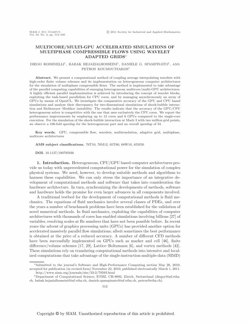


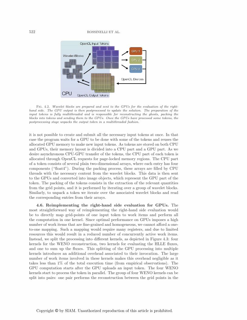


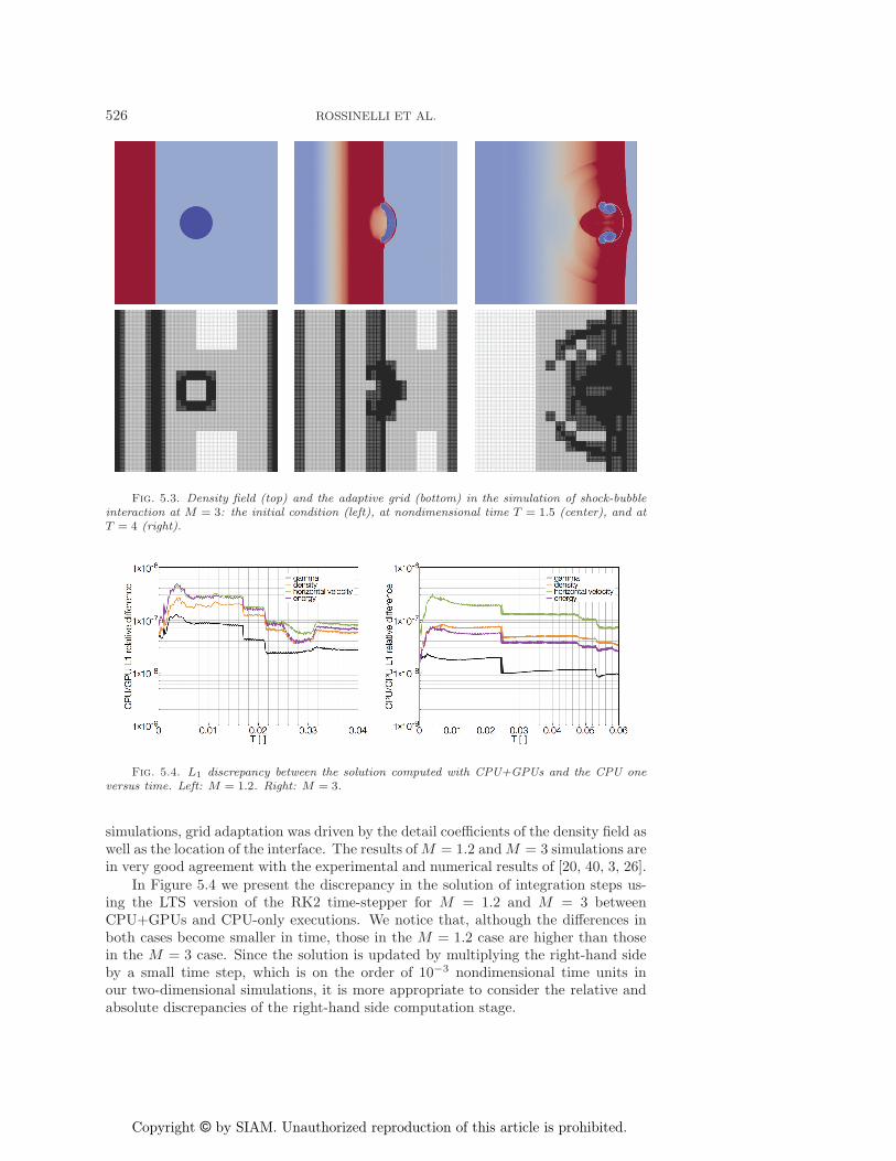


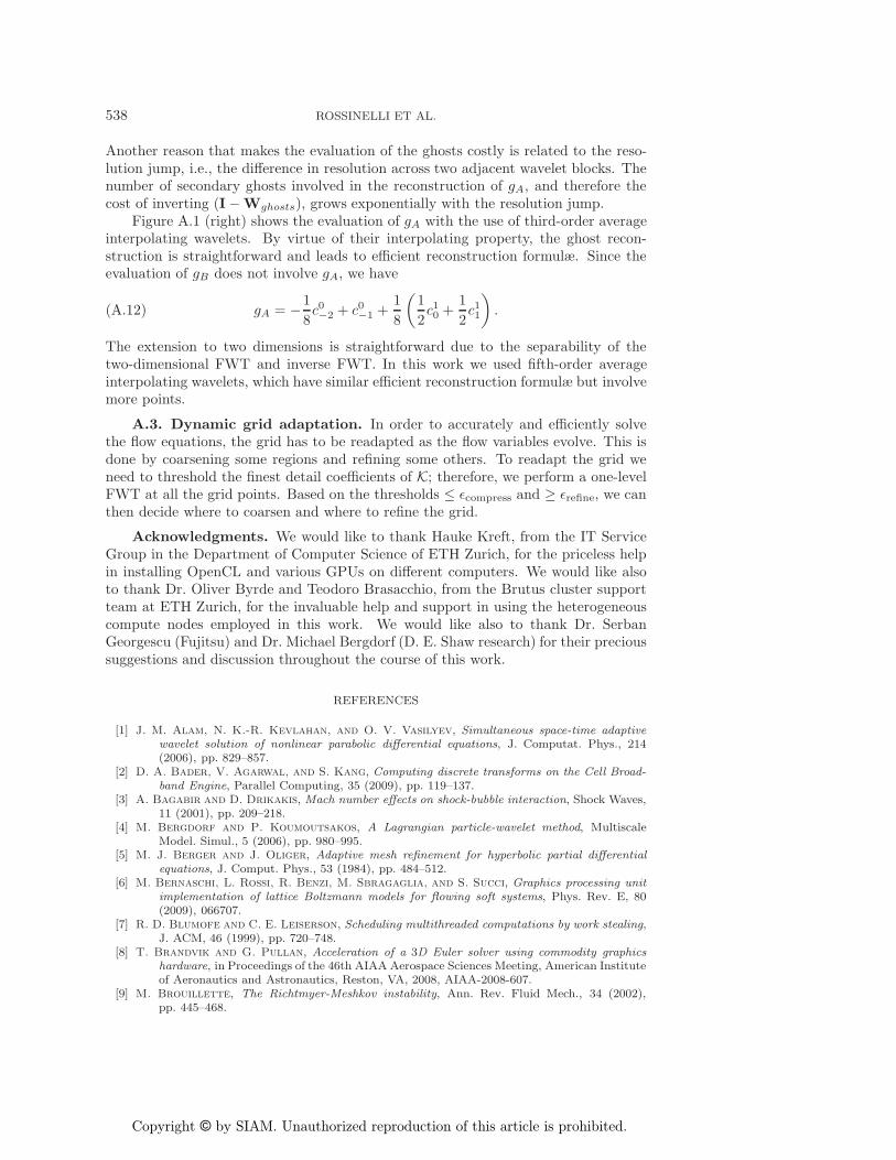


![SIAM J. S COMPUT cpeople.math.sfu.ca/~jfwillia/Research/Papers/BuddWilliamsSISC2009.pdf · the gradient flow of a variational principle [36], the condition that the curl (with respect](https://static.documents.pub/doc/80x56/5e7a1729a229ac7adb342b9c/siam-j-s-comput-jfwilliaresearchpapersbuddwilliamssisc2009pdf-the-gradient.jpg)


