Sigma-Point Kalman Filters for ProbabilisticInference in Dynamic State-Space Models

Rudolph van der Merwe & Eric WanOGI School of Science & EngineeringOregon Health & Science University

Beaverton, Oregon, 97006, USA{ rvdmerwe,ericwan}@ece.ogi.edu

Abstract

Probabilistic inference is the problem of estimating the hidden states ofa system in an optimal and consistent fashion given a set of noisy or in-complete observations. The optimal solution to this problem is given bythe recursive Bayesian estimation algorithm which recursively updatesthe posterior density of the system state as new observations arrive on-line. This posterior density constitutes the complete solution to the prob-abilistic inference problem, and allows us to calculate any "optimal" esti-mate of the state. Unfortunately, for most real-world problems, the opti-mal Bayesian recursion is intractable and approximate solutions must beused. Within the space of approximate solutions, the extended Kalmanfilter (EKF) has become one of the most widely used algorithms withapplications in state, parameter and dual estimation. Unfortunately, theEKF is based on a sub-optimal implementation of the recursive Bayesianestimation framework applied to Gaussian random variables. This canseriously affect the accuracy or even lead to divergence of any inferencesystem that is based on the EKF or that uses the EKF as a componentpart. Recently a number of related novel, more accurate and theoreti-cally better motivated algorithmic alternatives to the EKF have surfacedin the literature, with specific application to state estimation for auto-matic control. We have since generalized these algorithms, all based onderivativelessstatistical linearization,to a family of filters calledSigma-Point Kalman Filters(SPKF) and successfully expanded their use withinthe general field of probabilistic inference, both as stand-alone filters andas subcomponents of more powerful sequential Monte Carlo filters (parti-cle filters). We have consistently shown that there are large performancebenefits to be gained by applying Sigma-Point Kalman filters to areaswhere EKFs have been used as the de facto standard in the past, as wellas in new areas where the use of the EKF is impossible. This paper is asummary of that work that has appeared in a number of separate publi-cations as well as a presentation of some new results that has not beenpublished yet.

1 Introduction

Sequential probabilistic inference (SPI) is the problem of estimating the hidden states ofa system in an optimal and consistent fashion as set of noisy or incomplete observationsbecomes available online. Examples of this include vehicle navigation and tracking, time-series estimation and system identification or parameter estimation, to name but a few.This paper focuses specifically on discrete-time nonlinear dynamic systems that can be de-scribed by adynamic state-space model(DSSM) as depicted in Figure 1. The hidden sys-tem statexk, with initial distributionp(x0), evolves over time (k is the discrete time index)as an indirect or partially observed first order Markov process according to the conditionalprobability densityp(xk|xk−1). The observationsyk are conditionally independent giventhe state and are generated according to the probability densityp(yk|xk). The DSSM canalso be written as a set of nonlinear system equations

xk = f(xk−1,vk−1,uk;W) (process equation) (1)

yk = h(xk,nk;W) (observation equation) (2)

wherevk is the process noise that drives the dynamic system through the nonlinear statetransition functionf , andnk is the observation or measurement noise corrupting the obser-vation of the state through the nonlinear observation functionh. The state transition densityp(xk|xk−1) is fully specified byf and the process noise distributionp(vk), whereash andthe observation noise distributionp(nk) fully specify the observation likelihoodp(yk|xk).The exogenous input to the system,uk is assumed known. Bothf and/orh are parameter-ized via the parameter vectorW.

In a Bayesian framework, the posterior filtering densityp(xk|Yk) of the state given all theobservationsYk = {y1,y2, . . . ,yk} constitutes the complete solution to the sequentialprobabilistic inference problem, and allows us to calculate any "optimal" estimate of thestate, such as theconditional meanxk = E [xk|Yk] =

∫xkp(xk|Yk)dxk. The optimal

method to recursively update the posterior density as new observations arrive is given by therecursive Bayesian estimationalgorithm. This approach first projects the previous posteriorp(xk−1|Yk−1) forward in time using the probabilistic process model, i.e.

p(xk|Yk−1) =∫

p(xk|xk−1)p(xk−1|Yk−1)dxk−1 (3)

and then incorporates the latest noisy measurement using the observation likelihood togenerate the updated posterior

p(xk|Yk) = Cp(yk|xk)p(xk|Yk−1). (4)

The normalizing factor is given by

C =(∫

p(yk|xk)p(xk|Yk−1)dxk

)−1

. (5)

��

kx1k −x2k −x

2k −y 1k −y ky

1( | )k kp −x x

( | )k kp y x

Unobserved

Observed

Figure 1:Dynamic state space model.

Although this is the optimal recursive solution, it is usually only tractable forlinear, Gaus-sian systems in which case the closed-form recursive solution of the Bayesian integralequations is the well knownKalman filter [20]. For most general real-world (nonlin-ear, non-Gaussian) systems however, the multi-dimensional integrals are intractable andapproximate solutions must be used. These include methods such asGaussian approxi-mations(extended Kalman filter [15, 10]),hybrid Gaussian methods(score function EKF[26], Gaussian sum filters [1]),direct and adaptive numerical integration(grid-based filters[33]), sequential Monte Carlo methods(particle filters [6, 24, 7]) andvariational methods(Bayesian mixture of factor analyzers [11]) to name but a few.

Off all these methods, theextended Kalman filter(EKF) has probably had the mostwidespread use in nonlinear estimation and inference over the last 20 years. It has beenapplied successfully to problems in all areas of probabilistic inference, including state es-timation, parameter estimation (machine learning) and dual estimation [29, 2, 15, 12, 10].Even newer, more powerful inference frameworks such assequential Monte Carlo methodssometimes makes use of extended Kalman filters as subcomponents [6]. Unfortunately, theEKF is based on a suboptimal implementation of the recursive Bayesian estimation frame-work applied to Gaussian random variables. This can seriously affect the accuracy or evenlead to divergence of any inference system that is based on the EKF or that uses the EKFas a component part.

2 Gaussian Approximations

If we make the basic assumption that the state, observation and noise terms can be modeledas Gaussian random variables (GRVs), then the Bayesian recursion can be greatly simpli-fied. In this case, only the conditional meanxk = E [xk|Yk] and covariancePxk

needto be maintained in order to recursively calculate the posterior densityp(xk|Yk), which,under these Gaussian assumptions, is itself a Gaussian distribution1. It is straightforwardto show [2, 10, 23] that this leads to the recursive estimation

xk = (prediction ofxk) +Kk · [yk − (prediction ofyk)] (6)

= x−k +Kk ·(yk − y−

k

)(7)

Pxk= P−

xk−KkPyk

KTk . (8)

While this is alinear recursion, we have not assumed linearity of the model. The optimalterms in this recursion are given by

x−k = E [f(xk−1,vk−1,uk)] (9)

y−k = E

[h(x−k ,nk)

](10)

Kk = E[(xk − x−k )(yk − y−

k )T]E

[(yk − y−

k )(yk − y−k )T

]−1(11)

= PxkykP−1

yk(12)

where the optimal prediction (i.e., prior mean at timek) of xk is written asx−k , and corre-sponds to the expectation (taken over the posterior distribution of the state at timek − 1)of a nonlinear function of the random variablesxk−1 andvk−1 (similar interpretation forthe optimal predictiony−

k , except the expectation is taken over the prior distribution ofthe state at timek). The optimal gain termKk is expressed as a function of the expectedcross-correlation matrix (covariance matrix) of the state prediction error and the observa-tion prediction error, and the expected auto-correlation matrix of the observation prediction

1Given a Gaussian posterior, all optimal estimates of the system state such as MMSE, ML andMAP estimates are equivalent to the mean of the Gaussian density modeling the posterior.

error2. Note that evaluation of the covariance terms also require taking expectations of anonlinear function of the prior state variable.

2.1 The EKF and its flaws

The celebrated Kalman filter [20] calculates all terms in these equations exactly in the linearcase, and can be viewed as an efficient method for analytically propagating a GRV throughlinear system dynamics. For nonlinear models, however, theextended Kalman filter(EKF)must be used that first linearizes the system equations through a Taylor-series expansionaround the mean of the relevant Gaussian RV, i.e.

y = g(x) = g(x + δx)

= g(x) + ∇gδx +12∇2gδ2

x +13!

∇3gδ3x + . . . (13)

where the zero mean random variableδx has the same covariance,Px, asx. The mean andcovariance used in the EKF is thus obtained by taking the first-order truncated expectedvalue of Equation 13 (for the mean) and its outer-product (for the covariance), i.e.y ≈g(x), andPLIN

y = ∇gPx(∇g)T . Applying this result to Equations 6 and 8, we obtain,

x−k ≈ f(xk−1, v,uk) (14)

y−k ≈ h(x−k , n) (15)

Kk ≈ PLIN

xkyk

(PLIN

yk

)−1

. (16)

In other words, the EKF approximates the state distribution by a GRV, which is then prop-agated analytically through the “first-order” linearization of the nonlinear system. For theexplicit equations for the EKF see [15]. As such, the EKF can be viewed as providing“first-order” approximations to the optimal terms3. Furthermore, the EKF does not takeinto account the “uncertainty” in the underlying random variable when the relevant sys-tem equations are linearized. This is due to the nature of the first-order Taylor serieslinearization that expands the nonlinear equations around asingle pointonly, disregard-ing the “spread” (uncertainty) of the prior RV. These approximations and can introducelarge errors in the true posterior mean and covariance of the transformed (Gaussian) ran-dom variable, which may lead to suboptimal performance and sometimes divergence of thefilter [45, 43, 44].

3 Sigma-Point Kalman Filters (SPKF)

In order to improve the accuracy, consistency and efficiency4 of Gaussian approximate in-ference algorithms applied to general nonlinear DSSMs, the two major shortcomings ofthe EKF need to be addressed. These are: 1) Disregard for the “probabilistic spread” ofthe underlying system state and noise RVs during the linearization of the system equations,and 2) Limitedfirst-order accuracyof propagated means and covariances resulting froma first-order truncated Taylor-series linearization method. A number of related algorithms[16, 31, 14] have recently been proposed that address these issues by making use of novel

2The error between the true observation and the predicted observation,yk = yk − y−k is calledthe innovation.

3While “second-order” versions of the EKF exist, their increased implementation and computa-tional complexity tend to prohibit their use.

4Theaccuracyof an estimator is an indication of the average magnitude (taken over the distribu-tion of the data) of the estimation error. An estimator isconsistentif trace[Px] ≥ trace[Px] and itis efficientif that lower bound on the state error covariance is tight.

deterministic sampling approaches that circumvent the need to calculate analytical deriva-tives (such as the Jacobians of the system equations as needed by the EKF). It turns outthat these algorithms, collectively calledSigma-Point Kalman Filters (SPKFs) are re-lated through the implicit use of a technique calledweighted statistical linear regression5

[22] to calculate the optimal terms in the Kalman update rule (Equation 6).

3.1 Weighted statistical linear regression of a nonlinear function

Weighted statistical linear regression (WSLR) provides a solution to the problem of lin-earizing a nonlinear function of a random variable (RV), which takes into account the actualuncertainty (probabilistic spread) of that RV. In stead of linearizing the nonlinear functionthrough a truncated Taylor-series expansion at asinglepoint (usually taken to be the meanvalue of the RV), we rather linearize the function through a linear regression betweenrpoints drawn from the prior distribution of the RV, and thetruenonlinear functional evalu-ations of those points. Since this statistical approximation technique takes into account thestatistical properties of the prior RV the resultingexpectedlinearization error tends to besmaller than that of a truncated Taylor-series linearization.

In other words, consider a nonlinear functiony = g(x) which is evaluated inr points(X i,Yi) whereYi = g(X i). Define

x =r∑

i=1

wiX i (17)

Pxx =r∑

i=1

wi(X i − x)(X i − x)T (18)

y =r∑

i=1

wiYi (19)

Pyy =r∑

i=1

wi(Yi − y)(Yi − y)T (20)

Pxy =r∑

i=1

wi(X i − x)(Yi − y)T (21)

wherewi is a set ofr scalar regression weights such that∑r

i=1 wi = 1. Now, the aim isto find the linear regressiony = Ax + b that minimizes a statistical cost-function of theform J = E [φ(ei)], where the expectation is taken overi and hence the distribution of thex. The point-wise linearization error is given byei = Yi − (AX i + b), with covariancePee = Pyy −APxxAT , and the error functionalφ is usually taken to be the vector dotproduct. This reduces the cost function to the well known sum-of-squared-errors and theresulting minimization to

{A,b} = argminr∑

i=1

(wieieTi ) (22)

which has the following solution [10]

A = PTxyP

−1xx b = y −Ax. (23)

Given this statistically better motivated “linearization” method for a nonlinear function of aRV, how do we actually choose the number of and the specific location of these regression

5This technique is also known asstatistical linearization[10].

pointsX i, calledsigma-points,as well as their corresponding regression weights,wi? It isthe answer to this question that differentiate the different SPKF variants from each other.The next section gives a concise summary of these different approaches.

A simple example showing the superiority of the sigma-point approach is shown in Fig-ure 2 for a 2-dimensional system: the left plot shows the true mean and covariance propa-gation using Monte-Carlo sampling; the center plots show the results using a linearizationapproach as would be done in the EKF; the right plots show the performance of the sigma-point approach (note only 5 sigma points are required). The superior performance of thesigma-point approach is clear. The sigma-point approach results in approximations thatare accurate to the third order for Gaussian inputs for all nonlinearities and at least to thesecond order for non-Gaussian inputs. Another benefit of the sigma-point approach overthe EKF is that no analytical derivative need to be calculated. Only point-wise evaluationsof the system equations are needed which makes the SPKF ideally suited for estimation in“black box” systems.

3.2 SPKF Family : UKF, CDKF, SR-UKF & SR-CDKF

The Unscented Kalman Filter (UKF)

The UKF [16] is a SPKF that derives the location of the sigma-points as well as theircorresponding weights according to the following rationale [17]:The sigma-points shouldbe chosen so that they capture the most important statistical properties of the prior randomvariable x. This is achieved by choosing the points according to a constraint equationof the formξ (〈X , w〉 , r, p(x)) = 0, where〈X , w〉 is the set of all sigma-pointsX i andweightswi for i = 1, . . . r. It is possible to satisfy such a constraint condition and stillhave some degree of freedom in the choice of the point locations, by minimizing a furtherpenalty or cost-function of the formc (〈X , w〉 , r, p(x)). The purpose of this cost-functionis to incorporate statistical features ofx which are desirable, but do not necessarily haveto be met. In other words, the sigma-points are given by the solution to the followingoptimization problem

min〈X ,w〉

c (〈X , w〉 , r, p(x)) subject to ξ (〈X ,w〉 , r,p(x)) = 0 . (24)

The necessarystatistical information captured by the UKF is the first and second ordermoments ofp(x). The number6 of sigma-points needed to do thisr = 2L + 1 whereL isthe dimension ofx. It can be shown [18] that matching the moments ofx accurately upto thenth order means that Equations 19 and 20 capturey andPyy accurately up thenthorder as well. See [18, 44, 45] for more detail on how the sigma-points are calculated asa solution to Equation 24). The resulting set of sigma-points and weights utilized by theUKF is,

X 0 = x w(m)0 = λ

L+λ

X i = x +(√

(L + λ)Px

)i

i=1,...,L w(c)0 = λ

L+λ + (1−α2+β)

X i = x−(√

(L + λ)Px

)i

i=L+1,...,2L w(m)i = w

(c)i = 1

2(L+λ) i=1,...,2L

(25)whereλ = α2(L + κ) − L is a scaling parameter.α determines the spread of the sigmapoints aroundx and is usually set to a small positive value (e.g.1e − 2 ≤ α ≤ 1). κis a secondary scaling parameter which is usually set to either0 or 3 − L (see [45] fordetails), andβ is an extra degree of freedom scalar parameter used to incorporate any extraprior knowledge of the distribution ofx (for Gaussian distributions,β = 2 is optimal).

6By using a larger number of sigma-points higher order moments such as theskewor kurtosiscanalso be captured. See [17] for detail.

����� �������

��� ��� �������� ������� �!���#"!$

%'&)(*,+

-/.1032546-/.8769

:<;>= ?A@!BC;ED

Actual (sampling) Linearized (EKF)

sigma points

true mean

SP mean

and covarianceweighted sample mean

mean

SP covariance

covariance

true covariance

transformedsigma points

Sigma−Point

Figure 2: Example of the sigma-point approach for mean and covariance propagation. a)actual, b) first-order linearization (EKF), c) sigma-point approach.

(√(L + λ)Px

)i

is the ith row (or column) of the weighted matrix square root7 of the

covariancePx. See [44, 45] for precise implementational detail for the UKF.

The Central Difference Kalman Filter (CDKF)

Separately from the development of the UKF, two different groups [34, 14] proposed an-other SPKF implementation based onSterling’s interpolation formula.This formulationwas derived by replacing the analytically derived 1st and 2nd order derivatives in the Tay-lor series expansion (Equation 13) by numerically evaluatedcentral divided differences,i.e.

∇g ≈ g(x + hδx)− g(x− hδx)2h

(26)

∇2g ≈ g(x + hδx) + g(x− hδx)− 2g(x)h2

. (27)

Even though this approach is not explicitly derived starting from the statistical linear re-gression rationale, it can be shown [22] that the resulting Kalman filter again implicitlyemploys WSLR based linearization. The resulting set of sigma-points for the CDKF isonce again2L + 1points deterministically drawn from the prior statistics ofx, i.e.

X 0 = x w0 = h2−Lh2

X i = x +(√

h2Px

)i

i=1,...,L wi = 12h2 i=1,...,2L

X i = x−(√

h2Px

)i

i=L+1,...,2L

For exact implementation details of the CDKF algorithm, see [30, 39, 45]. It is shownin [31] that the CDKF has marginally higher theoretical accuracy than the UKF in the

7We typically use the numerically efficientCholesky factorizationmethod to calculate the matrixsquare root.

higher order terms of the Taylor series expansion, but we’ve found in practice that allSPKFs (CDKF and UKF) perform equally well with negligible difference in estimationaccuracy. Both generate estimates however that are clearly superior to those calculated byan EKF. One advantage of the CDKF over the UKF is that it only uses a single scalar scalingparameter, the central difference half-step sizeh, as opposed to the three (α, κ, β)that theUKF uses. Once again this parameter determines thespreadof the sigma-points aroundthe prior mean. For Gaussian priors, its optimal value is

√3 [31].

Square-root Forms (SR-UKF, SR-CDKF)

One of the most costly operations in the SPKF is the calculation of the matrix square-root of the state covariance at each time step in order to form the sigma-point set. Due tothis and the need for more numerical stability (especially during the state covariance up-date), we derived numerically efficientsquare-rootforms of both the UKF and the CDKF[39, 40]. These forms propagate and update the square-root of the state covariance directlyin Cholesky factored form, using the sigma-point approach the following three powerfullinear algebra techniques:QR decomposition, Cholesky factor updatingandefficient pivot-based least squares. For implementation details, see [45, 39, 40]. The square-root SPKFs(SR-UKF and SR-CDKF) has equal (or marginally better) estimation accuracy when com-pared to the standard SPKF, but at the added benefit of reduced computational cost forcertain DSSMs and a consistently increased numerical stability. For this reason, they areour preferred form for SPKF use in stand-alone estimators as well as in SMC/SPKF hybrids(see Section 5).

4 Experimental Results : SPKF applied to state, parameter and dualestimation

4.1 State Estimation

The UKF was originally designed for state estimation applied to nonlinear control appli-cations requiring full-state feedback [16, 18, 19]. We provide a new application examplecorresponding to noisy time-series estimation with neural networks. For further examples,see [45].

Noisy time-series estimation: In this example, a SPKF (UKF) is used to estimate anunderlying clean time-series corrupted by additive Gaussian white noise. The time-seriesused is the Mackey-Glass-30 chaotic series [25, 21]. The clean times-series is first modeledas a nonlinear autoregression

xk = f(xk−1, xk−2, . . . , xk−M ;w) + vk (28)

where the modelf (parameterized byw) was approximated by training a feedforwardneural network on the clean sequence. The residual error after convergence was taken tobe the process noise variance. Next, white Gaussian noise was added to the clean Mackey-Glass series to generate a noisy time-seriesyk = xk + nk. In the estimation problem, thenoisy-time seriesyk is the only observed input to either the EKF or SPKF algorithms (bothutilize the known neural network model). Note that for time-series estimation, both theEKF and the SPKF areO(L2) complexity. Figure 3 shows a sub-segment of the estimatesgenerated by both the EKF and the SPKF (the original noisy time-series has a 3dB SNR).The superior performance of the SPKF is clearly visible.

4.2 Parameter Estimation

The classic machine learning problem involves determining a nonlinear mapping

yk = g(xk,w) (29)

200 210 220 230 240 250 260 270 280 290 300−5

0

5

kx(

k)

Estimation of Mackey−Glass time series : EKF

cleannoisyEKF

200 210 220 230 240 250 260 270 280 290 300−5

0

5

k

x(k)

Estimation of Mackey−Glass time series : UKF

cleannoisyUKF

Figure 3: Estimation of Mackey-Glass time-series with the EKF and SPKF using a knownmodel. Bottom graph shows comparison of estimation errors for complete sequence.

wherexk is the input,yk is the output, and the nonlinear mapg is parameterized by thevectorw. The nonlinear map, for example, may be a feed-forward or recurrent neuralnetwork (w are the weights), with numerous applications in regression, classification, anddynamic modeling. It can also be a general nonlinear parametric model, such as the dy-namic/kinematic vehicle model, parameterized by a finite set of coefficients . Learningcorresponds to estimating the parametersw. Typically, a training set is provided with sam-ple pairs consisting of known input and desired outputs,{xk,dk}. The error of the machineis defined asek = dk − g(xk,w), and the goal of learning involves solving for the param-etersw in order to minimize the expectation of some function of this error (typically theexpected square error). Note that in contrast to state (and dual) estimation, the input is usu-ally observed noise-free and does not require estimation. While a number of optimizationapproaches exist (e.g., gradient descent), the SPKF may be used to estimate the parametersby writing a new state-space representation

wk = wk−1 + vk

yk = g(xk,wk) + ek (30)

where the parameterswk correspond to a stationary process with identity state transitionmatrix, driven by process noisevk (the choice of variance determines tracking perfor-mance). The outputyk corresponds to a nonlinear observation onwk. The SPKF can thenbe applied directly as an efficient “second-order” technique for learning the parameters.

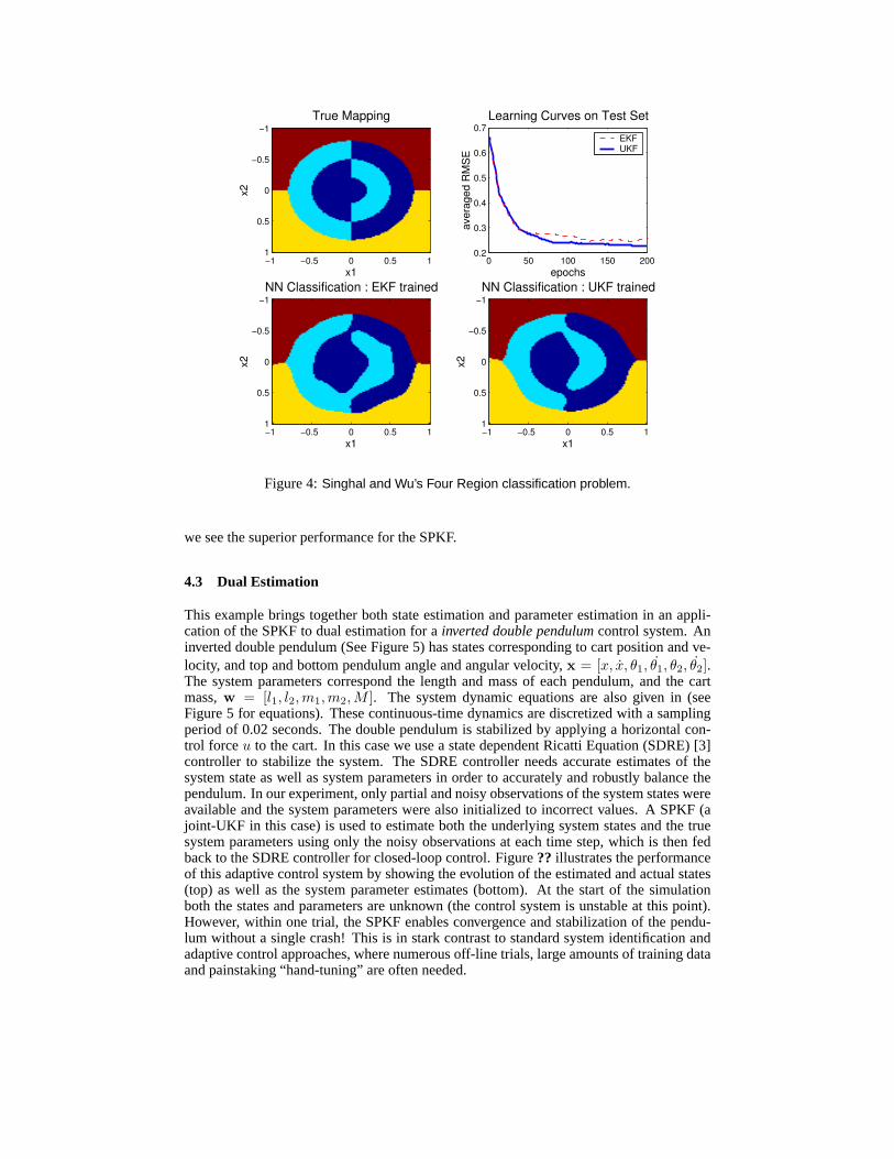
Four Regions Classification: In the parameter estimation example, we consider a bench-mark pattern classification problem having four interlocking regions [37]. A three-layerfeedforward network (MLP) with 2-10-10-4 nodes is trained using inputs randomly drawnwithin the pattern space,S = [−1, 1] × [1, 1], with the desired output value of+0.8 if thepattern fell within the assigned region and−0.8 otherwise. Figure 4 illustrates the clas-sification task, learning curves for the SPKF (UKF) and EKF, and the final classificationregions. For the learning curve, each epoch represents 100 randomly drawn input samples.The test set evaluated on each epoch corresponds to a uniform grid of 10,000 points. Again,

x1

x2

True Mapping

−1 −0.5 0 0.5 1

−1

−0.5

0

0.5

1

x1

x2

NN Classification : EKF trained

−1 −0.5 0 0.5 1

−1

−0.5

0

0.5

1

x1

x2

NN Classification : UKF trained

−1 −0.5 0 0.5 1

−1

−0.5

0

0.5

1

0 50 100 150 2000.2

0.3

0.4

0.5

0.6

0.7Learning Curves on Test Set

epochs

aver

aged

RM

SE

EKFUKF

Figure 4:Singhal and Wu’s Four Region classification problem.

we see the superior performance for the SPKF.

4.3 Dual Estimation

This example brings together both state estimation and parameter estimation in an appli-cation of the SPKF to dual estimation for ainverted double pendulumcontrol system. Aninverted double pendulum (See Figure 5) has states corresponding to cart position and ve-locity, and top and bottom pendulum angle and angular velocity,x = [x, x, θ1, θ1, θ2, θ2].The system parameters correspond the length and mass of each pendulum, and the cartmass,w = [l1, l2,m1,m2,M ]. The system dynamic equations are also given in (seeFigure 5 for equations). These continuous-time dynamics are discretized with a samplingperiod of 0.02 seconds. The double pendulum is stabilized by applying a horizontal con-trol forceu to the cart. In this case we use a state dependent Ricatti Equation (SDRE) [3]controller to stabilize the system. The SDRE controller needs accurate estimates of thesystem state as well as system parameters in order to accurately and robustly balance thependulum. In our experiment, only partial and noisy observations of the system states wereavailable and the system parameters were also initialized to incorrect values. A SPKF (ajoint-UKF in this case) is used to estimate both the underlying system states and the truesystem parameters using only the noisy observations at each time step, which is then fedback to the SDRE controller for closed-loop control. Figure?? illustrates the performanceof this adaptive control system by showing the evolution of the estimated and actual states(top) as well as the system parameter estimates (bottom). At the start of the simulationboth the states and parameters are unknown (the control system is unstable at this point).However, within one trial, the SPKF enables convergence and stabilization of the pendu-lum without a single crash! This is in stark contrast to standard system identification andadaptive control approaches, where numerous off-line trials, large amounts of training dataand painstaking “hand-tuning” are often needed.

1 2 1 2 1 1 1 2 1 2 2

2 2

1 2 1 1 1 2 2 2 2

211 2 1 1 2 1 1 2 1 2 2 2

2

1 2 1 1 2 1 2 2 2 1

2 2 2 2 1 2

( ) ( 2 ) cos cos

( 2 ) sin sin

( 2 ) cos 4( ) 2 sin3

( 2 ) sin 2 sin( )

sin 2 cos(

M m m x m m l m l

u m m l m l

mm m l x m l m l l

m m gl m l l

m xl m l l 2

2 1 2 2 2

2

2 2 2 2 1 2 1 2 1

4)3

sin 2 sin( )

m l

m gl m l l

xuSDRE

controller

Parameter Est.

SPKF

u

n

x

u

x

1

22 2,l m

1 1,l m

M

( )kA x

State Est.

Sensor noise

1 2 1 2 1 1 1 2 1 2 2

2 2

1 2 1 1 1 2 2 2 2

211 2 1 1 2 1 1 2 1 2 2 2

2

1 2 1 1 2 1 2 2 2 1

2 2 2 2 1 2

( ) ( 2 ) cos cos

( 2 ) sin sin

( 2 ) cos 4( ) 2 sin3

( 2 ) sin 2 sin( )

sin 2 cos(

M m m x m m l m l

u m m l m l

mm m l x m l m l l

m m gl m l l

m xl m l l 2

2 1 2 2 2

2

2 2 2 2 1 2 1 2 1

4)3

sin 2 sin( )

m l

m gl m l l

xuSDRE

controller

Parameter Est.

SPKF

u

n

x

u

x

1

22 2,l m

1 1,l m

Mu

x

1

22 2,l m

1 1,l m

Mu

x

1

22 2,l m

1 1,l m

M

( )kA x

State Est.

Sensor noise

0 50 100 150 200−1

−0.8

−0.6

−0.4

−0.2

0

0.2

0.4

0.6

time

stat

e es

timat

es

angle 1

angle 2

true states noisy observationsUKF estimates

0 50 100 150 2000.2

0.4

0.6

0.8

1

1.2

1.4

1.6

1.8

time

para

met

ers

estim

ates cart mass

pendulum 1 length & mass

pendulum 2 length & mass

true model parametersUKF estimates

Figure 5: Inverted double pendulum dual estimation and control experiment. Dynamicmodel and schematic of control system (top plot). Estimation results are shown in the bottomplot: state estimates (top) and parameter estimates(bottom).

5 Sequential Monte Carlo / SPKF Hybrids

The SPKF, like the EKF, still assumes a Gaussian posterior which can fail in certain non-linear non-Gaussian problems with multi-modal and/or heavy tailed posterior distributions.The Gaussian sum filter (GSF) addresses this issue by approximating the posterior densitywith a finite Gaussian mixture and can be interpreted as a parallel bank of EKFs. Unfor-tunately, due to the use of the EKF as a subcomponent, it also suffers from similar short-comings as the EKF. Recently, particle based sampling filters have been proposed and usedsuccessfully to recursively update the posterior distribution usingsequential importancesampling and resampling[7]. These methods (collectively calledparticle filters) approx-imate the posterior by a set of weighted samples without making any explicit assumptionabout its form and can thus be used in general nonlinear, non-Gaussian systems. In thissection, we present hybrid methods that utilizes the SPKF to augment and improve thestandard particle filter, specifically through generation of theimportance proposal distri-butions. We will briefly review only the background fundamentals necessary to introduce

particle filtering and then discuss the two extensions based on the SPKF, theSigma-PointParticle Filter (SPPF) and theGaussian-Mixture Sigma-Point Particle Filter(GMSPPF).

5.1 Particle Filters

Theparticle filter is a sequential Monte Carlo (SMC) based method that allows for a com-plete representation of the state distribution using sequential importance sampling and re-sampling [6, 24]. Whereas the standard EKF and SPKF make a Gaussian assumption tosimplify the optimal recursive Bayesian estimation, particle filters make no assumptions onthe form of the probability densities in question, i.e, full nonlinear, non-Gaussian estima-tion.

Monte Carlo simulation and sequential importance sampling

Particle filtering is based on Monte Carlo simulation with sequential importance sampling(SIS). The overall goal is to directly implement optimal Bayesian estimation by recursivelyapproximating the complete posterior state density. Importance sampling is a Monte-Carlomethod that represents a distributionp(x) by an empirical approximation based on a setof weighted samples (particles), i.e.p(x) ≈ p(x) =

∑Ni=1 w(i)δ(x − x(i)), whereδ(.) is

the Dirac delta function, and the weighted sample set, {w(l),x(i); l = 1 . . . N } are drawnfrom some related, easy-to-sample-fromproposaldistributionπ(x). The weights are given

by w(i) = p(x(i))/π(x(i))∑Ni=1 p(x(i))/π(x(i))

. Given this, any estimate of the system such asEp[g(x)] =∫g(x)p(x)dx can be approximated byE[g(x)] =

∑Ni=1 w(i)g(X (i)) [7]. Using the first

order Markov nature of our DSSM and the conditional independence of the observationsgiven the state, a recursive update formula (implicitly a nonlinear measurement update) forthe importance weights can be derived [7]. This is given by

w(i)k = w

(i)k−1p(yk|xk)p(xk|xk−1)/π(xk|Xk−1,Yk) for xk = x(i). (31)

Equation (31) provides a mechanism to sequentially update the importance weights givenan appropriate choice of proposal distribution,π(xk|Xk−1,Yk). Since we can samplefrom the proposal distribution and evaluate the likelihoodp(yk|xk) and transition prob-abilities p(xk|xk−1), all we need to do is generate a prior set of samples and iterativelycompute the importance weights. This procedure then allows us to evaluate the expecta-tions of interest by the following estimate

E [g(xk)] ≈1/N

∑Ni=1 w

(i)k g(x(i)

k )

1/N∑N

i=1 w(i)k

=N∑

i=1

w(i)k g(x(i)

k ) (32)

where the normalized importance weightsw(i)k = w

(i)k /

∑Nj=1 w

(j)k . This estimate asymp-

totically converges if the expectation and variance ofg(xk) andwk exist and are bounded,and if the support of the proposal distribution includes the support of the posterior distri-bution. Thus, asN tends to infinity, the posterior filtering density function can be approxi-mated arbitrarily well by the point-mass estimate

p(xk|Yk) =N∑

i=1

w(i)k δ(xk − x

(i)k )

These point-mass estimates can approximate any general distribution arbitrarily well, lim-ited only by the number of particles used and how well the above mentioned importancesampling conditions are met.

sampling

Index

i

j resampled index p(i)

cdf

1

( )jtw�

1N −

Figure 6:Resampling process, whereby a random measure {x(i)k , w

(i)k } is mapped into an

equally weighted random measure {x(j)k , N−1}. The index i is drawn from a uniform distri-

bution.

Resampling and Sample Depletion

The sequential importance sampling (SIS) algorithm discussed so far has a serious limita-tion: the variance of the importance weights increases stochastically over time. Typically,after a few iterations, one of the normalized importance weights tends to 1, while the re-maining weights tend to zero. A large number of samples are thus effectively removedfrom the sample set because their importance weights become numerically insignificant.To avoid this degeneracy, a resampling or selection stage may be used to eliminate sampleswith low importance weights and multiply samples with high importance weights. We typ-ically make use of eithersampling-importance resampling(SIR) or residual resampling.See [7] for more theoretical and implementational detail on resampling.

After the selection/resampling step at timek, we obtainN particles distributed marginallyapproximately according to the posterior distribution. Since the selection step favors thecreation of multiple copies of the “fittest” particles, many particles may end up having nochildren (Ni = 0), whereas others might end up having a large number of children, theextreme case beingNi = N for a particular valuei. In this case, there is a severe depletionof samples. Therefore, and additional procedure, such as a single MCMC step, is oftenrequired to introduce sample variety after the selection step without affecting the validityof the approximation they infer. See [42] for more detail.

The Particle Filter Algorithm

The pseudo-code of a generic particle filter is presented in Algorithm 1. In implementingthis algorithm, the choice of the proposal distributionπ(xk|Xk−1,Yk) is the most criti-cal design issue. The optimal proposal distribution (which minimizes the variance on theimportance weights) is given by [6, 24],

π(xk|Xk−1,Yk) = p(xk|Xk−1,Yk)

i.e., the true conditional state density given the previous state history and all observations.Sampling from this is, of course, impractical for arbitrary densities (recall the motivationfor using importance sampling in the first place). Consequently the transition prior is themost popular choice of proposal distribution [7]8,

π(xk|Xk−1,Yk) $ p(xk|xk−1).

For example, if an additive Gaussian process noise model is used, the transition prior issimply,

p(xk|xk−1) = N(xk; f(xk−1),Rv

k−1

). (33)

8The notation$ denotes“chosen as”, to indicate a subtle difference versus“approximation”.

Algorithm 1 Algorithm for the generic particle filter1. Initialization: k=0

• For i = 1, . . . , N , draw (sample) particlex(i)0 from the priorp(x0).

2. Fork = 1, 2, . . .

(a) Importance sampling step

• For i = 1, . . . , N , samplex(i)k ∼ π(xk|x(i)

k−1,Yk).• For i = 1, . . . , N , evaluate the importance weights up to a normalizing

constant:

w(i)k = w

(i)k−1

p(yk|x(i)k )p(x(i)

k |π(x(i)

k |x(i)k−1,Yk)

(34)

• For i = 1, . . . , N , normalize the importance weights:w(i)k =

w(i)k /

∑Nj=1 w

(j)k .

(b) Selection step (resampling)

• Multiply/suppress samplesx(i)k with high/low importance weightsw(i)

k ,respectively, to obtainN random samples approximately distributed ac-cording top(xk|Yk).

• For i = 1, . . . , N , setw(i)k = w

(i)k = N−1.

• (optional) Do a single MCMC (Markov chain Monte Carlo) move step toadd further ’variety’ to the particle set without changing their distribution.

(c) Output:The output of the algorithm is a set of samples that can be used to ap-proximate the posterior distribution as follows:p(xk|Yk) = 1

N

∑Ni=1 δ(xk−

x(i)k ). From these samples, any estimate of the system state can be calculated,

such as the MMSE estimate,

xk = E [xk|Yk] ≈ 1N

N∑i=1

x(i)k .

Similar expectations of the functiong(xk) (such as MAP estimate, covari-ance, skewness, etc.) can be calculated as a sample average.

The effectiveness of this approximation depends on how close the proposal distribution isto the true posterior distribution. If there is not sufficient overlap, only a few particles willhave significant importance weights when their likelihood are evaluated.

5.2 The Sigma-Point Particle Filter

An improvement in the choice of proposal distribution over the simple transition prior,which also address the problem of sample depletion, can be accomplished by moving theparticles towards the regions of high likelihood, based on the most recent observationyk

(See Figure 7).

An effective approach to accomplish this, is to use an EKF generated Gaussian approxima-tion to the optimal proposal, i.e,

π(xk|xk−1,Yk) $ qN (xk|Yk),

which is accomplished by using a separate EKF to generate and propagate a Gaussian

.LikelihoodPrior

Figure 7:Including the most current observation into the proposal distribution, allows us tomove the samples in the prior to regions of high likelihood. This is of paramount importanceif the likelihood happens to lie in one of the tails of the prior distribution, or if it is too narrow(low measurement error).

proposal distribution for each particle, i.e.,

qN (xk|Yk) = N(xk;x(i)

k ,P(i)k

)i = 1, 2, . . . N (35)

That is, at timek one uses the EKF equations, with the new data, to compute the meanand covariance of the importance distribution for each particle from the previous time stepk − 1. Next, we redraw thei-th particle (at timek) from this new updated distribution.While still making a Gaussian assumption, the approach provides a better approximation tothe optimal conditional proposal distribution and has been shown to improve performanceon a number of applications [5].

By replacing the EKF with a SPKF9, we can more accurately propagate the mean andcovariance of the Gaussian approximation to the state distribution. Distributions generatedby the SPKF will have a greater support overlap with the true posterior distribution thanthe overlap achieved by the EKF estimates. In addition, scaling parameters used for sigmapoint selection can be optimized to capture certain characteristic of the prior distributionif known, i.e., the algorithm can be modified to work with distributions that have heaviertails than Gaussian distributions such as Cauchy or Student-t distributions. The new filterthat results from using a SPKF for proposal distribution generation within a particle filterframework is called theSigma-Point Particle Filter(SPPF). Referring to Algorithm 1 forthe generic particle filter, the first item in the importance sampling step:

• For i = 1, . . . , N , samplex(i)k ∼ π(xk|x(i)

k−1,Yk).

is replaced with the following SPKF update:

• For i = 1, . . . , N :

– Update the Gaussian prior distribution for each particle with the SPKF :

∗ Calculate sigma-points for particle,xa,(i)k−1 = [x(i)

k−1 vk−1 nk−1]T :

X a,(i)k−1,(0...2L) =

[x

a,(i)k−1 x

a,(i)k−1 + γ

√Pa,(i)

k−1 xa,(i)k−1 − γ

√Pa,(i)

k−1

]

9Specifically we make use of either aSquare-Root Unscented Kalman filter(SR-UKF) or aSquare-Root Central-Difference KalmanFilter (SR-CDKF).

∗ Propagate sigma-points into future (time update):

X x,(i)k|k−1,(0...2L) = f

(X x,(i)

k−1,(0...2L),Xv,(i)k−1,(0...2L),uk

)x

(i)k|k−1 =

2L∑j=0

w(m)j X x,(i)

k|k−1,j

P(i)k|k−1 =

2L∑j=0

w(c)j (X x,(i)

k|k−1,j − x(i)k|k−1)(X

x,(i)k|k−1,j − x

(i)k|k−1)

T

Y(i)k|k−1,(0...2L) = h

(X x,(i)

k|k−1,(0...2L),Xn,(i)k−1,(0...2L)

)y(i)

k|k−1 =2L∑j=0

W(m)j Y(i)

j,k|k−1

∗ Incorporate new observation (measurement update):

Pykyk=

2L∑j=0

w(c)j [Y(i)

k|k−1,j − y(i)k|k−1][Y

(i)k|k−1,j − y(i)

k|k−1]T

Pxkyk=

2L∑j=0

w(c)j [X (i)

k|k−1,j − x(i)k|k−1][Y

(i)k|k−1,j − y(i)

k|k−1]T

Kk = PxkykP−1

xkykx

(i)k = x

(i)k|k−1 + Kk(yk − y(i)

k|k−1)

P(i)k = P(i)

k|k−1 −KkPykykKT

k

– Samplex(i)k ∼ q(xk|xk−1,Yk) ≈ N

(xk; x(i)

k ,P(i)k

)All other steps in the particle filter formulation remain unchanged. The SPPF presentedabove makes use of a UKF for proposal generation. Our preferred form however, is a SPPFbased around the square-root CDKF (SR-CDKF) which has the numerical efficiency andstability benefits laid out in Section 3.2. The UKF was used in above in order to simplifythe presentation of the algorithm. For experimental verification of the superior estimationperformance of the SPPF over a standard particle filter, see Section 6. For more detail onthe SPPF, see [42, 38]10 .

5.3 Gaussian Mixture Sigma-Point Particle Filters

Particle filters need to use a large number of particles for accurate and robust operation,which often make their use computationally expensive. Furthermore, as pointed out ear-lier, they suffer from an ailment called “sample depletion” that can cause the sample basedposterior approximation to collapse over time to a few samples. In the SPPF section weshowed how this problem can be addressed by moving particles to areas of high likelihoodthrough the use of a SPKF generated proposal distribution. Although the SPPF has largeestimation performance benefits over the standard PF, it still incurs a heavy computationalburden since it has to run anO(mym2

x) SPKF for each particle in the posterior state distri-bution.

In this section we present a further refinement of the SPPF called theGaussian MixtureSigma-Point Particle Filter(GMSPPF) [41]. This filter has equal or better estimation per-formance when compared to standard particle filters and the SPPF, at a largely reduced

10The original name of the SPPF algorithm was theunscented particle filter(UPF).

computational cost. The GMSPPF combines animportance sampling(IS) based measure-ment update step with aSPKF based Gaussian sum filterfor the time-update and proposaldensity generation. The GMSPPF uses a finite Gaussian mixture model (GMM) representa-tion of the posterior filtering density, which is recovered from the weighted posterior parti-cle set of the IS based measurement update stage, by means of aExpectation-Maximization(EM) step. The EM step either follows directly after the resampling stage of the particlefilter, or it can completely replace that stage if aweighted EMalgorithm is used. The EM orWEM recovered GMM posterior further mitigates the “sample depletion” problem throughits inherent “kernel smoothing” nature. The three main algorithmic components used in theGMSPPF are briefly discussed below to provide some background on their use. Then weshow how these three components are combined to form the GMSPPF algorithm.

- SPKF based Gaussian mixture approximation

It can be shown [2] than any probability densityp(x) can be approximated as closely asdesired by a Gaussian mixture model (GMM) of the following form,p(x) ≈ pG(x) =∑G

g=1 α(g)N (x;µ(g),P(g)), whereG is the number of mixing components,α(g) are themixing weights andN (x;µ,P) is a normal distribution with mean vectorµ and positivedefinite covariance matrixP. Given Equations 1 and 2, and assuming that the prior densityp(xk−1|Yk−1) and system noise densitiesp(vk−1) andp(nk) are expressed by GMMs, thefollowing densities can also be approximated by GMMs: 1) thepredictive prior density,

p(xk|Yk−1)≈pG(xk|Yk−1) =∑G′

g′=1 α(g′)N (x; µ(g′)k , P(g′)

k ), and 2) theupdated poste-

rior density,p(xk|Yk)≈pG(xk|Yk) =∑G′′

g′′=1 α(g′′)N (x;µ(g′′)k ,P(g′′)

k ), whereG′ = GI

andG′′ = G′J = GIJ (G, I andJ are the number of components in the state, processnoise, and observation noise GMMs respectively). The predicted and updated Gaussiancomponent means and covariances ofpG(xk|Yk−1) andpG(xk|Yk) are calculated usingthe Kalman filter Equations 6 and 8 (In the GMSPPF we use a bank of SPKFs). The mix-ing weight update procedure are shown below in the algorithm pseudo-code. It is clear thatthe number of mixing components in the GMM representation grows fromG to G′ in thepredictive (time update) step and fromG′ to G′′ in the subsequent measurement updatestep. Over time, this will lead to an exponential increase in the total number of mixingcomponents and must be addressed by a mixing-component reduction scheme. See belowfor how this is achieved.

- Importance sampling (IS) based measurement update

In the GMSPPF we use the GMM approximatepG(xk|Yk) from the bank of SPKFs (seeabove) as the proposal distributionπ(xk). In Section 5.2 and [38] we showed that samplingfrom such a proposal (which incorporates the latest observation), moves particles to areasof high likelihood which in turn reduces the “sample depletion” problem. Furthermore weuse the predictive prior distributionpG(xk|Yk−1) (see Sec.5.3) as asmoothed(over priordistribution ofxk−1) evaluation of thep(xk|xk−1) term in the weight update equation.This is needed since the GMSPPF represents the posterior (which becomes the prior at thenext time step) by a GMM, which effectively smoothes the posterior particle set by a set ofGaussian kernels.

- EM/WEM for GMM recovery

The output of the IS-based measurement update stage is a set ofN weighted particles,which in the standard particle filter isresampledin order to discard particles with in-significant weights and multiply particles with large weights. The GMSPPF representsthe posterior by a GMM which is recovered from the resampled, equally weighted parti-cle set using a standardExpectation-Maximization(EM) algorithm, or directly from theweightedparticles using aweighted-EM(WEM) [27] step. Whether aresample-then-EMor adirect-WEMGMM recovery step is used depends on the particular nature of the infer-

ence problem at hand. It is shown in [7] that resampling is needed to keep the variance ofthe particle set from growing too rapidly . Unfortunately, resampling can also contribute tothe “particle depletion” problem in cases where the measurement likelihood is very peaked,causing the particle set to collapse to multiple copies of the same particle. In such a case,thedirect-WEMapproach might be preferred. On the other hand, we have found that forcertain problems where the disparity (as measured by the KL-divergence) between the trueposterior and the GMM-proposal is large, theresample-then-EMapproach performs better.This issue is still being investigated.

This GMM recovery step implicitly smoothes over the posterior set of samples, avoidingthe “particle depletion” problem, and at the same time the number of mixing componentsin the posterior is reduced toG, avoiding the exponential growth problem alluded to above.Alternatively, one can use a more powerful “clustering” approach that automatically triesto optimize the model order (i.e. number of Gaussian components) through the use of someprobabilistic cost function such as AIC or BIC [28, 32]. This adaptive approach allows forthe complexity of the posterior to change over time to better model the true nature of theunderlying process, although at an increased computational cost.

5.3.1 The GMSPPF Algorithm

The full GMSPPF algorithm will now be presented based on the component parts discussedabove.

A) Time update and proposal distribution generation

At time k-1, assume the posterior state density is approximated by theG-component GMM

pG(xk−1|Yk−1) =G∑

g=1

α(g)k−1N

(xk−1;µ

(g)k−1,P

(g)k−1

), (36)

and the process and observation noise densities are approximated by the followingI andJcomponent GMMs respectively

pG(vk−1) =I∑

i=1

β(i)k−1N

(vk−1;µv

(i)k−1,Q

(i)k−1

)(37)

pG(nk) =J∑

j=1

γ(j)k N

(nk;µn

(j)k ,R(j)

k

)(38)

Following the GSF approach of [1], but replacing the EKF with a SPKF, the output ofa bank ofG′′ = GIJ parallel SPKFs are used to calculate GMM approximations ofp(xk|Yk−1) andp(xk|Yk) according to the pseudo-code given below. For clarity of no-tation defineg′ = g + (i − 1)G and note that references tog′ implies references to therespectiveg andi, since they are uniquely mapped. Similarly defineg′′ = g′ + (j − 1)GIwith the same implied unique index mapping. Now,

1. For j=1 . . . J , set pj(nk) = N (nk;µ(j)n,k,R(j)

k ). For i=1 . . . I,

set pi(vk−1)=N (vk−1;µ(i)v,k−1,Q

(i)k−1) and for g=1 . . . G, set

pg(xk−1|Yk−1)=N (xk−1;µ(g)k−1,P

(g)k−1).

2. For g′=1 . . . G′ use the time update step of a SPKF11 (employing the systemprocess equation (1) and densitiespg(xk−1|Yk−1) andpi(vk−1) from above) to

11The SPKF algorithm pseudo-code will not be given here explicitly. See [45, 39] for implemen-tation details.

calculate a Gaussian approximatepg′(xk|Yk−1)=N (xk; µ(g′)k , P(g′)

k ) and update

the mixing weights,α(g′)k = α

(g)k−1β

(i)k−1/(

∑Gg=1

∑Ii=1 α

(g)k−1β

(i)k−1).

(a) Forg′′ = 1 . . . G′′, complete the measurement update step of each SPKF(employing the system observation equation (2), current observationyk, anddensitiespg′(xk|Yk−1) andpj(nk) from above) to calculate a Gaussian ap-

proximatepg′′(xk|Yk)=N (xk;µ(g′′)k ,P(g′′)

k ). Also update the GMM mix-

ing weights,α(g′′)k = α

(g′)k γ

(j)k S

(j)k /(

∑G′

g′=1

∑Jj=1 α

(g′)k γ

(j)k S

(j)k ), where

S(j)k = pj(yk|xk) evaluated atxk = µ

(g′)k for the current observation,yk.

The predictive state density is now approximated by the GMM

pG(xk|Yk−1) =G′∑

g′=1

α(g′)k N

(xk;µ(g′)

k , P(g′)k

)(39)

and the posterior state density (which will only be used as the proposal distribution in theIS-based measurement update step) is approximated by the GMM

pG(xk|Yk) =G′′∑

g′′=1

α(g′′)k N

(xk;µ(g′′)

k ,P(g′′)k

)(40)

B) Measurement update

1. DrawN samples {x(i)k ; l = 1 . . . N } from the proposal distributionpG(xk|Yk)

(Equation 40) and calculate their corresponding importance weights

w(i)k =

p(yk|x(i)k )pG(x(i)

k |Yk−1)

pG(x(i)k |Yk)

(41)

2. Normalize the weights:w(l)k = w

(l)k /

∑Nl=1 w

(l)k

3. Use a EM or WEM algorithm to fit aG-component GMM to the set of weightedparticles {w(l)

k ,X (l)k ; l = 1 . . . N }, representing the updated GMM approximate

state posterior distribution at timek, i.e.

pG(xk|Yk) =G∑

g=1

α(g)k N

(xk;µ(g)

k ,P(g)k

). (42)

The EM algorithm is ’seeded’ by theG means, covariances and mixing weightsof the prior state GMM,pG(xk−1|Yk−1), and iterated until a certain convergencecriteria (such as relative dataset likelihood increase) is met. Convergence usuallyoccur within 4-6 iterations. Alternatively, an adaptive-model-order EM/WEM ap-proach can be used to recover the posterior as discussed earlier.

C) Inference

The conditional mean state estimatexk = E[xk|Yk] and the corresponding error covari-ancePk = E[(xk − xk)(xk − xk)T ] can be calculated in one of two ways: The estimatescan be calculated before the WEM smoothing stage by a direct weighted sum of the particleset,

xk =N∑

l=1

w(l)k X (l)

k and Pk =N∑

l=1

w(l)k (X (l)

k − xk)(X (l)k − xk)T (43)

or after the posterior GMM has been fitted,

xk =G∑

g=1

α(g)k µ

(g)k (44)

Pk =G∑

g=1

α(g)k

(P(g)

k + (µ(g)k − xk)(µ(g)

k − xk)T)

SinceN � G, the first approach is computationally more expensive than the second, butpossibly generates better (lower variance) estimates, since it calculates the estimates beforethe implicit resampling of the WEM step. The choice of which method to use will dependon the specifics of the inference problem.

6 Experimental Results : SPPF & GMSPPF

6.1 Comparison of PF, SPPF & GMSPPF on nonlinear, non-Gaussian stateestimation problem

In this section the estimation performance and computational cost of the SPPF and GM-SPPF are evaluated on a state estimation problem and compared to that of the standardsampling importance-resampling particle filter (SIR-PF) [7]. The experiment was done us-ing Matlab and theReBEL Toolkit12. A scalar time series was generated by the followingprocess model:

xk = φ1xk−1 + 1 + sin(ωπ(k − 1)) + vk , (45)

wherevk is a GammaGa(3, 2) random variable modeling the process noise, andω = 0.04andφ1 = 0.5 are scalar parameters. A nonstationary observation model,

yk ={

φ2x2k + nk k ≤ 30

φ3xk − 2 + nk k > 30 (46)

is used, withφ2 = 0.2 andφ3 = 0.5. The observation noise,nk, is drawn from a GaussiandistributionN (nk; 0, 10−5). Figure 8 shows a plot of the hidden state and noisy observa-tions of the time series. Given only the noisy observationsyk, the different filters were usedto estimate the underlying clean state sequencexk for k = 1 . . . 60. The experiment wasrepeated 100 times with random re-initialization for each run in order to calculate Monte-Carlo performance estimates for each filter. All the particle filters used 500 particles andresidual resampling where applicable (SIR-PF and SPPF only). Two different GMSPPFfilters were compared: The first, GMSPPF (5-1-1), use a 5-component GMM for the stateposterior, and 1-component GMMs for the both the process and observation noise densi-ties. The second, GMSPPF (5-3-1), use a 5-component GMM for the state posterior, a3-component GMM to approximate the “heavy tailed” Gamma distributed process noiseand a 1-component GMM for the observation noise density. The process noise GMM wasfitted to simulated Gamma noise samples with an EM algorithm. Both GMSPPFs use In-ference Method 1 (Equation 43) to calculate the state estimate. Table 1 summarizes theperformance of the different filters. The table shows the means and variances of the mean-square-error of the state estimates as well as the average processing time in seconds ofeach filter. The reason why the standard PF performs so badly on this problem is due tothe highly peaked likelihood function of the observations (arising from the small observa-tion noise variance) combined with the spurious jumps in the state due to the heavy tailed

12ReBEL is aMatlab toolkit for sequential Bayesian inference in general DSSMs. It contains anumber of estimation algorithms including all those discussed in this paper as well as the presentedGMSPPF. ReBEL is developed by theMLSP Groupat OGI and can be freely downloaded fromhttp://cslu.ece.ogi.edu/mlsp/rebel for academic and/or non-commercial use.

0 10 20 30 40 50 60−10

0

10

20

30

40

time (k)x(k

) and y

(k)

true state : x(k)observation : y(k)GMSPPF estimate

Figure 8: Nonstationary nonlinear time series estimation experiment.

Algorithm MSE (mean) MSE (var) Time (s)SIR-PF 0.2517 4.9e-2 1.70SPPF 0.0049 8.0e-5 35.6

GMSPPF (5-1-1) 0.0036 5.0e-5 1.04GMSPPF (5-3-1) 0.0004 3.0e-6 2.03

Table 1: Estimation results averaged over 100 Monte Carlo runs.

process noise. This causes severe “sample depletion” in the standard PF that uses the tran-sition priorp(xk|xk−1) as proposal distribution. As reported in [38], the SPPF addressesthis problem by moving the particles to areas of high likelihood through the use of a SPKFderived proposal distribution, resulting in a drastic improvement in performance. Unfortu-nately this comes at a highly increased computational cost. The GMSPPFs clearly have thesame or better estimation performance (with reduced variance) as the SPPF but at a highlyreduced computational cost. The best performance is achieved by the 5-3-1 GMSPPF thatbetter models the non-Gaussian nature of the process noise.

6.2 Human face tracking using the SPPF

This section reports on the use of the SPPF for a video based human face tracking system.The system was developed my Yong Rui and his group at Microsoft Research [35] and di-rectly utilizes our SPPF algorithm in an efficient C++ implementation. They found that theSPPF based face tracker is more robust than the baseline system based on Isard and Blake’sCONDENSATION13 [13] algorithm. Figure 9 shows the comparative results. The superiorperformance of the SPPF is evident. Sample video files of the tracking performance of bothmethods can be downloaded at:http://varsha.ece.ogi.edu/files/cond_tracking.mpg (CON-DENSATION) andhttp://varsha.ece.ogi.edu/files/sppf_tracking.mpg (SPPF). For more ex-perimental SPPF results, see [42, 38].

13CONDENSATION is the application of the generic likelihood based SIR particle filter to visualcontour tracking.

Figure 9: SPPF based human face tracking. The top plot shows the tracking results of astandard (CONDENSATION [13]) particle filter and the bottom plot shows the superiortracking performance of the SPPF.

6.3 Robot localization14

Mobile robot localization (MRL) is the problem of estimating a robot’spose(2D positionand heading) relative to a map of its environment. This problem has been recognized asone of the fundamental problems in mobile robotics [4]. The mobile robot localizationproblem comes in two flavors. The simpler of these isposition trackingwhere the robotsinitial pose is known, and localization seeks to correct small, incremental errors in therobots odometry. More challenging is theglobal localizationproblem, also known as thehijacked robot problem,where the robot is does not known its initial pose, but instead hasto determine it from scratch based only only on noisy sensor measurements and a map ofits environment. Note, the robot does not initially knowwhereon the map it is. See DieterFox’s publications a

In this inference problem there are often ambiguous or equally viable solutions active atany given moment (due to symmetries in the map and sensor data) which rules out simplesingle Gaussian representations of the posterior state distribution. Particle filter solutionsare the algorithm of choice to tackle this problem [9] due to their ability to present the non-Gaussian multi-modal posterior state distribution related to the multiplehypothesesfor theunderlying robot pose. One counter intuitive problem often arising in mobile robot local-ization using standard particle filters is that very accurate sensors often results in worseestimation (localization) performance than using inaccurate sensors. This is due to the factthat accurate sensors have very peaked likelihood functions, which in turn results in severeparticle depletion during the SIR step of the sequential Monte Carlo measurement update.When the effective size of the particle set become to small due to particle depletion, theparticle filter can no longer accurate represent the true shape of the posterior state distribu-tion resulting in inaccurate estimates, or even filter divergence when the correct hypothesisare no longer maintained (the correct mode in the posterior disappears). In order to addressthis problem one typically need to use a very large number (≥ 20000)of particles, resulting

14This work was done in collaboration with Dieter Fox and Simon Julier who provided the envi-ronment maps as well as the the observation likelihood model for the laser-based range finder sensors.The preliminary results of this collaboration is reported here, but will be presented more thoroughly ina future publication. See Dieter Fox’s publications athttp://www.cs.washington.edu/homes/fox/for a wealth of information on mobile robot localization.

in a high computational cost. The irony is that the number of particles needed later on inthe localization process, when much of the uncertainty or ambiguity of the robots pose hasbeen reduced, is much less than what is initially needed. So, a large number of the particleseventually becomes superfluous but still incurs a computational burden. Recent work onadaptive particle filtersusing KLD sampling [8] attempts to address this by adapting thenumber of particles used in real time. We present here some preliminary results in using theGMSPPF to address the same problem. Take note, that due to the large number of particlesneeded to accurate represent the posterior (at least initially), the use of the SPPF, althoughhighly accurate, would incur a prohibitively high computational cost.

The GMSPPF has two appealing features which make it an attractive solution to the MLRproblem. As discussed in Section 5, the GMSPPF (and SPPF) moves particles to areas ofhigh likelihood by using a proposal distribution that incorporates the latest measurement.This addresses the particle depletion problem. Furthermore, by using an adaptive clusteringEM algorithm such asx-meansinitialized FastEM [9, 28] in the GMM recovery step, themodel order (number of Gaussian components) is automatically adapted over time to moreefficiently model the true nature of the posterior. We typically find that the model orderwhich is initially set to a large number (to model the almost uniform uncertainty over thestate space) slowly decreases over time as the posterior becomes more peaked in only a fewambiguous areas. The advantage of this is that the computational cost also reduces overtime in relation to the model order, since we use a fixed number of particles per Gaussiancomponent in the posterior GMM.

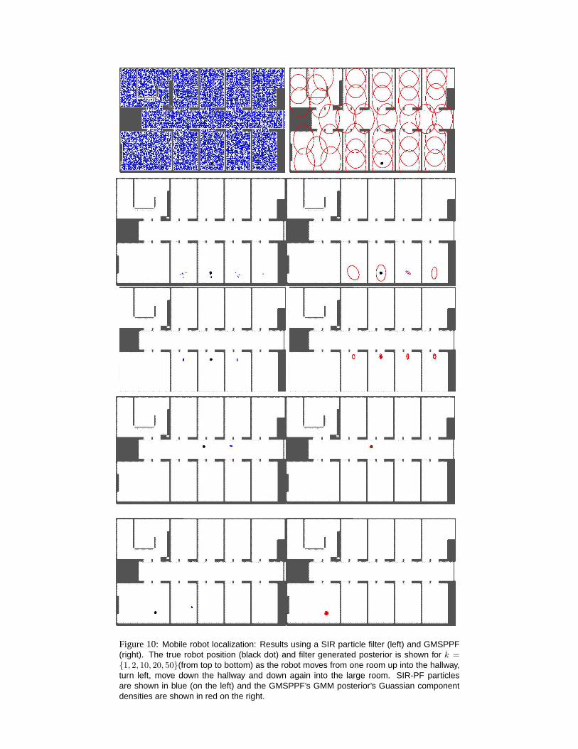
Figure 10 gives a graphical comparison of the localization results using a SIR particle fil-ter (SIR-PF) on the left and the GMSPPF on the right. The observation model used inthis example is based on a laser-range finder that measures distances to the closest wallsin a π/2 radian fan centered around the robots current heading. Due to the high accuracyof such a sensor, the measurement noise variance was set to a low value (σ = 10cm).The SIR-PF uses 20,000 particles (shown in blue) to represent the posterior and uses thestandard transition prior (movement model of the robot) as proposal distribution. Resid-ual resampling is used. The initial particle set was uniformly distributed in the free-spaceof the map. The GMSPPF uses 500 samples per Gaussian component, the number ofwhich are determined automatically using an x-means initialized EM clustering stage.The initial number of Gaussian components (shown in red) in the posterior was set to42, uniformly distributed across the free-space of the map. The SIR-PF quickly suffersfrom severe particle depletion even though 20000 particles are used to represent the pos-terior. At k = 10 (third plot from the top on the left) the SIR-PF has already lost trackof the true position of the robot. The GMSPPF in contrast accurately represent all pos-sible robot location hypotheses through multiple Gaussian components in its GMM pos-terior. As the ambiguity and uncertainty of the robots location is reduced, the numberof modes in the posterior decreases as well as the number of Gaussian component den-sities needed to model it. The GMSPPF accurately tracks the true position of the robotfor the whole movement trajectory. The superior performance of the GMSPPF over thatof the SIR-PF is clearly evident. Sample video files of the localization performance ofboth filters can be downloaded at:http://varsha.ece.ogi.edu/files/sirpf_mrl.mpg (SIR-PF)andhttp://varsha.ece.ogi.edu/files/gmsppf_mrl.mpg (GMSPPF).

7 Conclusions

Over the last 20 years the extended Kalman filter has become a standard technique withinthe field of probabilistic inference, used in numerous diverse estimation algorithms andrelated applications. One of the reasons for its wide spread use has been the clear under-standing of the underlying theory of the EKF and how that relates to different aspects of theinference problem. This insight has been enhanced by unifying studies towards the rela-

Figure 10:Mobile robot localization: Results using a SIR particle filter (left) and GMSPPF(right). The true robot position (black dot) and filter generated posterior is shown for k ={1, 2, 10, 20, 50}(from top to bottom) as the robot moves from one room up into the hallway,turn left, move down the hallway and down again into the large room. SIR-PF particlesare shown in blue (on the left) and the GMSPPF’s GMM posterior’s Guassian componentdensities are shown in red on the right.

tionship between the EKF and other related algorithms [36], allowing for the improvementof numerous existing algorithms and the development of new ones.

Recently, the unscented Kalman filter (UKF) and the central difference Kalman filter(CDKF) have been introduced as viable and more accurate alternatives to the EKF withinthe framework of state estimation. Like most new algorithms, these methods were notwidely known or understood and their application has been limited. We have attemptedto unify these differently motivated and derived algorithms under a common family calledsigma-point Kalman filters, and extended their use to other areas of probabilistic inference,such as parameter and dual estimation as well as sequential Monte Carlo methods. In doingso we have also extended the theoretical understanding of SPKF based techniques and de-veloped new novel algorithmic structures based on the SPKF. The SPKF and its derivativesare clearly set to become an invaluable standard tool within the “machine learning toolkit”.

References

[1] D. L. Alspach and H. W. Sorenson. Nonlinear Bayesian Estimation using GaussianSum Approximation.IEEE Transactions on Automatic Control, 17(4):439–448, 1972.

[2] B. Anderson and J. Moore.Optimal Filtering. Prentice-Hall, 1979.

[3] J. R. Cloutier, C. N. D’Souza, and C. P. Mracek. Nonlinear regulation and nonlinearH-infinity control via the state-dependent Riccati equation technique: Part1, Theory.In Proceedings of the International Conference on Nonlinear Problems in Aviationand Aerospace, Daytona Beach, FL, May 1996.

[4] I. J. Cox and G. T. Wilfong, editors.Autonomous Robot Vehicles. Springer Verlag,1990.

[5] J. F. G. de Freitas.Bayesian Methods for Neural Networks. PhD thesis, CambridgeUniversity Engineering Department, 1999.

[6] A. Doucet. On Sequential Simulation-Based Methods for Bayesian Filtering. Tech-nical Report CUED/F-INFENG/TR 310, Department of Engineering, University ofCambridge, 1998.

[7] A. Doucet, N. de Freitas, and N. Gordon.Sequential Monte-Carlo Methods in Prac-tice. Springer-Verlag, April 2001.

[8] D. Fox. KLD-Sampling: Adaptive Particle Filters. InAdvances in Neural InformationProcessing Systems 14, 2001.

[9] D. Fox, S. Thrun, F. Dellaert, and W. Burgard.Sequential Monte Carlo Methods inPractice., chapter Particle filters for mobile robot localization. Springer Verlag, 2000.

[10] A. Gelb, editor.Applied Optimal Estimation. MIT Press, 1974.

[11] Z. Ghahramani and M. Beal. Variational Inference for Bayesian Mixture of FactorAnalysers. InAdvances in Neural Information Processing Systems 12, 1999.

[12] S. Haykin, editor.Kalman Filtering and Neural Networks. Wiley, 2001.

[13] M Isard and A Blake. Contour tracking by stochastic propagation of conditionaldensity. InEuropean Conference on Computer Vision, pages 343–356, Cambridge,UK, 1996.

[14] Kazufumi Ito and Kaiqi Xiong. Gaussian Filters for Nonlinear Filtering Problems.IEEE Transactions on Automatic Control, 45(5):910–927, may 2000.

[15] A. Jazwinsky. Stochastic Processes and Filtering Theory. Academic Press, NewYork., 1970.

[16] S. Julier, J. Uhlmann, and H. Durrant-Whyte. A new approach for filtering nonlinearsystems. InProceedings of the American Control Conference, pages 1628–1632,1995.

[17] S. J. Julier. A Skewed Approach to Filtering. InSPIE Conference on Signal and DataProcessing of Small Targets, volume 3373, pages 271–282, Orlando, Florida, April1998. SPIE.

[18] S. J. Julier and J. K. Uhlmann. A General Method for Approximating NonlinearTransformations of Probability Distributions. Technical report, RRG, Dept. of En-gineering Science, University of Oxford, Nov 1996. http://www.robots.ox.ac.uk/siju/work/publications/letter_size/Unscented.zip.

[19] S. J. Julier and J. K. Uhlmann. A New Extension of the Kalman Filter to NonlinearSystems. InProc. of AeroSense: The 11th Int. Symp. on Aerospace/Defence Sensing,Simulation and Controls., 1997.

[20] R. E. Kalman. A new approach to linear filtering and prediction problems.Trans.ASME Journal ofBasic Engineering, pages 35–45, 1960.

[21] A. Lapedes and R. Farber. Nonlinear Signal Processing using Neural Networks: Pre-diction and System modelling. Technical Report LAUR872662, Los Alamos NationalLaboratory, 1987.

[22] T. Lefebvre, H. Bruyninckx, and J. De Schutter. Comment on ’A New Method forthe Nonlinear Transformation of Means and Covariances in Filters and Estimators’.IEEE Transactions on Automatic Control, 47(8), Aug 2002.

[23] Frank L. Lewis.Optimal Estimation. John Wiley & Sons, Inc., New York, 1986.

[24] J. Liu and R. Chen. Sequential Monte Carlo Methods for Dynamic Systems.Journalof the American Statistical Association, 93:1032–1044, 1998.

[25] M. Mackey and L. Glass. Oscillation and chaos in a physiological control system.Science, 197(287), 1977.

[26] C. J. Masreliez. Approximate Non-Gaussian Filtering with Linear State and Observa-tion Relations.IEEE Transactions on Automatic Control, AC-20:107–110, Feb 1975.

[27] G.J. McLachlan and T. Krishnan.The EM Algorithm and Extensions. Wiley, 1997.

[28] Andrew Moore. Very fast em-based mixture model clustering using multiresolutionkd-trees. In M. Kearns and D. Cohn, editors,Advances in Neural Information Pro-cessing Systems, pages 543–549, 340 Pine Street, 6th Fl., San Francisco, CA 94104,April 1999. Morgan Kaufman.

[29] Alex T. Nelson. Nonlinear Estimation and Modeling of Noisy Time-Series by DualKalman Filtering Methods. PhD thesis, Oregon Graduate Institute, 2000.

[30] M. Nørgaard, N. Poulsen, and O. Ravn. Advances in Derivative-Free State Estimationfor Nonlinear Systems. Technical Report IMM-REP-1998-15, Dept. of MathematicalModelling, Technical University of Denmark, 28 Lyngby, Denmark, April 2000.

[31] M. Norgaard, N. Poulsen, and O. Ravn. New Developments in State Estimation forNonlinear Systems.Automatica, 36, 2000.

[32] Dan Pelleg and Andrew Moore. X-means: Extending k-means with efficient estima-tion of the number of clusters. InProceedings of the Seventeenth International Con-ference on Machine Learning, pages 727–734, San Francisco, 2000. Morgan Kauf-mann.

[33] A. Pole, M. West, and P. J. Harrison. Non-normal and non-linear dynamic Bayesianmodelling. In J. C. Spall, editor,Bayesian Analysis of Time Series and DynamicModels. Marcel Dekker, New York, 1988.

[34] W. H. Press, S. A. Teukolsky, W. T. Vetterling, and B. P. Flannery.Numerical Recipesin C : The Art of Scientific Computing. Cambridge University Press, 2 edition, 1992.

[35] Yong Rui and Yunqiang Chen. Better Proposal Distributions: Object Tracking UsingUnscented Particle Filter. InProc. of IEEE CVPR, volume II, pages 786–793, Kauai,Hawaii, Dec 2001.

[36] A. H. Sayed and T. Kailath. A State-Space Approach to Adaptive RLS Filtering.IEEE Sig. Proc. Mag., July 1994.

[37] S. Singhal and L. Wu. Training multilayer perceptrons with the extended Kalmanfilter. In Advances in Neural Information Processing Systems 1, pages 133–140, SanMateo, CA, 1989. Morgan Kauffman.

[38] R. van der Merwe, N. de Freitas, A. Doucet, and E. Wan. The Unscented ParticleFilter. In Advances in Neural Information Processing Systems 13, Nov 2001.

[39] R. van der Merwe and E. Wan. Efficient Derivative-Free Kalman Filters for OnlineLearning. InProc. of ESANN, Bruges, April 2001.

[40] R. van der Merwe and E. Wan. The square-root unscented kalman filter for state andparameter-estimation. InProceedings of the International Conference on Acoustics,Speech, and Signal Processing (ICASSP), Salt Lake City, Utah, May 2001.

[41] R. van der Merwe and E. A. Wan. Gaussian Mixture Sigma-Point Particle Filters forSequential Probabilistic Inference in Dynamic State-Space Models. InProceedings ofthe International Conference on Acoustics, Speech, and Signal Processing (ICASSP),Hong Kong, April 2003. IEEE.

[42] Rudolph van der Merwe, Nando de Freitas, Arnaud Doucet, and Eric Wan. Theunscented particle filter. Technical Report CUED/F-INFENG/TR 380, CambridgeUniversity Engineering Department, August 2000.

[43] E. Wan, R. van der Merwe, and A. T. Nelson. Dual Estimation and the UnscentedTransformation. InNeural Information Processing Systems 12, pages 666–672. MITPress, 2000.

[44] E. A. Wan and R. van der Merwe. The Unscented Kalman Filter for Nonlinear Estima-tion. In Proc. of IEEE Symposium 2000 (AS-SPCC), Lake Louise, Alberta, Canada,October 2000.

[45] E. A. Wan and R. van der Merwe.Kalman Filtering and Neural Networks, Ed. SimonHaykin., chapter 7 - The Unscented Kalman Filter. Wiley, 2001.