19
B.Hargreaves - RAD 229 Signal Calculations • Bloch Equations and Matrix Calculations • Extended Phase Graphs • Examples (both) 113
| Date post: | 20-May-2018 |
| Category: |
Documents |
| Upload: | nguyenxuyen |
| View: | 217 times |
| Download: | 1 times |

B.Hargreaves - RAD 229
Signal Calculations
• Bloch Equations and Matrix Calculations
• Extended Phase Graphs
• Examples (both)
113

B.Hargreaves - RAD 229
Bloch Equation Matrix Simulations
• Basic Bloch Equation
• Bloch Equation with B1 / rotating frame
• Basic matrix simulations / Hard Pulse Approx.
• Many-spin simulations: Brute force
• Bloch Equation with Exchange
• Bloch-Torrey Equations (McNab?)
114

B.Hargreaves - RAD 229
Bloch Equation
• Basic Bloch Equation:
• In Matrix form with:
• Becomes:
115
dM
dt= M ⇥B � M
xy
T2+
M0 �Mz
T1
M =
2
4M
x
My
Mz
3
5
dM
dt=
2
4�1/T2 �B
z
��By
��Bz
�1/T2 �Bx
�By
��Bx
�1/T1
3
5M +
2
400
M0/T1
3
5

B.Hargreaves - RAD 229
Relaxation
• Over time period τ
116
E1 = e�⌧/T1
E2 = e�⌧/T2
M 0 =
2
4E2 0 00 E2 00 0 E1
3
5M +
2
400
M0(1� E1)
3
5

B.Hargreaves - RAD 229
RF Rotations• Over time period τ
117
M 0= R
x
M =
2
41 0 0
0 sin↵ cos↵0 cos↵ � sin↵
3
5M
M 0= RyM =
2
4� sin↵ 0 cos↵
0 1 0
cos↵ 0 sin↵
3
5M
↵ = �B1⌧

B.Hargreaves - RAD 229
RF Rotations (Arbitrary B1 phase)
118
R� =
2
4cos
2 ↵+ sin
2 ↵ cos� cos↵ sin↵(1� cos�) � sin↵ sin�cos↵ sin↵(1� cos�) sin
2 ↵+ cos
2 ↵ cos� cos↵ sin�sin� sin↵ � sin� cos↵ cos↵
3
5
� = tan�1(By
/Bx
)
• Note that Rφ is just Rz(φ)Rx(α) Rz(-φ)
B.Hargreaves - RAD 229
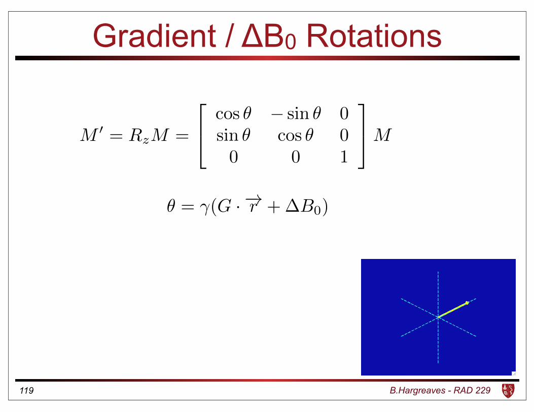
Gradient / ΔB0 Rotations
119
M 0= RzM =
2
4cos ✓ � sin ✓ 0
sin ✓ cos ✓ 0
0 0 1
3
5M
✓ = �(G ·�!r +�B0)
B.Hargreaves - RAD 229
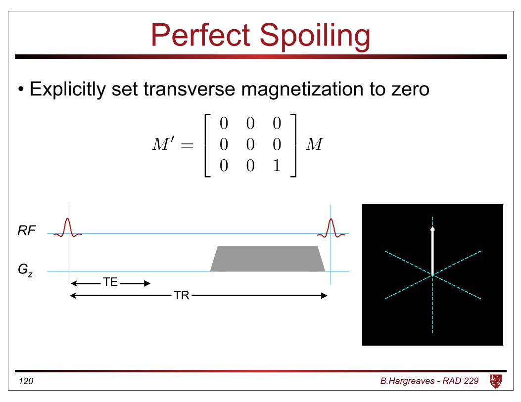
Perfect Spoiling
120
M 0 =
2
40 0 00 0 00 0 1
3
5M
• Explicitly set transverse magnetization to zero
RF
Gz
TRTE

B.Hargreaves - RAD 229
Example: Excitation/Recovery
M1 M2 M1 M2 M1 M2
α α α
1
Recall Prior Example!
B.Hargreaves - RAD 229
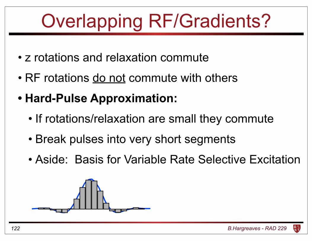
Overlapping RF/Gradients?
• z rotations and relaxation commute
• RF rotations do not commute with others
• Hard-Pulse Approximation:
• If rotations/relaxation are small they commute
• Break pulses into very short segments
• Aside: Basis for Variable Rate Selective Excitation
122
B.Hargreaves - RAD 229
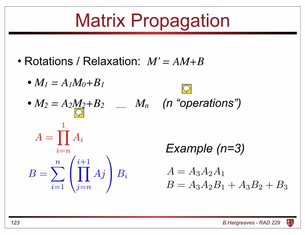
Matrix Propagation
• Rotations / Relaxation: M’ = AM+B
• M1 = A1M0+B1
• M2 = A2M2+B2 ..... Mn (n “operations”)
123
A =1Y
i=n
Ai
B = A3A2B1 +A3B2 +B3
A = A3A2A1B =nX
i=1
0
@i+1Y
j=n
Aj
1
ABi
Example (n=3)
B.Hargreaves - RAD 229
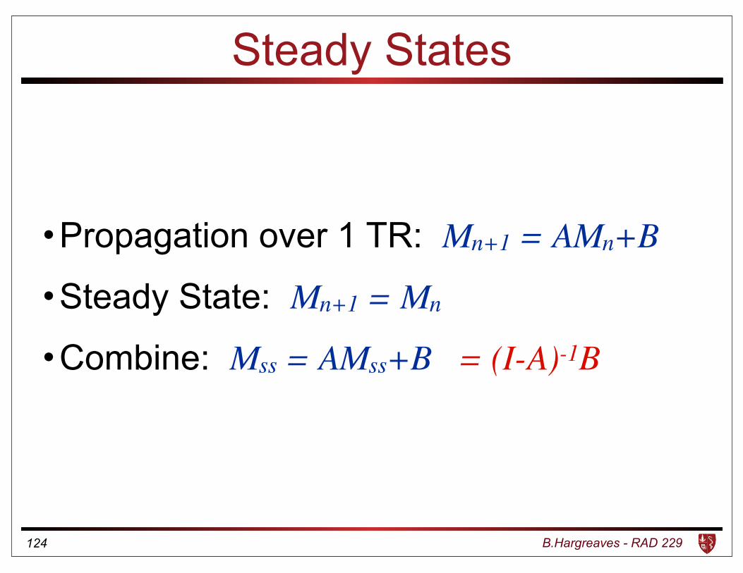
Steady States
•Propagation over 1 TR: Mn+1 = AMn+B
•Steady State: Mn+1 = Mn
•Combine: Mss = AMss+B = (I-A)-1B
124
B.Hargreaves - RAD 229
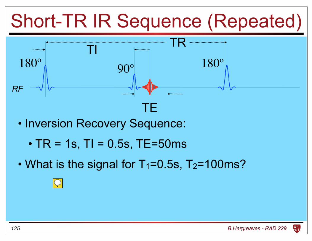
Short-TR IR Sequence (Repeated)
• Inversion Recovery Sequence:
• TR = 1s, TI = 0.5s, TE=50ms
• What is the signal for T1=0.5s, T2=100ms?
125
180º 180º
RF
TI
TE
TR
90º

B.Hargreaves - RAD 229
Example
• 90 Excitation pulse
• Time samples of 4µs
• 3 sync cycles
• 2ms duration
• Area of 5.9 µΤ*ms
• BW ~ 3 kHz
• 2.3 mT/m gradient (1kHz/cm)126
B.Hargreaves - RAD 229
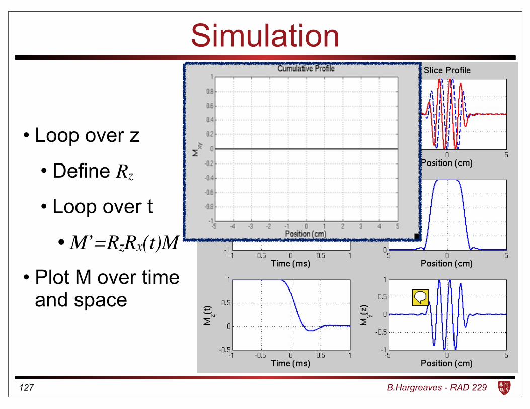
Simulation
• Loop over z
• Define Rz
• Loop over t
• M’=RzRx(t)M
• Plot M over time and space
127

B.Hargreaves - RAD 229
Example (Off-Resonance)
• 90 Excitation pulse
• BW ~ 3 kHz
• 2.3 mT/m gradient (1kHz/cm)
• 2kHz off-resonance??
128

B.Hargreaves - RAD 229
Excitation Recovery (Real Pulse)
• Simulate full pulse and position
• Perfect spoiling (“keep only Mz” matrix)
• Matrix propagation to calculate steady-state at each position
129
α=30
0 Mxy 0 Mxy
α=30 α=30
B.Hargreaves - RAD 229
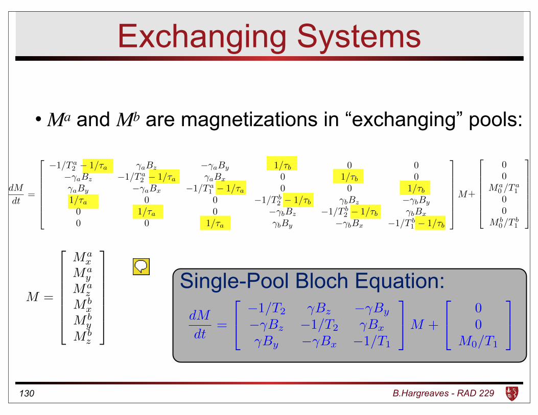
Exchanging Systems
• Ma and Mb are magnetizations in “exchanging” pools:
130
M =
2
6666664
Ma
x
Ma
y
Ma
z
M b
x
M b
y
M b
z
3
7777775 dM
dt=
2
4�1/T2 �B
z
��By
��Bz
�1/T2 �Bx
�By
��Bx
�1/T1
3
5M +
2
400
M0/T1
3
5
Single-Pool Bloch Equation:
dM
dt=
2
6666664
�1/T a
2 � 1/⌧a
�a
Bz
��a
By
1/⌧b
0 0��
a
Bz
�1/T a
2 � 1/⌧a
�a
Bx
0 1/⌧b
0�a
By
��a
Bx
�1/T a
1 � 1/⌧a
0 0 1/⌧b
1/⌧a
0 0 �1/T b
2 � 1/⌧b
�b
Bz
��b
By
0 1/⌧a
0 ��b
Bz
�1/T b
2 � 1/⌧b
�b
Bx
0 0 1/⌧a
�b
By
��b
Bx
�1/T b
1 � 1/⌧b
3
7777775M+
2
6666664
00
Ma0 /T
a1
00
M b0/T
b1
3
7777775

B.Hargreaves - RAD 229
Summary
• Bloch equation: Rotations and Relaxation
• Consider M as a 3x1 vector
• Rotations ~ Simple multiplier
• Relaxation ~ M’ = AM+B
• Propagate Effects like “Operators”
• Brute force simulations by looping:
• Time, Position, Frequency, etc
131


