SIGNAL PROCESSING FOR SENSOR BASED NAVIGATION …619179/FULLTEXT01.pdf · Buket Sonbas SIGNAL...

Buket Sonbas SIGNAL PROCESSING FOR SENSOR BASED NAVIGATION OF MOBILE ROBOTS

i

FACULTY OF ENGINEERING AND SUSTAINABLE DEVELOPMENT

SIGNAL PROCESSING FOR SENSOR BASED

NAVIGATION OF MOBILE ROBOTS

MSc Thesis

Buket Sonbas

Gävle/SWEDEN


ii

HÖGSKOLAN I GÄVLE FACULTY OF ENGINEERING AND

SUSTAINABLE DEVELOPMENT

SIGNAL PROCESSING FOR SENSOR BASED NAVIGATION

OF MOBILE ROBOTS

Buket Sonbas

September 2012

Master’s Thesis in Electronics

This thesis work has been submitted to Högskolan I Gävle Electronics/Telecommunications department in order to fulfill the requirement

of completing 30 ECTS credit for the degree of MSc in Telecommunications

Gävle/SWEDEN

Master’s Program in Electronics/Telecommunications

Examiner: Dr. JENNY IVARSSON

Supervisor 1: Prof. GURVINDER S. VIRK

Supervisor 2: Dr. JOSẺ CHILO


iii

Preface

I would like to dedicate my thesis work to my supervisor Prof. Gurvinder S. Virk for giving me

opportunity to write my thesis in Högskolan I Gävle and for his endlessly patience, mental and

educational support in every step of the work. I also want to send my deepest thanks to my second

supervisor Dr. Josẻ Chilo for his caring help and suggestions to improve my work.

Besides I would like to thank from all my heart to my precious family; mom, dad and my lovely

beloved sister; without their faith in me, I would not step up in the stairs of life alone.

Juan … world needs you!

All my friends who have a pure heart thanks for everything.


iv

Abstract

A self-navigating, path following and obstacle avoiding mobile robot is difficult to realize especially

when its sensors are strongly effected by noise. This MSc thesis is aimed at investigating a realistic

scenario of an autonomous mobile robot simulated in the MatLab environment. The robot system is

able to follow a given reference path by utilizing its onboard sensors and decision making capabilities

to avoid collisions with arbitrarily placed obstacles along its path. A novel navigational algorithm

based on modifying the robot’s way-points using the run-time sensory data is developed and used to

go around obstacles and then rejoin the original travel path as needed. The thesis work explores the

impact of varying noise in the sensory data and ways of improving the navigational accuracy via

signal processing. The study is done in two major sections, the first focusing on the navigational

aspects of the mobile robot and the second exploring the sensory data analyses issues.

The robot considered has a triangular shape with two differentially driven wheels at the rear left and

rear right corners for skid steering control and one castor wheel in the front corner for balance

purposes. The sensing system of the mobile robot includes infrared range finders with viewing angles

of 180 degrees placed on the corners of the robot, which are able to detect obstacles all around the

robot allowing effective path planning to be carried out via the special-purpose developed navigational

algorithms. A reference path in an obstacle cluttered environment is assumed to be available for the

robot to follow while avoiding randomly placed obstacles as the two wheels are driven to navigate the

robot along the path using the robot kinematics. For making the navigation mobility of the robot as

realistic as possible, practical infrared sensors have been studied experimentally to determine their

noise characteristics to include in the simulation studies and the noise levels easily varied to simulate

low and high noise levels and assess their effects on the overall navigational precision. Signal

processing methods are used to show that improvements in the navigational performance can be

achieved when the noise levels are high.

Keywords: Mobile robot, Signal processing, skid steering and castor wheels, navigation via way

points, reference path following


v

Table of Contents

Preface iii

Abstract iv

1 INTRODUCTION 10

1.1 BACKGROUND 10

1.2 STATEMENT 10

1.2.1 MOBILE ROBOT NAVIGATION 10

1.2.1.1 MOBILE ROBOTICS 10

1.2.1.2 NAVIGATION – PATH FOLLOWING – OBSTACLE AVOIDANCE 11

1.2.2 SIGNAL PROCESSING 12

1.3 THESIS OUTLINE 13

2 THEORY 14

2.1 NAVIGATION 14

2.1.1 WHEELED MOBILE ROBOT KINEMATICS 15

2.1.2 PATH FOLLOWING 16

2.1.3 OBSTACLE AVOIDANCE 20

2.2 SIGNAL PROCESSING FOR SENSOR DATA ANALYSIS 21

2.2.1 SENSOR 21

2.2.2 SENSOR TESTING HARDWARE 22

2.2.3 SENSOR TESTING SOFTWARE 26

3 PROCESSING AND RESULTS 29

3.1 SIGNAL PROCESSING 29

3.1.1 Sensor Calibration 29

3.1.2 Sensor Measurement Setup 30

3.1.3 Time and Frequency Domain 33

3.1.4 Sensor Response Time: 35

3.1.5 Sensor Noise Analysis 38

3.1.5.1 Stationary Obstacle Noise 38

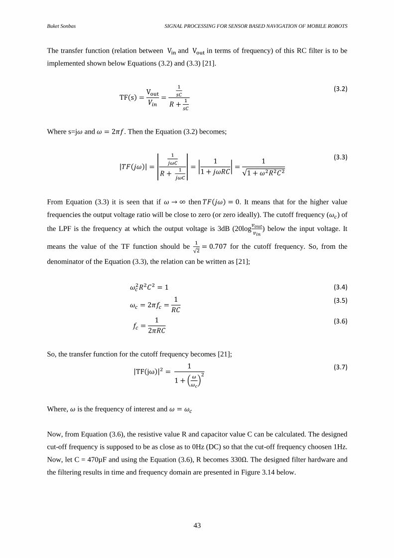
3.1.5.2 Software and Hardware Filtering (Design and Implementation) 42

3.2 MOBILE ROBOT 49


vi

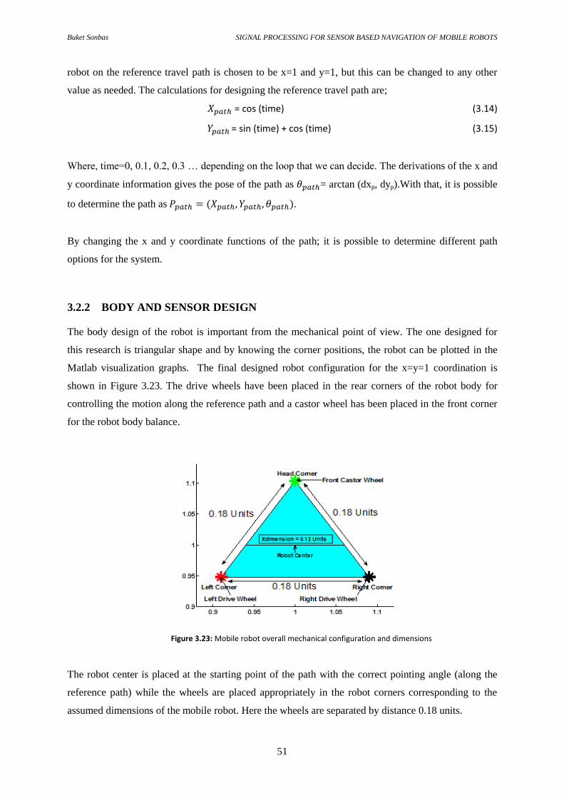
3.2.1 ROBOT LOCALIZATION IN THE 2D PLANE 50

3.2.2 BODY AND SENSOR DESIGN 51

3.2.3 PATH FOLLOWING 53

3.2.4 OBSTACLE AVOIDANCE AND DECISION MAKING 57

3.2.4.1 Obstacle Detection 58

3.2.4.2 Decision Making Algorithm 59

3.2.4.3 Simulation Results 64

3.2.5 EFFECTS OF NOISE IN SENSING 65

4 CONCLUSIONS 71

References 72

Appendix A 1


vii

List of Figures & Tables

Figures

Figure 2.1 Robot’s sensory-based perception and action behaviors in an unstructured environment 14

Figure 2.2 Mobile robot’s position and heading in a two dimensional coordinate system 17 Figure 2.3 Odometry systems to count wheel rotations via encoders on the wheels 18 Figure 2.4 Overview of the odometry for two wheeled systems 18

Figure 2.5 Analytical description of an ADC 23 Figure 2.6 Sampling example (sensor output vs. samples) 24 Figure 2.7 Resolution of a digital signal 25 Figure 2.8 Timing diagram of sensor measurement 27 Figure 2.9 Software diagram of DAQ 28 Figure 3.1 Sensor calibration set up and measurement results 30 Figure 3.2 Experimental set up for sensor measurement tests 31 Figure 3.3 Sensor without obstacle (a), sensor with a stationary obstacle in different distances (b) and sensor with

obstacle in different sampling frequencies (c) in time domain 32

Figure 3.4 Sensor reading in time and frequency domain 34 Figure 3.5 Data after removing DC level in time and frequency domain 34 Figure 3.6 Rotational moving obstacle hardware design 35 Figure 3.7 Rotational obstacle experiment results in (a) time, (b) frequency domains and the (c) velocity readings 36 Figure 3.8 Sensor response time analysis from enlarged view of Figure 3.7 (a) 37 Figure 3.9 Data after removing DC level in time and frequency domain 38 Figure 3.10 Schematic representation of by-pass capacitor addition 39 Figure 3.11 Probability density functions of sensor noise from Figure 3.9 40 Figure 3.12 Averaged standard deviation results of black and white boards in different distances from Table 3.2 41 Figure 3.13 RC LPF circuit diagram and ideal response graph 42 Figure 3.14 RC LPF design results in (a) time and (b) frequency domains and (c) hardware design 44 Figure 3.15 Circuit schematic of a forth-order butterworth LPF 45 Figure 3.16 Amplitude versus frequency response of a fourth-order Butterworth LPF 46 Figure 3.17 Lab setup figure for forth order Butterworth lpf 46 Figure 3.18 Data with and without 4th order Butterworth LPF in time (a) and frequency domain (b) 47 Figure 3.19 Probability density functions of reduced sensor noise from Figure 3.18 (σ = 0.0014) 47 Figure 3.20 Data filter comparison for software and hardware implementations in time (a) and frequency domain

(b) 48

Figure 3.21 Overview of the mobile robot navigation algorithm 49 Figure 3.22 Mobile robot visualization in the MatLab simulation environment 50 Figure 3.23 Mobile robot overall mechanical configuration and dimensions 51 Figure 3.24 Mobile robot sensor design 52 Figure 3.25 Mobile robot’s navigational results on different travel reference paths 55 Figure 3.26 Path following error in each step for Figure 3.25 (b) 56 Figure 3.27 Mobile robot obstacle detection 58 Figure 3.28 Navigational Algorithm 60 Figure 3.29 Mobile robot obstacle avoidance flow diagram 63 Figure 3.30 Mobile robot obstacle avoidance simulation results with different obstacle options (on a reference

path) 64

Figure 3.31 Navigation system implementation with the faulty data 65 Figure 3.32 Mobile robot’s sensory viewing cones with noise 66 Figure 3.33 Mobile robot navigation comparison with and without noisy sensor 66 Figure 3.34 Path following error in each step for Figure 3.25 (b) 67 Figure 3.35 Sum squared error comparison with different noise levels in noisy case without noise filtering 68 Figure 3.36 Sum squared error comparison with different noise levels in signal processing case with noise filtering 70


viii

Tables

Table 2.1 Different types of wheel 15

Table 3.1 Sensor data reading comparison 33

Table 3.2 Sensor response time data 37

Table 3.3 Sensor noise analysis with two different color stationary obstacles for different distances 41

Table 3.4 SSE comparison for different noise levels in noisy signal case 68

Table 3.5 SSE comparison for different noise levels in reduced noise signal case 69


ix

Abbreviations

FPX : Future Position X

MR : Mobile Robot

WMR : Wheeled MR

GPS : Global Positioning System

IPS : Indoor Positioning System

AMR : Autonomous MR

IR : Infrared

LED : Light-emitting diode

ADC : Analog to Digital Converter

DAQ : Data Acquisition

A/D : Analog/Digital

LSB : Least Square Bit

AOGND : Analog Output Ground

FFT : Fast Fourier Transform

DFT : Digital Fourier Transform

AI : Artificial Intelligence

AC : Alternartive Current

PDF : Probability Density Function

LPF : Low Pass Filter

BW : Butterworth

VDC : Voltage Direct Current

SSE : Sum Squared Error

http://sv.wikipedia.org/wiki/Massachusetts_Institute_of_Technology

http://en.wikipedia.org/wiki/Light-emitting_diode


10

1 INTRODUCTION

1.1 BACKGROUND

In November 2011, University of Gävle started a project in collaboration with Future Position X

(FPX) in Teknikparken Gävle entitled “Communicating mobile robots for automatic navigation and

control” aimed at designing and developing two mobile guide robots able to communicate and

navigate in realistic indoor environments. The two robots are felt to satisfy two specific and different

purposes but by communicating they are able to collaborate on their common goals. They have to

welcome guests and show visitors to the appropriate office after the initial greeting at the entrance of

FPX. The hosting robot is designed to be able to recognize which staff member is to be visited by

interacting with the guest using face recognition techniques after welcoming him/her and asking the

purpose of the visit. The other robot is the guide robot which is designed to receive the information

from the host robot via a specially designed communication system; this includes the destination

where to take the guest. In this way the guide robot should know its current location and the desired

location where it must navigate to. For reaching the desired location, the guide robot has to plan its

travel path (by using a map of the building) but in doing so it must avoid stationary or non-stationary

obstacles in its way. This thesis continues the development of the navigational strategy of the mobile

robot within a simulation environment. The research considers a typical mobile robot situation to

investigate the key problems and develops a realistic solution that can work on an actual robot

platform. In order to avoid obstacle on the travel path, the mobile robot is equipped with infrared

sensors to detect obstacles in the way and avoid as the robot moves to perform it intended mission. A

novel way to update the way-points is developed and tested to work well with and without sensor

noise.

1.2 STATEMENT

1.2.1 MOBILE ROBOT NAVIGATION

1.2.1.1 MOBILE ROBOTICS

The robots being developed in engineering departments are steadily improving to realize practical

systems for various applications. These include domestic, military, industrial, and medical systems. As

an important branch of robotics, mobile robots are also growing and it is becoming popular for

researchers and hobbysists who are interested to solve the complex navigational problems which arise.


11

In the middle of the 20th century, Walter [1] designed two small mobile robots able to find a light

placed in a dark room by avoiding plates placed between the robot and the light. When the robots were

started, first they found each other and when the light is on, they ignore each other and move towards

the light. Walter’s designs have inspired robot researchers to develop solutions to improve the

navigation of mobile robots by using different types of sensors. This work is still continuing today

with researchers trying to improve the control algorithms in terms of the robustness and autonomous

navigational capabilities of mobile robots so that they are able to meet the demands of the new

emerging service robot markets.

The mobile robot products are different for indoor or outdoor purposes because the coordinate planes

that they use are different. For example, agriculture and harvesting robots or search and rescue robots

operate in three dimensional (3D) unstructured environments and hence use 3D coordinates frames of

reference because they are designed to go up and down as well as in the x and y directions in the

horizontal plane [2]. Different purposes contains a wide variety of robots operating in various

domains; these can include robots for cleaning and housekeeping, automatic refilling, construction,

edutainment, fire-fighting, food industry, which are used as guides and assistants in offices, humanoid

robots, robots for inspection, medical robots, rehabilitation robots, surveillance and exploration robots

which can be legged or wheeled robots, using two dimensional (2D) or one dimensional (1D) frames

of reference to operate along the ground [2].

A robotic systems application requires a multidisciplinary approach to address and solve the various

issues in designing and developing a suitable solution. For example Electrical Engineering is needed

for the system integration, sensors and communication knowledge for the situation awareness and

information exchange, Computer Science for coding the planning algorithms, sensory data analysis

and control decision making for the basic motion capabilities, Mechanical Engineering for the

vehicle’s mechanisms and Cognitive Science for analyzing a variety of methods such as biological

organisms to develop smart and intelligent operational strategies [3].

This thesis work uses a 2D operational environment, Computer - Electronic – Mechanical Engineering

knowledge to complete the navigation task with appropriate processing of the sensory data.

1.2.1.2 NAVIGATION – PATH FOLLOWING – OBSTACLE AVOIDANCE

The main issues to be addressed for designing autonomous navigational strategies for mobile robots

are how they will estimate their pose within their environments using the installed sensors. The pose

includes the robot’s location (position within its environment) and its heading (the direction it is

facing). A wheeled mobile robot (WMR) is able to control its movement by controlling its drive


12

motors via a microcontroller and specialized software program embedded within it. A simple

odometry based localization method has been used in this thesis to localize the robot as it moves along

the reference path with a known starting pose.

Navigation in terms of mobile robots is aimed at reaching some desired point by avoiding collisions

with obstacles in the way. Two general kinds of navigation methods can be mentioned here, namely

global and local navigation. Almost all car users are familiar with GPS as a global positioning system

that takes satellite information which can map any place on the Earth and can be then used for global

navigation purposes. For indoor mobile robots, the GPS system does not work since it cannot receive

the data from the satellites because of the building causing an obstruction to block the signals. Other

systems are needed to provide the indoor localization information; such systems can be any kind of

vision-based or other distance ranging systems. These systems are called IPS (indoor positioning

systems). Indoor WMRs therefore require information of the robot’s environment so that the robot is

able to operate by navigating itself along a known map to perform an intended task such as follow a

given path trajectory within the map.

In this thesis a wheeled mobile robot is required to follow a reference travel path to reach a desired

location. In that sense, the geometry and kinematic constraints have to be studied and implemented to

navigate the robot to perform it’s intend task. In performing the path planning, the robot has a

reference path (within a map of its environment) and a goal that it has to reach on this reference path.

The robot is started at an arbitrary point on the reference path and it possesses the capability to update

its pose according to the trajectory it has to follow by points from where it is currently to the next

points along the travel path. These points are called way points and they need to be modified in real-

time as obstacles are encountered along the given travel path. The basic problem of this thesis is that

how the robot addresses the problems of updating the way-points to avoid obstacles and then rejoin the

original path when the obstacle has been avoided.

1.2.2 SIGNAL PROCESSING

While a wheeled robot follows the travel path to reach its target, it is clear that it can meet obstacles

such as humans, furniture, pets, etc. that are in its way. To avoid crashing into these obstacles, the

robot must have some suitable sensory and obstacle avoidance control systems to allow the

navigational strategy to be modified as needed. Infrared sensors are used to provide the environmental

data to the robot so that it is able to modify its motion properly. It is important to choose the correct

sensors for the required application and to study the full capabilities of the sensors and their behaviors

in terms of limitations so that fully informed decisions can be made under all situations. To understand

the infrared sensor behaviors, full range tests under static and dynamic situations are carried out


13

followed by detailed data analysis of the signals captured. These studies require work focusing on the

hardware and software aspects of the work that needs to be carried out.

The chosen sensor in this research is the Sharp IR range Finder sensor and its behavior has been

investigated from practical considerations to determine its noise characteristics and the results

implemented in the simulation studies to make the work as realistic as possible.

1.3 THESIS OUTLINE

This section gives a review of the thesis work and the key areas introduced. The overall work is

partitioned into the following sections:

A chapter on Theory which reviews the relevant theoretical aspects of navigating mobile robots

methods to determine which method will be suitable for the path following problem considered in this

thesis. The wheeled configuration of the mobile robot and its kinematics are also reviewed to derive

the path following controller strategy. The signal processing theory needed to handle the noisy signals

present in the infrared range sensor measurements is also presented to make the simulations as close to

real-world situations as possible.

A chapter on Process and results presents the method used to update the way points as the travel

reference path is tracked to ensure that the robot maintains collision-free navigation with and without

noise present in the sensory data. The mobile robot is simulated in the MatLab environment and

shown to follow the given travel reference path while avoiding the obstacles in its way.

The chapter presenting the main results is included where analyses of the main processes of the

research carried out is presented; this includes the reasons for the working methodology of the

navigational algorithm to update the way points in the obstacle free case, when an obstacle is

encountered, how the obstacle is avoided and how the robot returns to the original travel path when the

obstacle has been passed.

A Conclusion chapter summarizes the main findings of the research and suggests some work for the

future to further improve the navigational algorithm.


14

2 THEORY

This chapter presents the basic theory on the navigation, path planning, and obstacle avoidance used in

this research for the mobile robot considered. Some of the main path tracking methods presented to

give a good perspective for the navigation problem considered in the thesis using infrared range

sensors to detect obstacles around the travelling robot. A wheeled mobile robot is investigated and

simulated to study path tracking and obstacle avoidance tasks using methods from the area of mobile

robot navigation together with the signal processing needed when range sensory information becomes

corrupted with various levels of noise.

2.1 NAVIGATION

In Section 1.2.1.2 two kinds of navigation methods are mentioned, namely; indoor positioning systems

for navigation inside buildings and the global positioning system for general outdoor navigation. The

application considered in the thesis is an indoor guide robot having the ability to navigate

autonomously to some desired location in unstructured environments by following a reference travel

path using WMR kinematics and assuming the starting position is known.

By using multi-sensory data, it is possible to combine the overall data but then reduce the total

environmental information to get the necessary information needed for the navigation planning. For

example, when the environment needs to be scanned, the most important data is to determine the

leading edges of the nearest obstacles; it is these edges which must be avoided by the mobile robot if

collisions are to be avoided. So, rather than taking all the objects which could be monitored in the

operational environment, only the key features needed in the navigation have to be identified and used

in the decision making.

The overall process model used in sensor based navigation of mobile robots can be seen in Figure 2.1;

Figure 2.1: Robot’s sensory-based perception and action behaviors in an unstructured environment

ENVIRONMENT

Reaction Reaction

Interpretation

Signal

Interpretation

Sense


15

The sensors need to be matched to the operational environment, so that the obstacles can be detected

reliably and a robust navigational solution determined. In practice, measurements obtained by sensors

comprise noise (to varying degrees of level) and this can seriously affect the navigational performance

when it becomes excessive and so steps need to be adopt to reduce the effects of noise. This normally

involves the use of specially designed signal processing algorithms to reduce the effects of errors in

the measurements to allow more precise reaction interpretations in response to the sensed

environmental situations.

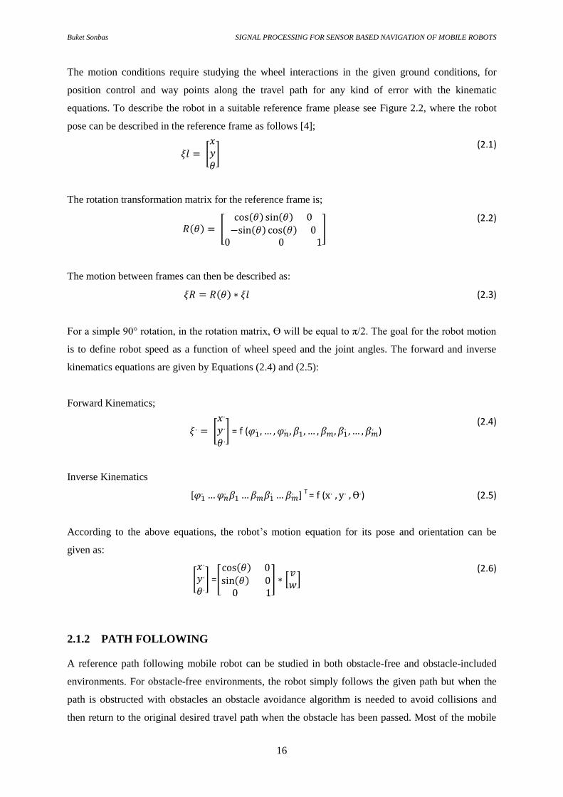
2.1.1 WHEELED MOBILE ROBOT KINEMATICS

Kinematics is the mathematical expression for describing the configuration of the mobile robot and

hence how the differentially driven wheels are controlled to make the robot travel in the manner

needed. In this section, the wheeled robots will be considered with respect to requirements of the work

to be carried out, although kinematic rules can be applied also for a wide variety of legged, armed and

flying robots. For motion control, wheeled robots use kinematic equations for the mathematical

modeling without considering the forces and dynamics for full modeling and motion control. For the

stability of a robot base, the wheel system should be well organized. A minimum of three wheels are

generally used to ensure good balance for a robot. However, the choice of wheels must be done for

ensuring that intend tasks can be carried out well when designing the robot.

Wheels are reviewed here and brief information is presented on standard wheels, castor wheels,

omnidirectional wheels, and spherical wheels [4]. Table 2.1 shows these types of wheels with their

main specifications;

Table 2.1 Different types of wheel [4]

Wheel type Specifications Figure

Standard Wheel Two degrees of freedom

Rotation around motorized axle and

contact point

Castor Wheel Three degrees of freedom

Rotation around wheel axle, contact

point and castor axle

Omnidirectional

wheel

Three degrees of freedom

Rotation around motorized wheel axles,

rollers, contact point

Spherical Wheel Suspension not technically solved


16

The motion conditions require studying the wheel interactions in the given ground conditions, for

position control and way points along the travel path for any kind of error with the kinematic

equations. To describe the robot in a suitable reference frame please see Figure 2.2, where the robot

pose can be described in the reference frame as follows [4];

[ ]

(2.1)

The rotation transformation matrix for the reference frame is;

( ) [ ( ) ( ) ( ) ( )

] (2.2)

The motion between frames can then be described as:

( ) (2.3)

For a simple 90° rotation, in the rotation matrix, Ө will be equal to π/2. The goal for the robot motion

is to define robot speed as a function of wheel speed and the joint angles. The forward and inverse

kinematics equations are given by Equations (2.4) and (2.5):

Forward Kinematics;

[

] = f (

)

(2.4)

Inverse Kinematics

[

] T = f ( ) (2.5)

According to the above equations, the robot’s motion equation for its pose and orientation can be

given as:

[

] =[

( ) ( )

] [ ]

(2.6)

2.1.2 PATH FOLLOWING

A reference path following mobile robot can be studied in both obstacle-free and obstacle-included

environments. For obstacle-free environments, the robot simply follows the given path but when the

path is obstructed with obstacles an obstacle avoidance algorithm is needed to avoid collisions and

then return to the original desired travel path when the obstacle has been passed. Most of the mobile


17

robots are designed in an environment with obstacles or other kinds of limitations so that the robot

should follow the normal kinematic constraints (Section 2.1.1) for good control and for achieving the

desired navigational performances.

For mapping of the environment, the floor plan can be provided and obstacle information can be

obtained using range sensors such as ultrasonic, laser range finders or depth vision cameras which

measure the open distance from the sensor to an obstacle in a specified direction. Scanning range

sensors are able to obtain multiple distances at different viewing angles which can be combined to

give the shape of an object in front of the sensor. If the sensors are placed at the front of the robot and

facing forward, the scanning sensor will determine the shape of the obstacle which the mobile robot is

facing. Laser ranging instruments are very precise distance measuring systems for measuring the

distances to obstacles around the robot.

Odometry:

Odometry is one of the most commonly used pose estimation methods which can be used for

differentially driven wheeled robots. The method works by using, for example, encoders on the wheels

or speed measurements to determine the wheel rotations over specific times to estimate the travel path

and hence determine the new position of the robot by updating the old known location. A differentially

driven wheeled robot can have two or more driven wheels which are controlled with a variety of

motors. The important things needed are the initial robot pose in the reference coordinate frame, the

wheel diameters, and the distance separating the driven wheels.

Assuming we have a triangular shaped mobile robot operating in a flat two dimensional coordinate

system (x, y directions); it has two differentially driven wheels on the rear corners to allow skid

steering to control the robot and a passive caster wheel at the front corner as shown in Figure 2.2. The

wheels can be chosen to be Ilon-wheels which are also called mecanum wheels or omni-wheels.

Figure 2.2: Mobile robot’s position and heading in a two dimensional coordinate system [5]


18

With odometry, the distance travelled information is obtained with encoders on the wheels to measure

the number of rotations of each wheel. The method assumes that there is no wheel slippage and the

wheel diameters are the same (different sized wheels can be used but this needs to be bourne in mind

in the calculations). Otherwise there are errors in the odometry and these can grow with time if not

reset regularly. Measuring the number of wheel rotation can be quite simple; for example, when the

encoders are located on the wheels, LEDs can be placed on the sides of the wheel and every time the

wheel rotates, as the encoder see the LEDs, the output signal will be received from the oscillator and

can be used to generate an appropriate digital signal, that is as a 0 or a 1, (1 represents that the encoder

has just seen the LED go by and 0 represents that the wheel is still completing its revolution). By

counting the digital “1” outputs, the number of wheel revolutions can be easily counted [6]. The

concept of this measurement system is illustrated in Figure 2.3;

Figure 2.3: Odometry systems to count wheel rotations via encoders on the wheels [6]

Using odometry to update the robot pose works as stated in Equations (2.7) – (2.14) via appropriate

mathematical expressions as described next (see Figure 2.4).

(a) Robot motion (b) Wheel angles

Figure 2.4: Overview of the odometry for two wheeled systems

Assuming that the robot’s starting pose is p and the travelled distances by the left and right wheels are

ΔSL and ΔSR respectively (shown as DSL and DSR in Figure 2.4), the new pose p’ can be calculated

as follows [6];


19

Left wheel motion is given by

(2.7)

Right wheel motion is given by

( ) (2.8)

Hence the overall robot motion is given by

(

)

(2.9)

And the change in the robot position is

( )

(2.10)

The robot’s change in it heading pointing angle is given by

(2.11)

The localization position change of the robot’s position in the X coordinate is given by

(

)

(2.12)

Similarly, the change in the Y coordinate position is given by

(

)

(2.13)

Hence the new robot pose is given by updating it from the previous as follows:

( ) [ ]

[

(

)

(

)

]

(2.14)

For a two wheeled mobile robot (and one passive castor wheel in the front), with the given Equation

(2.6) in Section 2.1.1 and Figure 2.2 in Section 2.1.2, the robot’s starting position can be located where

the path begins and the left and right wheel velocities can be calculated as follows [7];

(2.15)

(2.16)


20

Here vR and are the velocities of the right and the left wheels respectively, v is the tangential

velocity and w is the angular velocity of the robot, D is the distance between the two wheels. For a

reference path which can be described in both coordination as xp(t) and yp(t) in a time interval t, with

disregarding any kind of non-deterministic errors, the tangential and angular velocities and the

orientation of the robot in the reference path with time interval t, for forward and reverse directions are

presented next [7].

The tangential velocity is given by

( ) √ ( )

( ) (2.17)

The forward orientation is

( ) ( ( ) ( )) (2.18)

The reverse orientation is

( ) ( ( ) ( )) (2.19)

The angular velocity is given by;

( ) ( ) ( ) ( ) ( )

( )

( )

(2.20)

According to Equations (2.17) to (2.20), the derivatives of the curvature path variables are important.

It is clear that these equations can be applied only under the condition that the path is designed to be a

path which is at least twice differentiable.

2.1.3 OBSTACLE AVOIDANCE

As stated in Section 2.1, the environment of a mobile robot can contain obstacles so the navigation

method requires an obstacle avoidance capability. The principle of obstacle avoidance includes the

following aspects

Ability to sense obstacles

Ability to decide how to make corrective action to the travel path

Ability to act and take the action decided upon

The sensing, decision making and the action parts of the obstacle avoidance algorithm are discussed in

this section.


21

The aim of the MR can lead the robot designer to make suitable sensor choices so that the sensor

characteristics are satisfactory. When choosing the correct sensor, the highest priority is to ensure all

aspects are acceptable including the weight, size, kind of physical properties (both static and

dynamic). The interfacing of the sensor also needs to be considered so that the voltage ranges are

acceptable as well as other considerations such as the quality of the measurements, resolution of the

sensor, etc. For these reasons detailed sensor analysis should be carried out carefully by taking into

account the accuracy, sensitivity, power consumptions, etc.

For obstacle avoidance purposes, the sensor choice can be made with respect to the following range

sensors which are commonly used in mobile robot navigation applications: sonar sensors, laser range

finders, digital rgb stereo cameras, infrared sensors, etc. As already stated, due mainly to cost

considerations, infrared sensors have been adopted and tested for the research being presented.

After the sensing has been done, the algorithm for the decision making needs to be developed.

According to the sensing information, the decision making should be as clear and simple as possible

for fast reactions and it must cover all possible configurations that are likely to be encountered by the

mobile robot. Then of course the action part will be designed and implemented to perform the decision

that is made. For example, in a path following mobile robot, while there is no collision risk, the robot

can follow the desired travel path and when an obstacle is observed on the travel direction, a

modification is made to the travel path which goes around the object to avoid a collision, then the

obstacle contour is followed using a wall following algorithm until the object has been passed and the

original path is obstacle free again and then the actual travel trajectory path can rejoin the original

reference path. The obstacle avoidance algorithm should be done with respect to the locomotion goal

of the robot, the kinematics of the mobile robot, the precision of the range sensors, and ensuring that

the appropriate level of risk is taken to avoiding any actual or future possibilities of collisions.

2.2 SIGNAL PROCESSING FOR SENSOR DATA ANALYSIS

2.2.1 SENSOR

The infrared sensor choice is one of the most popular for today’s robotic experiences because of its

low price, easy usage, effective results, small convenient size, different ranging options, and short

response times. It also has low power consumption. Infrared sensors works using the triangulation

method which means that there are two lenses one which has the task to transmit the signal and the

other to receive the signal [8]. If the transmitted signal crosses an object (an obstacle) in front of it, the


22

signal will be received from the other lens with a point of reflection and this will create a triangular

path which will form an angle which helps to calculate the distance using the internal circuits of the

sensor. In that manner, the object’s positional distance in front of the sensor at a specific angle can be

determined. The beam width of the sensor is quite thin but finite, so there is a limit to the sizes which

can be detected; hence the sensor is more reliable in sensing larger objects. For sensing range while

designing an obstacle avoidance capability, it will be better to use a line scanning range sensor which

takes a distance reading at discrete points over a viewing angle. Laser range scanners having viewing

angles of 180-270° are now common with the possibility to select the number of readings that can be

obtained within the viewing angle. Some sensors have viewing angles which are much lower but in

principle it is possible to combine several of the sensors to be placed all around the sides of the robot

to ensure there are no blind points.

The sensor studied in this thesis work is the 2Y0A21 coded Sharp IR range sensor. The motivation for

this choice is the excellent features of this sensor; the most important characteristics are the following

[9]:

Measuring distance range = 10cm - 80cm;

Operating supply voltage = 4.5V to 5.5V;

Average supply current – typical = 30mA;

Response time = 39 ms;

LED pulse duration = 32 ms.

The main reason for choosing this particular sensor from the other family members is its distance

measuring capability which is felt to be ideal for obstacle avoidance. For this obstacle avoiding

purpose, a lower limit of the measuring distance cannot be less than about 10cm and the upper limit of

80cm is felt to be good. The response time is quite reasonable too, because when the robot meets the

obstacle, the response time will be enough for the making reaction of the robot in good time such as

stopping or changing the travel path by updating the way points to be travelled.

2.2.2 SENSOR TESTING HARDWARE

The sensor was calibrated to measure different distances using the a multi-meter and a graph plotted of

distance versus sensor voltage output; this is shown in Figure 3.1 (d) and the sensor’s calibration is

demonstrated against the manufacturer’s data sheet giving us confidence to use the sensor in other

experiments to construct the data acquisition hardware.


23

Commonly most sensors provide analogue signal outputs therefore analogue to digital conversion is

needed to interface them to digital computer systems. The first stage for this is data acquisition where

the analogue data is physically obtained from the analogue device through an analogue-to-digital

(ADC) interface which allows the computer to read the analogue signals at some selected sampling

rate.

In this system, the 2Y0A21 sensor has an analogue signal in the range 0 to about 3.5V output and an

ADC is needed to record the senor data for determining its characteristics. The data acquisition system

has been built with an ADC, an IR sensor, and a computer with suitable data acquisition software

accessible under MatLab.

An analogue signal is continuous whereas a digital signal has a discrete form. Computers operate

using binary bits. Mathematically speaking, an analogue/digital converter works as illustrated in

Figure 2.5 [10]:

A continuous signal can be represented as;

x (t) = A ( ) (2.21)

And a discrete signal can be represented as;

x (n) = A (

) (2.22)

So that the analogue to digital conversion schematic can be represented as;

x(t) x(n)

Figure 2.5: Analytical description of an ADC

Where t = continuous time

n = discrete time sampling instants

(t) = continuous input signal in the time domain

(n) = sampled output signal

Ф = phase

= frequency of the signal

= sampling frequency

To indicate a continuous analogue signal such as a sinusoidal signal in digitized form, there are two

things to consider; sampling at some sampling instants and quantization into a discrete number of

digitized levels [11], this means the continue analogue signal is digitized both in the horizontal time

direction by sampling and in the vertical direction by quantization.

A/D


24

Sampling implies taking a “sample” of the continuous signal at discretized time intervals. The time for

this discretization, t, is; t= ⁄ where the sampling rate or the sampling frequency is Fs. Equations

(2.21) and (2.22) shows that the ADC is converting the continuous signal in the time domain to a

sampled signal in the discrete form. The analogue output has a continuous time form that is being

converted by the ADC to its sampled form, in which the digital signal is only defined at the sampling

instants (n = 0, 1, 2, 3...).

To reconstruct the original continuous time signal from the discrete samples without significant error,

the highest frequency components of interest in the continuous signal to be sampled should be lower

than half of the sampling frequency; meaning that,

<

(2.23)

where; fmax = maximum frequency

fs = sampling frequency

This is known as the Nyquist sampling frequency [12]. For example, if the frequency of the analogue

signal is 1,000 Hz, then according to the Nyquist theorem, the sampling frequency should be more

than 2,000 Hz to ensure all the information is retained in the digitized signal. To have a more accurate

reading from the digitized signals, especially for control purposes (which depend on gain), it is

important to have much higher sampling rates. Suppose the signal is as represented in Figure 2.6;

Figure 2.6: Sampling example (sensor output vs. samples)

If the sampling frequency is not so frequent like the blue lines, the data between the sampling points

will be lost [13] and so having higher sampling rates will avoid losing any of the key and important

data where valuable information is to be found.

The ADC conversion can be done with a suitable data acquisition system and the device chosen in the

research work comprised the DAQPad-6020E from National Instruments. One of the important

considerations for choosing the device is its resolution which is 12 bits for performing the analogue to


25

digital conversion. The easiest way to understand the resolution is to look at a 1metre ruler which is

normally divided into centimeters; the 1cm “units” are the measurement units and these may turn out

to be too coarse especially if mm accuracy is needed. Hence, if much finer mm level accuracy is

needed the ruler must be divided into millimeters so that the measurement will be done more

accurately.

This number of discrete values over the full working range is the resolution. In digital systems the

digitally resolved analogue values are in binary form so that the resolution number is represented by 2

levels, 0 or 1 and binary numbers are written as 00 01 10 11 for a 2 bit word length which means that

there are 4 different levels which can be represented. This is obtained by using the formula and

similarly, if 3 bits word lengths are used, then the possible numbers are 000 001 010 011 100 101 110

111 which mean that there are 8 different levels which are given by using etc... For an 8 bit word

representation the resolution will allow binary numbers which means 256 levels. If the output of

the sensor is in volts, then the minimum change in voltage which can be presented will be equal to

(overall voltage range) / (number of discrete values) [14]. According to that, the more the resolution,

the closer the discrete signal will be to the original signal. In this thesis, the overall voltage is from 0V

to ≈5V and as the ADC resolution is 12 bits [14], then the minimum voltage change will be according

Equation (2.24);

Resolution = R =

≈ 1.2 mV (2.24)

This resolution is felt to be good enough for our application. From the previous discussion, it is

understood that the analogue signal is continuous and the digital signal is discrete. This leads the

following digital forms (in quantized form) if the analogue signal is as shown in Figure 2.7 (a-b);

(a) Digital and analogue version of signal in 3bit

resolution

(b) Enlarge view of the signal

Figure 2.7: Resolution of a digital signal

According to Figure 2.7 (a), every level of the signal in our case (Equation (2.24)) is changing with

1.2mV resolution in the numbers. Since the ADC device resolution is 12 bits, the difference in voltage


26

going from 000000000000 to 000000000001 will be 1.2mV. With this calculation, the error is

inevitable but small enough and manageable. Figure 2.7 (b) is the maximized illustration of one level

of Figure 2.7 (a). If the original value is in between two LSB (least significant bit), the system will

read the value as the nearest upper LSB but this will not be the exact value [15]. The original value is

in between + ( ⁄ )*LSB to - ( ⁄ )*LSB. So, it is important to consider this error in the calculations.

This error is called the quantization error and can be calculated by the Equation (2.25) below;

Quantization error =

* LSB (2.25)

The DAQPAD-6020E has a brief datasheet for connections and measurements. For setting up the

hardware, the connections have been made according to the device’s pin outs [14]. The interface of the

sensor is 3-wires comprising ground, power in and the output (see Appendix A). ACH1 is the

analogue input channel chosen where the sensor is connected, +5 V is the power in port and AOGND

is the analogue output ground from the board [14]. After connecting the sensor and the other inputs the

software aspects can be focused upon. There are many software choices but two of the choices are

readily available in the data acquisition system the first uses LabView and the second uses MatLab. In

this work MatLab 7.01 is chosen to allow more familiarity with it as it was used in the mobile robot

simulations.

2.2.3 SENSOR TESTING SOFTWARE

Here the ADC is used to convert the analogue sensor signals to digital format using 12 bit resolution.

The data acquisition toolbox of MatLab helps to get data from sensors through the ADC unit. With

MatLab, it is possible to decide the sample rate, plan the events, store and plot the data collected,

perform data analysis, etc.

The sensitivity of the measurements depends on the resolution and the amplitude of the sensor signals.

To resolve the issue of frequency, a decision on the highest frequency of importance and needing to be

measured needs to be made; this depends on the device’s bandwidth. In that case, the key point is the

sensor’s timing diagram. According to the datasheet, for the highest frequency of the device, the

timing diagram shown in Figure 2.8 is provided [9].


27

Figure 2.8: Timing diagram of sensor measurement

The time taken to take to repeat the measurements given in manufacturer’s datasheet is 38.3±9.6ms.

From this period, the lowest and the highest frequencies can be calculated as =1/t = 1/28.7ms ≈

35 Hz and =1/t = 1/47.9ms ≈ 21 Hz. As the LED pulse duration is around 32ms and the typical

response time is around 39ms, the reasonable highest frequency will be chosen 35Hz. To be able to

measure the response of the sensor, it is required to fulfill the Nyquist frequency theorem in order to

avoid loss of information. From the Nyquist frequency theorem, it is known that the minimum

sampling frequency should be more than 2F where F is the possible highest frequency of the original

signal. In implementation it is suggested that the sampling frequency should be at least 10 times of the

highest frequency of the signal. Choosing the sampling frequency at least 10 times of the original

signal frequency ensures the better resolution of the measurement from the ADC (DAQ-Pad 6020E)

[16].

The sensor signals depend on their polarities as there are two kinds of polarity, namely unipolar and

bipolar. Unipolar signals contain the positive values (starting from zero) and bipolar signals contain

both positive and negative values [17]. The Infrared 2Y0A21 sensor produces unipolar signals [9]. For

the channel configuration this need to be set to single ended.

The reason that signal processing knowledge is highly important is because of the ever presence of

signal noise and the need for noise reduction in most real-world applications. Noise in the signal

normally means unwanted random additions [18]. In a sound or an image signal, noise can cause

distortion or changes to the information signal. There are many reasons for noise in signals but

actually noise exists in all the inner circuits of devices as thermal noise caused by random movement

of charges (internal noise). Sensor systems can easily be affected from environmental reasons as well

(external noise). The effect of noise can be reduced by appropriate filtering; both in hardware and via

software. We will focus on software filtering or as it is commonly referred to as signal processing.

The terminology of the data acquisition system used needs to be stated; in the DAQ Toolbox of

MatLab, the name of the device that will be used is “nidaq”. There are several steps to follow in

MatLab [19] as shown in Figure 2.9;


28

Figure 2.9: Software diagram of DAQ

By plotting the sensor data collected, the analysis can start. The sensor gives different voltage results

in measuring different distance ranges. In the time domain it is expected to see a plot of the signal

voltage vs. time. The plot will show how the signal is varying and when. Information that the time

domain provides is the time, periodicity and the amplitude. The duration depends on the trigger and

the sampling frequency. For plotting the signals in the frequency domain, the use of FFTs (Fast

Fourier Transforms) are required. The definition of FFT can be given from the Discrete Fourier

Transform (DFT) [13]. The mathematical expression of DFT can be described by the following

Equation (2.26);

= ∑

k=0,1,…, N-1 (2.26)

Where is the input data in time domain having length of and is the output data in frequency

domain having length of . To calculate DFT by this equation times of computations are needed.

With the FFT algorithm, the number of computation can be reduced from to by making

two equations from the even and odd numbers of such as;

∑

(

)

(

)∑

(

)

(2.27)

This way, the algorithm reduces the number of computations so that the computation will be faster.

The noise problem should be investigated by extracting the data from the sensor via ADC to ensure

good navigational algorithms under noisy and noise-free situations. The noise is a random addition to

the measurement of sensor’s signal. It exists in every measurement randomly with the desired signal.

For that reason, the measurements must be done several times to determine the statistical patterns of

the sensor’s signal.

Configuring the sample rate and duration to decide the resolution and duration of the signal

Adding the input type of the system ‘Single Ended’

Ranges; Sensor is unipolar so range is from 0 to 5V

Extracting the Data with ’get (data)’ command

Creating the analog input with ’AI’ command to access the DAQPAD device and adding hardware channels for “AI”


29

3 PROCESSING AND RESULTS

3.1 SIGNAL PROCESSING

A navigational algorithm should be observed under a simulated environment with a noise-free sensor

signal, a noisy sensor signal and a sensor signal after noise reduction. The main purpose of the signal

processing for sensor based navigation of mobile robot is to find out and reduce the influence of the

noise in the sensor signal and observation of the noise effect in navigational performance. This chapter

includes the comparison of the sensor signal results with and without signal processing. The steps for

the sensor signal analysis for the noise reduction are briefly described as follows;

1) Calibration of the sensor: the sensor should be tested with a basic system for its calibration.

The expected results from this sensor are voltage responses versus distance of the object. The

comparison can be made with the manufacturer’s datasheet.

2) Sensor measurements setup: the sensor readings need to be closely analyzed on a computer

via an ADC with an embedded program to see the readings of the sensor. For this purpose, a

reliable setup should be developed.

3) Sensor readings in time and frequency domains: the readings of the sensor in the computer

should be clarified in the time domain to see the sensor behavior. The frequency information

should be displayed to check the frequency response characteristics of the sensor.

4) Sensor noise: as it is predictable, all electronic devices includes a noise addition for different

reasons. The noise of the sensor should be studied to determine its characteristics and include

these in studying its effects on the mobile robot navigation strategy.

5) Measuring moving obstacles: this kind of test is necessary to understand the sensor’s dynamic

behavior with an obstacle moving at different speeds.

3.1.1 Sensor Calibration

Before starting the analysis of the infrared sensor, the user must be sure it is calibrated properly. With

a setup, using a power supply, a multi-meter and the chosen infrared sensor 2Y0A21, the output to

indicate the distance, an object is placed in front of the sensor. The datasheet for the sensor shows

what the voltage value is expected corresponding to the distance between an obstacle and the sensor.

An experimental system is designed and constructed to measure the change in voltage with the

distance (See Figure 3.1 below). The distance measurement outputs with the obstacle placed at

different distances from the sensor have been measured. The measurement results have been recorded

manually (from 10cm to 60cm in steps of 2cm). The results are shown in Figure 3.1.


30

(a) Calibration set up schematic (b) Calibration set up figure

(c) Calibration results with curve fitting (Distance

vs. Voltage)

(d) Calibration results comparison with the

manufacturer’s datasheet (Distance vs. Voltage) [9]

Figure 3.1: Sensor calibration set up and measurement results

The data can be fitted better with a polynomial of order 4 (y=a+bx+cx2+dx

3+ex

4) as shown in Figure

3.1 (c). The results are similar to the manufacturer’s datasheet as shown in Figure 3.1 (d) above.

3.1.2 Sensor Measurement Setup

For proper data acquisition of the measurement signals from the sensor, it is mandatory to design a

reliable setup which gives efficient results. Moreover, the obtained measurement data have to be

verified for moving and stationary obstacles to understand the behavior of the sensor.

10 20 30 40 50 600

0.5

1

1.5

2

2.5

Distance [cm]

Vo

ltag

e O

utp

ut

[Vo

lts]

Multimeter Results with Curve Fitting

Multimeter results

quadratic fitting

cubic fitting

4th degree fitting

10 20 30 40 50 600.5

1

1.5

2

2.5

Distance [cm]

Vo

ltag

e O

utp

ut

[Vo

lts]

Datasheet vs Multimeter Measurements

Manufacturer's Datasheet

Multimeter Measurements


31

The data acquisition has been done in different conditions including the following

Sensor without obstacle (no obstacle placed in the sensor range up till 80 cm).

Sensor with stationary obstacle (a white and a black board). Sensor noise characteristics can be

analyzed with this kind of experiment.

Sensor with rotational obstacle such as a propeller fan having 2 rectangular straight blades (See

Figure 3.2 (c)). The sensor response time can be analyzed with this kind of experiments.

Figure 3.2 illustrate the schematic diagram of the designed set up to acquire data from the sensor.

(a) Lab setup schematic (b) Lab setup figure

(c) Rotational moving obstacle

Figure 3.2: Experimental set up for sensor measurement tests

For the stationary obstacle, a white board and for the non-stationary obstacle, a rotating fan is used.

The experimental system is used to test the IR range sensor and the measured data displayed on the

computer by converting the signals using an ADC via MatLab. All those measurements are repeated

several times to compare the voltage outputs depending on the different distances with the datasheet


32

results. Figure 3.3 shows the time domain plots of the measured data, without obstacle results, with

different distanced (stationary) obstacles from the sensor, and the data with different sampling

frequency results.

(a) Sensor without obstacle (b) Sensor with obstacle ( obstacle- sensor distances at

10m, 20cm, 30cm, 40cm, 50cm, 60cm, 70cm, 80cm)

(c) Sensor readings in different sampling frequencies

Figure 3.3: Sensor without obstacle (a), sensor with a stationary obstacle in different distances (b) and sensor with obstacle

in different sampling frequencies (c) in time domain

The measurement in Figure 3.3 (a) has been done using the sampling frequency of 500 Hz and the

length of the signal is 2500 samples (5 seconds of data) as it has been discussed in Section 2.2.3. Data

with the different sampling frequencies also is plotted and presented for a comparison in the Figure 3.3

(c). The sensor reading without obstacle shows that the voltage level is very low since the sensor does

not detect any obstacle. Also the result shows that the signal is corrupted with noise. Figure 3.3 (b)

0 1 2 3 4 50

0.1

0.2

0.3

0.4

0.5

Time [Seconds]

Vo

ltag

e O

utp

ut

[Vo

lts]

Sensor Data Without Obstacle

0 1 2 3 4 50

0.5

1

1.5

2

2.5

3

Time [Seconds]V

olt

ag

e O

utp

ut

[Vo

lts]

Sensor readings in different distances

10 cm

20 cm

30 cm

40 cm

50 cm

60 cm

70 cm

80 cm

0 1 2 3 4 5 1

1.2

1.4

1.6

1.8

2

2.2

2.4

2.6

Time [Seconds]

Vo

ltag

e O

utp

ut

[Vo

lts]

Data with different sampling frequencies

500 Hz 600 Hz

1,500 Hz

3,000 Hz

10,000 Hz

800 Hz 200 Hz


33

shows that the signal voltage level is different in each distance level. Table 3.1 is given below to

compare the acquisition results in Figure 3.3 (b) with the manufacturer’s datasheet.

Table 3.1 Sensor data reading comparison [9]

Distance from sensor [cm] Datasheet Reading [V] ADC reading [V]

10 ≈ 2.32 ≈ 2.38

20 ≈ 1.30 ≈ 1.31

30 ≈ 0.94 ≈ 0.94

40 ≈ 0.75 ≈ 0.75

50 ≈ 0.62 ≈ 0.60

60 ≈ 0.52 ≈ 0.52

70 ≈ 0.45 ≈ 0.45

80 ≈ 0.41 ≈ 0.42

The Section 2.2.2, it’s been discussed that, Nyquist Frequency Theorem is one of the most important

criteria for deciding the sampling frequency. Moreover, for a better resolution of the acquired data

from ADC, the sampling frequency should be at least 10 times bigger than the highest frequency of the

sensor. The sensor’s highest frequency is calculated 35 Hz. In this case, the sampling frequency should

be above 350 Hz. The Figure 3.3 (c) shows the comparison for 200 Hz, 500 Hz, 600 Hz, 800 Hz, 1.5

KHz, 3 KHz, and 10 KHz. The results are plotted in different distances only for a better presentation

of the figure (200 Hz at 10cm, 500 Hz at 11cm, 600 Hz at 12cm, 800 Hz at 14cm, 1.5 KHz at 16cm, 3

KHz at 20cm, 10 KHz at 25cm). The data in 200Hz does not comply with the requirement of ADC

resolution; therefore, the data is still acquired but not as good resolute as in 500Hz. The rest of the

frequencies show that there is no change in sensor data but a better resolution on signal presentation.

Another rule for choosing the sampling frequency is that the limit for ADC should be considered. In

DAQ-Pad 6020E the maximum sampling frequency is 100 KHz [14] and cannot be exceeded.

3.1.3 Time and Frequency Domain

The presentation of a signal is important for the analysis. For example in Figure 3.3, it is possible to

visualize the signal time but it is not possible to have frequency information of the signal. Therefore,

frequency domain should be studied as well. As discussed in Section 2.2.3, a preferable method for a

frequency domain reading is the Fast Fourier Transform. The frequency domain signal is presented in

this section by using Signal Processing Toolbox of MatLab (See Figure 3.4 below).


34

(a) Data measured at 80 cm distance from sensor in

time domain

(b) Frequency domain of the data

Figure 3.4: Sensor reading in time and frequency domain

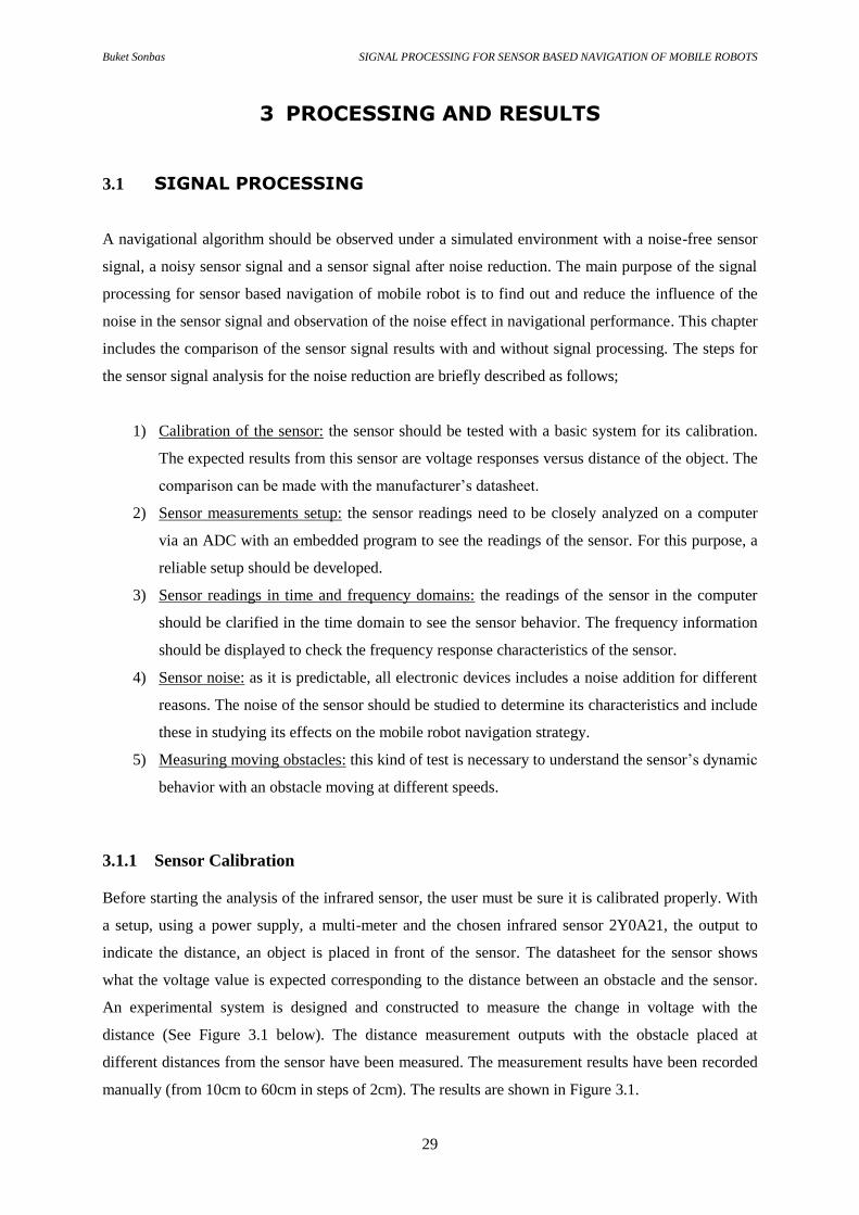
The Figure 3.4 shows the sensor reading with the obstacle at distance 80 cm. Data has been plotted for

1 second to show the sensor reading in a clear view. The sensor voltage output for this distance is

approximately 0.42V. The frequency domain representation shows relatively high amplitude (0.4364)

at 0Hz and the rest information. The desired output from the sensor is only a DC voltage and it has no

frequency (zero Hz). The rest information in the frequency domain is noise because there is no other

frequency information expected from the sensor.

The time domain representation clearly shows that the signal is corrupted with noise as discussed

before. In normal approach for studying the noise in experimental data requires removing DC signal.

In Figure 3.5, the signal is presented after removing DC level. When removing the DC level from the

signal, the frequency domain representation shows the noise clearer.

(a) Data after removing DC level in time domain (b) Data after removing DC level in frequency domain

Figure 3.5: Data after removing DC level in time and frequency domain

0 0.2 0.4 0.6 0.8 10.4

0.45

0.5

0.55

0.6

0.65

Time [Sec]

Vo

ltag

e [

V]

Data in time domain (obstacle at 80 cm)

0 50 100 150 200 2500

0.1

0.2

0.3

0.4

0.5

X: 0

Y: 0.4364

Frequency [Hz]

Am

plitu

de

Data in frequency domain

0 0.2 0.4 0.6 0.8 1-0.1

0

0.1

0.2

0.3

0.4

0.5

0.6

Time [Seconds]

Vo

ltag

e [

Vo

lts]

DATA IN TIME DOMAIN

0 50 100 150 200 2500

0.005

0.01

0.015

0.02DATA IN FREQUENCY DOMAIN

Frequency [Hz]

Am

plitu

de


35

3.1.4 Sensor Response Time:

As discussed in Section 3.1.2, the sensor response time analysis is done with a rotational fan that

creates an obstacle motion in which the sensor is sensing the obstacle and then not. This type of

motion has a frequency component since the motion is repeated several times in one second.

The rig shown in Figure 3.2 (c) is mainly designed in three parts; part one is the main fan system

running with a 6 VDC motor (see Figure 3.6 (a) below), part two is an encoder (see Figure 3.6 (b)

below) to measure the speed via a microcontroller (Arduino Uno), part three is the motor controller

system with a hardware (see Figure 3.6 (c-d) below) and a microcontroller (Arduino Mega ADK).

(a) Part one of the rig; the fan (b) Part two of the rig; the encoder

(c) Part three of the rig; the motor controller (d) Motor controller circuit diagram

Figure 3.6: Rotational moving obstacle hardware design

The main fan system is designed by using a 6VDC motor with a gear ratio of 1:3. The motor controller

system has a potentiometer (100k) to adjust the speed of the motor, a power transistor with a heat sink

(IRF 520 N MOSFET) which has designed for high-current loads, a power supply (6 V) to feed the

system, and a diode to protect the transistor from backfiring voltage which might be caused by two


36

reasons; when the motor shuts down or when the motor polarity is being switched. The motor is

controlled with help of the Arduino Mega ADK with a program embedded and the speed variation is

controlled with the potentiometer. The encoder also is connected to the fan mile. The speed reading

from the fan is acquired with Arduino software program while the encoder is connected to the Arduino

Uno Board and plotted in Matlab.

When the Fan runs, the sensor acquires the data from Matlab. Figure 3.7 presents an example of the

speed readings of the motor via encoder and the sensor readings in time and frequency domain for that

speed level.

(a) Rotational motion measurement in time domain (b) Rotational motion measurement in frequency

domain

(c) Rotational motion velocity readings from encoder

Figure 3.7: Rotational obstacle experiment results in (a) time, (b) frequency domains and the (c) velocity readings

The Figure 3.7 above represents the fan motion readings from the sensor when the distance between

fan wings and the sensor is 14 cm. The maximum reading in time domain is 1.8 Volt and the minimum

reading is around 0.2 Volt since the sensor is measuring once the fan blades and then no object

repeatedly. Frequency domain readings show that the motion frequency is 5.005Hz and this means that

the sensor reads the fan blades 5 times in a second. The speed readings from the encoder are taken

0 1 2 3 4 50

0.5

1

1.5

2

Time [Sec]

Vo

ltag

e [

V]

Rotational motion in time domain

0 50 100 150 200 2500

0.1

0.2

0.3

0.4

0.5

0.6

0.7

X: 5.005

Y: 0.2439

Frequency [Hz]

Am

plitu

de

Frequency domain

0 1 2 3 4 54

4.5

5

5.5

6

Time [Sec]

rps

Velocity of Fan Blades


37

with Arduino embedded coding and plotted in Matlab and the average velocity of the fan blades are 5

revolutions per second. This means that the fan blades are crossing the sensor line 5 times in one

second. As a conclusion of the fan velocity measurement, it can be verified that the measurements are

correct in Arduino programming since the frequency domain readings are complementing each other.

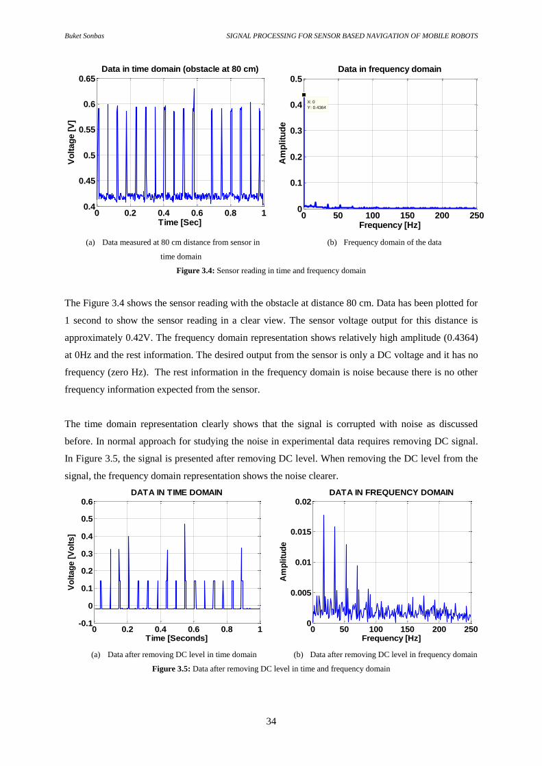
The sensors cannot change their output instantly regarding a change in the input. It is important to

have a sensor which responds almost instantly, therefore the response time analysis is important. For

example a navigation system based on sensor response, if the sensor does not response in a very short

time after its measurement, the navigating robot collision is unavoidable. The speed of the response

can be predicted in both time and frequency domains. In this experiment, a time domain method is

used to calculate the sensor response speed. To do that, the sensors time constant will be taken into

account. To determine the response time of the sensor, let’s have a closer look to the measurement in

time domain.

(a) Rising time of the sensor response (b) Decay time of the sensor response

Figure 3.8: Sensor response time analysis from enlarged view of Figure 3.7 (a)

In Figure 3.8, for the rising time and decay time voltage information versus time information is given

in the Table 3.2 below;

Table 3.2: Sensor response time data

Rising time information Decay time information

Voltage (V) Time (Sec) Voltage (V) Time (Sec)

0.31013 0.224 1.8144 0.262

0.29548 0.226 1.8193 0.264

0.30525 0.228 1.8168 0.266

1.8217 0.23 0.24664 0.268

1.8242 0.232 0.23932 0.27

1.8168 0.234 0.25153 0.272

0.21 0.215 0.22 0.225 0.23 0.235 0.240

0.5

1

1.5

2

Time [Sec]

Vo

ltag

e [

V]

Enlarged view of one pulse in time domain

0.25 0.255 0.26 0.265 0.27 0.275 0.280

0.5

1

1.5

2

Time [Sec]

Vo

ltag

e [

V]

Enlarged view of one pulse in time domain


38

Given array in Table 3.2 of the enlarged view in Figure 3.8, the red marked numbers are the decay and

rise times. The voltage reading shows that there is a big difference and the pairing time readings of the

rise and decay times are 0.002 seconds.

3.1.5 Sensor Noise Analysis

3.1.5.1 Stationary Obstacle Noise

Both the time domain signal and the frequency domain signal in Figure 3.4 demonstrate that the signal

is corrupted with noise. The spikes which have relatively high amplitude is not entirely conclusive

that from where they come from, but the possible cause could be the internal circuitry of the sensor

(quality of the sensor), leakage between the sensor ports or ripple voltages from the power supply

line. The spikes can be reduced simply with using a by-pass capacitor as recommended in the

manufacturer’s datasheet. The by-pass capacitor can be connected between the power and the ground

lines of the sensor. Reduction of these spikes is important since it has effect on noise analysis of the

sensor.

The IR range finder is built for the DC voltage excitation. Any fluctuation (AC or frequency

component) in the excitation DC voltage can lead to inaccurate operation of the sensor. In real

practice, the by-pass capacitor blocks the AC component mixed with the DC signal and delivers

through the DC component to the device. The results with and without by-pass capacitor, with a

stationary obstacle when DC removed, is presented in the Figure 3.9 below.

(a) Data with and without by-pass capacitor in time

domain

(b) Data with and without by-pass capacitor in

frequency domain

Figure 3.9: Data after removing DC level in time and frequency domain

0 50 100 150 200 2500

0.005

0.01

0.015

0.02DATA IN FREQUENCY DOMAIN

Frequency [Hz]

Am

plitu

de

Data without by-pass capacitor

Data with by-pass capacitor

0 0.2 0.4 0.6 0.8 1 -0.1

0

0.1

0.2

0.3

0.4

0.5

0.6

Time [Seconds]

Vo

lta

ge

Ou

tpu

t [V

olt

s]

DATA IN TIME DOMAIN

Data with by-pass capacitor Data without by-pass capacitor


39

In the Figure 3.9 above, it is visible that the spikes without by-pass capacitor have bigger difference (~

-0-01662 to ~ 0.4767), and after implementing by-pass capacitor, the spikes reduces (~ -0.003726 to ~

0.04511). Addition of bypass capacitor acts like capping the signal. Therefore the voltage level of the

signal decreased. The reason that the ripples only reduced but not disappeared is that the effect of the

by-pass capacitor is to reduce the ripples. The main reason that the by-pass capacitor is used is because

the ripples are affecting the desired signal result. The schematic of the by-pass capacitor is shown in

Figure 3.10 below;

Figure 3.10: Schematic representation of by-pass capacitor addition

The requirement of choosing the value of capacitor is that if the expected frequency is low, the

capacitor value should be high. For that reason, the chosen value of the capacitor is high. Higher or

lower is possible but lower valued capacitor will not reduce the ripples as much as higher valued.

Choosing higher value capacitor is causing delay on the measuring since the capacitor charging takes

time.

With removal of the spikes with a by-pass capacitor from the sensor signal, the noise analysis could be

done. To figure out the noise type, the best method to use is to plot the histogram of the signal and the

curve fit. By doing this, the Probability Density Function (PDF) can be compared. The Figure 3.11

shows the histogram and Probability Density of the signal with and without obstacle by using MatLab.

From the Figure 3.11, with PDF’s bell-shaped curve, it can be understood that the noise type is

Gaussian, where;

( )

√ ( )

(3.1)

Where µ is the mean value of data and is the variance of the data.


40

(a) Probability density functions of sensor noise without obstacle

(b) Probability density functions of sensor noise with stationary obstacle

Figure 3.11: Probability density functions of sensor noise from Figure 3.9

After experiment of the data with DC removed, the signal now will be tested for different distance

conditions (D [cm]) and object color with a stationary obstacle (a white board (W) and a black board

(B)). All the experiments are repeated 20 times per each and the comparison results are given

categorized in Table 3.3. Here the results of average standard deviation for different distances with

different object colors graph is presented in Figure 3.12 with respect to results in Table 3.3;

-0.05 0 0.05 0.1 0.15 0.2 0.25 0.3 0

0.2

0.4

0.6

0.8

1

Sensor Noise Output

Pro

bab

ilit

y

PDF of Sensor Noise without Obstacle

Histogram

KS Density

Gaussian PDF

µ

µ-s 2

µ+s 2

µ-2s 2

µ+2s 2

-0.1 0 0.1 0.2 0.3 0.4 0

0.2

0.4

0.6

0.8

1

Sensor Noise Output

Pro

bab

ilit

y

PDF of Sensor Noise with DC removed

Histogram

KS Density

Gaussian PDF

µ

µ-s 2

µ+s 2

µ-2s 2

µ+2s 2


41

Table 3.3: Sensor noise analysis with two different color stationary obstacles for different distances

D [cm] Max σ

Min σ

Avg σ

Avg µ

W B W B W B W B

10 0.0322 0.0270 0.0138 0.0125 0.0217 0.0187 -2.8750e-013 3.5750e-013

15 0.0264 0.0293 0.0122 0.0128 0.0187 0.0183 -2.0317e-013 1.0462e-013

20 0.0294 0.0284 0.0124 0.0117 0.0186 0.0176 6.8309e-014 -1.1276e-013

25 0.0282 0.0335 0.0121 0.0130 0.0185 0.0195 1.4960e-013 1.2121e-015

30 0.0306 0.0355 0.0157 0.0128 0.0208 0.0194 -3.9286e-014 1.1997e-014

35 0.0224 0.0305 0.0119 0.0132 0.0177 0.0199 -3.9333e-014 3.0717e-014

40 0.0238 0.0280 0.0121 0.0141 0.0193 0.0206 -1.0362e-013 -8.5944e-014

45 0.0262 0.0284 0.0122 0.0129 0.0179 0.0184 8.3363e-014 8.7397e-014

50 0.0297 0.0282 0.0118 0.0132 0.0193 0.0212 6.3100e-014 -1.8342e-014

55 0.0268 0.0287 0.0131 0.0164 0.0196 0.0240 -7.7024e-014 -2.3858e-014

60 0.0250 0.0295 0.0127 0.0177 0.0194 0.0234 -7.1320e-014 -1.2661e-014

65 0.0260 0.0314 0.0121 0.0201 0.0198 0.0263 -3.8320e-015 3.8294e-016

70 0.0279 0.0337 0.0132 0.0199 0.0200 0.0259 -6.0366e-014 -1.4617e-014

75 0.0271 0.0355 0.0123 0.0212 0.0194 0.0276 -2.2072e-015 7.8414e-015

80 0.0253 0.0382 0.0142 0.0262 0.0194 0.0331 4.4912e-014 -3.8859e-015

No obs 0.0280 0.0144 0.0210 -2.5773e-015

Figure 3.12: Averaged standard deviation results of black and white boards in different distances from Table 3.2

Figure 3.12 shows the results of sensor signal’s averaged standard deviation in different distances with

two different colored objects. According to readings, the sensor does not seem to have so much

difference for different distances with a white board. But it is quite obvious that the sensor noise

differs with a black board after 50 cm distance.

20 40 60 800.015

0.02

0.025

0.03

0.035

0.04

Distance [cm]

Sig

ma

Standard Deviation Comparison

White Board in different distances

Black Board in different distances


42

3.1.5.2 Software and Hardware Filtering (Design and Implementation)

Hardware Low Pass Filtering

As illustrated in the datasheet, the sensor supposes to give different constant voltage outputs for

different distant obstacle(s) from the sensor. For the ideal case, with a stationary obstacle, the sensor

output will have only one constant voltage level (at 0 Hz) having no frequency component (noise)

mixed with it. But in real practice, as shown in Figure 3.4, presence of frequency components is

observed. In robot circuit, the sensor is used with microcontrollers to control the movement of the

motors. With inclusion of any frequency component in desired DC output from the sensor, there will

be a risk of having an inaccurate operation of the microcontroller which will lead to wrong movement

of the motor. For that reason, the unwanted frequency component (noise) of the sensor output needed

to be reduced to get the desired constant output from the sensor. Reducing the noise from the signal is

called filtering. In electrical circuits, there are four basic filters used for different purposes in signal

processing such as;

Low-pass filter: rejects the high frequency components and allows the low frequency

components of the signal to pass.

High-pass filter: rejects the low frequency components and allows the high frequency

components of the signal to pass.

Band-pass filter: only allows all frequencies within the designed pass-band and rejects all

other frequencies out of the pass-band

Band-stop filter: rejects all frequencies within the designed stop-band and only allows all

other frequencies out of the stop-band

This specific noise problem in this project drives us to choose the low pass filter (LPF). To implement

a LPF, there will be many options such as Chebyshev LPF, Butterworth LPF, and simple RC LPF etc.

At first a simple passive RC LPF (see Figure 3.13 below) is implemented to see the effect on the noise

reduction [21].

(a) RC LPF circuit diagram (b) Ideal response of RC LPF frequency vs. amplitude

graph

Figure 3.13: RC LPF circuit diagram and ideal response graph


43

The transfer function (relation between and in terms of frequency) of this RC filter is to be

implemented shown below Equations (3.2) and (3.3) [21].

( )

(3.2)

Where s=j and . Then the Equation (3.2) becomes;

| ( )| |

| |

|

√

(3.3)

From Equation (3.3) it is seen that if then ( ) . It means that for the higher value

frequencies the output voltage ratio will be close to zero (or zero ideally). The cutoff frequency ( ) of

the LPF is the frequency at which the output voltage is 3dB (20log

) below the input voltage. It

means the value of the TF function should be

√ for the cutoff frequency. So, from the

denominator of the Equation (3.3), the relation can be written as [21];

(3.4)

(3.5)

(3.6)

So, the transfer function for the cutoff frequency becomes [21];

| ( )|

(

)

(3.7)

Where, is the frequency of interest and

Now, from Equation (3.6), the resistive value R and capacitor value C can be calculated. The designed

cut-off frequency is supposed to be as close as to 0Hz (DC) so that the cut-off frequency choosen 1Hz.

Now, let C = 470µF and using the Equation (3.6), R becomes 330 . The designed filter hardware and

the filtering results in time and frequency domain are presented in Figure 3.14 below.


44

(a) RC LPF comparison in time domain (b) RC LPF comparison in frequency domain

(c) RC LPF design hardware

Figure 3.14: RC LPF design results in (a) time and (b) frequency domains and (c) hardware design

The results after implimetation of the filter shows that the noise is reduced but the spikes generated by

the noise are still visible compared to the original signal in both time and frequency domain. For this

reason a more efficient LPF is needed to be implemented.

The active butterworth LPF can a better choice because of its relatively high flatness in the pass-band

compare to other filters. There is a drawback of butterworth filter that it has a very slowly decaying

roll-off slope (20dB/decade) after the choosen cut-off frequency. But improving the order of this filter

can solve this slow decaying roll-off problem. In general the first order butterworth filter exibits roll-

off factor of 20dB/decade, second order gives 40dB/decade. By improving each order, the roll-off

factor will increase with the rate of 20dB/decade per order. In this project, forth order butterworth

filter is chosen which in process gives a sharper roll-off factor of 80dB/decade compare to the RC

filter (20dB/decade) implemented above. This design made by cascading two second order

butterworth filter together.

A basic representation of a fourth-order butterworth LPF is given in Figure 3.15;

0 0.2 0.4 0.6 0.8 1-0.1

0

0.1

0.2

0.3

0.4

Time [Sec]

Vo

ltag

e [

Vo

lts]

RC Filtered Data in Time Domain

Data without filter

Data with filter

0 50 100 150 200 2500

1

2

3

4

5

6x 10

-3DATA IN FREQUENCY DOMAIN

Frequency [Hz]

Am

plitu

de

Data with filter

Data without filter


45

Figure 3.15: Circuit schematic of a forth-order butterworth LPF [20]

The general transfer function equation for a butterworth filter is shown below [20];

| ( )|

(

)

(3.8)

Where, N is the order of the filter. Since two 2nd

order butterworth filter used in cascade to get an

80dB/decade roll-off, only explanation of 2nd

order is relevance. The transfer function of the 2nd

order

butterworth LPF can also be express as follows [20];

( )

(3.9)

Where, is the frequency of interest, at cutoff point (3dB) and is the quality

factor. But from the network in Figure 3.15, the transfer function can be written as [20];

( )

(

)

(3.10)

Where, K is the DC gain of the filter. Now by cpmparing Equation (3.9) and Equation (3.10) the cutoff

frequency can be expressed by [20];

√

(3.11)

For a cut-off frequency fc =1Hz and to make the calculations simpler, Ra=Rb; and Ca=Cb can be

equal. Considering this Equation (3.12) below the Ra, Rb, Ca and Cbvalues can be approximated.

(3.12)


46

Another point in calculating the filter is the damping factor. With R1 and R2 values, the damping factor

can be set. With the damping factor value, the filter type can be designed for a Butterworth,

Chebyshev or Bessel. For a butterworth filter, the damping factor should be 1.414 where;

(3.13)

For that reason, the ratio between R1 and R2 must be 0.586. With those equations above, if the R value

is set to 15Kohm and the capacitor value is set to 10µF, the desired cut-off frequency can be set to

1Hz. The expected response of the designed butterworth LPF is given in Figure 3.16 below [20];

Figure 3.16: Amplitude versus frequency response of a fourth-order Butterworth LPF

According to calculations and the circuits above in Figure 3.15, the designed circuit is given in Figure

3.17;

Figure 3.17: Lab setup figure for forth order Butterworth lpf


47

The opamp used for this design is TL072CP. With respect to its pinouts in its datasheet, the wanted

V+ and V- ports voltages set to 15 VDC. The time domain and frequency domain response

comparison of the signal with and without forth order Butterworth LPF (with DC removed) is

presented in Figure 3.18;

(a) Data with and without 4th

order Butterworth LPF in

time domain

(b) Data with and without 4th

order Butterworth LPF

in frequency domain

Figure 3.18: Data with and without 4th

order Butterworth LPF in time (a) and frequency domain (b)

As shown in Figure 3.18, the filtered data gives relatively smooth time and frequency response from

the original signal. It is clearly seen from the figure that any unwanted signal is now minimized and

the noise is reduced.

The PDF of this reduced noise with Butterworth LPF is given in Figure 3.19;

Figure 3.19: Probability density functions of reduced sensor noise from Figure 3.18 (σ = 0.0014)

0 0.2 0.4 0.6 0.8 1-0.1

0

0.1

0.2

0.3

0.4

Time [Seconds]

Vo

ltag

e O

utp

ut

[Vo

lts]

Time domain signal with and without 4th order BW LPF

With filter

Without filter

0 50 100 150 200 2500

1

2

3

4

5x 10

-3Frequency domain signal with and without 4th order BW LPF

Frequency [Hz]

Am

plitu

de

Without filter

With filter

-0.04 -0.02 0 0.02 0.04 0.060

0.2

0.4

0.6

0.8

1

Sensor Noise Output

Pro

babili

ty

Sensor Noise PDF with Hardware Filtering

Histogram

KS Density

Gaussian PDF

µ

µ-s2

µ+s2

µ-2s2

µ+2s2


48

From Figure 3.19, it can be observed that the density of the noise and the sigma of the noise is reduced

almost 4% of the original noise.

Software Low Pass Filtering

Another experiment with 4th order Butterworth low pass filtering can be simulated simply with the

help of signal processing toolbox in MatLab for a comparison with the hardware implementation

results. The comparison results are presented in Figure 3.20;

(a) Data with software and hardware 4th

order BW

LPF in time domain

(b) Data with software and hardware 4th

order BW LPF

in frequency domain

Figure 3.20: Data filter comparison for software and hardware implementations in time (a) and frequency domain (b)

Spikes in the Figure 3.20 (a) for time domain response are scaled for a closer view. The amplitude of

the spikes is very low (approximately between -0.004V to 0.003V) but the software results are

smoother since the simulation is the ideal response. Same case applies in frequency domain with a

very low amplitude response. This physical filter is not an ideal filter, for that reason it will not be able

to cancel the noise entirely from the signal but it will reduce the noise into a tolerable level which will

not harm the microcontroller operation.

0 0.2 0.4 0.6 0.8 1

-4

-2

0

2

4

6x 10

-3 Time Domain Data

Time [Seconds]

Vo

ltag

e O

utp

ut

[Vo

lts]

Software BW LPF

Hardware BW LPF

0 50 100 150 200 2500

1

2

3

4

5

6

7x 10

-4 Frequency Domain Data

Frequency [Hz]

Am

plitu

de

Hardware BW LPF

Software BW LPF


49

3.2 MOBILE ROBOT

In this thesis, it has been decided to use the following structure in Figure 3.21 for the path following

together with the obstacle avoiding robot algorithm.

Figure 3.21: Overview of the mobile robot navigation algorithm

For a well-designed navigation system, the robot should have an initial set up which allows the robot

to know its starting point, the path to follow and the obstacles to avoid. The starting pose of the robot

was set up on the first point of the path. The robot has been built for the path tracking purpose so that a

reference path with way points have to be designed and introduced to the robot for following the

reference path system. The path tracking system has been provided with robot kinematic equations

using a skid steering control strategy to drive the rear wheel. For the simulation studies, some

obstacles also have to be introduced for testing and evaluating the obstacle avoidance solutions

developed in the thesis.

The obstacle detection system can only be designed with appropriate sensory data. The sensors in this

simulation have been created with respect to the infrared sensors characteristics which have been

analyzed and presented in Section 3.1. First of all, the robot should have sufficient number of these

sensors on its body to ensure there are no blind spots. The sensor’s mission in this system will be

scanning 360° around the robot and intersecting with any object around the robot for obstacle

detection.

The navigation system can only be successfully implemented with a well-designed decision making

algorithm which avoids collision with any kinds of obstacles and returning to the original path when

the path is obstacle free. So, the implementation of the decision making navigation algorithm is the

last step for these simulations.

The following sections will give a brief explanation about the simulations and the implemented codes.

Initial Setup;

Robot starting pose

Reference travel path

Obstacles

Obstacle Detection

Selection sensor range

Sensing area cones

Intersecting the sensor

cones with the obstacles

New way points

Decision making

Decision

implementation


50

3.2.1 ROBOT LOCALIZATION IN THE 2D PLANE

The design and simulation result of a mobile robot which is able to follow a reference travel path is

given in this section. The travel path has been introduced to the robot and the following the reference

path has been provided by using mobile robot kinematics. The reference path is partitioned into way-

points so that the robot moves from its current location to the next specified way point along the

reference path. The mobile robot’s kinematics are used for moving the two differentially driven

wheels for ensuring the left and right wheels are rotated as needed to move to the next way point.

The designed robot for navigation purpose has a triangular shape, with two driven wheels on the rear

corners and a passive stabilizing castor wheel on the front corner. The simulation environment is

assumed to be a static situation and so there are no moving objects other than the moving robot. The

focus is to simulate and study the navigational performance of the mobile robot as it tracks the

reference path under noise-free and under noisy sensor conditions while avoiding the obstacles in an

autonomous manner.

After the robot is introduced to the system with the required x and y coordinates including the

reference path the simulation can be carried out where the robot moves to the next point on the

reference path from its current position. In other words the current pose of the robot has to be changed

to the next desired pose on the desired reference path.

Figure 3.22: Mobile robot visualization in the MatLab simulation environment

Since the orientation of the path is calculated by the derivatives of the path’s function, the path-shape

can be changed to any other shape. For soft turns, the path design can be modeled as roundabout. In

that case, the path’s function should be a continuous function. In this case, the starting point of the


51

robot on the reference travel path is chosen to be x=1 and y=1, but this can be changed to any other

value as needed. The calculations for designing the reference travel path are;

= cos (time) (3.14)

= sin (time) + cos (time) (3.15)

Where, time=0, 0.1, 0.2, 0.3 … depending on the loop that we can decide. The derivations of the x and

y coordinate information gives the pose of the path as = arctan (dxp, dyp).With that, it is possible

to determine the path as ( ).

By changing the x and y coordinate functions of the path; it is possible to determine different path

options for the system.

3.2.2 BODY AND SENSOR DESIGN

The body design of the robot is important from the mechanical point of view. The one designed for

this research is triangular shape and by knowing the corner positions, the robot can be plotted in the

Matlab visualization graphs. The final designed robot configuration for the x=y=1 coordination is

shown in Figure 3.23. The drive wheels have been placed in the rear corners of the robot body for

controlling the motion along the reference path and a castor wheel has been placed in the front corner

for the robot body balance.

Figure 3.23: Mobile robot overall mechanical configuration and dimensions

The robot center is placed at the starting point of the path with the correct pointing angle (along the

reference path) while the wheels are placed appropriately in the robot corners corresponding to the

assumed dimensions of the mobile robot. Here the wheels are separated by distance 0.18 units.


52

The IR range finder sensor works with triangulation method as explained in Section 2.2.1. To create

such a system on this simulation that every corner of the robot has been covered with the sensor

detection lines in which the different lines have origin point for each corners of the robot. For the line

density, lines are separated from each other with 1° since the cover area in each corner is 180° and the

number of lines is 180. The number of lines and the cover areas are also flexible and easy to change

with the given MatLab codes. Those lines are created to intersect with the given objects in the

simulations to be able to create obstacle detection with respect to range finder sensor characteristics. In

MatLab the distance measuring sensors can only be designed with intersecting the sensor lines to the

obstacles and measuring the distance using the Pythagorean Theorem. This way, it will be possible to

have the distance information of the robot from the object. Since the line segment intersection is being

calculated with the object, the scan shape can now be drawn to be used in the decision making

algorithm.

The sensory data for an obstacle avoidance system is important and for any kind of fault in sensor

design will lead to collisions. Assuming the sensors are well designed, the faulty results can occur if

the number of sensor is not enough and/or if the sensor range is not long enough etc. The faulty

simulations depend upon the sensor’s number of lines, sensor range and sensor coverage area will be

presented after the decision making algorithm.

Using standard trigonometry calculations, the infrared sensors are assumed to be able to possess a

viewing angle range of 180° at each corner to ensure there are no blind spots around the robot. The set

of diagrams for the sensor design are shown in Figure 3.24;

Figure 3.24: Mobile robot sensor design

(a) Deciding the positions

of the viewing cones and

resolutions

(b) Filling the scanned

viewing cones for

detecting obstacles

(c) Visulation of the

scanned shapes of the

obstacles sensed

http://en.wikipedia.org/wiki/Pythagorean_theorem


53

According to Figure 3.24 the sensor’s viewing cones are located on all corners of the robot and can be

used for detecting the presence of obstacles around the robot. The scan cones are filled with scan lines

at appropriate resolutions. Resolution of the sensor can be managed by changing the gaps between the

lines. Each line represents the detection of the object by the infrared sensor depending on the range

selected based on the size of the robot, its speed of motion and its maneuverability so that navigation

changes can be made by modifying the waypoints provided on the reference travel path at the current

location of the mobile robot. It is clear that if the robot moves near to an obstacle on the travel path,

the sensor’s scanning lines will intersect with the objects and these intersections can identify the view

of the sensor. From the intersection points which are detected, the scanning cones are able to define

the boundary of the object that is likely to require a navigational modification by generating a new

path to avoid the impending collision. The sensor borders show that they are overlapping in some

points with each other when the scan cones are defined to be 180°. The density of the lines can be less

than 1° but with increasing the number of lines, the response time of the program rises. The sensor

coverage area can be set to more narrow or more wide. Wider sensor cones are not necessary for this

design since 180 ° degree helps to cover all blind spots. For more narrow cones, if an object is in

between the sensor cones border lines, and the size of the object is same or less than the robot size, and

assume the robot moves into the direction of where the object is, then there will be a collision that is

unavoidable. To prevent that kind of collisions, the scan cones can be plotted enough wide (180°) per

each corner.

3.2.3 PATH FOLLOWING

To design a good path following strategy for the mobile robot, Section 2.1.1 has provided a brief

overview of the control strategy for driving the left and right wheels to stay on the reference path.

Considering the calculations to create a reference path in Section 2.1.2, a reference path can be

designed and the robot wheel control equations can be implemented for the path following. A

reference path following system has been coded in MatLab and here are some examples about it

shown in Figure 3.25.

Assuming the robot start pose is presented as ( ) ( ( ) ( ) ( ));

Where ( ) and ( ) are the x and y coordinates of mobile robot in 2 dimensional space

and the ( ) is the orientation of the robot, then applying the rules in Section 2.1.2, the pose of

the robot will become ( ) ( ( ) ( ) ( )); in which, i is the step number of

the robot depending on the path pose ( )


54

Mathematically, the robot’s starting pose with respect to the localization method is the same as the

start pose of reference path. So, the pose of the robot ( ) ( ( ) ( ) ( ))

equals to reference path first point. By calculating the tangential and angular velocities from Equations

(2.17) and (2.20) respectively for each step differentially, the left and right drive wheel speeds can also

be controlled with Equations (2.15) and (2.16) respectively so that the can be calculated from the

Equation (2.18) for the feed forward motion. The x and y coordinates of the robot for the next point on

the reference path will be calculated as in Equation (2.14). This flow is the way to calculate the robot’s

pose, depending on the reference path, step by step.

For the robot kinematics;

For i=1, 2, 3…

The tangential velocity;

( ) √ ( ) ( )

(3.16)

The angular velocity;

( ) ( ) ( ) ( ) ( )

( ) ( )

(3.17)

Calculating the left and the right wheel velocities;

( ) ( ) ( )

(3.18)

( ) ( ) ( )

(3.19)

Where, D is the distance between the wheels. Now the travelled distances of the wheels can be

calculated as;

( ) ( ) ( ) (3.20)

( ) ( ) ( ) (3.21)

Also the angle in each step will be changed according to angular velocity as;

( ) ( ) ( ) So that the robots pose; ( ) ( ) ( )

The travelled distance then will be;

( ) ( ) ( )

(3.22)

This information will now help to calculate the updated coordinates of the robot as;


55

( ) ( ) ( ) ( ( )) (3.23)

( ) ( ) ( ) ( ( )) (3.24)

Figure 3.25 represents the results of the path following mobile robot in different design reference

paths;

(a)

(b)

(c)

(d)

Figure 3.25: Mobile robot’s navigational results on different travel reference paths

The system above has been designed assuming the slope is nearly zero on the path and the wheels

have no slippage problem. Most of the research shows that the path following systems on a mobile

robot usually causes some errors and these errors carry over. As shown in Figure 3.25, the robot

follows the given path but at the sharper curved points, the robot seems to be out of the path even

though its kinematics was well implemented. This kind of path following errors can be recovered by

using beacon based triangulation method but this is another study field in path following mobile robot

systems. As it seems, the sharper curve the path has, more error the robot has in following the


56

reference path. The system error for the kinematic model can also be plotted with simple Matlab code

and the results of position error, and the error vector in amplitude and phase per steps are presented in

Figure 3.26;

(a) Reference path and robot path for error

comparison

(b) Position error of the robot in reference path

(c) Error vector amplitude value per step (d) Error vector phase value per step

(e) Path tracking error (+/-)

Figure 3.26: Path following error in each step for Figure 3.25 (b)

-1.5 -1 -0.5 0 0.5 1 1.5-2

-1

0

1

2

X [Units]

Y [U

nits]

Path Tracking Error

Original Path

Followed Path

Path TrackingError

0 20 40 60-0.15

-0.1

-0.05

0

0.05

0.1

0.15

StepsP

ositio

n E

rror

[Units]

X coordination error

Y coordination error

0 20 40 600

0.05

0.1

0.15

0.2

Steps

Am

plit

ude

Error Vector |e|

0 10 20 30 40 50 60-2

-1

0

1

2

Steps

Phase [pi/2, -p

i/2]

Error Vector (Phase)

0 20 40 60-0.2

-0.15

-0.1

-0.05

0

0.05

0.1

0.15

Steps

Err

or

Path Tracking Error (+/-)


57

The Figure 3.26 shows the error vector and position error plots for the path tracking. When the

position of robot and path is defined to be Probot = [xrobot, yrobot, θrobot] and Ppath = [xpath, ypath, θpath], then

the error coordinates can be obtained as [22];

[

] [

( ) ( )

( ) ( )

] [

] (3.25)

From the Equation (3.25), the pose errors in x and y coordinates have been calculated and plotted in

Figure 3.26. The error vector also has been calculated with Euclidean distance and the phase has been

calculated with geometrical aspects as [22];

| | √( ) ( )

(3.26)

(

) (3.27)

For the sum squared error (SSE);

∑ (3.28)

So that the percentage error per step is;

∑

(3.29)

The error curves looks smooth since the experiments are simulated in MatLab and wheel errors such

as slippage or inequality of the wheel size or other environmental effects on the mobile robot’s motion

are not included. Real world experiments on path tracking, will give more errors on such path tracking

using odometry or other methods. Of course the real world experiments will also be affected by time

and speed variables as well.

3.2.4 OBSTACLE AVOIDANCE AND DECISION MAKING

Designing a mobile robot requires a reliable detection of all kinds of stationary or moving obstacles.

Such studies have been carried out in many kinds of way in the robotics field. These studies have used

range sensors to detect the distances to the objects and avoid them from a secure distance to avoid the

collisions. There are many kinds of sensors that are able to help detecting objects in order to avoid

them by computing the provided data for creating an obstacle avoidance algorithm.


58

3.2.4.1 Obstacle Detection

In this work, the obstacle detection task has been accomplished by using Range sensors, measuring the

distance from the obstacle, plotting boundaries to avoid collisions, and using methods such as wall

following robots, by the help of detected data from the sensor. To go around the object shape, the

robot creates new way points until it is able to rejoin its original reference path. This task requires

sensor analysis and implementations for the distance measurement and an algorithm for decision

making. First of all, the sensor should detect the object shape by scanning ahead as shown in Figure

3.27;

(a) Robot on reference path with one circle shaped obstacle (b) Robot on reference path with three circle shaped obstacle

Figure 3.27: Mobile robot obstacle detection

The Figure 3.27 shows that the first two steps of navigation (path tracking and obstacle detection) are

successfully implemented using MatLab. The robot takes its initial pose in the beginning of the

reference path. The path following system has been designed using the kinematics of the mobile robot.

Controlling the left and right drive wheels on the reference path by using the reference path

coordinates work until the robot crosses an object on its reference path. The sensor system is designed

to sense the distance of the object from the robot by using Pythagoras’ theorem. The robot now is

controlling its velocity (assuming velocity = 1 when the crossing object distance is more than 2 step

size and velocity = 0 when the crossing object distance is equal to 2 step size) to avoid collisions by

using the intersection information with the sensor lines and object borders. Meaning that;

if the robot starts the action at pose ( ) ( ( ) ( ) ( ))

If the robot crosses the object at point ( ) ( ( ) ( ) ( ))

-1 -0.5 0 0.5 1

-1.5

-1

-0.5

0

0.5

1

1.5

X [units]

Y [u

nits]

-1 -0.5 0 0.5 1

-1.5

-1

-0.5

0

0.5

1

1.5

X [Units]

Y [U

nits]


59

If the collision will take place at point ( ) ( ( ) (

) ( ))

The robot should take action at point ;

( ) ( ( ) ( ) ( )).

Of course the length of the sensor lines described with respect to the step sizes. In this case, sensor line

range should be described as;

( ) (3.30)

(Where k>2)

The step size of the robot should have a proportion with respect to robot size such as;

( )

( ) ( )

(3.31)

After completing the task of sensing, the robot now should take the action of decision making.

3.2.4.2 Decision Making Algorithm

For reliable obstacle avoidance, there are some fundamental steps to follow. Assuming the mobile

robot’s current pose is ( ) ( ( ) ( ) ( )), to denote the x and y positions

and the heading angle at any time, and a detection range is R, the pose is updated by performing the

following steps:

1. Start robot with initial pose ( ) ( ( ) ( ) ( )) on the reference path

with reference path data. Set i=1.

2. Sensing: Using the infrared sensors determine if there are any obstacles within the range R for all

sensors which are modified on the robot’s front, left and right corners as discussed.

3. Decision making:

a. If no obstacles are detected, use the robot’s kinematic equations to drive the left and right

wheels to the next way point on the reference path and go to Step 2.

b. If obstacles are detected along the reference path the local way points for the robot to

navigate along need to be modified as follows:

i. Leaving the reference travel path

ii. Obstacle contour following

iii. Rejoining original travel reference path when there are no more obstacles to

avoid.


60

Algorithm

The following algorithm describes the navigation system built for this thesis. The system includes path

tracking, obstacle detection and the decision making to avoid collisions.

Figure 3.28: The Navigational Algorithm

0) Set variable i=1 and initialize robot pose on a reference path

1) Start scanning with modified front, left and right sensors and identify scan shape. Use robot kinematic

equations to move forward for tracking the given reference path until;

a) It is the end of the path. Stop!

b) There is no obstacle detected on the path. Repeat step 1.

c) There is an obstacle detected

I. The sensor(s) detected the obstacle at point (i) and collision will occur at point (i+b), the robot

should take action at point (i+b-2)

A. If b>2, repeat step 1;

B. If b=2, move identified scan shape in front of the robot head to point (i+1) and proceed

to step (1)-(c)-(II)

II. Leaving the reference travel path:

If there is obstacle(s) detected, and the scan shape is moved closer to the robot, now the curve

for the new way points can be generated. Considering the number of object that the robot is

intersecting with, the closest point of the total scan shape will be taken into account. The

curve then will be built with the robots current pose and the farthest point of the dislocated

scan shape. Take a step on the new curve and proceed to step (1)-(c)-(III)

III. Obstacle contour following:

Take one step on the new curve. Repeat step (1)-(c)-(I), and step (1)-(c)-(II) respectively. This

way, an obstacle contour following will be provided. Repeat this step and proceed to step (1)-

(c)-(IV)

IV. Rejoining original reference path:

Meanwhile, the robot will be searching for the closest point of the reference path and

obstacle-free point of the reference path. When there is no obstacle on the path and robot is

free to turn to path, new curve will be plotted. Take one step on the new curve for rejoining

the original reference path and repeat the rejoin curve in each step until the robot is on the

path again. Proceed to step 1.


61

Algorithm Notation

The following informations are used in the navigation algorithm.

I. For the initial setup, robots starting pose ( ) ( ) as mentioned in Section

3.2.1.

II. For sensor cone’s scan shape identification;

Assuming the sensor lines are described to be;

{ | } ;

Where n is the number of lines for the front sensor. When;

{ | }, ;

If there is an intersection between any lines of the sensor to the object(s), the intersection

lines will be described as; { } and the length of the sensor line will be calculated with

the Pythagorean Theorem.

III. Assuming the robots current position at (i) and the farthest point of the closest scan shape is;

( )

Then the curve points will be;

( ) ( ) (3.32)

( ) (3.33)

( ) ( ) (3.34)

( ) (3.35)

IV. The rejoining curve will be described as;

( ) ( ) (3.36)

( ) ( ) (3.37)

( ) ( ) (3.38)

( ) ( ) (3.39)

http://en.wikipedia.org/wiki/Pythagorean_theorem


62

The algorithm is designed in MatLab, considering the followings;

SENSING: when the loop for the navigation starts, the scan cones of the sensors start to

search for any objects which intersect with the scanning rays. If one of the robot sensors is

intersecting with multiple obstacles, a MatLab function clears the scan shape according to

what exactly the sensor scans.

DECISION MAKING: when the robot intersects with obstacle(s), the scan shape will be

moved one step size ahead the robot head. This procedure helps to choose the points for the

polynomial curve for the new way points.

LEAVING REFERENCE PATH: for the polynomial curve, one point from the robot’s current

position to another point on the dislocated scan shape is being fitted and the new way points

are taking place for avoiding the collision. If there are multiple obstacles that the sensor is

intersecting with, then the curve fitting procedure applies to all scan shapes and the shortest

curve will be chosen.

OBSTACLE CONTOUR FOLLOWING: if the front sensor is intersecting with an object, a

danger boundary will be plotted and if the sensed distance is crossing the boundary, the side

sensors scan shapes will be used in the polynomial curve and the new polynomial curve will

be the new way points. If the sensed distance is not crossing the danger boundary, the front

sensor scan shape will be used in the polynomial curve for the new way points.

REJOINING ORIGINAL REFERENCE PATH: if the front sensor is not detecting any

obstacles but the side sensors are detecting some obstacles, then the same new way point’s

procedure applies. Meanwhile the robot will search for the next closest point on the obstacle-

free reference path in every step and when the path is obstacle free, the system will apply the

curve fitting from the current robot position to the path and the new way points will be used

using curve fitting in every step until the robot reaches to the original path and continue.

SENSING: If another obstacle is detected on the path, again the robot will avoid the collision

using the same new way point’s procedure.


63

Flow Chart

The flow diagram of the algorithm is presented in Figure 3.28.

Figure 3.29: Mobile robot obstacle avoidance flow diagram

1. Set start and end time of the simulation

2. Set step size of the robot

3. Plot a curved reference path to be followed 4. Set robot pose on the initial point of the reference path

Use feed forward inputs to update robot pose as way points and scan ahead in every step

Are the sensors detecting any obstacle?

YES NO

Is the robot in danger boundary?

Identify and move the scan shape in front of the robot head

Create new way points from the dislocated scan shape and robot’s current position. Take a step on the new

way point.


Rejoin original reference path and move forward


End of path?

END

NO

NO

NO

NO

YES

YES

YES

YES


64

3.2.4.3 Simulation Results

The testing results after simulating the algorithm are as follows;

(a)

(b)

(c)

(d)

Figure 3.30: Mobile robot obstacle avoidance simulation results with different obstacle options (on a reference path)

The Figure 3.30 shows that the robot is able to follow the reference path and avoid obstacles on its

way without problem. The change in ranges of sensor has no effect on the navigation system as long

as the described rule in Equations (3.30) and (3.31) applies. The experiment requires some sensor

specifications such as the range, density and scan cones. Some faulty results with sensor data out of

range are given as follows in Figure 31;

-2 -1 0 1 2-2

-1

0

1

2

X [Units]

Y [U

nits

]

-2 -1 0 1 2-2

-1

0

1

2

X [Units]

Y [U

nits]

-2 -1 0 1 2-2

-1

0

1

2

X [Units]

Y [U

nits

]

-2 -1 0 1 2-2

-1

0

1

2

X [Units]

Y [U

nits]


65

(a) System with less sensor lines (18° spaces between

lines)

(b) System with less range (at limit=2.3 step size

ahead)

(c) System with narrow scan cones (120° cones)

Figure 3.31: Navigation system implementation with the faulty data

3.2.5 EFFECTS OF NOISE IN SENSING

In this section, the effect of different levels of noise on the navigational performance is analyzed. To

do this, the sensing data cones have updated to include the addition of random noise signals based on

the experimental results with the actual infrared sensors. The algorithm error will be compared with

noise-free case in;

Noisy sensor case with no signal processing (different levels of noise)

Noisy sensor case with signal processing (different level of noise).

The deterministic sensory data cones become corrupted with noise. The representation of noisy signal

when the obstacles are detected is shown in Figure 3.32.

-2 -1 0 1 2-2

-1

0

1

2

X [Units]

Y [U

nits]

-2 -1 0 1 2-2

-1

0

1

2

X [Units]

Y [U

nits]

-2 -1 0 1 2-2

-1

0

1

2

X [Units]

Y [U

nits]


66

Figure 3.32: Mobile robot’s sensory viewing cones with noise

The blue obstacle boundary line information is clearly seen to be corrupted by noise. The noise level

changes depending on the obstacle situation such as stationary obstacles in different ranges and non-

stationary obstacles with different speeds. Some experiments are done for variety of the noise levels.

The maximum noise level has been chosen from the break point of the sensor assuming the sensor is

entirely blind. The following Figure 3.33 presents the results of the navigation system with different

noise levels.

(a) Navigation of MR without noisy data (b) Navigation of MR with maximum noisy data

(c) Navigation of MR with medium noisy data (d) Navigation of MR with minimum noisy data

Figure 3.33: Mobile robot navigation comparison with and without noisy sensor

-1 -0.5 0 0.5 10

0.5

1

1.5

2

X [Units]

Y [U

nits

]

-2 -1 0 1 2-2

-1

0

1

2

X [Units]

Y [U

nits]

-3 -2 -1 0 1-2

-1

0

1

2

X [Units]

Y [U

nits]

-2 -1 0 1 2

-2

-1

0

1

2

X [Units]

Y [U

nits]

-2 -1 0 1 2-2

-1

0

1

2

X [Units]

Y [U

nits]


67

As shown in figure above, the navigation performance with noise effect is different than the reference

navigation (Figure 3.33 (a)). The noisy data is causing the difference in new way points. The

maximum noise level has been chosen to make the sensor have no accurate sight. Therefore the new

way points are irrelevant to original way points and there is a maximum navigation error. A navigation

trial with a noise level in break point has caused a big amount of error. The error plots on X and Y

coordination and the error vector amplitude and phase per steps result of the navigation with reference

to Figure 3.33 (a) are shown in Figure 3.34 below.

(a) Robot path for error comparison with and without

noisy data

(b) Position error of the robot with reference to Figure

3.32 (a)

(c) Error vector amplitude value per step (d) Error vector phase value per step

(e) Navigation error (+/-)

Figure 3.34: Path following error in each step for Figure 3.25 (b)

-2 -1 0 1 2-2

-1

0

1

2

3

X [Units]

Y [U

nits

]

Navigation Result Comparison with Noisy Sensor Data

tracked path without noise

tracked path with noise

0 20 40 60 80 100-4

-2

0

2

4

Steps

Positio

n E

rror

[Units]

Position Error (X and Y coordinates)

X Coordination Error

Y Coordination Error

0 20 40 60 80 1000

0.5

1

1.5

2

2.5

3

3.5

Steps

Am

plitu

de

Error Vector |e|

0 20 40 60 80 100-2

-1

0

1

2

Steps

Pha

se [p

i/2, -

pi/2

]

Error Vector (Phase)

0 20 40 60 80 100-4

-2

0

2

4

Steps

Err

or

Navigation Error (+/-)


68

The noisy data coming from the sensor cause navigational errors. Some experiments have been done

to present the SSE of the navigation. The considered 100% noise level chosen assuming the sensor has

no sight. The experiment results are shown in Table 3.4. Experiments have been repeated 10 times for

each noise level.

Table 3.4: SSE comparison for different noise levels in noisy signal case

Noise level (%) Maximum Σe2

Minimum Σe2

Average Σe2

%0 0 0 0

%10 17.2121 1.0921 7.9079

%20 18.1455 0.7577 9.2809

%30 129.4769 8.9912 55.1256

%40 176.5536 2.0467 66.0060

%50 218.9065 3.4543 121.5468

%60 195.0747 96.4600 164.9773

%70 406.9765 55.6053 165.1033

%80 338.0420 131.6341 195.0319

%90 302.5450 87.0166 211.1318

%100 395.3453 119.9030 213.2951

According to the Table 3.4 above, the noise effect depending on the noise level can be plotted as in

Figure 3.35;

Figure 3.35: Sum squared error comparison with different noise levels in noisy case without noise filtering

As expected, the SSE increases when the noise level is increased. More the sensor is damaged, more

the noise increases. The SSE is entirely proportional to the noise (as the noise increases, SSE

increases). As discussed in Section 3.1.5, the noise level also depends on the obstacle color and

obstacle motion conditions. Most experiment has shown that the navigation system fails (such as the

0 20 40 60 80 1000

50

100

150

200

250

Percentage [%]

Su

m S

qu

are

Err

or

Error Comparison in Different Noise Levels (Noisy Case)


69

system crushes the obstacle or even not able to complete the given reference path) with the presence of

high level noise. This leads to degradation of the robot navigation and hence signal processing

methods need to be made to reduce the effects of such noise. The signal processing section described

the level of the noise and the filtered out noise.

From the Section 3.1.5, it has been experimented that the noisy signal can be filtered out to reduce the

noise effect on the signal. The noise level has been reduced to 4% of the original noise level. With the

help of this result, the navigation system will be more accurate.

The navigation system has been tested for various noise levels and the number of trial for each noise

level is 10 times. The Table 3.5 below shows the signal processing results of the trials. The results

have been presented with the maximum, minimum and averaged SSE.

Table 3.5: SSE comparison for different noise levels in reduced noise signal case

Noise level (%) Maximum Σe2

Minimum Σe2

Average Σe2

%0.4 9.9568 0.5049 2.1485

%0.8 6.1032 0.4225 2.4931

%1.2 5.6467 0.2075 2.3834

%1.6 4.6951 0.9584 2.7917

%2 6.6752 0.7206 3.1865

%2.4 8.6960 0.7512 3.6240

%2.8 6.6190 0.8376 3.3031

%3.2 5.6612 1.2604 3.4876

%3.6 7.1576 0.5012 3.3980

%4 6.2596 1.9535 3.8028

According to the Table 3.5 above, the reduced noise effect depending on the noise level can be plotted

as in Figure 3.36;


70

Figure 3.36: Sum squared error comparison with different noise levels in signal processing case with noise filtering

As shown in Figure 3.36 above, with a noise reduction, the navigation system error reduces. The error

table shows that the different level noise is not distributed on an increasing curve when the noise level

increases. This curve is different than the noisy case analysis Figure 3.35 because the noise level

differences are very low therefore the SSE is not differing so much. The system is working despite of

having 4% of noise so the error is no longer proportional to noise.

The results of the work has shown that the simulated two wheeled robot has an ability to follow a

given reference path and to avoid obstacles on its path from collision. The experiments have been

done with the given features;

1. Reference path tracking performance

2. Sensor noise analysis

3. Robot navigation performance with obstacle, without noisy sensor data

4. Robot navigation performance with obstacle and with different noise level

5. Robot navigation performance with a filtered signal


71

4 CONCLUSIONS

In this thesis, a path following, obstacle avoiding, two-wheeled mobile robot system has been

presented in simulations and by considering real sensor data, a novel navigation algorithm has been

designed. For this purpose, the thesis is investigated in two main sections. One of them is sensor data

analysis using signal processing and mobile robot navigation.

For mobile robot navigation, a two wheeled mobile robot has been designed with mechanical

considerations. The kinematics of a mobile robot has been used to drive left and right wheels

differentially on the reference path for a path tracking purpose. On the path to the destination, the

mobile robot has crossed with some obstacles and avoids them successfully without collisions. In this

method, the robot avoids the obstacle by plotting new way points around the obstacle (wall following -

like) and trying to turn back to its original path when the path is obstacle-free. Circular obstacles have

been introduced to the system in different diameter and position as obstacles.

For sensor data analysis, the range sensor data has been acquired with the ADC via Matlab to read the

sensor electrical outputs. Considering the fact that all physical measurement devices such as sensors

are producing a signal corrupted with noise, the noise characteristics of the sensor has been studied in

details. The noise reduction method (filtering) is implemented to get rid of the peak caused by external

error sources. The navigational algorithm is then tested with noise free signal case, different levels of

noisy signal case and filtered out signal case. The implementation of the real noisy sensor after

analyzing the sensor noise has been done and the results shown that, the noisy sensor data has an

effect on the navigation. The filtered out signal on the other hand, allows the navigational algorithm to

complete its mission.

As a future work, the sensor can be tested in many other obstacle conditions for its noise

characteristics and the results can be compared. The navigational algorithm can be tested in real world

conditions and improvements can be done for more accuracy if necessary.


72

References

[1] O. Holland, “Grey Walter Turtles Archive” Burden Neurological Institute, Bristol/England,

March 1995

[2] European Robotics Research Network Available at:

http://www.euron.org/resources/robotgallery

[3] J. J. Gu, ”Introduction to Mobile Robotics and Computational Algorithms” Electrical and

Computer Engineering Dalhousie University, Halifax, Nova Scoita/Canada, 2011

[4] H. I Christensen, “Centre for Autonomous Systems” Kungl Tekniska Högskolan,

Stockholm/Sweden, July 2005

[5] S. Thrun, W. Burgard, D. Fox, Probabilistic Robotics, MIT, Cambridge/USA, 2005

[6] C. Clark (2011), Computer Science Department, CPE 485 –Autonomous Mobile Robots Lecture

Notes Lab-2, California Polytechnic State University, California/USA.

[7] G. Klancar, D. Matko, S. Blazic, ”Mobile Robot Control on a Reference Path” Proceedings of

the 13th Mediterranean Conferences on Control and Automation Limassol/Cyprus, IEEE- 2005

[8] Sharp IR Range Finder Available at:

http://www.societyofrobots.com/sensors_sharpirrange.shtml

[9] GP2Y0A21YK Sharp IR Range Finder Datasheet, SHARP Cooperation, Mahwah, USA, 2005

[10] Prof. V. Tavsanoglu (2011) Yildiz Thecnical University PDF lectures notes, sampling of 1-D

Signals and Images.

[11] Digital signals- Quantization and Sampling, article Available at: www.rs-met.com

[12] B. A. Olshausen, Aliasing, October 2000, University of California, Berkeley

[13] M. H. Hayes (1996) Georgia Institute of Technology, Statistical Digital Signal Processing and

Modeling. John Wiley & Sons Publisher, Canada.

[14] DAQPAD 6020E Data Manual, National Instrument Corporation, Austin, Texas, September

1998

[15] L. Staller, Understanding analog to digital converter specifications, February 2005. Available at:

http://www.embedded.com/design/configurable-systems/4025078/Understanding-analog-to-

digital-converter-specifications

[16] Lecture notes on digital control, University of Arizona, Available at:

http://www.inf.ethz.ch/personal/cellier/Lect/DC/Lect_dc_index.html

[17] Dr. T. Alshanableh (2007), Near East University Faculty of Engineering Department of

Computer Engineering, Com 318 Data Communications Lecture Notes

[18] PowerWise Design University Team, “Quantization: Error and Noise” National Semiconductor

Corporation 2010

[19] Data Acquisition Toolbox User’s Guide, The MathWorks Inc, Natick, MA, March 2012

http://www.euron.org/resources/robotgallery

http://www.societyofrobots.com/sensors_sharpirrange.shtml

http://www.rs-met.com/


73

[20] Dr. A. J. Wilkinson , University of Cape Town, Department of Electrical Engineering,

‘Electronic Circuits’, Chapter-6, pp-1-21, Year 2008.

[21] F. Najmabadi (Spring 2006), Passive Filters Lecture Notes. Available at:

http://aries.ucsd.edu/NAJMABADI/CLASS/ECE65/06-S/NOTES/filter.pdf

[22] G. Klancar, I. Skrjanc, “Tracking-error model-based predictive control for mobile robots in real

time”, Laboratory of Modelling, Simulation and Control, Faculty of Electrical Engineering,

University of Ljubljana, Trzaska 25, SI-1000 Ljubljana, Slovenia, February 2007.


C1

Appendix A

Connection board of the ADC, DAQPAD 6020E Pinouts and the connections with the IR Range

Finder sensor

Voltage output result from the datasheet of GP2Y0A21YK Sharp IR Range Finder Datasheet, SHARP

Cooperation

Date post:	06-Mar-2018
Category:	Documents
Upload:	duongdung
View:	228 times
Download:	2 times

SIGNAL PROCESSING FOR SENSOR BASED NAVIGATION …619179/FULLTEXT01.pdf · Buket Sonbas SIGNAL...

Documents