Finance and Economics Discussion SeriesDivisions of Research & Statistics and Monetary Affairs

Federal Reserve Board, Washington, D.C.

Signaling Status: The Impact of Relative Income on HouseholdConsumption and Financial Decisions

Jesse Bricker, Rodney Ramcharan, and Jacob Krimmel

2014-76

NOTE: Staff working papers in the Finance and Economics Discussion Series (FEDS) are preliminarymaterials circulated to stimulate discussion and critical comment. The analysis and conclusions set forthare those of the authors and do not indicate concurrence by other members of the research staff or theBoard of Governors. References in publications to the Finance and Economics Discussion Series (other thanacknowledgement) should be cleared with the author(s) to protect the tentative character of these papers.

1

This version: August 2014.

Signaling Status: The Impact of Relative Income on Household Consumption and

Financial Decisions

Jesse Bricker Rodney Ramcharan Jacob Krimmel1 Abstract

This paper investigates the importance of status in household consumption and financial decisions using household data from the Survey of Consumer Finances (SCF) linked to neighborhood data in the American Community Survey (ACS). We find evidence that a household’s income rank—its position in the income distribution relative to its close neighbors—is positively associated with its expenditures on high status cars, its level of indebtedness, as well as the riskiness of the household’s portfolio. More aggregate county-level evidence based on a dataset of every new car sold in each county in the United States since 2002 also suggests that the signaling motive might be important. These results indicate that greater income heterogeneity might have large consequences for household consumption and portfolio decisions.

1 All authors at the Federal Reserve Board: Jesse.Bricker@frb.gov; Rodney.Ramcharan@frb.gov and Jake.Krimmel@frb.gov. We thank Andreas Fuester, Nick Roussanov, Michael Palumbo, Wayne Passmore, John Sabelhaus, and seminar participants at various institutions for useful comments. The analysis and conclusions set forth are those of the authors and do not indicate concurrence by other members of the research staff or the Board of Governors of the Federal Reserve System.

2

Introduction

Do households attempt to signal social status when making consumption decisions? And

might these status driven decisions affect household debt and portfolio choices? Could status

driven consumption and credit decisions also have aggregate consequences? These questions

have gained considerable prominence amid the sharp rise in income heterogeneity in the United

States over the past two decades, and the growing debate over the political and economic effects

of income inequality.2 Of course, while standard economic arguments have emphasized the role

of permanent income and risk in shaping consumption and portfolio decisions—see for example

the survey in Campbell (2006)— a long tradition in the social sciences have noted that concerns

about social status might also influence these decisions (Dusenberry (1949), Veblen (1899)).

Modern treatments of these ideas generally begin with the fact that differences in

incomes across individuals also signify differences in social status, and while social status might

have its own intrinsic value, it can also lead to valuable social contacts (Becker, Murphy and

Werning (2005)). Bagwell and Bernheim (1996) for example embed so called Veblen effects—

paying a higher price for a functionally equivalent good—in a general signaling model which

allows the conspicuous consumption of a visible good to be rewarded with preferential treatment

by social contacts. This signaling motive is also likely to become more important as

technological and social forces both increase the value of social connections and make it harder

to discern an individual’s social status. 3

Social status concerns have also been used to explain portfolio decisions. When

individuals compete for local resources within the community or reference group, an individual’s

wealth relative to the aggregate wealth in the community can determine consumption (Demarzo,

Kaniel and Kremer (2004)). This in turn can create a wedge between an individual’s perceptions

2 The literature on the economic and political consequences of inequality is large. See for example Acemoglu and Robinson (2011), Ramcharan (2010), Rajan (2010), Rajan and Ramcharan (2011), Piketty (2014). 3 Building on this theme, Heffetz (2011) develops the idea that when income is nosily observed and there are benefits to being seen as rich, richer individuals might have a greater incentive to consume visible high status goods, like luxury cars, in order to convey information about their relative income rank (see also Robert Frank (1984, 1985)). Also, Glazer and Conrad (1994) model conspicuous gift giving as a desire to signal relative wealth and gain social connections, showing how greater heterogeneity in the income distribution within a group can stimulate more conspicuous gift giving. Some approaches also directly embed aggregate consumption into the utility function, showing that an increase in aggregate consumption can either raise the marginal utility of an individual’s consumption or lower her utility level—jealousy (Dupor and Liu (2003).

3

of aggregate versus idiosyncratic risk, leading individuals within the same reference group to

herd into risky portfolios. The desire for social status and “getting ahead of the Joneses” can also

force some individuals to optimally concentrate their portfolios in risky assets (Roussanov

(2010)). Wealthier households may for example care more about their social position than

poorer ones, and their marginal utility of wealth rises when they “get ahead of the Jones”: their

relative wealth position advances. Relatively richer households may thus allocate a larger

fraction of their wealth in more risky assets, and select occupations with potentially large

idiosyncratic payoffs, such as entrepreneurship.4

There is some aggregate evidence suggesting that the signaling motive and concerns

about social influence might feature in consumption decisions (Bertrand and Morse (2012),

Heffetz (2011); Charles, Hurst and Roussanov (2009)). 5 And some recent microeconomic

evidence suggests that consumption and debt might be shaped by local factors (Coibion et. al

(2014), Grinblatt, Keloharju, and Ikaheimo (2008)).6 However, there remains little direct

household level evidence linking household consumption, debt and portfolio decisions, including

occupational choice, to status motives driven by the variation in a household’s income relative to

its close neighbors.7

This paper uses data from households in the Survey of Consumer Finances (SCF),

including the panel, that identifies the household’s census tract, along with other key variables

heretofore unavailable. This allows us to link each household to census tract income and

demographic data from the American Community Survey (ACS). A census tract consists of

about 4,000 people and most likely comprises a household’s immediate neighbors.8 These data

4 More broadly, non-homothetic preferences for the consumption of luxury and basic goods have been used to explain partially the equity premium puzzle (Ait-Sahalia, Parker and Yogo (2004)). See also Abel (1990) and Campbell and Cochrane (1999) for more general discussions of the asset price implications when households care about relative consumption. 5 Using a range of different methods, other fields such as evolutionary biology, anthropology and marketing have collected evidence suggesting that conspicuous consumption and the accumulation of symbolic capital might shape human behavior. Redistributive feasts--weddings in South Asia and funerals in Polynesia--as well as the making of large unrequited transfers might for example be driven by a desire to signal social status and rank within local hierarchies (Bliege and Smith (2001, 2005)). 6 More generally, there is evidence that relative income differences among neighbors and colleagues might even influence subjective measures of wellbeing and job satisfaction (Card, Mas, Moretti and Saez (2013), Luttmer (2005)). 7 There is evidence however that peer effects and local information might matter for portfolio choices (Hong, Kubik and Stein (2003), and Grinblatt and Keloharju (2001)). 8 A Census tract is… a “small, relatively permanent statistical subdivision of a county or equivalent entity that are updated by local participants prior to each decennial census” (see: http://www.census.gov/geo/reference/gtc/gtc_ct.html). According the US Census Bureau, tracts usually have a

4

can both help address a number of important identification challenges, and afford relatively

direct tests of the signaling hypothesis in consumption and portfolio decisions.

One key challenge to credible inference stems from identifying a household’s reference

group. Models of signaling revolve around the idea that individuals might use consumption to

signal information about their income rank or status to others in their social or reference group.

But the choice of the social or reference group varies, as it is often linked to an individual’s sense

of self or identity, which itself can be multi-faceted and context dependent (Akerlof and Kranton

(2000)). This variability in reference groups across social contexts in turn renders it difficult to

detect signaling behavior in other datasets. For example, an individual identifying herself by the

college she attended might donate to her alma mater in order to signal her position in the income

distribution relative to former classmates and other alumni. But the same individual in a different

context might also identify herself by her ethnicity, age or relative position in her professional

hierarchy, and use different mechanisms to signal relative rank in those settings.

Measuring permanent income also presents another challenge to identification. Standard

economic theory predicts that permanent income likely plays an important role in household

financial decisions. However, both permanent income, past consumption habits as well as a

household’s uncertainty surrounding its future income can be difficult to observe in the available

micro datasets that also record detailed consumption expenditures. Omitting these variables can

make it difficult to interpret casually tests of signaling behavior in consumption (Carroll (1997)).

The relatively fine geographic information available in a linked version of the SCF can

address some of these challenges. Neighborhoods are a key source of identity for many

households, and there is substantial evidence that the social contacts formed from the interactions

among neighbors can shape a wide range of outcomes, making geographically close neighbors a

prime reference group for many kinds of signaling behavior. 9 By identifying a household’s

population between 1,200 and 8,000 people and generally cover contiguous areas and follow visible and identifiably features. Census tract boundaries do not cross county or state lines. There are some 65,461 tracts given by the 2000 decennial census definitions. According to the authors’ calculations using the 2005-2009 ACS (the only ACS that uses 2000 census tract definitions and has comprehensive tract level data), the median tract population is 4,122 and median land area is 2 square miles. Mean tract population and land area are 4,605 and 54 square miles, respectively, suggesting there are a number of large, sparsely populated rural tracts. Nearly a fifth of tracts contain less than 100 people per square mile, while over thirty percent of tracts house greater than 3,000 people per square mile. 9 The literature in economics on both the selection into neighborhoods, and the importance of neighborhoods in shaping outcomes is large. See for example Case and Katz (1991), Borjas (1995), Cutler and Glaeser (1997), Cutler, Glaeser and Vigdor (1999), Rhode and Strumpf (2004), Hong et al (2005), Pool et. al (2012) and the references contained therein.

5

census tract—the existing literature generally focuses on the state or MSA—these data provide a

rare opportunity to study the impact of relative income differences among close neighbors on

household status consumption and signaling behavior.

We can for example compute each household’s income rank relative to its census tract

neighbors, defined as the household’s income percentile relative to the income distribution inside

the tract. In addition, the SCF provides relatively detailed data on permanent income, as well as a

household’s income expectations, allowing us to include reasonably transparent proxies for

permanent income when constructing these household level tests. Also, the supply of credit

might endogenously respond to household and neighborhood level factors, and the SCF allows

us to include variables that capture a household’s experience with credit availability.

The consumption based tests focus on cars—the canonical portable, visible signaling

good (Heffetz (2011). Using the three waves of the SCF throughout the 2000s, we find a large

positive association between a household’s income rank and the status of the cars owned by the

household; the status of a car is measured along a number different dimensions, including price,

age and brand. The richness of the SCF allows us to condition on a wide range of demographic

and economic variables, including house prices inside the tract. We find that a one standard

deviation increase in income rank—the household’s income percentile—is associated with a 0.25

standard deviation increase in the value of the most expensive car owned by the household.

This suggests that rather than poorer households emulating their richer neighbors—

keeping up with the Joneses—richer households might systematically invest in status goods to

reveal their income rank and that they are “ahead of the Joneses.” This type of signaling behavior

also appears to impact credit usage and portfolio decisions (Roussanov (2010)). That is,

households with greater income rank also appear to have larger credit balances, and higher

general levels of household indebtedness, and even a greater likelihood of bankruptcy. A one

standard deviation increase in income rank is associated with a 0.15 standard deviation increase

in a household’s credit card balance. There is also evidence that households with greater income

rank also tend to have risker portfolios, with equity comprising a larger share of their financial

assets, and are more likely to be engaged in entrepreneurship.

Selection into a census tract is non-random, and endogenous sorting can bias these

results. Households for example that have a taste for visible luxury goods might also prefer to

live in less expensive tracts so that they can better indulge in these goods. Likewise, a taste for

6

certain types of public goods, like education, might induce some households to move into

relatively richer tracts, with more expensive housing costs, leaving less income for status goods

(Kuminoff, Smith and Timmins (2013)). Similarly, households with an intrinsic preference for

risk may both hold a riskier portfolio and have higher incomes than their neighbors. To address

biases that might arise from endogenous preferences, we use the 2007-2009 SCF panel. The

main results remain robust after the inclusion of household fixed effects, suggesting to the extent

that household preferences remained fixed over this period, time invariant household preferences

are unlikely to be driving these results.

In addition, this household level evidence suggests that the demand for high status cars

should be higher in areas with a greater dispersion in incomes. In contrast, in areas where

incomes are known to be more homogenous, communicating information about status is likely to

be less important in the decision to buy a car, reducing the demand for high status cars. We use a

new proprietary county-level dataset from Polk on every new car sold in the United States to

investigate further the aggregate consequences of signaling. We find a large positive association

between income inequality inside a county and the fraction of high status cars sold. And

consistent with the household level results, we also find higher levels of consumer leverage in

more unequal counties.

Taken together, these results suggest that signaling to geographically proximate

neighbors might play an important role in a household’s consumption and credit decisions, and

that attempts at “getting ahead of the Joneses” might also shape portfolio allocation decisions.

These findings also imply that the rise in inequality and its potential impact on household

signaling behavior could also help explain in part the aggregate increase in consumer

indebtedness, and the growing consumption of status goods over the last decade. This paper is

structured as follows. In Section 2, we describe the empirical strategy and the various data

sources, while Section 3 focuses on the household level results, while Section 4 considers the

county level evidence. Section 5 concludes.

II. Empirical Strategy and Data

IIA. Empirical Strategy

7

Although models that focus on status and consumption differ in important details, a key

prediction is that in a separating equilibrium, to signal their relative rank, higher status

households are more likely to invest in visible high status goods. One implication of this

prediction is that in a cross-section of households, the consumption of status goods by household

, , a high status automobile for example, is likely to be positively associated with that

household’s status, si , as defined relative to the household’s reference group. The household’s

permanent income, , as well as demographic variables, Xi , are also expected to shape the

consumption decision:

(1) ci

0

1s

i

2y

i X

i e

i

Measurement and identification challenges render it difficult to estimate equation (1).

Households might perceive their relative status differently across different groups, making it

hard to measure si accurately across households. Even if a household’s status, si , was measured

accurately in the cross-section relative to a well-defined reference group, the choice of reference

group can itself be endogenous (Lowenstein, O’Donaghue and Rabin (2003)). This potential for

endogenous selection in turn makes it difficult to determine whether estimates of 1reflect status

considerations or unobserved factors that determine both a household’s status relative to its

selected reference group, and the household’s consumption behavior.

To be concrete, consider a household’s close neighbors. There is now extensive evidence

that social contacts formed from the interactions among nearby neighbors can shape a wide range

of outcomes, and for most households, close neighbors are likely to be an important reference

group. Unfortunately, while this level of spatial disaggregation at the neighborhood level can

help identify a household’s key reference group, and lead to accurate measures of si , households

might select into a neighborhood based on characteristics that could also be correlated with their

income rank inside the tract (Kuminoff et. al (2013)). And more so than at the state or MSA

level, this endogenous selection into the neighborhood can produce biased estimates of 1 .

For example, higher income households with a preference for expensive, ostentatious

consumer goods might also select into lower income neighborhoods with more affordable

housing, allowing them to indulge better in their preference for luxury goods. In this case,

i ci

yi

8

positive estimates of 1 would likely reflect unobserved consumption preferences rather than

status seeking behavior. Similarly, households with a preference for better public goods like

education, or other local amenities, or those who believe that their future earnings will rise

rapidly might sort into neighborhoods with more expensive housing costs and richer neighbors,

leaving these households with both a lower income rank and less disposable income to purchase

status goods. The neighborhood itself could be a status symbol, and some poorer households may

tradeoff the prestige of the address for less consumption.

To address these measurement and identification concerns, we make use of the SCF

waves throughout the 2000s which identify the household’s census tract. When linked with the

American Community Survey (ACS), we can identify the household’s income rank relative to its

census tract neighbors for each household in our sample. Income rank is defined as the

household’s income percentile relative to the income distribution inside the tract. This level of

detail provides a powerful and unique opportunity to understand how status, as measured by a

household’s income rank, might affect its consumption decision. The SCF also provides a rich

set of demographic and economic variables that can be used to address partially the problem of

unobserved preferences and endogenous selection. Some of these variables include the length of

time that a household has lived inside the census tract, as well as various measures of local

housing costs, including costs specific to each household.

However, despite controlling for a rich set of observables, the problem of endogenous

selection can still engender a large number of alternative interpretations of 1. We thus make

use of the recently-released 2007-2009 SCF panel. To the extent that household preferences

remained fixed over this period, then if after the inclusion of household fixed effects, 1 remains

positive, we can surmise that time invariant household preferences are unlikely to be driving

these results.

Beyond the problem of endogenous selection, to be convincing, the empirical analysis

must also address the fact that standard economic models generally relate consumption decisions

to a household’s expectation of permanent income. Reliable measures of permanent income is

not often available in microeconomic datasets, and estimates of 1 are likely to be biased without

accurate measures of permanent income. Fortunately, the SCF includes a number of questions

that might both plausibly measure permanent income and overall income expectations, and in the

9

next section we describe these and other data in greater detail. Also, durable goods consumption

often depend on credit access, and the SCF also allows us to measure a household’s access to

credit.

IIB. Data

We use data from three main sources to evaluate the importance of status in the

consumption decision: the Survey of Consumer Finances (SCF) is a household level dataset

produced every three years by the Federal Reserve Board;10 the Board also conducted a special

2007-2009 SCF panel; Polk is a proprietary data source that provides by county, the make and

model of every new car sold in the United States since 2002 and the American Community

Survey is a well-known public data source produced by the US Census that provides census tract

demographic information. Below we describe our use of the datasets.

The Survey of Consumer Finances

The SCF is normally conducted by the Federal Reserve Board (FRB) as a triennial cross-

sectional survey.11 This paper draws on data from the 2004, 2007, and 2010 SCF cross-sections,

encapsulating both the boom, as well as the crisis and steep subsequent worsening of US

households’ balance sheets. The SCF is generally viewed as providing the most comprehensive

and highest-quality micro data available on U.S. household assets and debts. The survey collects

detailed household-level data on assets and liabilities and on demographic characteristics,

income, employment and pensions, credit market experiences, and expectations and attitudes.

The data are reported as of the time of the interview, except for income, which refers to the prior

10 See Bricker, Moore, Kennickell, and Sabelhaus (2012) for detailed summary information about the 2010 SCF. 11 The SCF employs a dual-frame sample design, including a multi-stage area-probability (AP) sample and a list sample. The AP sample, which comprises roughly 60 percent of the total sample, provides broad national coverage and was selected by NORC at the University of Chicago (see Tourangeau et al, 1993). The list sample oversamples households that are predicted to be relatively wealthy based on a model of wealth (see Kennickell and McManus, 1993 and Kennickell 1998, 2001). The two components of the sample are combined to represent the population of households. The eligible respondent in a given household is the economically dominant single individual or the financially most knowledgeable member of the economically dominant couple. Most of the questions in the interview of that sample were focused on the “primary economic unit” (PEU) a concept that includes the core individual or couple and any other people in the household (or away at school) who were financially interdependent with that person or couple.

10

calendar year. These variables are summarized in Table 1A and described in the Appendix.12

Vehicles are a large part of family’s durable consumption basket, and the SCF asks detailed

questions on up to four vehicles that the family owns, and we primarily rely on vehicle

ownership to measure status consumption.13 The detail found in the SCF vehicle questions

(including the make, model, and model year of the vehicle) helps us measure status along a

number of different dimensions.14 While the absence of other consumption data in the SCF is a

limitation, cars are widely viewed as the canonical status good. For example, the statistical

evidence in Heffetz (2011) indicates that strangers are more likely to notice a household’s

atypical expenditures on cars more than nearly any other expenditures, and that expenditures on

cars are highly elastic. Also, it is well known that since their introduction, the marketing and

selling of cars have been inextricably tied to status as much as transportation (Johanson-Stenman

and Martinson (2003), McShane (1995), Sundie et. al (2010)).

The SCF data also includes information that can be used to help measure a household’s

expectations about its permanent income. In particular, when enquiring about income, the SCF

requires respondents to note whether their total income is unusually high or low relative to a

normal year—windfall income. If income was unusually high or low then a follow-up question

is asked about what the family’s income is in a typical year. This “normal” family income

measure, then, should be a measure of income that smoothes away transitory income shocks and

can approximate the family’s permanent income.15 The SCF asks how the family’s income has

fared over the past five years relative to inflation and how the family expects their income to

12 We should emphasize that the publicly-released SCF data are cleaned of any identifying information about the responding family, including any geographic information about the family. The Federal Reserve does release summary information by Census region, though (see Bricker et al, 2012). The empirical analysis in this paper uses the internal SCF data in order to identify the household’s state, county, and Census tract of residence. 13 After the fourth vehicle, only general questions (such as the worth of the vehicles) are asked. 14 These details are encoded and run through the National Automobile Dealers Association (NADA) guide to obtain an estimated value of each vehicle. The value of a vehicle, then, is not directly based a self-reported car value, though it is based on self-reported characteristics of each vehicle. The aggregate value of vehicles in the SCF closely matches the NIPA aggregate car stock value, so we have reason to believe that these car values (and reported car traits) are high quality. 15 See Krimmel, Moore, Sabelhaus, and Smith (2013): “The concept of ‘normal’ income in the SCF is conceptually and empirically close to the concept of “permanent” income that economists generally consider when they describe consumer behavior. The label “normal” stems from a question posed to SCF respondents; after they report their actual income, they are asked whether they consider the current year a ‘normal’ year. If respondents state it is not a normal year, they are asked to report a value for ‘normal’ income. Actual and normal income are the same for most respondents. However, Ackerman and Sabelhaus (2012) show that the deviations from normal for the subset who report such deviations provide a relationship between actual and permanent income consistent with estimates of transitory shocks using panel income data.”

11

progress relative to inflation over the upcoming year. Income expectations are a key part of the

permanent income hypothesis, so including a measure in our regression models will be

important.

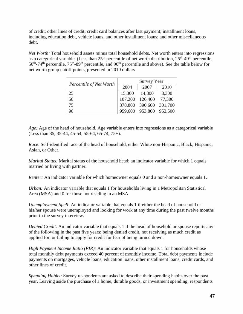
The SCF data also allow us to include other possible determinants of consumption behavior.

The level of assets and debts, as well as dummies for net worth percentiles, may impact these

choices. We can also control for the race of the head of the family, which have been shown

elsewhere to be an important factor in consumption choices (Charles et al, 2009).16

We also observe other potentially important characteristics of the family (age of the head,

marital status, number of kids) as well as an urban/non-urban classifier. Access to credit

markets, recent unemployment, and other measures of financial strain may also impact a family’s

ability to signal through spending on visible status goods. And the SCF data allow us to include

controls for families that were recently denied credit, recently experienced an unemployment

spell, or are carrying a debt burden such that debt servicing makes up more than 40 percent of

family income.17 The SCF data also allow us to measure the time that a family has spent in and

around their current residence. Specifically, we can measure the number of years that the family

head (or spouse) has lived within 25 miles of the current residence, and how recently the family

moved into their current residence.

American Community Survey Data on Neighborhood Income

The internal SCF data contain data on the state, county, and Census tract of residence for

each family. Thus, we link the SCF with summary Census tract income measures from the ACS

to help determine the income rank of each household in our sample. The 2005-2009 ACS

provides census tract level data on the overall number of households and the number of

households within 16 income buckets: less than $10,000; $10,000-$14,999; $15,000-$19,999;

$20,000-$24,999; $25,000-$29,999; $30,000-$34,999; $35,000-$39,999; $40,000-$44,999;

16 Specifically, we use indicators for households in the lowest quartile of the net worth distribution, in the 25th to 50th percentiles, the 50th to 75th percentiles, the 75th to 90th percentiles, and top decile. 17 Included among families denied credit are those who responded that they did not apply for credit because they believed they would be turned down. Earlier studies, including Jappelli (1990) and Duca and Rosenthal (1992), have found the SCF questions about credit applications and outcomes provide a useful indicator of households that are credit constrained. Krimmel, Moore, Sabelhaus, and Smith (2013) use the same 40 percent threshold to indicate risky levels of leverage among SCF households. Recent regulations given by the Consumer Financial Protection Bureau give a similar debt service-to-disposable income ratio of 43 percent in the context of regulating “qualified mortgages” (see http://files.consumerfinance.gov/f/201308_cfpb_atr-qm-implementation-guide_final.pdf).

12

$45,000-$49,999; $50,000-$59,999; $60,000-$74,999; $75,000-$99,999; $100,000-$124,999;

$125,000-$149,999; $150,000-$199,999; and $200,000 or more (in 2009 dollars).

For each household in the SCF sample, we use this tract level income distribution data to

compute the fraction of households within the tract that earns less than the sampled household—

this is a household’s income rank.18 Intuitively then, a higher income rank implies that a

household is richer relative to its neighbors.19

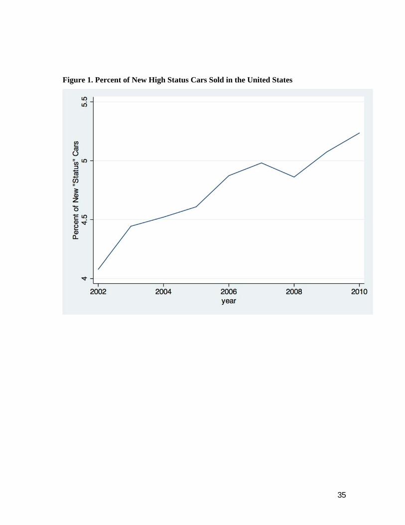
Polk Automobile Data

For each county in the United States, Polk records the number of new cars sold by make

and model. Using this information, we compute the fraction of high status cars sold in each

county over the period 2002-2010. A high status car is defined as a near-luxury or luxury car as

classified by Kelley Blue Book.20 Figure 1 shows that in the aggregate, the mean fraction of new

cars sold that were classified as high status or luxury rose steadily over the decade, from around

4.2 percent in 2002 to about 5.3 percent in 2010, with only a small drop during the financial

crisis in 2008. Table 1B reports the simple correlations between the fraction of high status cars

bought in a county and a number of demographic variables. The fraction of high status cars is

positively correlated with income inequality, as well as the median income in the county. These

cars are more likely to be bought in more urban counties and in areas with high population

density.

III. Main Results

This section presents estimates of Equation (1) using household level data from various

waves of the SCF throughout the 2000s.21 We measure status using a household’s income rank

18 Specifically, we compare the family’s normal income (found in the SCF) to the Census tract income found in the 2005-2009 ACS. Though the ACS bins reflect actual rather than permanent income groups within a census tract, the ACS is designed to be accurate over a five year period, which at least in theory abstracts transitory shocks. 19 For households with income above the $200,000 bucket, this income rank variable is potentially mis-measured. However, this affects only 2 percent of the households in our sample, and we also show that our main results are robust when income rank is measured far more coarsely as household income relative to the median income in the census tract. 20 These brands include: Acura, Aston Martin, Audi, Bentley, BMW, Cadillac, Infiniti Lamborghini, Land Rover Lexus, Lincoln, Lotus, Maserati, Maybach, Mercedes-Benz, Porsche, Rolls Royce, Tesla and Volvo. 21 Equation (1) is a linear model, though in various specification we use 5th-order polynomials of normal, which can approximate a non-parametric specification for income.

13

relative to its census tract neighbors (described above in Section IIB). This variable equals 0 if

the household’s income is in the lowest percentile, 0.1 if it is at the tenth percentile, and extends

up through 1, which indicates that the household is at the top income percentile, relative to its

neighbors in the census tract. We first examine the relationship between the household’s income

rank and various dimensions of the household’s cars. Given that the consumption, credit and

portfolio decisions are closely related, we next use the SCF to examine the relationship between

income rank on a number of credit and portfolio characteristics (Ludvigson (1999), Roussanov

(2010)).

3.1 Cars

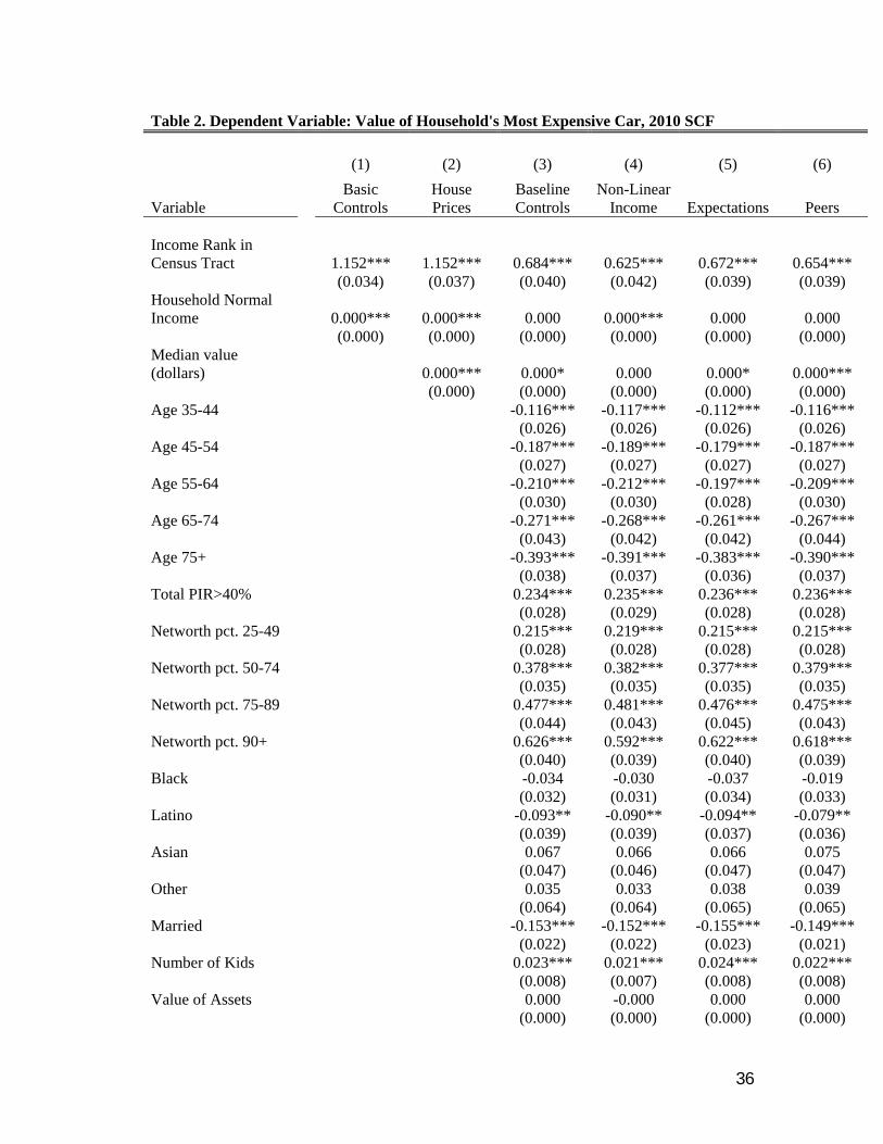
The dependent variable in Table 2 is the price of the household’s most expensive car, and

the cross-section is from the 2010 SCF. Column 1 controls linearly for the household’s “normal”

or permanent income, as well as state fixed effects to absorb state level differences in the cost of

car ownership. The coefficient on the household’s income rank is significant, positive and

economically large. A one standard deviation increase in a household’s income rank is associated

with a $4075 (or 0.41 standard deviation) increase in the value of the household’s most

expensive car.22 Even after controlling for a household’s normal income, this evidence suggests

that the household’s income relative to its neighbors might shape the consumption decision.

However, while this evidence is consistent with signaling hypothesis, the decision to locate

within a particular census tract is not random, and a number of competing explanations might

account for this association.

The cost of housing is one such explanation. Households sort into neighborhoods in part

because of local amenities like parks, schools, and access to jobs and this sorting can lead to

higher house prices in census tracts with more amenities and inelastic housing supply (Saiz

(2010)). But for those households that select into a high cost tract, the debt service burden could

also shape car buying behavior for households at different points in the income distribution,

helping to explain the results in column 1. Households for example that are poorer relative to

their neighbors in an expensive census tract could have relatively less disposable income to

invest in status goods.

22 One standard deviation in income rank is about 25 percentiles.

14

Column 2 linearly controls for the median house price in the census tract in 2010. The

results are unchanged. Available upon request are results that both linearly include this variable

and scale household income by the 2010 house price in order to compute household income

relative to the median house price in the tract. We have also used the median price in 2000—

before the housing boom and bust. In addition, the SCF also provides data on the household’s

self-reported price of the home, and in results available upon request, we also control for this

measure of house prices. In all cases, the impact of relative income on the price of the

household’s most expensive car remains large and statistically robust.

Selection into a neighborhood could be based on demographic factors that also correlate

with a household’s income rank and shape car buying behavior. Column 3 of Table 3 uses the

SCF’s household level demographic and wealth information to further control for some of these

factors. Specifically, the demographic controls include the number of children in the household;

an indicator variable for marriage; categorical variables for the age of the head of household; an

indicator variable for whether the household lives in an urban census tract; and indicator

variables for household race. We also control for a number of potentially relevant economic

variables: the value of household assets; the level of household debt; net worth is also absorbed

into a number of categorical variables; an indicator for debt service to income above the 40

percent; whether the head of household has been unemployed recently; and whether the

household has been denied credit.

These additional controls enter with intuitive signs. Households that have been turned

down for credit are more likely to buy less expensive cars, while higher net worth households are

more likely to own expensive cars. Also, some of these controls, such as the household’s debt

service, probably reflect signaling behavior itself. Households for example that purchase high

status durable goods might also have higher debt service burdens; the coefficient on debt in

column 3 is positive and significant. We consider later these alternative measures of signaling,

and column 3 likely over-controls for the joint durable good consumption-tract location decision.

By including this large number of household controls, the point estimate on income rank shrinks,

but nevertheless remains significant at the one percent level. It suggests that a one standard

deviation increase in income rank is associated with a 0.25 standard deviation increase in the

value of the family’s most expensive car.

15

Another potential confounding explanation stems from the idea that income could affect

the decision to buy a high status car non-linearly. Column 4 focuses on this possibility,

controlling for income using a fifth order polynomial. The point estimate on income rank is little

changed. Available upon request are results that model income non-parametrically within a semi-

parametric model—the results are little changed. Income expectations could also be an important

omitted variable. Households anticipating a rapid rise in future income may move into census

tracts where their current income might be well below the neighborhood’s median income; these

aspirational households may also be less able to afford a high status car, trading off the benefits

of consuming neighborhood amenities versus the ability to signal status using car ownership.

That is, rather than signaling, these results could be driven by the nexus of income

expectations and the neighborhood location decision. Fortunately, the SCF asks households both

about their income expectations and past income realizations relative to inflation. The survey

also collects data on a households’ general sentiment or optimism about the future path of the

economy. 23 These expectations are likely to shape both moving decisions and the purchase of

large consumer durables, and we include these measures of income and aggregate economic

expectations in column 5. The results are again unchanged.

There is evidence that peer effects feature in important economic decisions, and these

effects could also be a source of bias (Bertrand, Luttmer and Mullainanthan (1998), Grinblatt,

Keloharju, and Ikaheimo (2008)). Households living in areas with more high status cars might

also be induced to buy these cars, and to the extent that the percent of high status cars in the local

area is correlated with relative household income, this type of peer effect could lead to a spurious

association between relative income and status cars. Column 6 uses the Polk data to control for

the fraction of high status cars in the county bought over the past decade—we do not have this

information at the tract level. This point estimate is insignificant, and the coefficient on income

rank remains unchanged. The evidence in Coibion et. al (2014) suggests that local inequality

23 The precise questions are: X304 Over the past five years, did your total (family) income go up more than inflation, less than inflation, or about the same as inflation? X7364 Over the next year, do you expect your total (family) income to go up more than inflation, less than inflation, or about the same as inflation? X301 I'd like to start this interview by asking you about your expectations for the future. Over the next five years, do you expect the U.S. economy as a whole to perform better, worse, or about the same as it has over the past five years?

16

might matter for debt decisions, and available upon request are results that control for inequality

inside the tract; the main results remain unchanged. Available upon request are also results that

control for whether the respondent or spouse is an entrepreneur: self-employed in a partnership

or manages their own business. The results are unchanged, suggesting that they are not solely an

artifact of some types of occupational choices. In what follows we use the specification in

column 3, which controls for the potentially important household socio-economic variables as

the baseline specification.

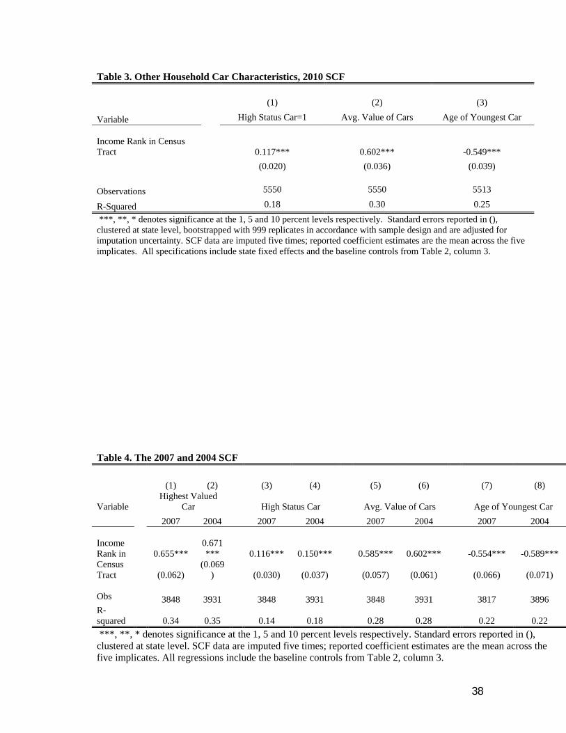
Cars can convey status and prestige along a number of different dimensions. A relatively

new car aimed at the mass market might be more expensive than a used “prestige” or “luxury”

brand car, but still signal less status than the used “prestige” brand. Similarly, owning multiple

expensive cars might be seen as an even more powerful signal of relative wealth rather than

owning a number of cars whose combined average value might be lower. Therefore, given the

nuance surrounding status indicators, Table 3 examines the impact of income rank on the car

ownership decision along some of these different dimensions, using the baseline specification

from column 3 of Table 2. Column 1 of Table 3 uses the Kelley Blue Book definitions to create

an indicator variable that equal one if the household owns a “luxury” or “near luxury” brand—a

high status car. Using the same reference data source, column 2 computes the average value of

all cars owned by the household. Column 3 focuses instead on the average age of the

household’s car.

A common pattern emerges. Income rank is positively associated with the probability of

owning a high status car and the average value of the cars owned by the household. It is also

negatively associated with the age of the household’s cars, meaning higher income-rank

households are more likely to own newer vehicles. A one standard deviation increase in income

rank implies a 3.4 percentage point rise in the probability of owning a status car; a 16.4 percent

rise in the average value of all cars; and a 15.2 percent drop in the age of the household’s

youngest car. Even along these distinct but related dimensions then, there is evidence that

relative income might affect the decision to invest in signaling goods.

Given the significant economic events over the 2000s, it would seem important to

determine whether the household level results are robust across the decade. Columns 1-8 of

Table 4 reproduce the baseline specification (column 3 of Table 2) using the 2004 and 2007 SCF

cross-sections for the four dimensions of status. The impact of relative income on these various

17

measures of status remains significant throughout, and the economic impact of income rank is

relatively stable across these disparate periods. From the 2004 SCF we see for example that a

one standard deviation increase in income rank is associated with an 18.1 percentage increase in

the value of the most expensive car. In 2007, a similar increase in relative income is associated

with a similar rise in this price.

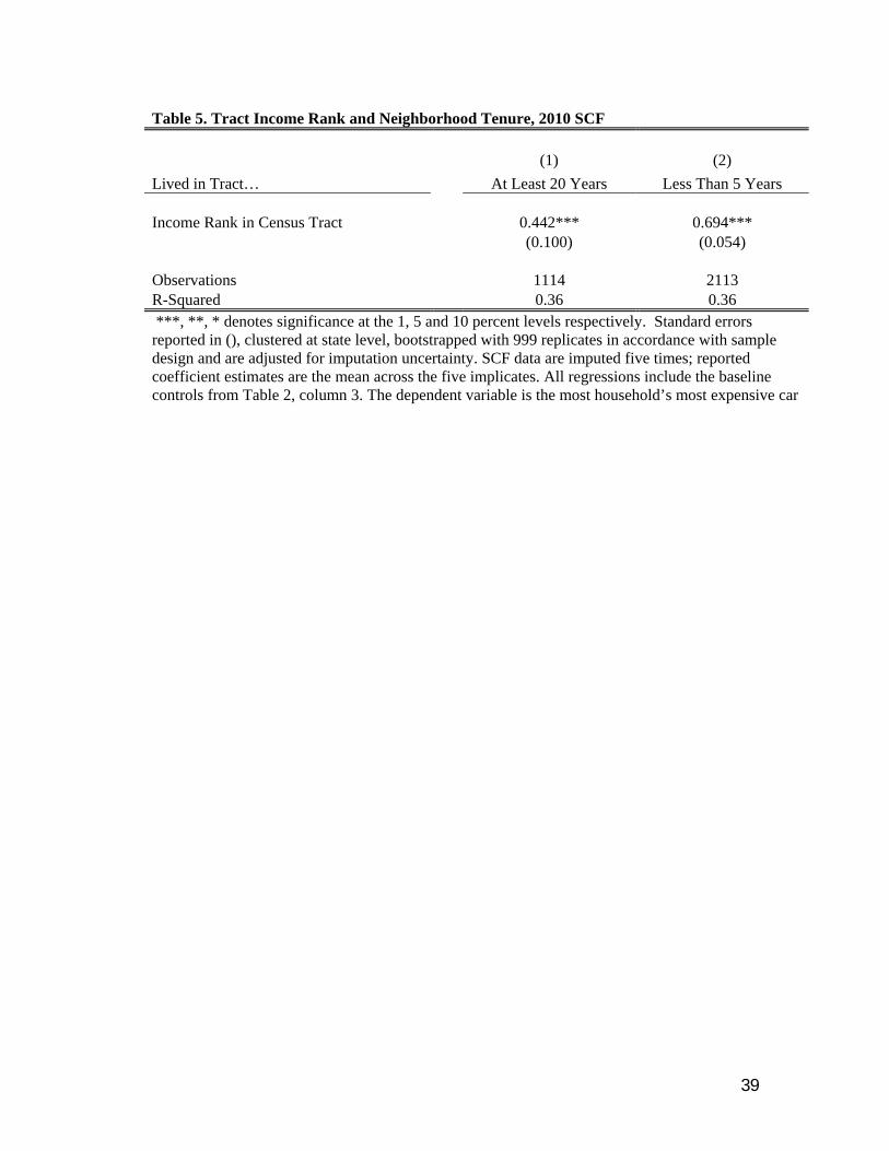
3.1.2 Tenure

Examining the length of time that a household has lived in a neighborhood—its tenure in

the neighborhood—can both help gauge the extent to which these results might be driven by

endogenous selection and also reveal better how mobility and uncertainty might shape signaling

behavior. Forecasting relative income over long periods of time can be difficult. And households

that have lived in a census tract for a long period are less likely to have selected into the tract

based on unobserved factors that determine both their relative income expectations at the time of

entry and their subsequent car buying behavior. Also, households that have lived in a

neighborhood for a long time are likely to already be part of local social networks, and may thus

have a weaker incentive to engage in costly signaling behavior.

The SCF reports how long each household has lived at its current address, and column 1

of Table 5 uses this tenure information to restrict the sample to those households that have lived

in the census tract for more than 20 years. Controlling for age and the baseline variables, the

effect of relative income remains significant, and is about two thirds the baseline estimate

reported in column 3 of Table 2; the point estimate is about the same if the sample is restricted to

those households residing in the neighborhood for more than 10 years (available upon request).

The point estimates are about 1.5 times as large when restricting the sample to only those

households that have moved into the tract within the last 5 years (column 2). Hence, for both

households that have recently moved, as well as those that are less mobile, there is evidence of

signaling behavior, suggesting that selection based on unobserved variables are unlikely to be the

principal explanation for these results.

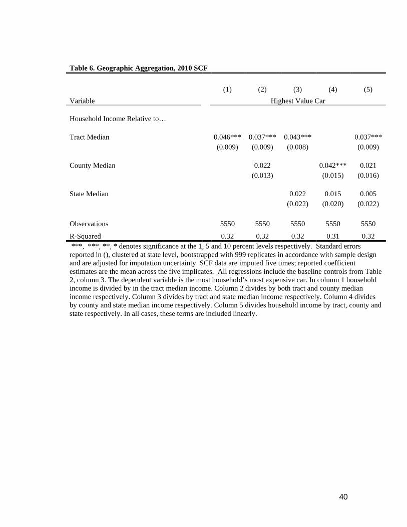
3.1.3 Measurement and Geographic Aggregation

Due to the binned nature of ACS neighborhood income data, our measurement of the

18

neighborhood income distribution may be mis-measured in the highest income tracts. As a

robustness exercise then, this sub-section considers a simpler measure of household position

within the reference group: household income relative to the tract median income.24 Using the

same baseline specification controls (column 3 of Table 2), we regress the four dimensions of

status on this relative income measure. We again find evidence that status purchases are more

likely among households with higher income relative to the median income in the tract. For

example, a one standard deviation increase in household income relative to the tract median is

associated with a 14.3 percent or 0.19 standard deviation increase in the household’s highest

valued car.

Geographically proximate neighbors are often a key reference group for most individuals,

and we have seen that relative income computed at the census tract level provides powerful

evidence of the role of signaling in consumption. However, while we have attempted to control

for a large number of household as well as tract observables, it remains possible that unobserved

factors that determine a household selection into a tract might also shape its consumption

behavior. We consider now more geographically aggregated evidence to address this concern.

The empirical strategy in Table 6 builds on the idea that while households might select

into census tracts based on relevant unobservables, selection into more aggregated political units

such as states are less likely to be affected endogenous selection. Yet households might still have

incentives to signal relative income rank at these higher levels of spatial aggregation. To be sure,

these effects are likely to be smaller since the social and economic benefits of neighborhood

networks tend to exist at more local levels.

Therefore, rather than focusing solely on relative income computed at the census tract

level (as seen in column 1), column 2 also includes a household’s income relative to the median

income in the county. Both tract-level and county-level relative income are positively associated

with the value of the household’s most expensive car. Notice, though, that the coefficient on

income relative to tract median is greater than income relative to county median in both its

economic and statistical significance. Column 3 now compares head-to-head the impact of tract

relative income to the impact of income relative to other residents in the state. We again see that

relative income at the finer geographic area dominates the higher level aggregation.

24 The model used to estimate these results also has the benefit of being similar to showing the interaction between family income and family income rank being above the median.

19

Column 4 compares county-level relative income and state-level relative income.

Finally, Column 5 considers jointly relative income computed at all three levels of spatial

aggregation. Consistent with the evidence pointing to geographically proximate neighbors as a

key reference group, a household’s relative income computed at the census tract level remains a

robust determinant of the car buying decision.

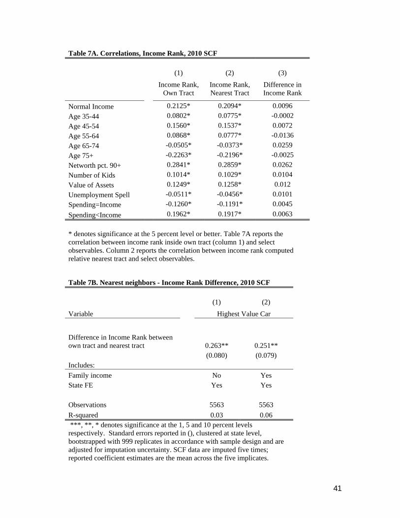
3.1.4 Nearest Neighbors

Using information on nearby neighbors can also help gauge further the extent of bias

arising from unobserved heterogeneity (Ashenfelter and Rouse (1998), Grinblatt, Keloharju and

Ikaheimo (2007)). Adjacent census tracts tend to be very similar, and households might use

consumption to signal relative income rank both to neighbors in their tract, yiOwn

, as well as to

neighbors in the nearest tract, yiNear

. Thus, using a variation of Equation (1):

(2) ci

0

1s

i

2y

iOwn

3y

iNear X

i e

i

we might expect that 3 0.

At the same time, because nearby census tracts tend to be alike, with very similar income

distributions and public goods, the potentially unobserved characteristics that might drive a

household’s decision to locate within a particular school district or political jurisdiction like a

county, could be less important when a household chooses between two adjacent tracts that offer

broadly similar amenities. This implies that the difference in a household’s income rank,

measured with respect to the income distribution in its own tract, as well as the nearest tract, is

unlikely to be uncorrelated with unobserved household characteristics that determine

neighborhood selection:

(3) yiOwn

yiNear

vi, where cov(v

i,e

i) 0

Therefore, this difference yiOwn yiNear can provide a conservative, though potentially noisy

estimate of the importance of status.

20

While it is not possible to formally test the assumption that cov(vi,e

i) 0, the basic

correlations in Table 7A lend some plausibility to this idea. Consistent with the fact that

household characteristics are related to neighborhood selection, a household’s income rank

relative to the income distribution in its own census tract is highly correlated with the

household’s income level, net worth, age categories, race, debt, and even its savings decision.

Moreover, in keeping with the idea that the nearest census tract is likely to be perceived by

households as offering similar amenities, column 2 shows that the correlations between

household observables and income rank measured with respect to the nearest census tract are

nearly identical to column 1. For example, the correlation between normal income and income

rank measured either with respect to the household’s own tract or the nearest tract is identical.

Interestingly, the difference in income rank across the two tracts (column 3) is uncorrelated with

these key predictors of neighborhood selection, suggesting that indeed, the difference in income

rank might be unrelated to the unobservables that drive selection.

Table 7B shows that this difference in income rank is significantly correlated with the

price of the household’s most expensive car. These results are less precise than those obtained

earlier, but the point estimate in column 1 suggests that a one standard deviation increase in the

differenced income rank is associated with a 3.1 percent increase in the price of the household’s

most expensive car. Adding normal income does little to change the point estimate (column 2),

while adding the full panoply of controls leads to greater imprecision, but there is little change in

the point estimate (available upon request).25

3.2. Credit and Portfolio Decisions

We have seen evidence that income rank might shape a household’s decision to spend

more on cars in order to signal status. However, cars are expensive durable goods that are often

bought on credit, and we might expect to see evidence of this signaling behavior in household

credit decisions (Benmelech, Meisenzahl and Ramcharan (2014)). In addition, concerns about

25 Our robustness checks also included comparing the base model in tables 2 and 3 to a model which completely excludes income rank (which corresponds to a general neoclassical model of consumption). The R2 is 0.31 in the model excluding income rank, 0.03 lower than the R2 in the model which includes income rank (0.34; see column 3 of table 2). Thus, income rank adds explanatory power to a model of conspicuous consumption. Further, in the base model (column 3 of table 2), the unobservable components of owning a car of high value are balanced across the deciles of income rank.

21

relative status might help explain the heterogeneity in risky assets across household portfolios, as

households seeking to “get ahead of the Joneses” or those that care about status associated with

absolute wealth might hold riskier portfolios (Caroll (2002), Roussanov (2010)). In this

subsection then, we make use of the richness of the SCF to analyze the role of status on these

household decisions.

3.2.1 Credit

The results in Table 8 mirror those obtained using cars. The dependent variable in

column 1 is the average household credit card balance, while column 2 focuses on the

household’s overall debt payments. In both instances, there is robust evidence that these

variables are positively related to income rank. A one standard deviation increase in income rank

is associated with a 0.15 standard deviation increase in credit card balances (column 1); and a

0.27 standard deviation increase in overall debt payments (Table 8, column 2). Consistent with

the idea the households with more credit card debt are more likely to file for bankruptcy, income

rank is also positively associated with whether the household has ever filed for bankruptcy

(Domowitz and Sartain (1999)). A one standard deviation increase in income rank implies a 1.3

percentage point increase in the probability that the household has filed for bankruptcy (column

3). Thus, although auto loans are collaterized and repossessed in bankruptcy proceedings, and are

unlikely to influence directly the decision to file for bankruptcy, this pattern of evidence suggests

that consumers may use unsecured credit to buy invest more broadly in visible status goods (Fay,

Hurst and White (2002)).

3.2. Portfolio Heterogeneity

To investigate whether status considerations might also explain the heterogeneity in

portfolio riskiness across households, column 1 of Table 9 uses the share of household total

equities to the value of household total financial assets as the dependent variable. It is well

known that wealthier households tend to have riskier portfolios and we continue to control for

the baseline demographic and economic variables (Table 2, column 3), including household net

worth. Consistent with the idea that concerns about status might induce households to hold more

risky assets, the coefficient on income rank is positive and significant at the one percent level. It

22

suggests that a one standard deviation increase in income rank is associated with a 4.6 percentage

point or 0.14 standard deviation rise in the share of equity in the household’s portfolio.

Unobserved attitudes to risk taking might drive these portfolio decisions and also increase

a household’s income relative to its neighbors. The SCF directly asks households about their risk

preferences.26 And we include answers to these questions in column 2. A determined skeptic may

dismiss the value of these survey based questions. There is however some evidence that survey

responses are correlated with economic choices (Puri and Robinson (2007)), and from column 2,

households claiming to take substantial risks for substantial returns do hold significantly more

equity relative to households claiming to be less risk tolerant. The point estimate on income rank

decreases slightly, but remains significant at the one percent level.

In addition to riskier portfolios, social status concerns and the desire to “get ahead of the

Joneses” might also prompt some households to concentrate in activities with idiosyncratic

payoffs, such as entrepreneurship (Roussanov (2010)). The SCF asks whether the survey

respondent or spouse is an entrepreneur: self-employed in a partnership or manages their own

business. Consistent with the idea that social status concerns might drive risk taking, from

column 3, there is a significant positive association between the probability that a household is

involved in entrepreneurship and its relative income rank. We continue to control for self-

reported risk attitudes, but it remains possible that unobserved risk attitudes could explain these

results. We now focus further on these concerns.

3.3 Unobserved Heterogeneity and the SCF Panel

Despite the persistence of these results across a number of very different specifications, it

remains possible that the positive association between income rank and the consumption of

status automobiles along with credit and portfolio decisions might be an artifact of unobserved

factors that determine both selection into a census tract and household behavior. In this

subsection, we make use of the 2007-2009 SCF panel in order to develop tests that can control

26 The question is “Which of the statements on this page comes closest to the amount of financial risk that you (and your {husband/wife/partner}) are willing to take when you save or make investments? 1. *Take substantial financial risks expecting to earn substantial returns. 2. *Take above average financial risks expecting to earn above average returns. 3. *Take average financial risks expecting to earn average returns. 4. *Not willing to take any financial risks.

23

for time invariant household preferences. This special panel unfortunately does not ask detailed

questions on car ownership, but it includes the standard credit variables, as well as the portfolio

measure from Table 9. Column 1 of Table 10 presents the results from regressing the log total

household debt payments over this period on income rank, normal income, household assets, and

variables that indicate whether the household experienced a change in marital status, number of

children, or whether the household moved. Race and the other time invariant controls are

absorbed in the household fixed effect.

From column 1, a one standard deviation increase in income rank is associated with a

0.08 standard deviation increase in total debt payments.27 Rather than focusing on debt service,

column 2 uses debt stock as the dependent variable. The coefficient on income rank is positive

and significant at the 5 percent level. Column 3 excludes housing debt, and again there is

evidence that household credit usage might be driven by relative status considerations. But non-

housing debt might still include student loans and other non-consumption related expenditures,

and column 4 uses log credit card debt as the dependent variable. A one standard deviation

increase in income rank is associated with a 0.26 standard deviation increase in credit card debt.

Column 5 uses the share of equity in household total financial assets as the dependent

variable. To the extent that risk preferences are time invariant, the panel estimates are unlikely to

biased by these unobserved factors. We again find evidence of a positive association between

income rank and portfolio risk taking, after controlling for household fixed effects. Taken

together, these various pieces of evidence suggest that heterogeneity in income rank might be a

significant factor in shaping a household’s consumption, credit and portfolio decisions. In the

next sub-section, we explore some potential aggregate implications of these findings.

V. Aggregate Evidence

The household level evidence suggests that if we treat the county as the relevant

geographic unit of analysis, then models that emphasize the importance of status would predict

that in a cross-section of counties, the demand for high status cars should be higher in counties

with a greater dispersion in incomes. In contrast, in counties where incomes are known to be

more homogenous, communicating information about status is likely to be less important in the

27 One standard deviation in income rank is approximately two deciles.

24

decision to buy a car, and the demand for high status cars in those counties should be smaller. In

this subsection, we consider this prediction, examining the impact of inequality within a county

on the fraction of high status cars bought in that county.

Polk gives us the make and model for each car sold in the county and we use Kelley Blue

Book’s definition of near luxury and above models to identify high status cars, computing the

ratio of high status to total cars sold in the county within a calendar year as our dependent

variable of interest. We observe these data annually from 2002-2010. The inequality and other

county level observables are available at two points in time: From the US Census in 2000 and

from the ACS in 2005-2009. The ACS data are sampled over the period 2005-2009 and is

considered accurate over this sampling period. The empirical strategy matches the Polk data over

the period 2002-2004 with the 2000 Census, and uses the ACS data for the 2005-2009 period.28

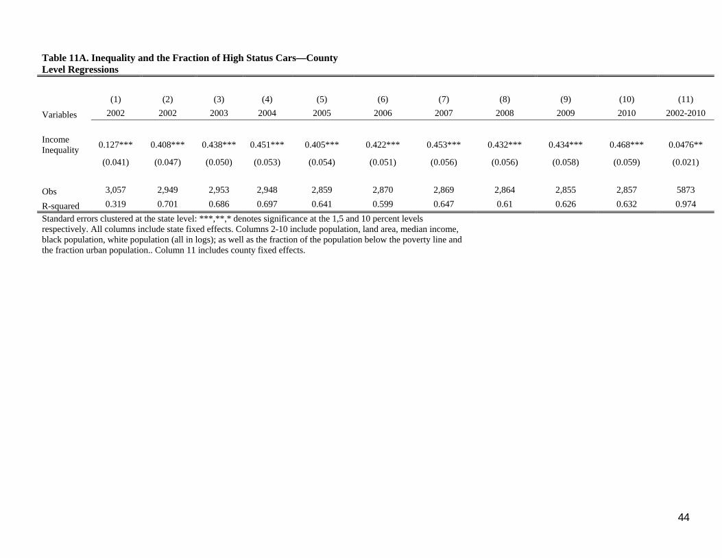
Column 1 of Table 11A regresses the high status ratio, observed in 2002, on the Gini

coefficient in the county computed from the 2000 Census. State fixed effects, which controls for

potentially important state level factors like the state gas tax and other state government imposed

costs on car ownership, such as registration fees and emission requirements, are the only

additional controls. The Gini point estimate is statistically and economically significant,

suggesting that a one standard deviation increase in inequality is associated with a 0.4 percentage

point or 0.16 standard deviation increase in the fraction of high status cars purchased in the

county.

Column 2 controls for a number of potentially important socio-economic factors. The

fraction of high status cars are likely to be higher in richer counties, and we control for both the

log of median income in the county as well as the fraction of residents below the poverty line.

Demographic factors like the log population, area, urbanization and the racial composition of the

county are also likely to be important. These variables enter with intuitive signs. A one standard

deviation increase in median income is associated with a 0.53 standard deviation increase in the

fraction of high status cars bought in the county; these types of cars are also less likely to be

28 Note that the 2004, 2007, and 2010 SCF surveys use the 2000 decennial Census definitions of tract borders. The 2005-2009 is the only ACS data that use the 2000 Census tract definitions and have statistics at the Census tract level. Gini coefficient data used in our analysis at the county level come from the 2006-2010 ACS because the 2005-2009 ACS does not have county level Gini data and county definitions do not change each decade. All ACS data and subsequent results are presented in inflation-adjusted 2010 dollars to remain consistent with the 2010 SCF cross section.

25

purchased in more urban, and presumably more congested counties. The coefficient on inequality

is about double that in column 1 and remains significant at the one percent level.

Columns 3-10 repeat this exercise for the period 2003-2010. This period spans both the

boom in consumption and house prices, the rise of securitization in auto-financing and the

extension of subprime credit, the financial crisis and the Great Recession. Recall that for 2005-

2010 the county level data are drawn from the ACS. Despite these differences across the sample

period, the impact of inequality on the ratio of high status cars bought in the county remains

significant and is largely unchanged.

While the county-level evidence helps gauge the potential aggregate impact of the status

motive on consumption, it also raises a number identification challenges not present in the more

detailed household level data. In the presence of credit market frictions, rising inequality could

for example disproportionately limit credit access for those at the bottom of the income

distribution, leading to a large bifurcation in the types of cars bought inside a highly unequal

county. Apart from credit market frictions, car purchases are often amortized over a number of

years, and differences in expectations of income growth for those at different points in the

income distribution could also explain these results. Likewise, micro targeted advertising that

steer some buyers to certain brands could also help account for some these results.

It is also possible that county time invariant factors, such as the local industrial structure,

perhaps as determined by weather or local geography, might both drive inequality and the types

of cars available for purchase in a county, helping to explain some of these results. Also, the

historic location of car dealership networks could also affect the supply of certain types of luxury

models, leading to a potentially spurious association between inequality and the fraction of high

status cars bought in a county. That is, many high status cars are imported, with well-developed

dealership and parts distribution networks along the coasts, lowering the cost of ownership. At

the same time, economic activity and migration patterns along the coasts could independently

lead to a more unequal income distribution in those areas, inducing a positive relationship

between inequality and the fraction of high status cars that is unrelated to the signaling

hypothesis.

To address some of these concerns, column 11 constructs a panel based on the US Census

and ACS data, allowing the use of county level fixed effects to absorb non-parametrically these

potentially important time invariant factors. We average the status ratio over the two sub-periods

26

2002-2004 and 2005-2010, and then regress the change in the ratio of high status cars over these

two periods on the change in inequality and the other covariates. At this level of spatial

disaggregation, both inequality and the ratio of high status cars are highly persistent. In the case

of the former, the correlation across the two periods is 0.69 at the county level, while in the case

of high status cars the correlation is 0.94. Also, including county fixed effects absorbs some of

the mediating mechanisms, such as culture and social norms, through which inequality might

affect signaling behavior. Despite these factors, the evidence in column 11 continues to suggest

that an increase in inequality within a county is significantly associated with an increase in the

ratio of high status cars. The point estimate implies that a one standard deviation increase in

inequality is associated with a 0.06 standard deviation rise in the ratio of high status cars.

We now exploit some of the historic determinants of inequality to gauge further the

robustness of these results. This approach is motivated by the fact there is already substantial

evidence both in the United States and elsewhere that some economic and social forces can be

highly persistent. For example, segregation changed dramatically over the 20th century, yet

Cutler, Glaeser and Vigdor (1999) show that the relative segregation of different cities remained

highly persistent, with the correlation across cities between segregation in 1890 and segregation

in 1990 as high as 50 percent. In like vein, Acemoglu, Johnson and Robinson (2001) and

Engerman and Sokoloff (2002) provide international evidence on the persistence of important

economic and political institutions. Building on these ideas, we instrument county level

inequality averaged over 2002-2010 with the inequality in farm holdings observed in 1920.

Counties with more unequal farm holdings in the early 20th century tended to spend far

less on education and other redistributive public goods, and there is evidence that elites in these

counties were better able to use their relative political power to restrain both the provision of

public goods and financial development (Ramcharan (2010), Rajan and Ramcharan (2011,

2014). Less public redistribution and more limited access to private credit are both likely to limit

social mobility, and lead to persistent inequality within a county (Galor, Moav and Vollrath

(2008)).

Interesting in its own right, the first stage regression in column 1 of Table 11B supports

the idea that while the US has experienced substantial social and economic change over time, the

cross-sectional variation inequality remains highly persistent.29 Column 1 uses the Gini

29 The correlation coefficient between expenditures per pupil at the county level in 1920 and 1994 is 0.92.

27

coefficient of income inequality averaged over 2002-2010 as the dependent variable, and

conditions on the standard suite of demographic and economic controls, as well as state fixed

effects. The point estimate on the Gini coefficient of farm holdings in 1920 is positive and

significant at the one percent level. A one standard deviation increase in this variable is

associated with a 0.08 standard deviation increase in income inequality averaged over 2002-

2010.

Column 2 of Table 11B regresses the fraction of high status cars sold in the county

averaged over 2002-2010 on contemporary inequality, with the latter instrumented using land

inequality in 1920. Exploiting the variation in farm land inequality from 1920—a period that

largely predates the expansion of the automobile—the IV point estimate is statistically

significant at the one percent level and large. A one standard deviation increase in contemporary

inequality is associated with a 0.67 standard deviation increase in the fraction of high status cars

sold over the decade; this magnitude is slightly larger than the corresponding OLS estimate

reported in column 3.

We have already seen household evidence linking the signaling hypothesis to the use of

consumer credit. Using data on the median household leverage ratio for 2006 in each county

(Mian and Sufi (2011), we examine this prediction at the county level. The point estimate is

positive and significant at the one percent level, and suggests that a one standard deviation

increase in inequality is associated with a 0.10 standard deviation increase in household leverage

within the county (column 4). Unobserved factors that increase inequality, like limited access to

credit, could also lead to lower leverage, and these estimates could be biased downwards. The IV

point estimate in column 5, which uses the historic variation in inequality, is about 10 times

larger. This evidence strongly suggests that the dispersion incomes might matter for the

consumption of luxury goods.

IV. Conclusion

This paper has investigated the importance of the status concerns in the consumption and

financial decisions of households. Using the SCF linked with Census tract information from the

ACS, we find evidence that a household’s income rank relative to its close neighbors—those in

28

the same census tract—is positively associated with the decision to buy a high status car. After

controlling for income itself, as well as a number of other demographic and economic variables,

income rank is also positively associated with credit usage, including credit card balances, the

decision to file for bankruptcy, and riskier portfolios. The aggregate county-level evidence also

appears consistent with the signaling hypothesis. Income inequality at the county-level is

positively associated with both the fraction of high status cars bought in the county, and

indicators of consumer leverage. These results suggest the signaling motive might feature in

some durable goods consumption choices, as households seek to “get ahead of the Joneses”, and

invest in status consumption goods to signal that they might have advanced in their relative

income position. These findings also suggest that rising inequality might have broader

macroeconomic consequences, including a reduced savings rate and greater household debt.

29

References

Abel, Andrew. 1990. “Asset prices under habit formation and catching up with the Joneses” American Economic Review, 80, 38-42.

Acemoglu, Daron and Robinson, James. 2011. “Why Nations Fail: The Origins of Power, Prosperity and Poverty. Crown Publishing Group

Ait-Sahalia, Yacine, Jonathan Parker, Motohiro Yogo. 2004. “Luxury Goods and the Equity Premium.” : 1–46. Journal of Finance

Ashenfelter, Orley and Cecilia Rouse. 1998. “Income, Schooling, and Ability: Evidence from a New Sample of Identical Twins”, Quarterly Journal of Economics, 113, 253-84.

Bagwell, L S, and B D Bernheim. 1996. “Veblen effects in a theory of conspicuous consumption.” American Economic Review: 349–373.

Becker, Gary S, Kevin M Murphy, and Ivan Werning. 2005. “The Equilibrium Distribution of Income and the Market for Status.” Journal of Political Economy 113(2): 282–310.

Bertrand, Marianne, Erzo F P Luttmer, and Sendhil Mullainathan. 1998. Network effects and welfare cultures.

Bertrand, Marianne and Adair Morse. 2013. “Trickle-Down Consumption”, NBER Working Paper No. 18883

Bliege Bird, R. and Smith, E. A. (2005) “Signaling Theory, Strategic Interaction, and Symbolic Capital'', Current Anthropology, 46, Bliege Bird, R., Smith, E. A. and Bird, D. W. (2001) “The Hunting Handicap: Costly Signaling in Human Foraging Strategies'', Behavioral Ecology and Sociobiology 50

Bricker, Jesse, Arthur Kennickell, Kevin Moore, and John Sabelhaus (2012) “Changes in U.S. Family Finances from 2007 to 2010: Evidence from the Survey of Consumer Finances,” Federal Reserve Bulletin, Vol. 98, No. 2, pp. 1–80.

Borjas, George J. ‘‘Ethnicity, Neighborhoods, and Human-Capital External- ities.’’ American Economic Review, 85 ( June 1995): 365–90.

Campbell, John Y. 2006. “Household Finance.” The Journal of Finance 61(4): 1553–1604.

Campbell, John and Cochrane, John. 1999. “By Force of Habit: A consumption based Explanation of Aggregate Stock Market Behavior”, Journal of Political Economy,

30

107, 205-251.

Card, David, Alexandre Mas, Enrico Moretti, and Emmanuel Saez. 2012. “Inequality at Work: the Effect of Peer Salaries on Job Satisfaction.” American Economic Review 102(6): 2981–3003.

Charles, K, E Hurst, and N Roussanov. 2009. “Conspicuous consumption and race.” The Quarterly Journal of Economics 124(2): 425–467.

Coibion, Olivier, Yuriry Gorodnichenk, Marianna Kudlyak and John Mondragon. “Does Inequality Lead to More Household Borrowing? New Evidence from Household Data”. 2014.

Cronk, L. 2005. “The application of animal signaling theory to human phenomena: some thoughts and clarifications.” Social Science Information 44(4): 603–620.

Cutler, David M, Edward L Glaeser, and Jacob L Vigdor. 1999. “The Rise and Decline of the American Ghetto.” Journal of Political Economy 107(3): 455.

DeMarzo, Peter, Ron Kaniel and Ilan Kremer, 2004, Diversification as a public good: Community effects in portfolio choice, Journal of Finance 59, 1677-1715.

Duca, John, and Stuart Rosenthal (1991) “An Econometric Analysis of Borrowing Constraints and Household Debt,” Federal Reserve Bank of Dallas Research Paper No. 9111.

Dupor, Bill, and Wen-Fang Liu. 2003. “Jealousy and Equilibrium Overconsumption.” American Economic Review 93(1): 423–28.

Duesenberry, James S., 1949, Income, Saving, and the Theory of Consumer Behavior (Harvard University Press, Cambridge, MA).

Frank, R H. 1985. “The demand for unobservable and other nonpositional goods.” American Economic Review 75(1): 101–116.

Frank, R H. 1989. “Frames of Reference and the Quality of Life.” American Economic Review 79(2): 80–85.

Glaeser, E, and D Cutler. 1997. “Are ghettos good or bad?.” Quarterly Journal of Economics 112(3): 827–872.

Glazer, A, and K A Conrad. 1996. “A signaling explanation for charity.” American Economic Review 86(4): 1019–1028.

Grinblatt, Mark, and Matti Keloharju. 2001. “How Distance, Language, and Culture Influence Stockholdings and Trades.” The Journal of Finance 56(3): 1053–73.

Grinblatt, Mark, Matti Keloharju and Seppo Ikaheimo. 2008. “Social Influence and

31

Consumption: Evidence From the Automobile Purchases of Neighbors”, Review of Economics and Statistics, November, 90(4): 735-753.

Han, Young Jee, Joseph C Nunes, and Xavier Drèze. 2010. “Signaling Status with Luxury Goods: the Role of Brand Prominence.” Journal of Marketing 74(4): 15–30.

Heffetz, O. 2011. “A test of conspicuous consumption: Visibility and income elasticities.” Review of Economics and Statistics 93(4): 1101–1117.

Hong, Harrison, Jeffrey D. Kubik, and Jeremy C. Stein, 2003, Social interaction and stock market participation, Journal of Finance 59, 137–163.

Jappelli, Tulio (1990). “Who is Credit-Constrained in the U.S. Economy?” Quarterly Journal of Economics, 105(420): pp. 219–234.

Kennickell, Arthur (2001) “Modeling Wealth with Multiple Observations of Income: Redesign of the Sample for the 2001 Survey of Consumer Finances” In Proceedings of the Survey Research Section of the American Statistical Association.

Kennickell, Arthur (1998) “List Sample Design for the 1998 Survey of Consumer Finances” Federal Reserve Board mimeo.

Kennickell, Arthur and Douglas McManus (1993) “Sampling for Household Financial Characteristics Using Frame Information on Past Income” Federal Reserve Board mimeo.

Koszegi, B, and M Rabin. 2007. “Reference-dependent risk attitudes.” American Economic Review 97(4): 1047–1073.

Krimmel, Jacob, Kevin B. Moore, John Sabelhaus, and Paul Smith (2013). "The Current State of U.S. Household Balance Sheets," Federal Reserve Bank of St. Louis Review, vol. 95, no. 5, pp. 337-359.

Loewenstein, G, T O’Donoghue, and M Rabin. 2003. “Projection bias in predicting future utility.” The Quarterly Journal of Economics 118(4): 1209–1248.

Luttmer, F P. “Erzo (2005), Neighbors as negatives: relative earnings and wellbeing.” Quarterly Journal of Economics 120: 963. Piketty, Thomas. 2014. Capital in the Twenty First Century. Harvard University Press. Puri, Manju and David Robinson. 2007. “Optimism and Economic Choice”, Journal of Financial Economics, vol. 86(1). Rajan, Raghuram G, and Rodney Ramcharan. 2011. “Land and Credit: a Study of the Political Economy of Banking in the United States in the Early 20th Century.” The Journal of Finance 66(6): 1895–1931.

32

Rajan, Raghuram G. 2010. Fault Lines: How Hidden Fractures Still Threaten the World Economy. Princeton University Press. Ramcharan, Rodney. 2010. “Inequality and Redistribution: Evidence From US Counties and States, 1890-1930.” Review of Economics and Statistics 92(4): 729–44. Rhode, Paul W., and Koleman S. Strumpf, “Assessing the Importance of Tiebout Sorting: Local Homogeneity from 1850 to 1990,” American Economic Review 93 (2003), 1648–1677.

Roussanov, Nikolai. 2010. “Diversification and Its Discontents: Idiosyncratic and Entrepreneurial Risk in the Quest for Social Status.” The Journal of Finance 65(5): 1755–88. Sundie, Jill M, Douglas T Kenrick, Vladas Griskevicius, Joshua M Tybur, Kathleen D Vohs, and Daniel J Beal. 2011. “Peacocks, Porsches, and Thorstein Veblen: Conspicuous Consumption as a Sexual Signaling System..” Journal of Personality and Social Psychology 100(4): 664–80. Tourangeau, Roger, Robert Johnson, Jiahe Qian, Hee-Choon Shin, and Martin Frenkel

(1993) “Selection of NORC’s 1990 National Sample” National Opinion Research Center at the University of Chicago working paper.

Veblen, Thorstein, The theory of the leisure class: an economic study of institutions, (1899).

33

Tables and Figures Table 1A. SCF summary statistics

2004 2007 2010

Age: Percent of family heads… Age < 35 0.21 0.21 0.19 Age 35-44 0.21 0.20 0.19 Age 45-54 0.21 0.21 0.22 Age 55-64 0.16 0.18 0.18 Age 65-74 0.11 0.11 0.11 Age > 75 0.10 0.09 0.10 Net worth Percentiles: Percent of families in… Networth pct < 25 0.20 0.20 0.19 Networth pct. 25-49 0.26 0.26 0.26 Networth pct 50-74 0.27 0.27 0.27 Networth pct 75-89 0.16 0.16 0.16 Networth pct >=90 0.11 0.11 0.11 Race/Ethnicity: Percent of family heads… White 0.77 0.76 0.74 Black 0.11 0.11 0.12 Latino 0.09 0.09 0.10 Asian 0.02 0.03 0.03 Other 0.01 0.01 0.01 Pct. married 0.63 0.64 0.63 Avg. num of kids 0.84 0.86 0.88 Pct. Renter 0.26 0.26 0.27 Pct urban 0.82 0.82 0.82 Pct with recent unemp spell 0.16 0.14 0.21 Pct denied credit 0.22 0.20 0.25 Pct with high PIR (>40 pct) 0.10 0.12 0.11 Pct entrepreneur 0.19 0.17 0.18 Pct equity in total financial assets 0.31 0.32 0.28 Spending: percent where spending… Exceeded income 0.15 0.15 0.16 Equaled income 0.26 0.26 0.29 Less than income 0.59 0.59 0.54 Means of… Normal income 87,225 90,655 89,780 Assets 655,195 728,056 641,622 Debts 98,933 109,776 106,505 Tract Median Housing Value (via ACS) 254,763 243,605 246,923 Tract Median Income (via ACS) 58,980 58,635 58,526 Household Within-Tract Income Rank 0.54 0.53 0.54 Household Income Relative to Tract Median 1.45 1.49 1.47

34

Note: Weighted means of SCF demographic variables. Variables in this table are those of the main regression model (col. 3 of table 2), plus select variables used in other regressions. As such, these summary statistics represent car-owning families.

Table 1B. Fraction of High Status Cars: County-level correlations, 2002-2010

(1) Variables 2002-2010 Population Density 0.39 Urban population (percent) 0.41 Median income 0.51 Gini Coefficient 0.28 Poverty Rate -0.15 Black population (percent) 0.22

This table reports the correlations between the average fraction of high status cars bought in county (2002-2010) and select county demographic variables. All correlations are significant at the one percent level.

35

Figure 1. Percent of New High Status Cars Sold in the United States

36

Table 2. Dependent Variable: Value of Household's Most Expensive Car, 2010 SCF (1) (2) (3) (4) (5) (6)

Variable Basic

Controls House Prices

Baseline Controls

Non-Linear Income Expectations Peers

Income Rank in Census Tract 1.152*** 1.152*** 0.684*** 0.625*** 0.672*** 0.654*** (0.034) (0.037) (0.040) (0.042) (0.039) (0.039) Household Normal Income 0.000*** 0.000*** 0.000 0.000*** 0.000 0.000 (0.000) (0.000) (0.000) (0.000) (0.000) (0.000) Median value (dollars) 0.000*** 0.000* 0.000 0.000* 0.000*** (0.000) (0.000) (0.000) (0.000) (0.000) Age 35-44 -0.116*** -0.117*** -0.112*** -0.116*** (0.026) (0.026) (0.026) (0.026) Age 45-54 -0.187*** -0.189*** -0.179*** -0.187*** (0.027) (0.027) (0.027) (0.027) Age 55-64 -0.210*** -0.212*** -0.197*** -0.209*** (0.030) (0.030) (0.028) (0.030) Age 65-74 -0.271*** -0.268*** -0.261*** -0.267*** (0.043) (0.042) (0.042) (0.044) Age 75+ -0.393*** -0.391*** -0.383*** -0.390*** (0.038) (0.037) (0.036) (0.037) Total PIR>40% 0.234*** 0.235*** 0.236*** 0.236*** (0.028) (0.029) (0.028) (0.028) Networth pct. 25-49 0.215*** 0.219*** 0.215*** 0.215*** (0.028) (0.028) (0.028) (0.028) Networth pct. 50-74 0.378*** 0.382*** 0.377*** 0.379*** (0.035) (0.035) (0.035) (0.035) Networth pct. 75-89 0.477*** 0.481*** 0.476*** 0.475*** (0.044) (0.043) (0.045) (0.043) Networth pct. 90+ 0.626*** 0.592*** 0.622*** 0.618*** (0.040) (0.039) (0.040) (0.039) Black -0.034 -0.030 -0.037 -0.019 (0.032) (0.031) (0.034) (0.033) Latino -0.093** -0.090** -0.094** -0.079** (0.039) (0.039) (0.037) (0.036) Asian 0.067 0.066 0.066 0.075 (0.047) (0.046) (0.047) (0.047) Other 0.035 0.033 0.038 0.039 (0.064) (0.064) (0.065) (0.065) Married -0.153*** -0.152*** -0.155*** -0.149*** (0.022) (0.022) (0.023) (0.021) Number of Kids 0.023*** 0.021*** 0.024*** 0.022*** (0.008) (0.007) (0.008) (0.008) Value of Assets 0.000 -0.000 0.000 0.000 (0.000) (0.000) (0.000) (0.000)

37

Table 2, Cont’d.

Household Debt 0.000*** 0.000*** 0.000*** 0.000*** (0.000) (0.000) (0.000) (0.000) Unemployment Spell -0.165*** -0.163*** -0.157*** -0.164*** (0.016) (0.016) (0.016) (0.017) Turned Down for Credit -0.075*** -0.075*** -0.072*** -0.075*** (0.024) (0.024) (0.025) (0.024) Spending=Income -0.063** -0.063** -0.066** -0.063** (0.031) (0.031) (0.031) (0.031) Spending<Income 0.036 0.033 0.027 0.037 (0.033) (0.033) (0.034) (0.033) Urban -0.016 -0.016 -0.010 -0.048* (0.027) (0.027) (0.028) (0.028) Renter -0.093*** -0.089*** -0.092*** -0.090*** (0.029) (0.028) (0.028) (0.028) Fraction of High Status Cars in County -0.912*** (0.253) Past Income Grew<Inflation -0.092*** (0.028) Past Income Grew=Inflation -0.050* (0.028) Future Income Grow<Inflation 0.049* (0.025) Future Income Grow=Inflation 0.050** (0.022) Economy will get worse -0.019 (0.029) Economy will stay same -0.034* (0.019) Observations 5585 5550 5550 5550 5550 5550 R-squared 0.21 0.24 0.34 0.34 0.34 0.34 ***, **, * denotes significance at the 1, 5 and 10 percent levels respectively. Standard errors reported in (), clustered at state level, bootstrapped with 999 replicates in accordance with sample design and are adjusted for imputation uncertainty. SCF data are imputed five times; reported coefficient estimates are the mean across the five implicates. Column 4 includes normal income as a fifth order polynomial—terms not shown for concision. All specifications include state fixed effects.

38

Table 3. Other Household Car Characteristics, 2010 SCF

(1) (2) (3)

Variable High Status Car=1 Avg. Value of Cars Age of Youngest Car

Income Rank in Census Tract 0.117*** 0.602*** -0.549***

(0.020) (0.036) (0.039)

Observations 5550 5550 5513

R-Squared 0.18 0.30 0.25

***, **, * denotes significance at the 1, 5 and 10 percent levels respectively. Standard errors reported in (), clustered at state level, bootstrapped with 999 replicates in accordance with sample design and are adjusted for imputation uncertainty. SCF data are imputed five times; reported coefficient estimates are the mean across the five implicates. All specifications include state fixed effects and the baseline controls from Table 2, column 3.

Table 4. The 2007 and 2004 SCF

(1) (2) (3) (4) (5) (6) (7) (8)

Variable Highest Valued

Car High Status Car Avg. Value of Cars Age of Youngest Car

2007 2004 2007 2004 2007 2004 2007 2004 Income Rank in Census Tract

0.655*** 0.671*** 0.116*** 0.150*** 0.585*** 0.602*** -0.554*** -0.589***

(0.062) (0.069

) (0.030) (0.037) (0.057) (0.061) (0.066) (0.071) Obs 3848 3931 3848 3931 3848 3931 3817 3896 R-squared

0.34 0.35 0.14 0.18 0.28 0.28 0.22 0.22

***, **, * denotes significance at the 1, 5 and 10 percent levels respectively. Standard errors reported in (), clustered at state level. SCF data are imputed five times; reported coefficient estimates are the mean across the five implicates. All regressions include the baseline controls from Table 2, column 3.

39

Table 5. Tract Income Rank and Neighborhood Tenure, 2010 SCF (1) (2)

Lived in Tract… At Least 20 Years Less Than 5 Years Income Rank in Census Tract 0.442*** 0.694*** (0.100) (0.054) Observations 1114 2113 R-Squared 0.36 0.36 ***, **, * denotes significance at the 1, 5 and 10 percent levels respectively. Standard errors reported in (), clustered at state level, bootstrapped with 999 replicates in accordance with sample design and are adjusted for imputation uncertainty. SCF data are imputed five times; reported coefficient estimates are the mean across the five implicates. All regressions include the baseline controls from Table 2, column 3. The dependent variable is the most household’s most expensive car

40

Table 6. Geographic Aggregation, 2010 SCF

(1) (2) (3) (4) (5)

Variable Highest Value Car Household Income Relative to… Tract Median 0.046*** 0.037*** 0.043*** 0.037*** (0.009) (0.009) (0.008) (0.009) County Median 0.022 0.042*** 0.021 (0.013) (0.015) (0.016) State Median 0.022 0.015 0.005 (0.022) (0.020) (0.022) Observations 5550 5550 5550 5550 5550

R-Squared 0.32 0.32 0.32 0.31 0.32 ***, ***, **, * denotes significance at the 1, 5 and 10 percent levels respectively. Standard errors reported in (), clustered at state level, bootstrapped with 999 replicates in accordance with sample design and are adjusted for imputation uncertainty. SCF data are imputed five times; reported coefficient estimates are the mean across the five implicates. All regressions include the baseline controls from Table 2, column 3. The dependent variable is the most household’s most expensive car. In column 1 household income is divided by in the tract median income. Column 2 divides by both tract and county median income respectively. Column 3 divides by tract and state median income respectively. Column 4 divides by county and state median income respectively. Column 5 divides household income by tract, county and state respectively. In all cases, these terms are included linearly.

41

Table 7A. Correlations, Income Rank, 2010 SCF (1) (2) (3)

Income Rank, Own Tract

Income Rank, Nearest Tract

Difference in Income Rank

Normal Income 0.2125* 0.2094* 0.0096

Age 35-44 0.0802* 0.0775* -0.0002

Age 45-54 0.1560* 0.1537* 0.0072

Age 55-64 0.0868* 0.0777* -0.0136

Age 65-74 -0.0505* -0.0373* 0.0259

Age 75+ -0.2263* -0.2196* -0.0025

Networth pct. 90+ 0.2841* 0.2859* 0.0262

Number of Kids 0.1014* 0.1029* 0.0104

Value of Assets 0.1249* 0.1258* 0.012

Unemployment Spell -0.0511* -0.0456* 0.0101

Spending=Income -0.1260* -0.1191* 0.0045

Spending<Income 0.1962* 0.1917* 0.0063

* denotes significance at the 5 percent level or better. Table 7A reports the correlation between income rank inside own tract (column 1) and select observables. Column 2 reports the correlation between income rank computed relative nearest tract and select observables.

Table 7B. Nearest neighbors - Income Rank Difference, 2010 SCF (1) (2)

Variable Highest Value Car

Difference in Income Rank between own tract and nearest tract 0.263** 0.251** (0.080) (0.079) Includes:

Family income No Yes State FE Yes Yes Observations 5563 5563

R-squared 0.03 0.06 ***, **, * denotes significance at the 1, 5 and 10 percent levels respectively. Standard errors reported in (), clustered at state level, bootstrapped with 999 replicates in accordance with sample design and are adjusted for imputation uncertainty. SCF data are imputed five times; reported coefficient estimates are the mean across the five implicates.

42

Table 8. Tract Income Rank and the Role of Credit, 2010 SCF (1) (2) (3) (4) (5)

Variable Credit Card Balance, log

Total Debt Payments, log

Filed for Bankruptcy

Total Debt Level, log

Non-Housing Debt level, log

Income Rank in Census Tract 2.141*** 3.039*** 0.0450* 3.967*** 3.561*** (0.199) (0.124) (0.019) (0.222) (0.256) Observations 5550 5550 5550 5550 5550

R-squared 0.15 0.41 0.13 0.38 0.26 ***, **, * denotes significance at the 1, 5 and 10 percent levels respectively Standard errors reported in (), clustered at state level, bootstrapped with 999 replicates in accordance with sample design and are adjusted for imputation uncertainty. SCF data are imputed five times; reported coefficient estimates are the mean across the five implicates. All regressions include the baseline controls from Table 2, column 3.

Table 9. Tract income Rank and Portfolio Heterogeneity, 2010 SCF

(1) (2) (3)

Variable Fraction of Equity in Total Financial Assets Entrepreneur

Income Rank in Census Tract 0.172*** 0.137*** 0.089*** (0.020) (0.019) (0.021) Observations 5370 5370 5550

R-squared 0.23 0.26 0.15 ***, **, * denotes significance at the 1, 5 and 10 percent levels respectively. Standard errors reported in (), clustered at state level, bootstrapped with 999 replicates in accordance with sample design and are adjusted for imputation uncertainty. SCF data are imputed five times; reported coefficient estimates are the mean across the five implicates. All regressions include the baseline controls from Table 2, column 3. Columns 2 and 3 include household “risk” preferences. The dependent variable in columns 1 and 2 is the fraction of equity in total household financial assets. The dependent variable in column 3 equals 1 if the household is engaged in entrepreneurship (owns a business or is self-employed) and 0 otherwise.

43

Table 10. The 2007-2009 SCF Panel (1) (2) (3) (4) (5)

Difference in… Total

Payments (log)

Total Debt (log)

Non-Housing Debt (log)

Credit Card Debt (log)

Fraction of Equity in Total Financial

Assets

Change in Tract

Income Rank 0.922*** 1.267*** 1.129*** 0.506 0.112*** (0.319) (0.344) (0.409) (0.481) -0.035

Observations 3400 3400 3400 3400 3217

R-squared 0.02 0.01 0.01 0.01 0.01

***, **, * denotes significance at the 1, 5 and 10 percent levels respectively. Standard errors reported in () and clustered at state level. All columns include household fixed effects along with changes in household income, marital status, number of children in household, total assets and whether the household moved between 2007-2009.

44

Table 11A. Inequality and the Fraction of High Status Cars—County Level Regressions

(1) (2) (3) (4) (5) (6) (7) (8) (9) (10) (11)

Variables 2002 2002 2003 2004 2005 2006 2007 2008 2009 2010 2002-2010

Income Inequality

0.127*** 0.408*** 0.438*** 0.451*** 0.405*** 0.422*** 0.453*** 0.432*** 0.434*** 0.468*** 0.0476**

(0.041) (0.047) (0.050) (0.053) (0.054) (0.051) (0.056) (0.056) (0.058) (0.059) (0.021)

Obs 3,057 2,949 2,953 2,948 2,859 2,870 2,869 2,864 2,855 2,857 5873

R-squared 0.319 0.701 0.686 0.697 0.641 0.599 0.647 0.61 0.626 0.632 0.974

Standard errors clustered at the state level: ***,**,* denotes significance at the 1,5 and 10 percent levels respectively. All columns include state fixed effects. Columns 2-10 include population, land area, median income, black population, white population (all in logs); as well as the fraction of the population below the poverty line and the fraction urban population.. Column 11 includes county fixed effects.

45

Table 11B. Inequality and the Fraction of High Status Cars—Instrumental Variables County Level Regressions

(1) (2) (3) (4) (5)

First Stage

Dependent Variable… Income Inequality Fraction of High Status Cars

Median Household Leverage in County, 2006

IV OLS IV OLS

Variables

Land Inequality, 1930 0.0286***

(0.007)

Income Inequality 0.681** 0.517*** 23.89*** 1.804***

(0.302) (0.055) (9.770) (0.599)

Observations 2,994 2,992 2,992 2,148 2,148

R-squared 0.558 0.685 0.626

Standard errors clustered at the state level: ***,**,* denotes significance at the 1,5 and 10 percent levels respectively. All regressioninclude state fixed effects, population, land area, median income, black population, white population (all in logs); as well as the fraction of the population below the poverty line and the fraction urban population. All variables are averaged over the period 2002-2010. Land inequality in 1930 is the Gini coefficient based on the distribution of farm sizes in 1930.

46

Appendix – Description of SCF, ACS and Polk Data Variables CONTROL VARIABLES 2005-2009 ACS Census Tract, County and State-level Variables – Median Income: Median household income in the past 12 months aggregated at the census tract, county, and state levels. The 2005-2009 ACS data use Census Tract definitions from the 2000 Census, which is the same Census Tract definition found in the 2010, 2007 and 2004 internal SCF data. Median House Value: Median value of owner occupied housing in census tract. Data from 2005-2009 ACS. Polk Data Variables – Fraction of High Status Cars in County: Fraction of near-luxury or luxury brand cars, as defined by Kelley Blue Book, sold in each US county over years 2002-2010. These brands include: Acura, Aston Martin, Audi, Bentley, BMW, Cadillac, Infiniti Lamborghini, Land Rover Lexus, Lincoln, Lotus, Maserati, Maybach, Mercedes-Benz, Porsche, Rolls Royce, Tesla and Volvo. Household-Level Variables (SCF)30 – Normal Income: Normal income considers total income abstracting one-off shocks such as temporary unemployment spells, bonuses, or capital gains or losses. “The concept of ‘normal’ income in the SCF is conceptually and empirically close to the concept of “permanent” income that economists generally consider when they describe consumer behavior. The label “normal” stems from a question posed to SCF respondents; after they report their actual income, they are asked whether they consider the current year a ‘normal’ year. If respondents state it is not a normal year, they are asked to report a value for ‘normal’ income. Actual and normal income are the same for most respondents. However, Ackerman and Sabelhaus (2012) show that the deviations from normal for the subset who report such deviations provide a relationship between actual and permanent income consistent with estimates of transitory shocks using panel income data” (Krimmel, Moore, Sabelhaus, and Smith, 2013). Assets: Sum of real value of a household’s total financial and nonfinancial asset, including: liquidity, CDs, directly pooled investments funds, savings bonds, directly held stock, directly held bonds, cash value of whole life insurance, other managed assets, quasi-liquid retirement accounts, real value of vehicle stock (calculated according to National Auto Dealers Association estimates), self-reported value of residential properties, net equity in non-residential real estate, self-reported value of businesses, and other miscellaneous financial and nonfinancial assets. Debts: Sum of debt secured by residential properties, including mortgages and home equity lines

30 For full documentation on the SCF questionnaire and summary datasets, please see the SCF codebook (http://www.federalreserve.gov/econresdata/scf/files/codebk2010.txt) and Bulletin macro program (http://www.federalreserve.gov/econresdata/scf/files/bulletin.macro.txt).

47

of credit; other lines of credit; credit card balances after last payment; installment loans, including education debt, vehicle loans, and other installment loans; and other miscellaneous debt. Net Worth: Total household assets minus total household debts. Net worth enters into regressions as a categorical variable. (Less than 25th percentile of net worth distribution, 25th-49th percentile, 50th-74th percentile, 75th-89th percentile, and 90th percentile and above). See the table below for net worth group cutoff points, presented in 2010 dollars.

Percentile of Net Worth Survey Year

2004 2007 2010 25 15,300 14,800 8,300 50 107,200 126,400 77,300 75 378,800 390,600 301,700 90 959,600 953,800 952,500

Age: Age of the head of household. Age variable enters into regressions as a categorical variable (Less than 35, 35-44, 45-54, 55-64, 65-74, 75+). Race: Self-identified race of the head of household, either White non-Hispanic, Black, Hispanic, Asian, or Other. Marital Status: Marital status of the household head; an indicator variable for which 1 equals married or living with partner. Renter: An indicator variable for which homeowner equals 0 and a non-homeowner equals 1. Urban: An indicator variable that equals 1 for households living in a Metropolitan Statistical Area (MSA) and 0 for those not residing in an MSA. Unemployment Spell: An indicator variable that equals 1 if either the head of household or his/her spouse were unemployed and looking for work at any time during the past twelve months prior to the survey interview. Denied Credit: An indicator variable that equals 1 if the head of household or spouse reports any of the following in the past five years: being denied credit, not receiving as much credit as applied for, or failing to apply for credit for fear of being turned down. High Payment Income Ratio (PIR): An indicator variable that equals 1 for households whose total monthly debt payments exceed 40 percent of monthly income. Total debt payments include payments on mortgages, vehicle loans, education loans, other installment loans, credit cards, and other lines of credit. Spending Habits: Survey respondents are asked to describe their spending habits over the past year. Leaving aside the purchase of a home, durable goods, or investment spending, respondents

48

indicate whether (1) their family’s spending exceeded their income, (2) spending equaled income, or (3) spending was less than income. Past Income Realizations: A categorical variable in response to the following survey question: over the past five years, did your total (family) income go up more than inflation, less than inflation, or about the same as inflation? Income Expectations: A categorical variable in response to the following survey question: over the next year, do you expect your total (family) income to go up more than inflation, less than inflation, or about the same as inflation? Economy-wide Expectations: A categorical variable in response to the following survey question: over the next five years, do you expect the US economy as a whole to perform better, worse, or about the same as it has over the past five years? Neighborhood Tenure: Amount of time, in years, the survey respondent has lived at his/her current residence. INDEPENDENT VARIABLES (Using merged SCF and ACS data) Income Rank: For every household in the sample, we determine the household’s income rank inside its census tract using the household’s reported “permanent income” and the ACS tract income distribution data. Income rank is a household’s income percentile (on a continuous 0 to 1 scale) relative to the income distribution inside its census tract. We merge the SCF with the ACS to help determine the income rank of each household in our sample. The 2005-2009 ACS provides census tract level data on the number of households within 16 income buckets: less than $10,000; $10,000-$14,999; $15,000-$19,999; $20,000-$24,999; $25,000-$29,999; $30,000-$34,999; $35,000-$39,999; $40,000-$44,999; $45,000-$49,999; $50,000-$59,999; $60,000-$74,999; $75,000-$99,999; $100,000-$124,999; $125,000-$149,999; $150,000-$199,999; and $200,000 or more (in 2009 dollars). For each household in the SCF sample, we use this tract level income distribution data to compute the fraction of households within the tract that earns less than the sampled household—this is a household’s income rank. We also compute nearest tract income rank, an estimate of what a family’s income rank would be if it lived in the nearest adjacent census tract. We identify the nearest tract using the longitude and latitude of ACS census tract centroids, and then repeat the process described above to place the observed family along the neighboring tract’s income distribution. We use the difference between own tract income rank and nearest tract income rank to provide a conservative estimate of the importance of status. Income Relative to Median: As a robustness exercise, we also calculate relative income at various levels of geography. We compute tract, county, and state relative income as household permanent income divided by census tract, county, and state median income, respectively. DEPENDENT VARIABLES (SCF data)

49

Highest Valued Car (logged): re-sale value at time of survey (in logged 2010 dollars) of the household’s most valuable car. In the SCF, respondents report detailed characteristics of up to five automobiles (make, model, and year). The value of each car is determined by matching these characteristics to the re-sale value in the National Auto Dealers Association (NADA) databook. High Status Car: indicator variable that equals 1 if household owns a Kelley Blue Book luxury or near-luxury brand vehicle, including Acura, Aston Martin, Audi, Bentley, BMW, Cadillac, Infiniti Lamborghini, Land Rover Lexus, Lincoln, Lotus, Maserati, Maybach, Mercedes-Benz, Porsche, Rolls Royce, Tesla and Volvo. Avg. Value of Car (logged): total value of household’s owned vehicles divided by number of owned vehicles. Age of Youngest Car: Age, in years, of household’s newest car, as measured by the model year. Credit Card Balance (logged): Total balance still owed on all credit cards after the last payments were made. Total Debt Payments (logged): Total debt payments include payments on mortgages, vehicle loans, education loans, other installment loans, credit cards, and other lines of credit. Filed for Bankruptcy: An indicator variable that equals 1 if the head of household and/or spouse has ever filed for bankruptcy. Total Debts (logged): Sum of debt secured by residential properties, including mortgages and home equity lines of credit; other lines of credit; credit card balances after last payment; installment loans, including education debt, vehicle loans, and other installment loans; and other miscellaneous debt. Non-Housing Debts (logged): Total debts less amount owed on mortgages, other residential properties, and home equity lines of credit. Entrepreneurship: Indicator variable that equals 1 if anyone in the household actively manages a business, is self-employed, is a member of a partnership, or is a consultant/contractor. Fraction of Equity in Total Assets: Financial assets invested in stock (the sum of: directly held stock, stock mutual funds, IRAs/Keoghs invested in stocks, other managed assets invested in stocks, retirement accounts invested in stocks, savings accounts invested in stocks, and closely held equity in S and C Corporations, partnerships, and sole-proprietorships) divided by household’s total financial assets.