133
Electronic Correlations in Solids Silke Biermann Centre de Physique Th ´ eorique Ecole Polytechnique, Palaiseau, France – p. 1
Electronic Correlations in Solids
Silke BiermannCentre de Physique Theorique
Ecole Polytechnique, Palaiseau, France
– p. 1
“Correlations”?
What’s that ?
– p. 2

“Correlations”?Ashcroft-Mermin, “Solid state physics” gives ...
... the “beyond Hartree-Fock” definition”:
Thecorrelation energyof an electronic system is thedifference between the exact energy and itsHartree-Fock energy.
– p. 3

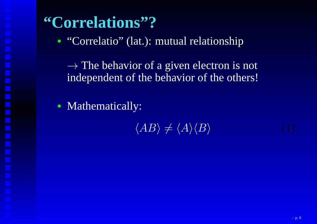
“Correlations”?• “Correlatio” (lat.): mutual relationship
→ The behavior of a given electron is notindependent of the behavior of the others!
– p. 4
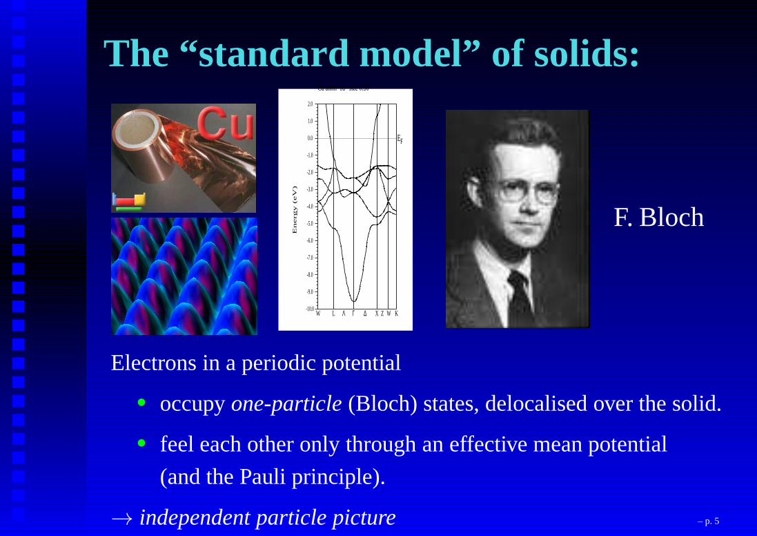
The “standard model” of solids:Cu atom 1d size 0.30
W L Λ Γ ∆ X Z W K
E F
En
erg
y (
eV
)
0.0
1.0
2.0
-1.0
-2.0
-3.0
-4.0
-5.0
-6.0
-7.0
-8.0
-9.0
-10.0
F. Bloch
Electrons in a periodic potential
• occupyone-particle(Bloch) states, delocalised over the solid.
• feel each other only through an effective mean potential
(and the Pauli principle).
→ independent particle picture – p. 5
“Correlations”?• “Correlatio” (lat.): mutual relationship
→ The behavior of a given electron is notindependent of the behavior of the others!
• Mathematically:
〈AB〉 6= 〈A〉〈B〉 (1)
– p. 6

“Correlations”?
50% have blue eyes50% have yellow eyes
– p. 7
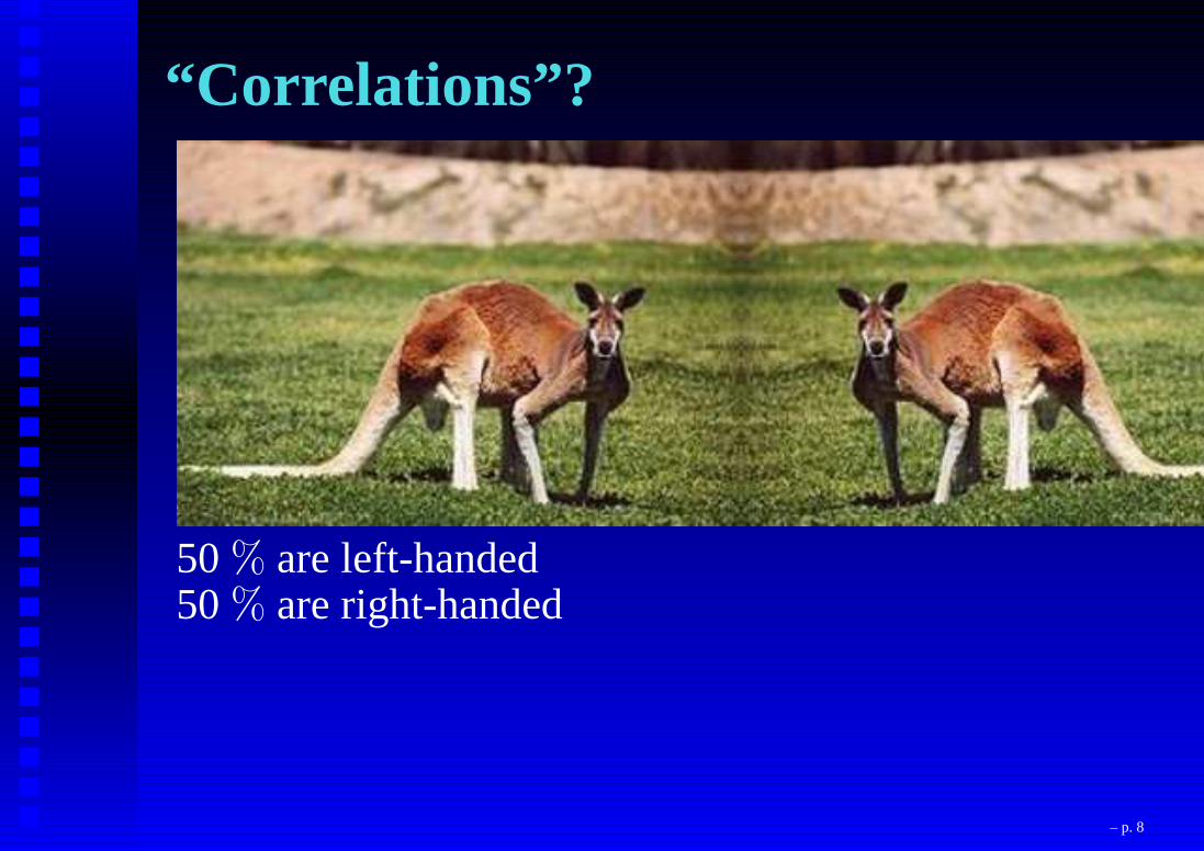
“Correlations”?
50% are left-handed50% are right-handed
– p. 8
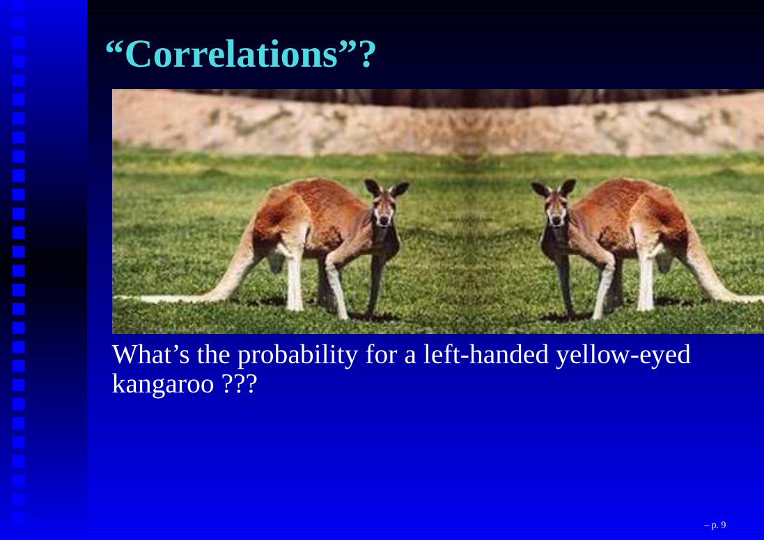
“Correlations”?
What’s the probability for a left-handed yellow-eyedkangaroo ???
– p. 9

“Correlations”?
probability for a left-handed yellow-eyed kangaroo= 1/2 · 1/2 = 1/4 only if the two properties areuncorrelatedOtherwise: anything can happen ....
– p. 10

“Correlations”?• “Correlatio” (lat.): mutual relationship
→ The behavior of a given electron is notindependent of the behavior of the others!
• Mathematically:
〈AB〉 6= 〈A〉〈B〉 (2)
For electrons (in a given atomic orbital):
〈n↑n↓〉 6= 〈n↑〉〈n↓〉
nσ = number operator for electrons with spinσ.
– p. 11

“Correlations”?Count electrons on a given atom in a given orbital:
nσ = counts electrons with spinσ
n↑n↓ counts “double-occupations”
〈n↑n↓〉 = 〈n↑〉〈n↓〉 only if the “second” electrondoes not care about the orbital being alreadyoccupied or not
– p. 12
Exercise (!):Does
〈n↑n↓〉 = 〈n↑〉〈n↓〉hold?
1. Hamiltonian:H0 = ǫ(n↑ + n↓)
2. Hamiltonian:H = ǫ(n↑ + n↓) + Un↑n↓
– p. 13

Correlations 〈n↑n↓〉 = 〈n↑〉〈n↓〉?
(1) Hamiltonian:H0 = ǫ(n↑ + n↓)Operatorsn↑ andn↓ have eigenvalues0 and1.
– p. 14
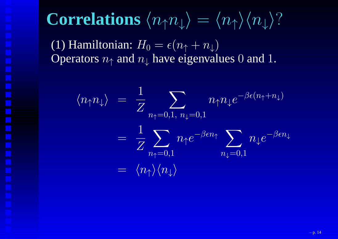
Correlations 〈n↑n↓〉 = 〈n↑〉〈n↓〉?
(1) Hamiltonian:H0 = ǫ(n↑ + n↓)Operatorsn↑ andn↓ have eigenvalues0 and1.
〈n↑n↓〉 =1
Z
∑
n↑=0,1, n↓=0,1
n↑n↓e−βǫ(n↑+n↓)
=1
Z
∑
n↑=0,1
n↑e−βǫn↑
∑
n↓=0,1
n↓e−βǫn↓
= 〈n↑〉〈n↓〉
– p. 14

Correlations 〈n↑n↓〉 = 〈n↑〉〈n↓〉?
(1) Hamiltonian:H0 = ǫ(n↑ + n↓)Operatorsn↑ andn↓ have eigenvalues0 and1.
〈n↑n↓〉 =1
Z
∑
n↑=0,1, n↓=0,1
n↑n↓e−βǫ(n↑+n↓)
=1
Z
∑
n↑=0,1
n↑e−βǫn↑
∑
n↓=0,1
n↓e−βǫn↓
= 〈n↑〉〈n↓〉
No correlations! (Hamiltonian separable)
– p. 14

Correlations 〈n↑n↓〉 = 〈n↑〉〈n↓〉?
(2) Hamiltonian:H = ǫ(n↑ + n↓) + Un↑n↓
Operatorsn↑ andn↓ have eigenvalues0 and1.
– p. 15

Correlations 〈n↑n↓〉 = 〈n↑〉〈n↓〉?
(2) Hamiltonian:H = ǫ(n↑ + n↓) + Un↑n↓
Operatorsn↑ andn↓ have eigenvalues0 and1.
〈n↑n↓〉 =1
Z
∑
n↑=0,1, n↓=0,1
n↑n↓e−βǫ(n↑+n↓)−βUn↑n↓
6= 〈n↑〉〈n↓〉
– p. 15

Correlations 〈n↑n↓〉 = 〈n↑〉〈n↓〉?
(2) Hamiltonian:H = ǫ(n↑ + n↓) + Un↑n↓
Operatorsn↑ andn↓ have eigenvalues0 and1.
〈n↑n↓〉 =1
Z
∑
n↑=0,1, n↓=0,1
n↑n↓e−βǫ(n↑+n↓)−βUn↑n↓
6= 〈n↑〉〈n↓〉
Correlations! (Hamiltonian not separable)
– p. 15
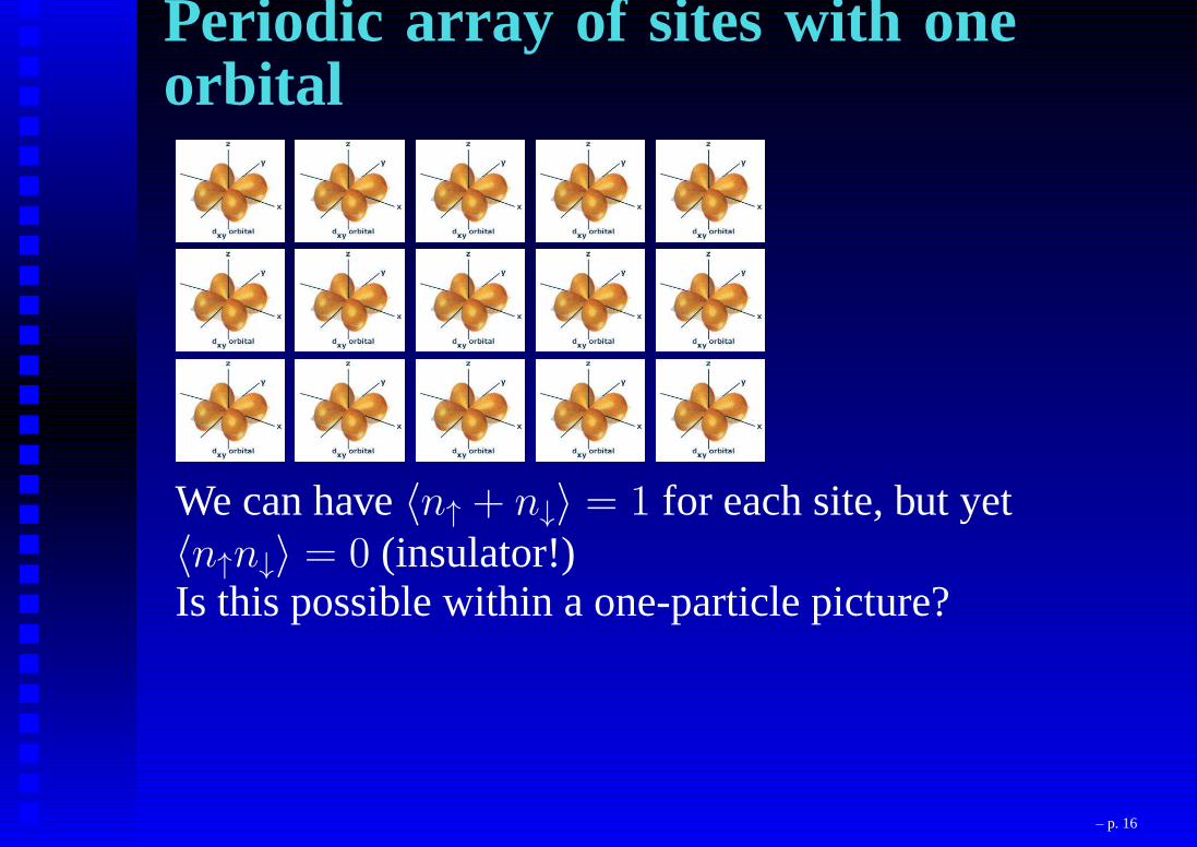
Periodic array of sites with oneorbital
We can have〈n↑ + n↓〉 = 1 for each site, but yet〈n↑n↓〉 = 0 (insulator!)Is this possible within a one-particle picture?
– p. 16
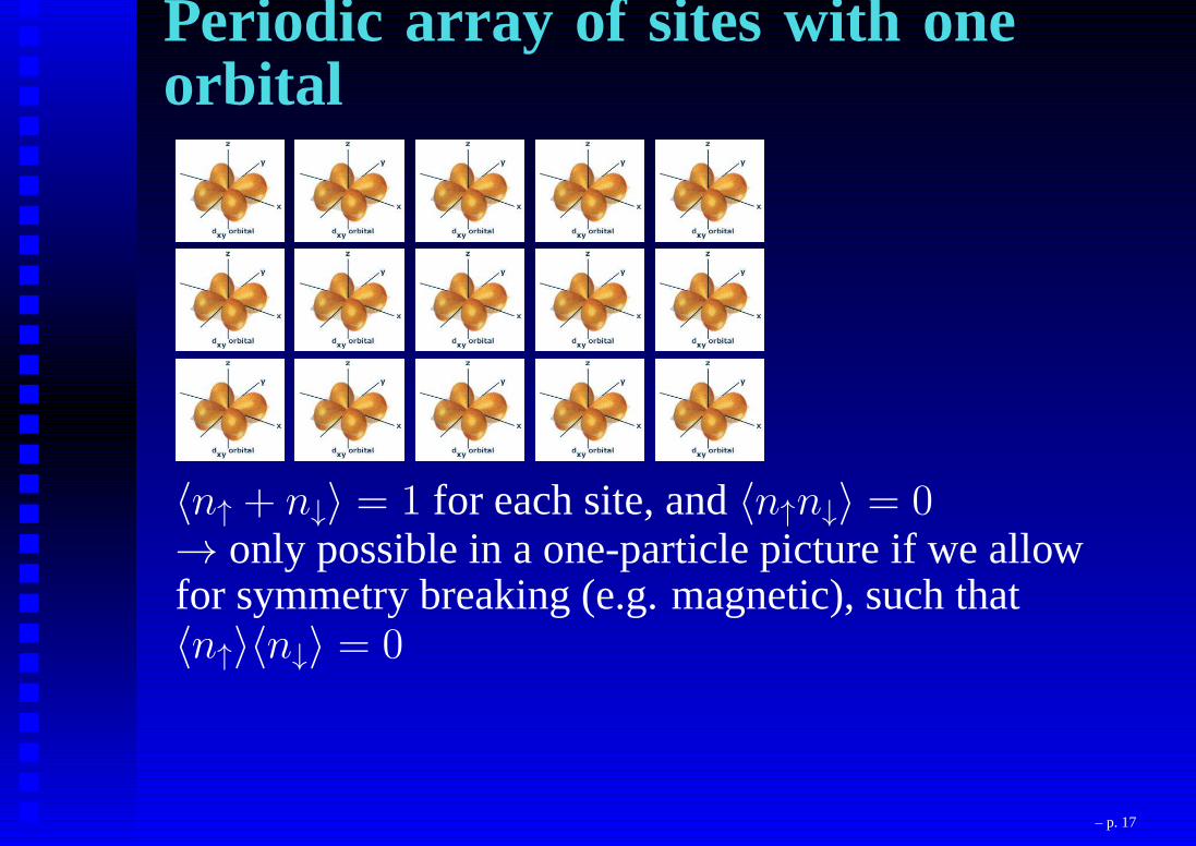
Periodic array of sites with oneorbital
〈n↑ + n↓〉 = 1 for each site, and〈n↑n↓〉 = 0→ only possible in a one-particle picture if we allowfor symmetry breaking (e.g. magnetic), such that〈n↑〉〈n↓〉 = 0
– p. 17

Mott’s ficticious H-solid:Hydrogen atoms with lattice spacing 1 m
H H H H H H H HH H H H H H H HH H H H H H H H (not to scale ...)H H H H H H H HH H H H H H H H
Metal or insulator?
– p. 18
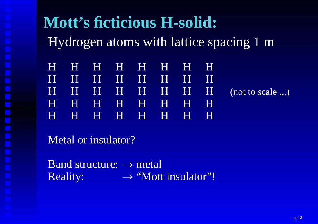
Mott’s ficticious H-solid:Hydrogen atoms with lattice spacing 1 m
H H H H H H H HH H H H H H H HH H H H H H H H (not to scale ...)H H H H H H H HH H H H H H H H
Metal or insulator?
Band structure:→ metalReality: → “Mott insulator”!
– p. 18

Mott’s ficticious H-solid:Hydrogen atoms with lattice spacing 1 m
H H H H H H H HH H H H H H H HH H H H H H H H (not to scale ...)H H H H H H H HH H H H H H H H
Metal or insulator?
Band structure:→ metalReality: → “Mott insulator”!
Coulomb repulsion dominates over kinetic energy!– p. 18
What are the energy scales?
– p. 19

What are the energy scales?Compare
Vm1m2m3m4≡ 〈φm1
φm2|
1
|r − r′||φm3
φm4〉
=
∫∫
drdr′φ∗m1(r)φm3
(r)1
|r − r′|φ∗m2(r′)φm4
(r′).
and kinetic energy
– p. 20

What are the energy scales?Compare
Vm1m2m3m4≡ 〈φm1
φm2|
1
|r − r′||φm3
φm4〉
=
∫∫
drdr′φ∗m1(r)φm3
(r)1
|r − r′|φ∗m2(r′)φm4
(r′).
and kinetic energy
For 3d Wannier function of typical transition metals:30 eV versus 3 eV !!
– p. 21

Why does band theory work atall?
– p. 22

Band structure ...... from photoemission – Example: Copper
– p. 23

Why does band theory work atall?Band structure relies onone-electronpictureBut: electrons interact !
Several answers ...:
•Pauli principleScreening reduce effects of interactions
Landau’s Fermi liquid theory: quasi-particles
– p. 24

Structure of SrVO33.1 Introduction 69
CaVO3 SrVO3
(a) (b)V
O
Sr
V
O
Ca
Figure 3.1: The crystal structure of (a) CaVO3 and (b) SrVO3 exhibiting various V-O-Vbond angles in the system.(= 180o) (see Fig. 3.1(b)) with cubic perovskite structure in SrVO3. Stoichiometric CaVO3and SrVO3 are both Pauli-paramagnetic metals [12-14]. Oxygen non-stoichiometry inCaVO3 leads to antiferromagnetic [15] or Curie-Weiss paramagnetic [16] behavior withno long range magnetic order down to 4 K. A solid solution of CaVO3 and SrVO3 can beformed over the entire composition range (0 x 1) with the formula Ca1xSrxVO3.Ca and Sr being homovalent (2+) in the solid solution, there is no change in the chargecarrier concentration with composition (x) and it is always one electron per V-ion acrossthe series. On the other hand, the dierent V-O-V bond angle results in dierent V-O-V hopping interaction strength, t. Thus, the eective correlation strength as measuredby U=W where W (/ t) denotes the bare bandwidth of the system, can be continuouslytuned by changing x, with CaVO3 being a more correlated metal with a larger U=W valuethan SrVO3 [11]. Thus, these compounds represent a well-suited experimental realizationof a continuous tuning of U=W and consequently, provide a good testing ground for thepredictions of the Hubbard model.With this in view, the electronic structure of Ca1xSrxVO3 was probed for severalvalues of x using photoelectron spectroscopy [11]. The experimental results are shown tobe incompatible with the existing theoretical results described in terms of the Hubbard
SrVO3: a cubic perovskite
– p. 25

The “standard model” (contd.)Landau theory of quasiparticles:→ one-particle picture as a low-energy theorywith renormalized parameters
Inte
nsity
(ar
b. u
nits
)
-2.5 -2.0 -1.5 -1.0 -0.5 0 -2.5 -2.0 -1.5 -1.0 -0.5 0
-0.6
-0.4
-0.2
0
0.2
0.4
0.6
k y (π
/a)
Energy relative to EF (eV)
(c) SrVO3 hν=90 eV (d) CaVO3 hν=80 eV
(a) (b)SrVO3 atom 0 size 0.20
R Λ Γ ∆ X Z M Σ Γ
E F
Ene
rgy
(eV
)
0.0
1.0
2.0
-1.0
-2.0
– p. 26
Why does band theory work atall?Band structure relies onone-electronpictureBut: electrons interact !
Several answers ...:
•Pauli principleScreening reduce effects of interactions
Landau’s Fermi liquid theory: quasi-particles
– p. 27

Why does band theory work atall?Band structure relies onone-electronpictureBut: electrons interact !
Several answers ...:
•Pauli principleScreening reduce effects of interactions
Landau’s Fermi liquid theory: quasi-particles
• It does not always work ....
– p. 28
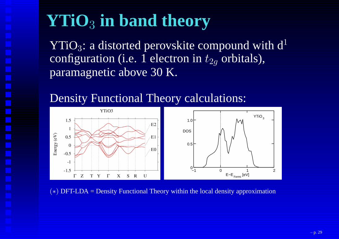
YTiO 3 in band theoryYTiO3: a distorted perovskite compound with d1
configuration (i.e. 1 electron int2g orbitals),paramagnetic above 30 K.
Density Functional Theory calculations:
0
0.5
1.0
−1 0 1 2E−E
Fermi[eV]
DOS
YTiO3
(∗) DFT-LDA = Density Functional Theory within the local density approximation
– p. 29

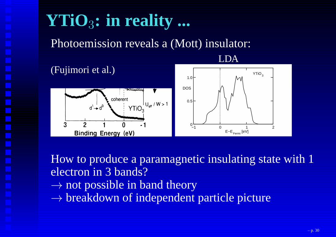
YTiO 3: in reality ...Photoemission reveals a (Mott) insulator:
(Fujimori et al.)LDA
0
0.5
1.0
−1 0 1 2E−E
Fermi[eV]
DOS
YTiO3
– p. 30
YTiO 3: in reality ...Photoemission reveals a (Mott) insulator:
(Fujimori et al.)LDA
0
0.5
1.0
−1 0 1 2E−E
Fermi[eV]
DOS
YTiO3
How to produce a paramagnetic insulating state with 1electron in 3 bands?→ not possible in band theory→ breakdown of independent particle picture
– p. 30

Can we understand correlated electronic behavior?
How to (quantitatively?) describe correlatedmaterials?
– p. 31
Further outline• Correlated Materials – some (more) examples• Modelling correlated electron: Hubbard model• The Mott metal-insulator transition• Dynamical mean field theory (DMFT)• Density Functional Theory (DFT) within the
Local Density Approximation (LDA)• Dynamical mean field theory within electronic
structure calculations (“LDA+DMFT”)• Current questions in the field: what about U? ...• Beyond LDA+DMFT? – Functional approaches• Conclusions
– p. 32
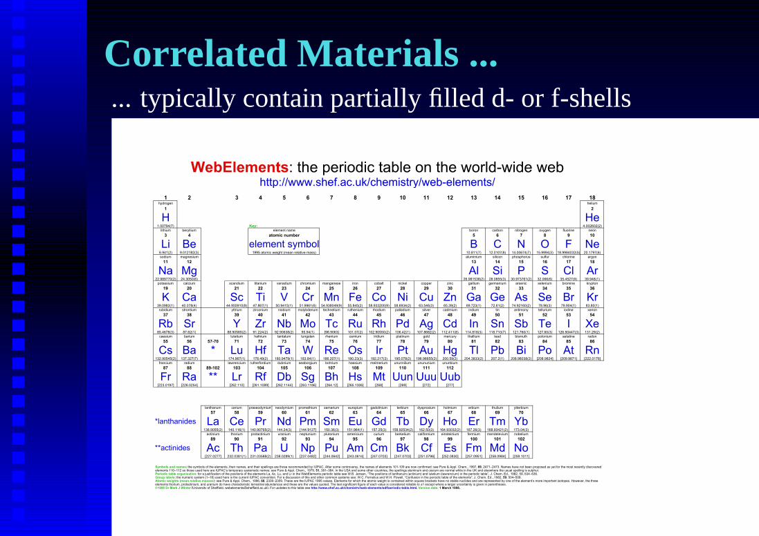
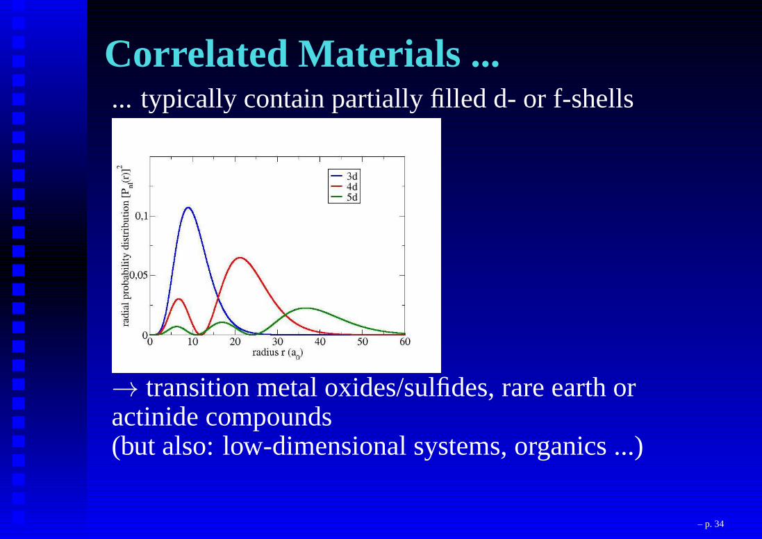
Correlated Materials ...... typically contain partially filled d- or f-shells
1 2 3 4 5 6 7 8 9 10 11 12 13 14 15 16 17 18hydrogen helium
1 2
H He1.00794(7) Key: 4.002602(2)
lithium beryllium element name boron carbon nitrogen oxygen fluorine neon
3 4 atomic number 5 6 7 8 9 10
Li Be element symbol B C N O F Ne6.941(2) 9.012182(3) 1995 atomic weight (mean relative mass) 10.811(7) 12.0107(8) 14.00674(7) 15.9994(3) 18.9984032(5) 20.1797(6)
sodium magnesium aluminium silicon phosphorus sulfur chlorine argon
11 12 13 14 15 16 17 18
Na Mg Al Si P S Cl Ar22.989770(2) 24.3050(6) 26.981538(2) 28.0855(3) 30.973761(2) 32.066(6) 35.4527(9) 39.948(1)
potassium calcium scandium titanium vanadium chromium manganese iron cobalt nickel copper zinc gallium germanium arsenic selenium bromine krypton
19 20 21 22 23 24 25 26 27 28 29 30 31 32 33 34 35 36
K Ca Sc Ti V Cr Mn Fe Co Ni Cu Zn Ga Ge As Se Br Kr39.0983(1) 40.078(4) 44.955910(8) 47.867(1) 50.9415(1) 51.9961(6) 54.938049(9) 55.845(2) 58.933200(9) 58.6934(2) 63.546(3) 65.39(2) 69.723(1) 72.61(2) 74.92160(2) 78.96(3) 79.904(1) 83.80(1)
rubidium strontium yttrium zirconium niobium molybdenum technetium ruthenium rhodium palladium silver cadmium indium tin antimony tellurium iodine xenon
37 38 39 40 41 42 43 44 45 46 47 48 49 50 51 52 53 54
Rb Sr Y Zr Nb Mo Tc Ru Rh Pd Ag Cd In Sn Sb Te I Xe85.4678(3) 87.62(1) 88.90585(2) 91.224(2) 92.90638(2) 95.94(1) [98.9063] 101.07(2) 102.90550(2) 106.42(1) 107.8682(2) 112.411(8) 114.818(3) 118.710(7) 121.760(1) 127.60(3) 126.90447(3) 131.29(2)
caesium barium lutetium hafnium tantalum tungsten rhenium osmium iridium platinum gold mercury thallium lead bismuth polonium astatine radon
55 56 57-70 71 72 73 74 75 76 77 78 79 80 81 82 83 84 85 86
Cs Ba * Lu Hf Ta W Re Os Ir Pt Au Hg Tl Pb Bi Po At Rn132.90545(2) 137.327(7) 174.967(1) 178.49(2) 180.9479(1) 183.84(1) 186.207(1) 190.23(3) 192.217(3) 195.078(2) 196.96655(2) 200.59(2) 204.3833(2) 207.2(1) 208.98038(2) [208.9824] [209.9871] [222.0176]
francium radium lawrencium rutherfordium dubnium seaborgium bohrium hassium meitnerium ununnilium unununium ununbium
87 88 89-102 103 104 105 106 107 108 109 110 111 112
Fr Ra ** Lr Rf Db Sg Bh Hs Mt Uun Uuu Uub[223.0197] [226.0254] [262.110] [261.1089] [262.1144] [263.1186] [264.12] [265.1306] [268] [269] [272] [277]
lanthanum cerium praseodymium neodymium promethium samarium europium gadolinium terbium dysprosium holmium erbium thulium ytterbium
57 58 59 60 61 62 63 64 65 66 67 68 69 70
*lanthanides La Ce Pr Nd Pm Sm Eu Gd Tb Dy Ho Er Tm Yb138.9055(2) 140.116(1) 140.90765(2) 144.24(3) [144.9127] 150.36(3) 151.964(1) 157.25(3) 158.92534(2) 162.50(3) 164.93032(2) 167.26(3) 168.93421(2) 173.04(3)
actinium thorium protactinium uranium neptunium plutonium americium curium berkelium californium einsteinium fermium mendelevium nobelium
89 90 91 92 93 94 95 96 97 98 99 100 101 102
**actinides Ac Th Pa U Np Pu Am Cm Bk Cf Es Fm Md No[227.0277] 232.0381(1) 231.03588(2) 238.0289(1) [237.0482] [244.0642] [243.0614] [247.0703] [247.0703] [251.0796] [252.0830] [257.0951] [258.0984] [259.1011]
WebElements: the periodic table on the world-wide webhttp://www.shef.ac.uk/chemistry/web-elements/
Symbols and names: the symbols of the elements, their names, and their spellings are those recommended by IUPAC. After some controversy, the names of elements 101-109 are now confirmed: see Pure & Appl. Chem., 1997, 69, 2471Ð2473. Names have not been proposed as yet for the most recently discovered elements 110Ð112 so those used here are IUPACÕs temporary systematic names: see Pure & Appl. Chem., 1979, 51, 381Ð384. In the USA and some other countries, the spellings aluminum and cesium are normal while in the UK and elsewhere the usual spelling is sulphur. Periodic table organisation: for a justification of the positions of the elements La, Ac, Lu, and Lr in the WebElements periodic table see W.B. Jensen, ÒThe positions of lanthanum (actinium) and lutetium (lawrencium) in the periodic tableÓ, J. Chem. Ed., 1982, 59, 634Ð636. Group labels: the numeric system (1Ð18) used here is the current IUPAC convention. For a discussion of this and other common systems see: W.C. Fernelius and W.H. Powell, ÒConfusion in the periodic table of the elementsÓ, J. Chem. Ed., 1982, 59, 504Ð508.Atomic weights (mean relative masses): see Pure & Appl. Chem., 1996, 68, 2339Ð2359. These are the IUPAC 1995 values. Elements for which the atomic weight is contained within square brackets have no stable nuclides and are represented by one of the elementÕs more important isotopes. However, the three elements thorium, protactinium, and uranium do have characteristic terrestrial abundances and these are the values quoted. The last significant figure of each value is considered reliable to ±1 except where a larger uncertainty is given in parentheses.©1998 Dr Mark J Winter [University of Sheffield, [email protected]]. For updates to this table see http://www.shef.ac.uk/chemistry/web-elements/pdf/periodic-table.html. Version date: 1 March 1998.
– p. 33
Correlated Materials ...... typically contain partially filled d- or f-shells
→ transition metal oxides/sulfides, rare earth oractinide compounds(but also: low-dimensional systems, organics ...)
– p. 34
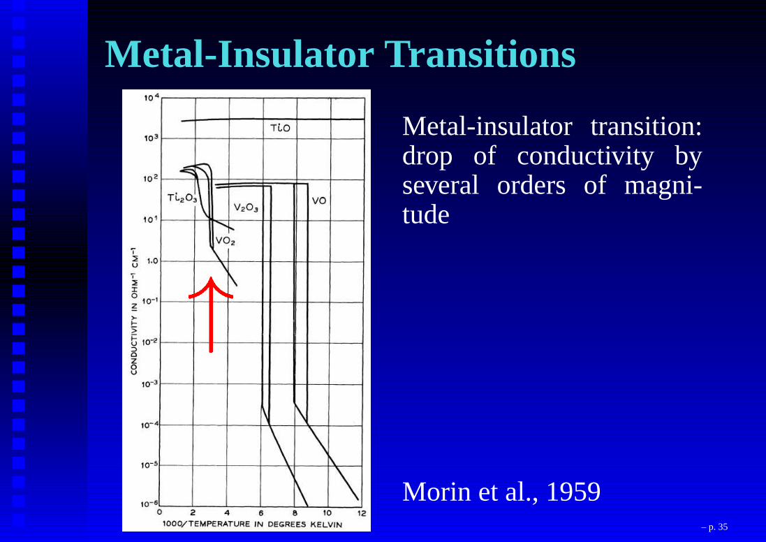
Metal-Insulator Transitions
Metal-insulator transition:drop of conductivity byseveral orders of magni-tude
Morin et al., 1959!
– p. 35

SrVO3 : a correlated metalSrVO3 within DFT-LDA
0
0.1
0.2
0.3
0.4
0.5
0.6
-1.5 -1 -0.5 0 0.5 1 1.5
Ni,i
(E)
E (eV)
SrVO3
0
0.1
0.2
0.3
0.4
0.5
0.6
-1.5 -1 -0.5 0 0.5 1 1.5
Ni,i
(E)
E (eV)
SrVO3
0
0.1
0.2
0.3
0.4
0.5
0.6
-1.5 -1 -0.5 0 0.5 1 1.5
Ni,i
(E)
E (eV)
SrVO3
-0.2
-0.1
0
0.1
0.2
-1 0 1
E (eV)
Ni,j(E)
-0.2
-0.1
0
0.1
0.2
-1 0 1
E (eV)
Ni,j(E)
-0.2
-0.1
0
0.1
0.2
-1 0 1
E (eV)
Ni,j(E)
Photoemission
Inte
nsi
ty (
arb
. units
)
2.0 1.0 0.0Binding Energy (eV)
Sr0.5Ca0.5VO3
SrVO3 (x = 0)
CaVO3 (x = 1)
hν = 900 eV hν = 275 eV hν = 40.8 eV hν = 21.2 eV
(Sekiyama et al. 2003)
– p. 36

Iron pnictides
LaFePO: photoemission versus band structure(Lu et al., 2008)
– p. 37
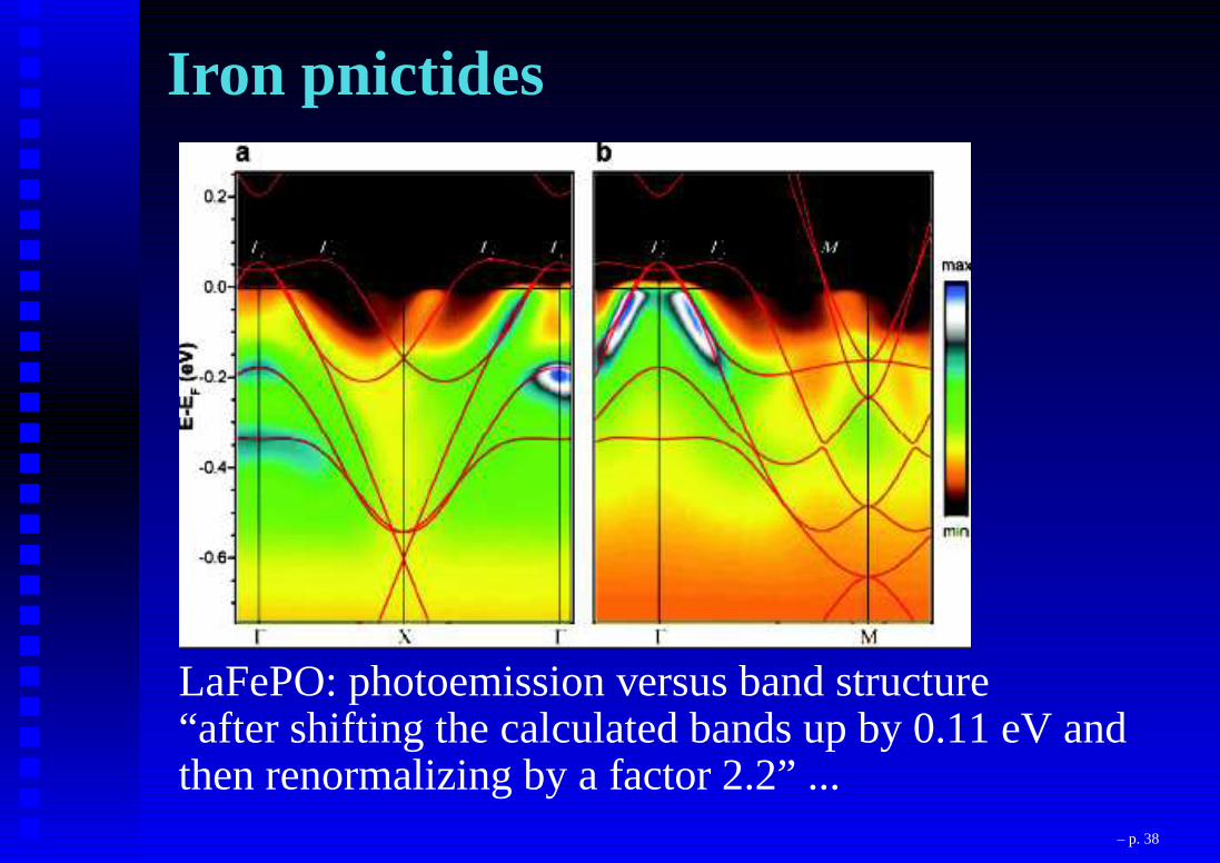
Iron pnictides
LaFePO: photoemission versus band structure“after shifting the calculated bands up by 0.11 eV andthen renormalizing by a factor 2.2” ...
– p. 38
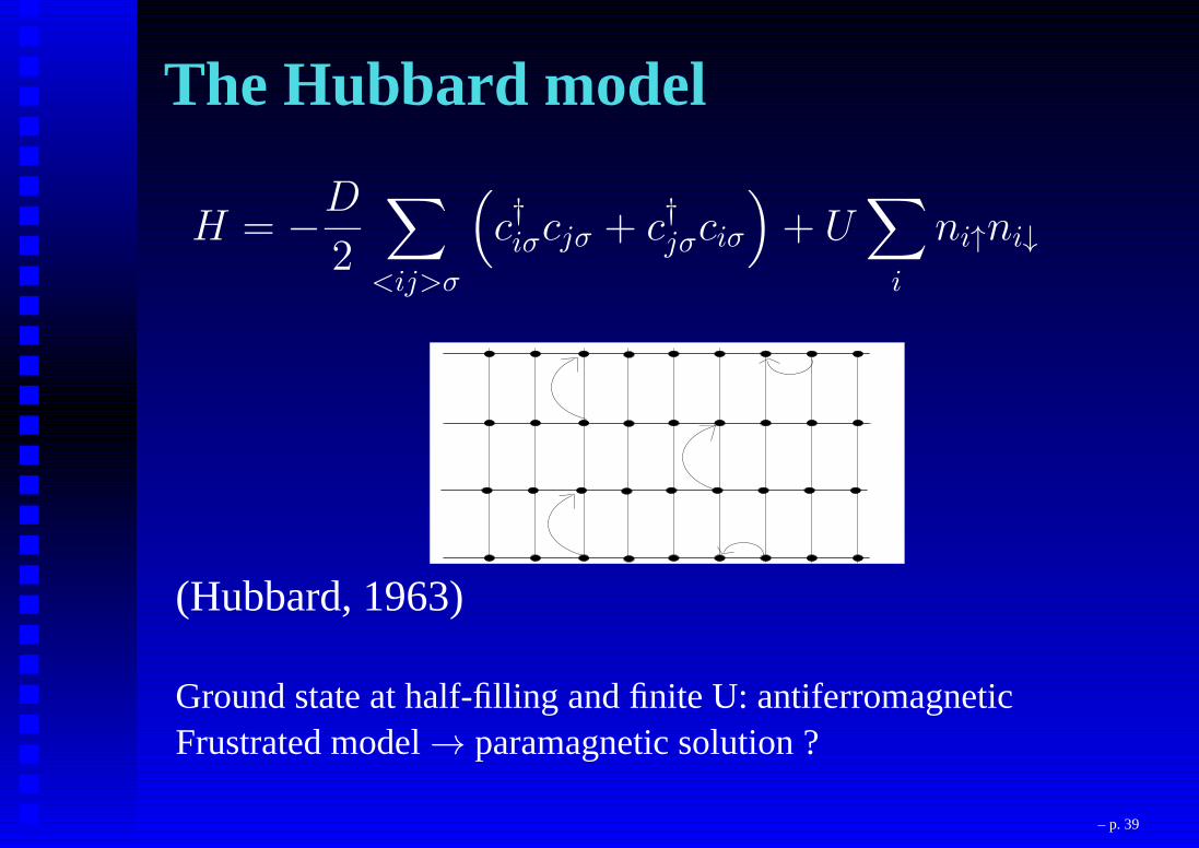
The Hubbard model
H = −D
2
∑
<ij>σ
(
c†iσcjσ + c†jσciσ
)
+ U∑
i
ni↑ni↓
(Hubbard, 1963)
Ground state at half-filling and finite U: antiferromagneticFrustrated model→ paramagnetic solution ?
– p. 39

Spectra for one atomElectron removal and addition spectra
0
0.2
0.4
0.6
0.8
1
-1.5 -1 -0.5 0 0.5 1 1.5
’ell.dat’
E = ǫ E = ǫ+ U
U=Coulomb interaction between two 1s electrons
– p. 40

Atomic limit: D=0
H = U∑
i
ni↑ni↓
→ atomic eigenstates, localized inreal space
Spectral function = discrete peaks separated by U
0
0.2
0.4
0.6
0.8
1
-1.5 -1 -0.5 0 0.5 1 1.5
’ell.dat’
– p. 41
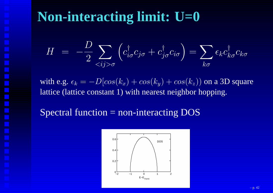
Non-interacting limit: U=0
H = −D
2
∑
<ij>σ
(
c†iσcjσ + c†jσciσ
)
=∑
kσ
ǫkc†kσckσ
with e.g.ǫk = −D[cos(kx) + cos(ky) + cos(kz)) on a 3D squarelattice (lattice constant 1) with nearest neighbor hopping.
Spectral function = non-interacting DOS
0
0.2
0.4
0.6
−2 −1 0 1 2E−E
Fermi
DOS
– p. 42

“Atomic” and “band-like” spectra
0
0.1
0.2
0.3
0.4
0.5
−10 −5 0 5 10E−E
Fermi
U
0
0.2
0.4
0.6
−2 −1 0 1 2E−E
Fermi
DOS
“Spectral function” ρ(ω) probes possibility ofadding/removing an electron at energyω.
In non-interacting case:ρ(ω)= DOS.In general case: relaxation effects!In “atomic limit”: probe local Coulomb interaction
– p. 43
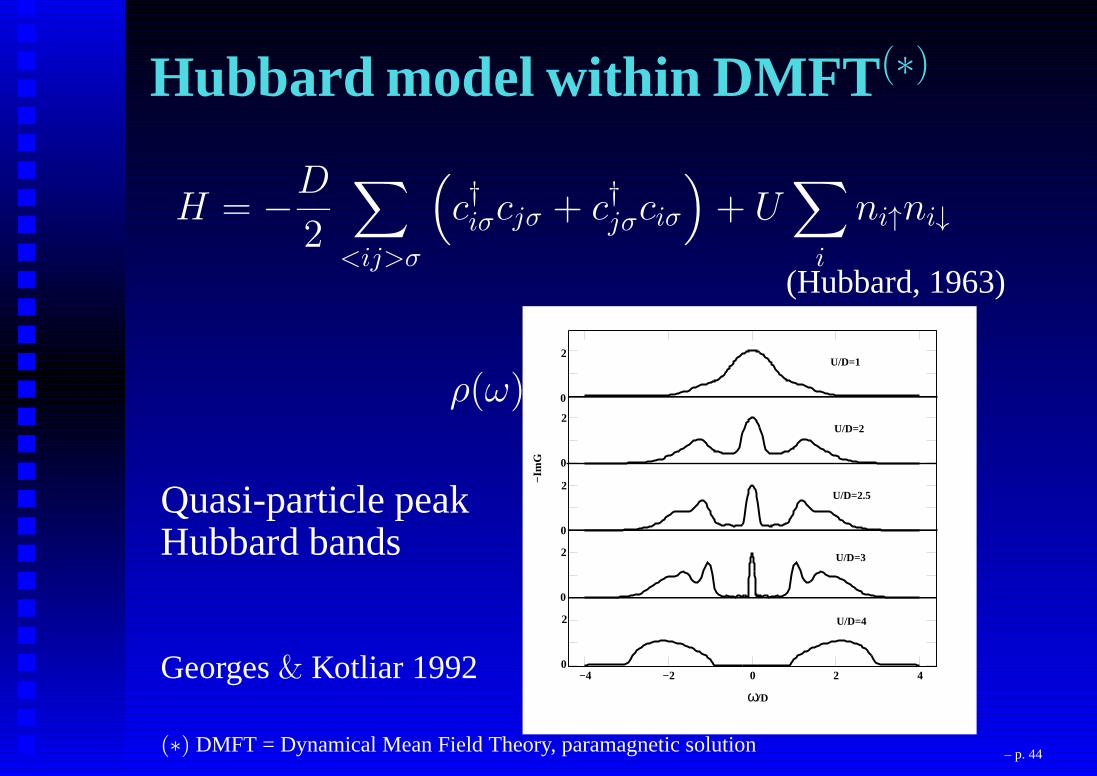
Hubbard model within DMFT (∗)
H = −D
2
∑
<ij>σ
(
c†iσcjσ + c†jσciσ
)
+ U∑
i
ni↑ni↓
(Hubbard, 1963)
2
0
2
0
2
0
2
0
2
0
−Im
G
ω−4 −2 0 2 4
U/D=1
U/D=2
U/D=2.5
U/D=3
U/D=4
/D
Quasi-particle peakHubbard bands
ρ(ω)
Georges& Kotliar 1992
(∗) DMFT = Dynamical Mean Field Theory, paramagnetic solution – p. 44
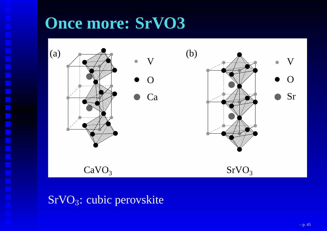
Once more: SrVO33.1 Introduction 69
CaVO3 SrVO3
(a) (b)V
O
Sr
V
O
Ca
Figure 3.1: The crystal structure of (a) CaVO3 and (b) SrVO3 exhibiting various V-O-Vbond angles in the system.(= 180o) (see Fig. 3.1(b)) with cubic perovskite structure in SrVO3. Stoichiometric CaVO3and SrVO3 are both Pauli-paramagnetic metals [12-14]. Oxygen non-stoichiometry inCaVO3 leads to antiferromagnetic [15] or Curie-Weiss paramagnetic [16] behavior withno long range magnetic order down to 4 K. A solid solution of CaVO3 and SrVO3 can beformed over the entire composition range (0 x 1) with the formula Ca1xSrxVO3.Ca and Sr being homovalent (2+) in the solid solution, there is no change in the chargecarrier concentration with composition (x) and it is always one electron per V-ion acrossthe series. On the other hand, the dierent V-O-V bond angle results in dierent V-O-V hopping interaction strength, t. Thus, the eective correlation strength as measuredby U=W where W (/ t) denotes the bare bandwidth of the system, can be continuouslytuned by changing x, with CaVO3 being a more correlated metal with a larger U=W valuethan SrVO3 [11]. Thus, these compounds represent a well-suited experimental realizationof a continuous tuning of U=W and consequently, provide a good testing ground for thepredictions of the Hubbard model.With this in view, the electronic structure of Ca1xSrxVO3 was probed for severalvalues of x using photoelectron spectroscopy [11]. The experimental results are shown tobe incompatible with the existing theoretical results described in terms of the Hubbard
SrVO3: cubic perovskite
– p. 45

Spectra of perovskitesPhotoemission
Inte
nsi
ty (
arb
. units
)
2.0 1.0 0.0Binding Energy (eV)
Sr0.5Ca0.5VO3
SrVO3 (x = 0)
CaVO3 (x = 1)
hν = 900 eV hν = 275 eV hν = 40.8 eV hν = 21.2 eV
(Sekiyama et al. 2003)
– p. 46

Spectra of perovskitesPhotoemission
Inte
nsi
ty (
arb
. units
)
2.0 1.0 0.0Binding Energy (eV)
Sr0.5Ca0.5VO3
SrVO3 (x = 0)
CaVO3 (x = 1)
hν = 900 eV hν = 275 eV hν = 40.8 eV hν = 21.2 eV
2
0
2
0
2
0
2
0
2
0
−Im
G
ω−4 −2 0 2 4
U/D=1
U/D=2
U/D=2.5
U/D=3
U/D=4
/D
(Sekiyama et al. 2003)
– p. 47
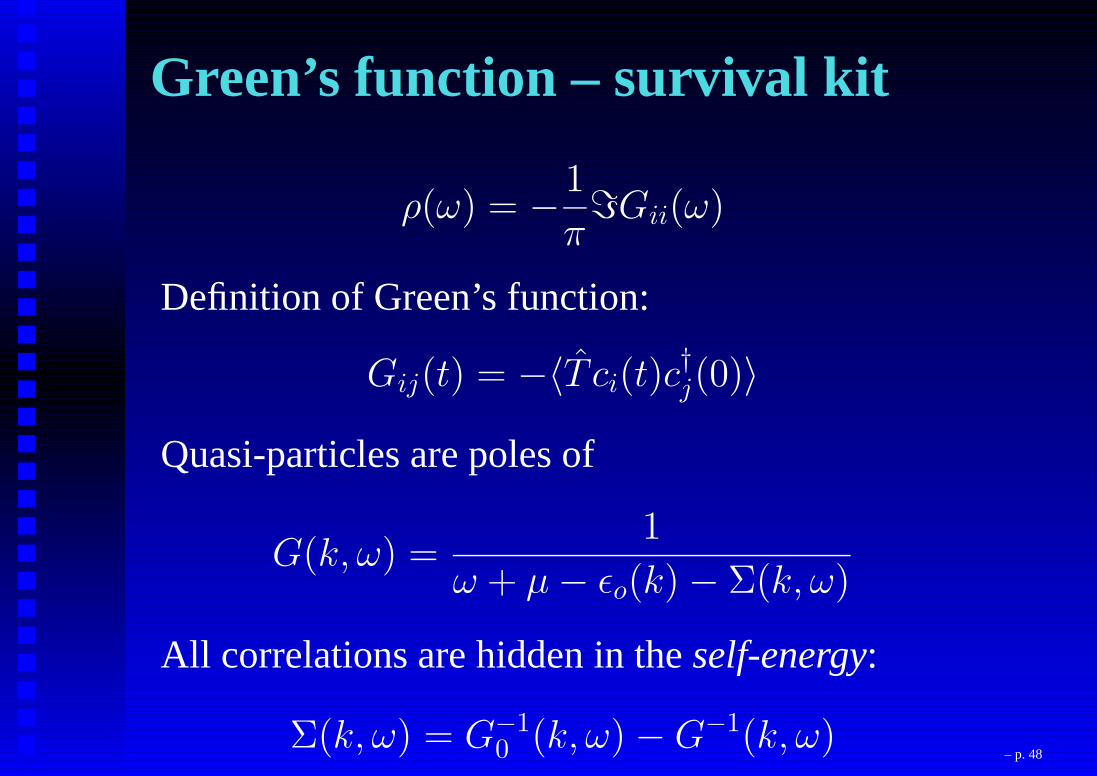
Green’s function – survival kit
ρ(ω) = −1
πℑGii(ω)
Definition of Green’s function:
Gij(t) = −〈T ci(t)c†j(0)〉
Quasi-particles are poles of
G(k, ω) =1
ω + µ− ǫo(k)− Σ(k, ω)
All correlations are hidden in theself-energy:
Σ(k, ω) = G−10 (k, ω)−G−1(k, ω)
– p. 48

Hubbard model within DMFT (∗)
H = −D
2
∑
<ij>σ
(
c†iσcjσ + c†jσciσ
)
+ U∑
i
ni↑ni↓
(Hubbard, 1963)
2
0
2
0
2
0
2
0
2
0
−Im
G
ω−4 −2 0 2 4
U/D=1
U/D=2
U/D=2.5
U/D=3
U/D=4
/D
Quasi-particle peakHubbard bands
ρ(ω)
Georges& Kotliar 1992
(∗) DMFT = Dynamical Mean Field Theory, paramagnetic solution – p. 49

Spectral functionQuasi-particle lifetime (∼ 1/Σ′′(ω = 0)) vanishes!→ Opening of a gap at the Fermi levelω = 0
A(k, ω) = ImG(k, ω)
= Im1
ω + µ− ǫo(k)− Σ(k, ω)
= −1
π
Σ′′(k, ω)
(ω + µ− ǫo(k)− Σ′(k, ω))2 + Σ′′(k, ω)2
Here: self-energy purely local. Then:
A(k, ω) = −1
π
Σ′′(ω)
(ω + µ− ǫo(k)Σ′(ω))2 + Σ′′(ω)2
→ Σ′′(ω) = inverse lifetime of excitation– p. 50

In a Fermi liquid:(local self-energy, for simplicity ...):
ImΣ(ω) = −Γω2 +O(ω3)
ReΣ(ω) = ReΣ(0) + (1− Z−1)ω +O(ω2)
A(k, ω) =Z2
π
−ℑΣ(ω)
(ω − Zǫ0(k))2 + (−ZℑΣ(ω))2
+Ainkoh
For small ImΣ (i.e. well-defined quasi-particles):Lorentzian of width ZImΣ,poles at renormalized quasi-particle bands Zǫ0(k),weight Z (instead of 1 in non-interacting case)
– p. 51

Hubbard model within DMFT (∗)
H = −D
2
∑
<ij>σ
(
c†iσcjσ + c†jσciσ
)
+ U∑
i
ni↑ni↓
(Hubbard, 1963)
2
0
2
0
2
0
2
0
2
0
−Im
G
ω−4 −2 0 2 4
U/D=1
U/D=2
U/D=2.5
U/D=3
U/D=4
/D
Quasi-particle peakHubbard bands
ρ(ω)
Georges& Kotliar 1992
(∗) DMFT = Dynamical Mean Field Theory, paramagnetic solution– p. 52
What’s ...... Dynamical Mean Field Theory (DMFT)?
– p. 53

What’s a mean field theory?
– p. 54
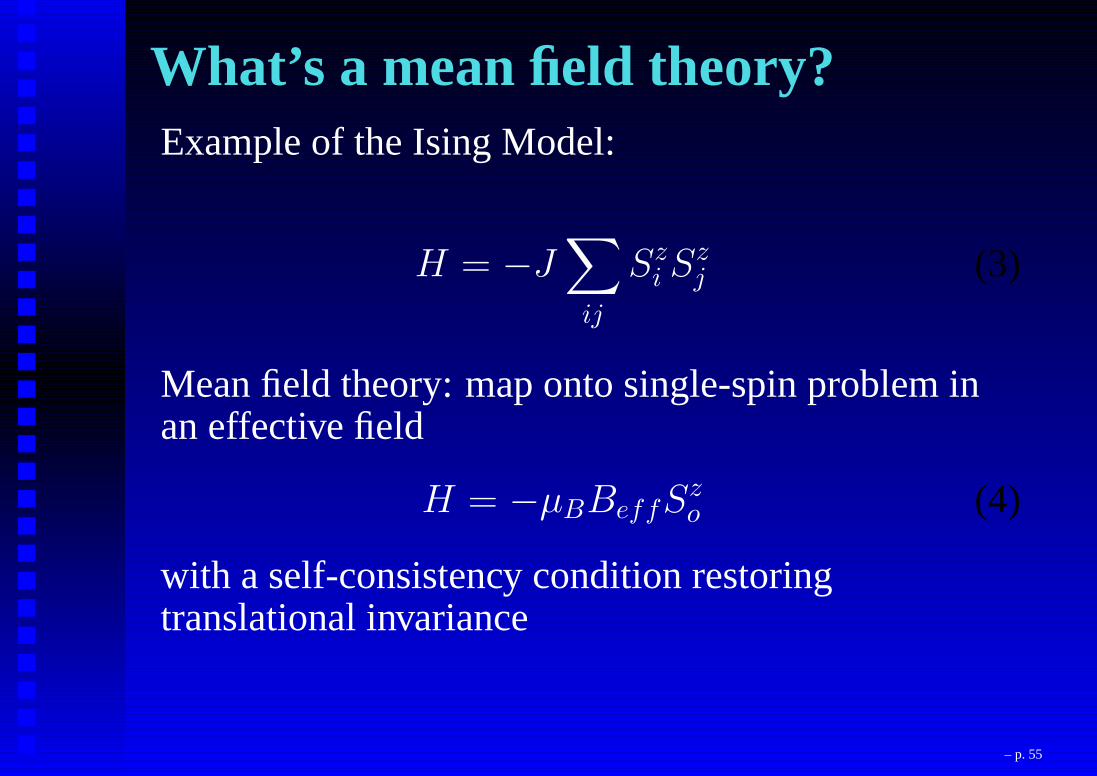
What’s a mean field theory?Example of the Ising Model:
H = −J∑
ij
Szi S
zj (3)
Mean field theory: map onto single-spin problem inan effective field
H = −µBBeffSzo (4)
with a self-consistency condition restoringtranslational invariance
– p. 55

What’s a mean field theory?Two ingredients:1. Reference system: single site (or cluster of sites) inan effective mean field
2. Self-consistency condition relating the effectiveproblem to the original one
– p. 56
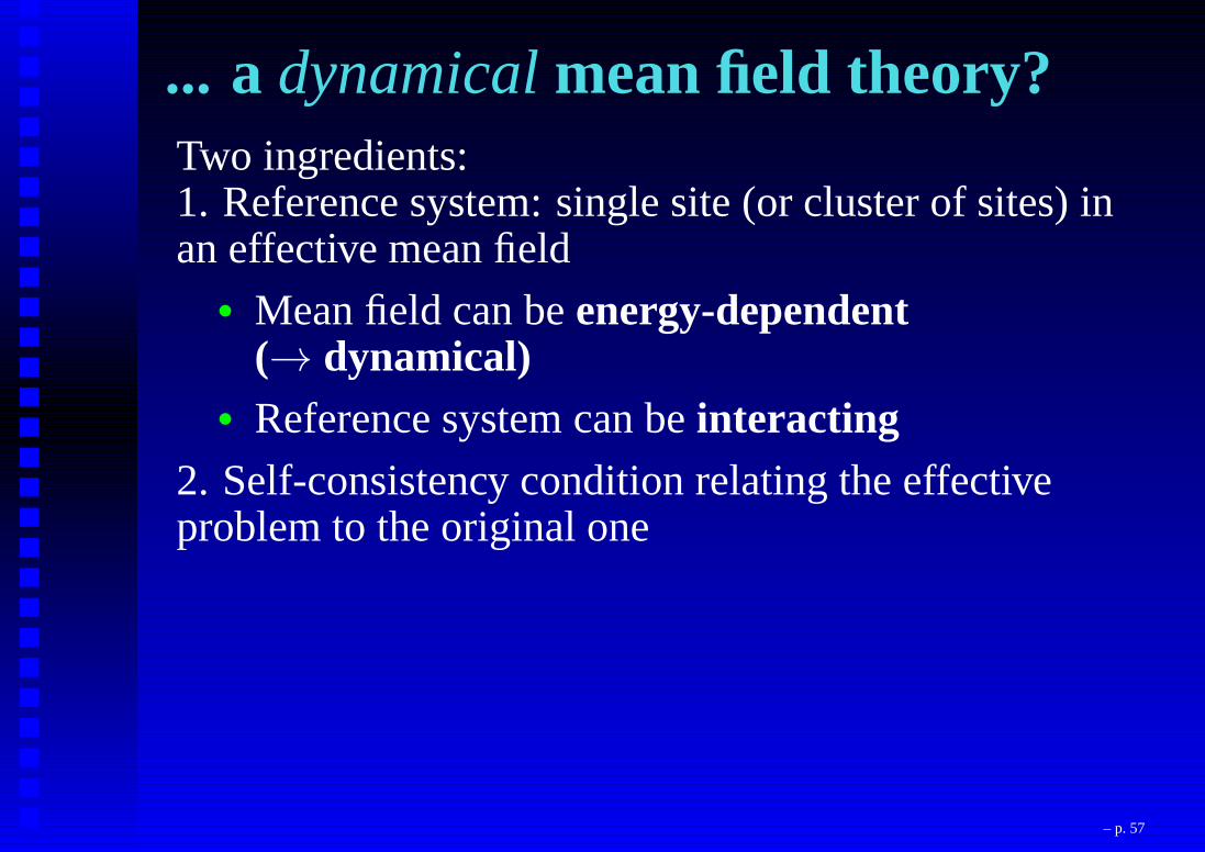
... adynamicalmean field theory?Two ingredients:1. Reference system: single site (or cluster of sites) inan effective mean field
• Mean field can beenergy-dependent(→ dynamical)
• Reference system can beinteracting2. Self-consistency condition relating the effectiveproblem to the original one
– p. 57
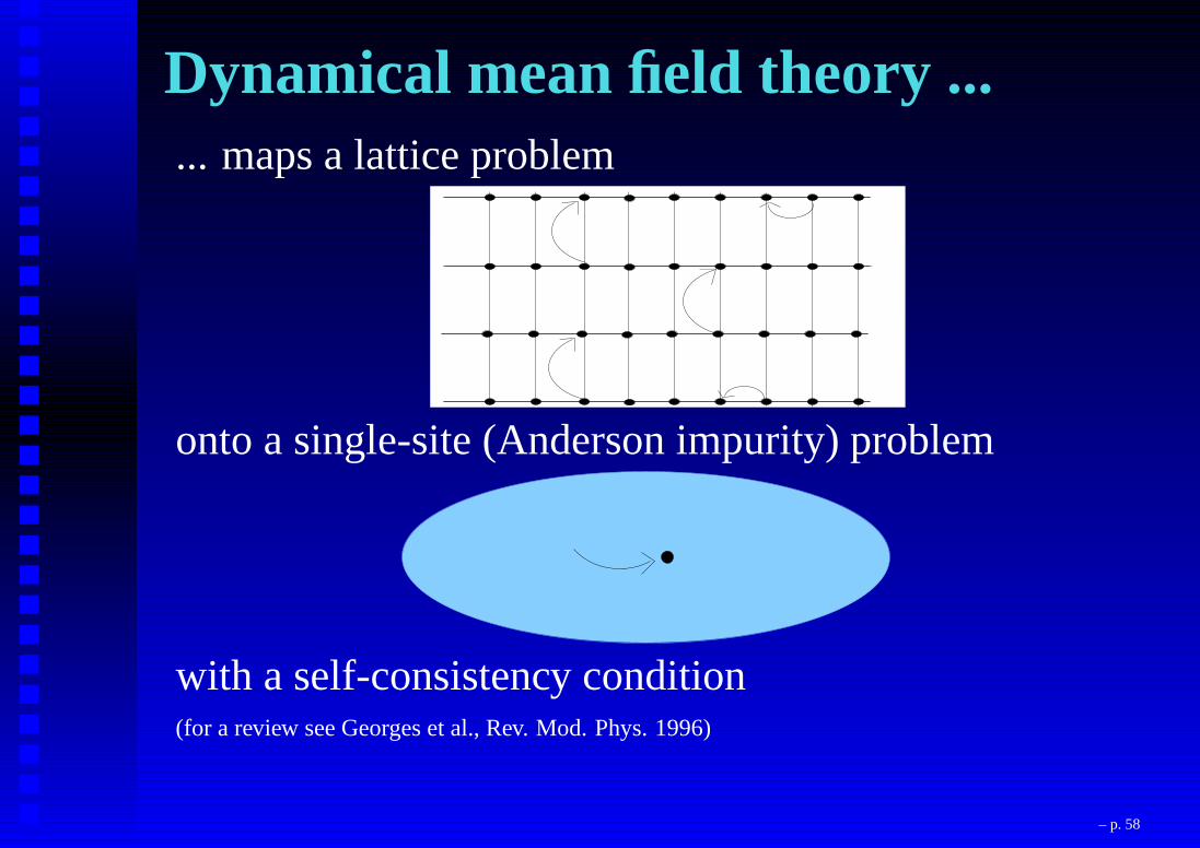
Dynamical mean field theory ...... maps a lattice problem
onto a single-site (Anderson impurity) problem
with a self-consistency condition(for a review see Georges et al., Rev. Mod. Phys. 1996)
– p. 58
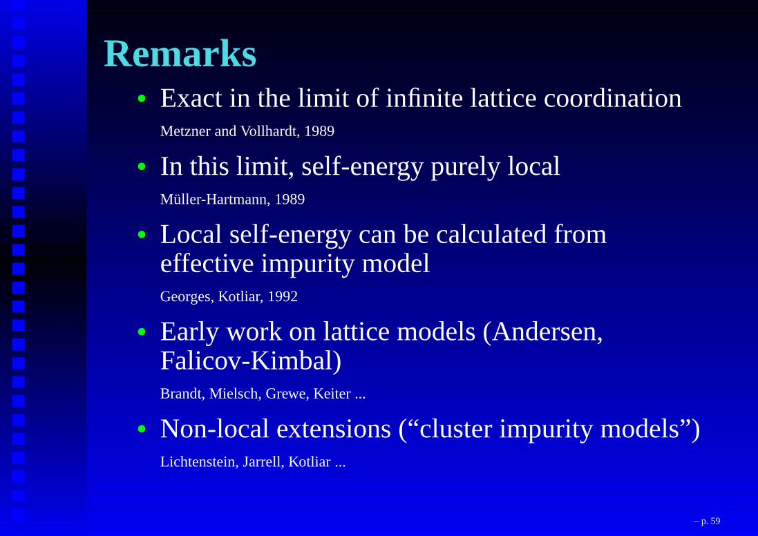
Remarks• Exact in the limit of infinite lattice coordination
Metzner and Vollhardt, 1989
• In this limit, self-energy purely localMüller-Hartmann, 1989
• Local self-energy can be calculated fromeffective impurity modelGeorges, Kotliar, 1992
• Early work on lattice models (Andersen,Falicov-Kimbal)Brandt, Mielsch, Grewe, Keiter ...
• Non-local extensions (“cluster impurity models”)Lichtenstein, Jarrell, Kotliar ...
– p. 59

Dynamical mean field theory ...... maps a lattice problem
onto a single-site (Anderson impurity) problem
with a self-consistency condition(see e.g. Georges et al., Rev. Mod. Phys. 1996)
– p. 60
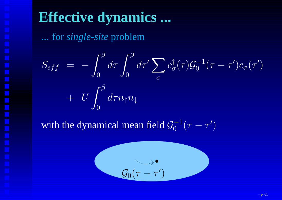
Effective dynamics ...... for single-siteproblem
Seff = −
∫ β
0
dτ
∫ β
0
dτ ′∑
σ
c†σ(τ)G−10 (τ − τ ′)cσ(τ
′)
+ U
∫ β
0
dτn↑n↓
with the dynamical mean fieldG−10 (τ − τ ′)
G0(τ − τ ′)
– p. 61

Déjà vu !
– p. 62

DMFT (contd.)Green’s function:
Gimp(τ) = −〈T c(τ)c†(0)〉
Self-energy (k-independent):
Σimp(ω) = G−10 (ω)−G−1
imp(ω)
DMFT assumption :
Σimp = Σlattice
Gimp = Glatticelocal
→ Self-consistency condition forG−10
– p. 63

The DMFT self-consistency cycleAnderson impurity model solver
G−10 G(τ) = −〈T c(τ)c†(0)〉
G0 =(
Σ +G−1)−1
Σ = G−10 −G−1
Self-consistency condition:
G(ω) =∑
k
1
ω + µ− ǫk − Σ(ω)– p. 64
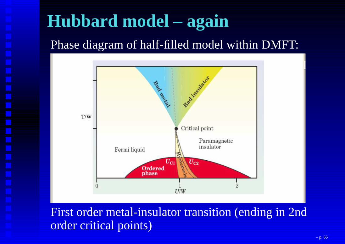
Hubbard model – againPhase diagram of half-filled model within DMFT:
First order metal-insulator transition (ending in 2ndorder critical points)
– p. 65
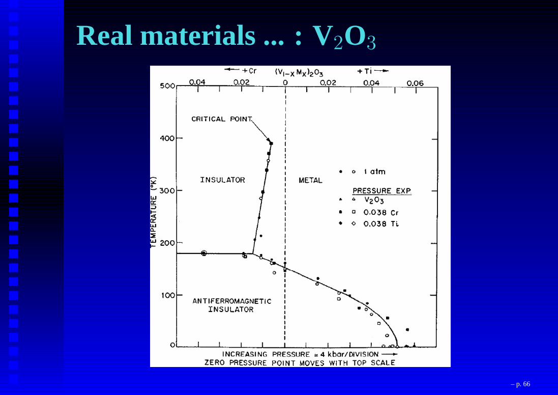
Real materials ... : V2O3
– p. 66

Wanted: ...... materials-specific calculations
– p. 67
– p. 68

The densityas a basic variable:Given a many-body wave function
Ψ(r1, r2, ..., rN ) (5)
the electronic density is given by
n(r) = N
∫
|Ψ(r, r2, ..., rN )|2dr2...drN (6)
– p. 69

The Hohenberg-Kohn TheoremThe ground state density n(r) of a bound system ofinteracting electrons in some external potential v(r)
determines this potential uniquely (up to a constant).
Remarks:• In the case of a degenerate ground state:any
ground state density• Proof uses Rayleigh-Ritz variational principle:
see Noble lecture in Rev. Mod. Phys. by W.Kohn or do it as an exercise!
– p. 70
InterpretationTwo different external potentials, sayvCu(r) andvNi(r), cannot have the same ground state density.→ One-to-one-correspondance between the externalpotential and the ground state density:
v(r) ↔ n(r)
Since v(r) determines the Hamiltonian:Ground state properties of an interactingmany-electron system arefunctionals of the densityonly.
– p. 71

Density functional theoryVariational principle:Define the universal functional
F [n] = minΨ→n〈Ψ|T + Vee|Ψ〉 (7)
Hohenberg-Kohn variational principle:
E[n] = F [n] +
∫
drVext(r)n(r) ≥ E0 (8)
F [n0] +
∫
drVext(r)n0(r) = E0 (9)
wheren0 is the exact ground state density.
– p. 72

Why is this useful?Energy = functional of the densityn(r):
E[n(r)] = T0[n(r)]+Eexternal[n(r)]+EHartree[n(r)]+Exc[n(r)]
T0[n(r)] = kinetic energy of anon-interacting referencesystem
(“Kohn-Sham system”) of densityn(r)
Schrödinger equation for the reference system (“Kohn-Sham
equation”):(
−12∆+ veff
)
φl(r) = ǫlφl(r)
“Kohn-Sham orbitals”φl parametrize the density:∑
occ |φl(r)|2 = n(r)
(Hohenberg& Kohn (1964), Kohn& Sham (1965))
– p. 73

Approximations forExc required, e.g. the “local density
approximation” (LDA):
ELDAxc [n(r)] =
∫
drn(r)ǫHEGxc (n(r))
(Hohenberg& Kohn (1964), Kohn& Sham (1965))
– p. 74

Density Functional Theory ...... within the local density approximation (LDA)
→ most commonly used method in modern electronic structurecalculations
• Band structures, densities of states, spectral properties
• Total energy calculations
• Phonons
• Magnetic exchange constants
• used within Molecular Dynamics
• ...
– p. 75
Density functional theory ...... achieves a mapping onto a separable system(mapping of interacting system onto non-interactingsystem of the same densityin an effective potential)for the ground state.
• effective potential unknown => local densityapproximation
• strictly speaking: not for excited states
In practice (and with the above caveats):DFT-LDA can be viewed as a specific choice forone-particle (band) theory
– p. 76

The N particle problem ...and its mean-field solution:N-electron Schrödinger equation
HNΨ(r1, r2, ..., rN ) = ENΨ(r1, r2, ..., rN )
with
HN = HkineticN +Hexternal
N +1
2
∑
i6=j
e2
|ri − rj|
becomes separable in mean-field theory:
HN =∑
i
hi
– p. 77
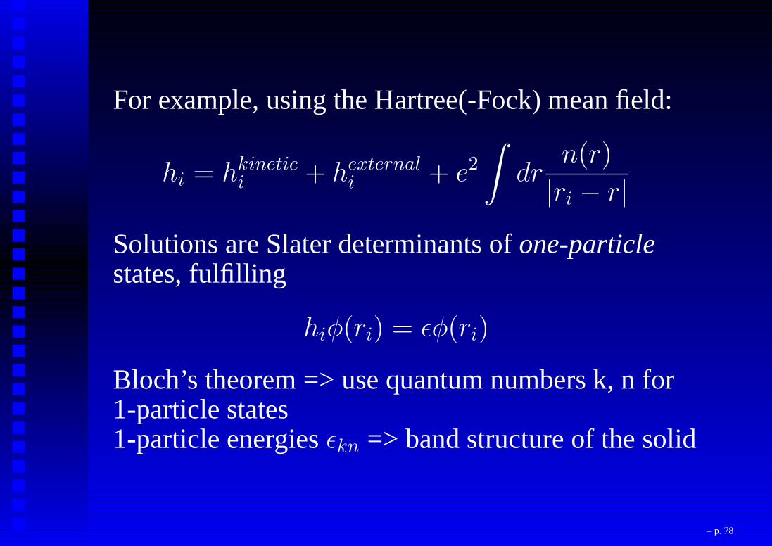
For example, using the Hartree(-Fock) mean field:
hi = hkinetici + hexternal
i + e2∫
drn(r)
|ri − r|
Solutions are Slater determinants ofone-particlestates, fulfilling
hiφ(ri) = ǫφ(ri)
Bloch’s theorem => use quantum numbers k, n for1-particle states1-particle energiesǫkn => band structure of the solid
– p. 78

Density functional theory ...... achieves a mapping onto a separable system(mapping of interacting system onto non-interactingsystem of the same densityin an effective potential)for the ground state.However:
• effective potential unknown => local densityapproximation
• strictly speaking: not for excited states
In practice (and with the above caveats):DFT-LDA can be viewed as a specific choice for amean field
– p. 79
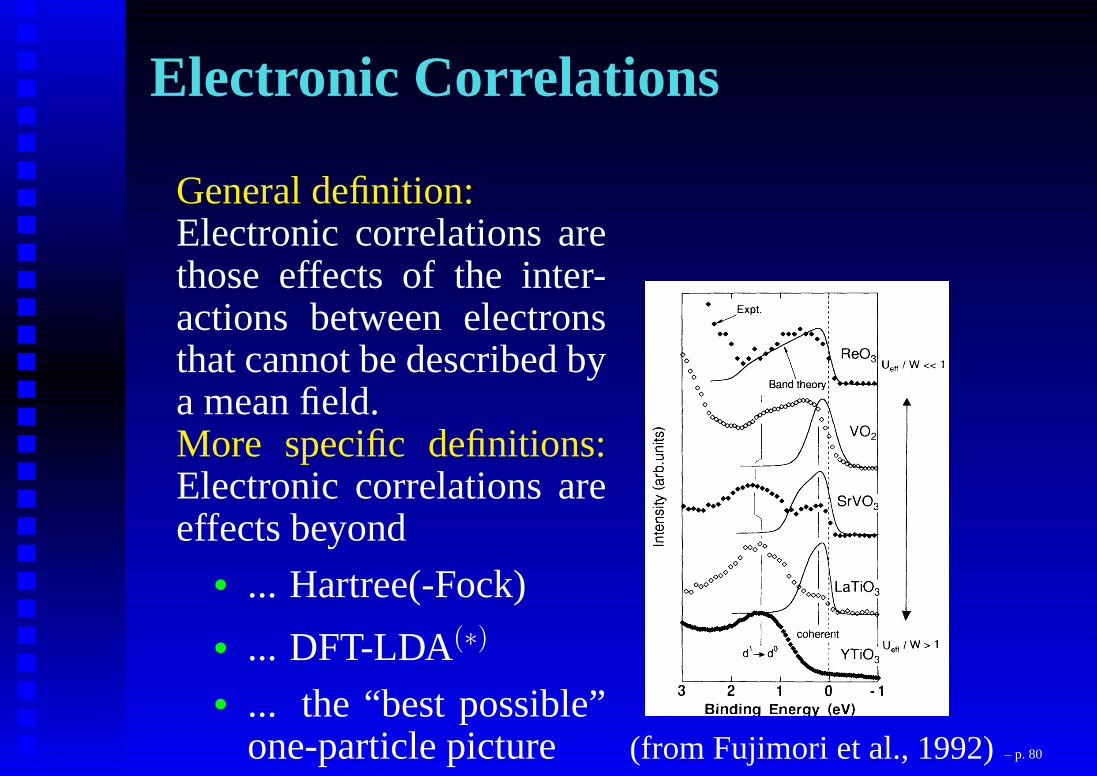
Electronic Correlations
General definition:Electronic correlations arethose effects of the inter-actions between electronsthat cannot be described bya mean field.More specific definitions:Electronic correlations areeffects beyond
• ... Hartree(-Fock)
• ... DFT-LDA(∗)
• ... the “best possible”one-particle picture (from Fujimori et al., 1992)– p. 80
Two regimes of failures of LDA1. “weak coupling”: moderate correlations,perturbative approaches work (e.g. “GWapproximation”)
2. “strong coupling”: strong correlations,non-perturbative approaches needed (e.g dynamicalmean field theory)
NB. Traditionally two communities, different techniques,butwhich in recent years have started to merge ...
NB. Correlation effects can show up in somequantities more than in others!
– p. 81
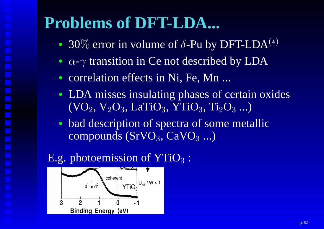
Problems of DFT-LDA...• 30% error in volume ofδ-Pu by DFT-LDA(∗)
• α-γ transition in Ce not described by LDA• correlation effects in Ni, Fe, Mn ...• LDA misses insulating phases of certain oxides
(VO2, V2O3, LaTiO3, YTiO3, Ti2O3 ...)• bad description of spectra of some metallic
compounds (SrVO3, CaVO3 ...)
E.g. photoemission of YTiO3 :
(Fujimori et al.)
– p. 82

Realistic Approach to CorrelationsCombine DMFT with band structure calculations
(Anisimov et al. 1997, Lichtenstein et al. 1998)
→ effective one-particle Hamiltonian within LDA→ represent in localized basis→ add Hubbard interaction term for correlatedorbitals→ solve within Dynamical Mean Field Theory
– p. 83

LDA+DMFT
H =∑
imσ
(HLDAim,i′m′ −Hdouble counting
im,i′m′ )a+imσai′m′σ
+1
2
∑
imm′σ (correl. orb.)
U imm′nimσnim′−σ
+1
2
∑
im6=m′σ (correl. orb.)
(U imm′ − J i
mm′)nimσnim′σ
→ solve withing DMFT
– p. 84
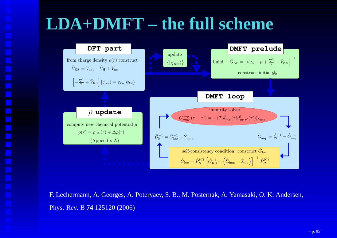
LDA+DMFT – the full scheme
DMFT loop
DMFT preludeDFT part
update
VKS = Vext + VH + Vxc
[
−∇2
2 + VKS
]
|ψkν〉 = εkν |ψkν〉
from charge density ρ(r) constructupdate
|χRm
〉 build GKS =[
iωn + µ+ ∇2
2 − VKS
]−1
construct initial G0
impurity solver
Gimpmm′(τ − τ ′) = −〈T dmσ(τ)d†
m′σ′(τ ′)〉Simp
self-consistency condition: construct Gloc
G−10 = G−1
loc + Σimp
Gloc = P(C)R
[
G−1KS −
(
Σimp − Σdc
)]−1
P(C)R
Σimp = G−10 − G−1
imp
ρ
compute new chemical potential µ
ρ(r) = ρKS(r) + ∆ρ(r)
(Appendix A)
F. Lechermann, A. Georges, A. Poteryaev, S. B., M. Posternak, A. Yamasaki, O. K. Andersen,
Phys. Rev. B74125120 (2006)
– p. 85
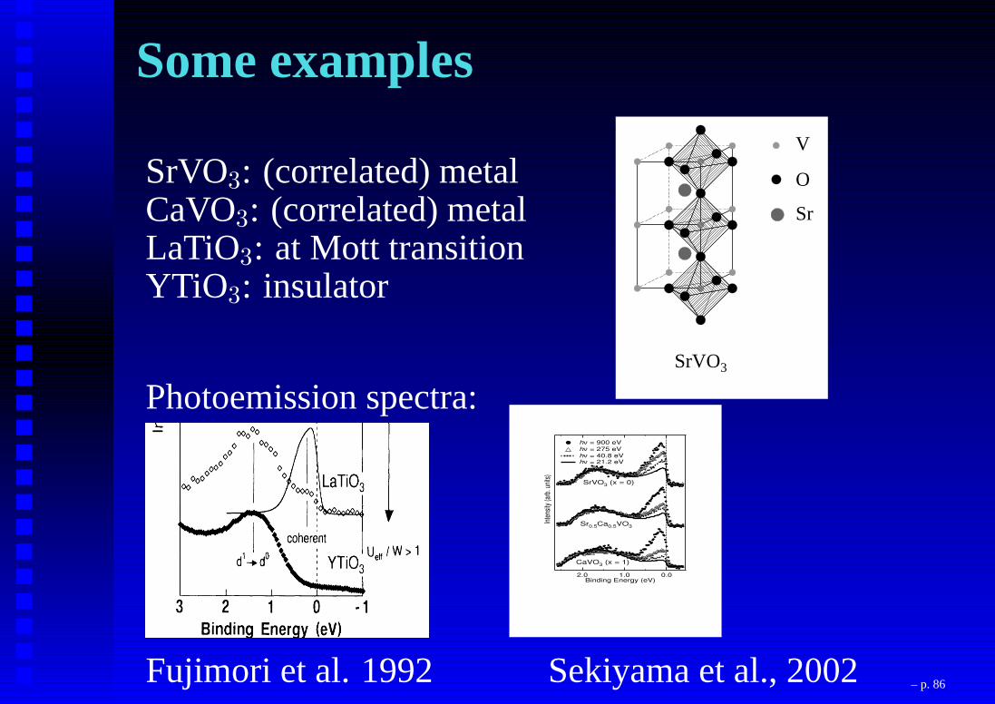
Some examples
SrVO3: (correlated) metalCaVO3: (correlated) metalLaTiO3: at Mott transitionYTiO3: insulator
3.1 Introduction 69
SrVO3
b)V
O
Sr
Figure 3.1: The crystal structure of (a) CaVO3 and (b) SrVO3 exhibiting various V-O-Vbond angles in the system.(= 180o) (see Fig. 3.1(b)) with cubic perovskite structure in SrVO3. Stoichiometric CaVO3and SrVO3 are both Pauli-paramagnetic metals [12-14]. Oxygen non-stoichiometry inCaVO3 leads to antiferromagnetic [15] or Curie-Weiss paramagnetic [16] behavior withno long range magnetic order down to 4 K. A solid solution of CaVO3 and SrVO3 can beformed over the entire composition range (0 x 1) with the formula Ca1xSrxVO3.Ca and Sr being homovalent (2+) in the solid solution, there is no change in the chargecarrier concentration with composition (x) and it is always one electron per V-ion acrossthe series. On the other hand, the dierent V-O-V bond angle results in dierent V-O-V hopping interaction strength, t. Thus, the eective correlation strength as measuredby U=W where W (/ t) denotes the bare bandwidth of the system, can be continuouslytuned by changing x, with CaVO3 being a more correlated metal with a larger U=W valuethan SrVO3 [11]. Thus, these compounds represent a well-suited experimental realizationof a continuous tuning of U=W and consequently, provide a good testing ground for thepredictions of the Hubbard model.With this in view, the electronic structure of Ca1xSrxVO3 was probed for severalvalues of x using photoelectron spectroscopy [11]. The experimental results are shown tobe incompatible with the existing theoretical results described in terms of the Hubbard
Photoemission spectra:
Inte
nsity
(arb
. uni
ts)
2.0 1.0 0.0Binding Energy (eV)
Sr0.5Ca0.5VO3
SrVO3 (x = 0)
CaVO3 (x = 1)
hν = 900 eV hν = 275 eV hν = 40.8 eV hν = 21.2 eV
Fujimori et al. 1992 Sekiyama et al., 2002 – p. 86

LDA+DMFT: spectra of perovskites
-4 -3 -2 -1 0 1 2 3 4 5 6
E(eV)
-4 -3 -2 -1 0 1 2 3 4 5 6
E(eV)
-4 -3 -2 -1 0 1 2 3 4 5 6
E(eV)
0
0.2
0.4
0.6
0.8
1
-4 -3 -2 -1 0 1 2 3 4 5 6
DO
S/s
tate
s/eV
/spi
n/ba
nd
E(eV)
0
0.2
0.4
0.6
0.8
1
-4 -3 -2 -1 0 1 2 3 4 5 6
DO
S/s
tate
s/eV
/spi
n/ba
nd
E(eV)
0
0.2
0.4
0.6
0.8
1
-4 -3 -2 -1 0 1 2 3 4 5 6
DO
S/s
tate
s/eV
/spi
n/ba
nd
E(eV)
0
0.2
0.4
0.6
0.8
1
DO
S s
tate
s/ev
/spi
n/ba
nd
0
0.2
0.4
0.6
0.8D
OS
sta
tes/
ev/s
pin/
band
0
0.2
0.4
0.6
0.8
1
DO
S s
tate
s/ev
/spi
n/ba
nd J=0.68 eVJ=0.68 eV
J=0.64 eV J=0.64 eV
U=5 eV
U=5 eVU=5 eV
YTiO3LaTiO3
SrVO3 CaVO3
U=5 eV
(E. Pavarini, S. B. et al., Phys. Rev. Lett.92176403 (2004) )– p. 87

Spectra of perovskites
SrVO3 LDA+DMFT
-4 -3 -2 -1 0 1binding energy
0.00
0.05
0.10
0.15
0.20
0.25
I(ω
)
U = 3.50 eVU = 3.75 eVU = 4.00 eV
Photoemission
Inte
nsi
ty (
arb
. units
)
2.0 1.0 0.0Binding Energy (eV)
Sr0.5Ca0.5VO3
SrVO3 (x = 0)
CaVO3 (x = 1)
hν = 900 eV hν = 275 eV hν = 40.8 eV hν = 21.2 eV
(see also Sekiyama et al. 2003,Lechermann et al. 2006)
– p. 88
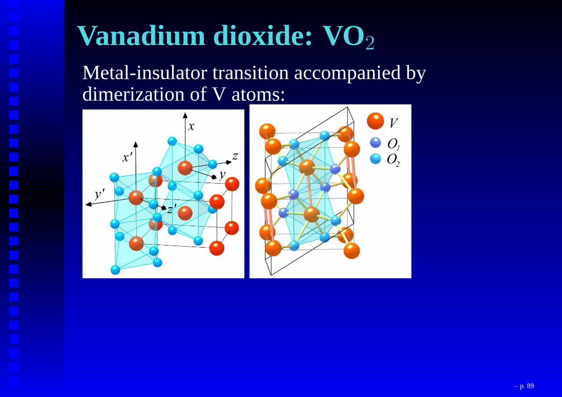
Vanadium dioxide: VO2
Metal-insulator transition accompanied bydimerization of V atoms:
– p. 89

VO2: Peierls or Mott ?
– p. 90

How far do we get ...... using Density Functional Theory for VO2 ?
metallic phase
-8
-6
-4
-2
0
2
4
6
8
Γ X R Z Γ R A Γ M A Z
(E -
EF)
(eV
)
”insulating“ phase
-2
-1
0
1
2
3
4
5
6
Γ Y C Z Γ A E Z Γ B D Z
(E -
EF)
(eV
)
DFT-LDA : no incoherent weight not insulating
(from V. Eyert)
– p. 91

VO2 : the physical pictureCharge transfereπg → a1g and bonding-antibonding splitting
metallic phase:
0.1
1
ω [e
V]
ΓZCYΓ-2
-1
0
1
2
3
insulating phase:
0.1
1
ω [e
V]
Γ Y C Z Γ-2
-1
0
1
2
3
Spectral functions and “band structure”
det(
ωk + µ−HLDA (k)−ℜΣ(ωk))
= 0
J.M. Tomczak, S.B., J.Phys.:Cond.Mat. 2007; J.M. Tomczak,F. Aryasetiawan, S.B., PRB 2008
– p. 92

VO2 monoclinic phase
quasi-particle poles (solutions ofdet[ω + µ−H(k)− Σ(ω)]=0) and band structurefrom effective (orbital-dependent) potential
(→ for spectrum of insulating VO2: independentparticle picture not so bad!! (but LDA is!)) – p. 93

Optical Conductivity of VO 2
0
1
2
3
4
5
6
0 0.5 1 1.5 2 2.5 3 3.5 4 4.5 5 5.5
Re
σ(ω
) [1
03 (Ω
cm)-1
]
ω [eV]
Metal
Theory
Exp. (i)
Exp. (ii)
Exp. (iii)
0
1
2
3
4
5
6
0 0.5 1 1.5 2 2.5 3 3.5 4 4.5 5 5.5
Re
σ(ω
) [1
03 (Ω
cm)-1
]
ω [eV]
TheoryE || [001]E || [1-10]E || [aab]
0
1
2
3
4
5
6
0 0.5 1 1.5 2 2.5 3 3.5 4 4.5 5 5.5
Re
σ(ω
) [1
03 (Ω
cm)-1
]
ω [eV]
Theory
Experiments
Insulator
Verleur et al. E || [001]Verleur et al. E ⊥ [001]Okazaki et al.Qazilbash et al.
0
1
2
3
4
5
6
0 0.5 1 1.5 2 2.5 3 3.5 4 4.5 5 5.5
Re
σ(ω
) [1
03 (Ω
cm)-1
]
ω [eV]
Theory
Experiments
Insulator
Verleur et al. E || [001]Verleur et al. E ⊥ [001]Okazaki et al.Qazilbash et al.
[Verleur et al.] : single crystals
[Okazakiet al.] : thin filmsE ⊥ [001], Tc=290 K
[Qazilbashet al.] : polycrystalline films, preferential
E ⊥ [010], Tc=340 K
– p. 94

Cerium fluorosulfide CeFS
Mott insulator,paramagnetic
Need to treat both, localised f-states and delocalisedp-electrons→ How to incorporate atomic physics intoelectronic structure theory ?
– p. 95
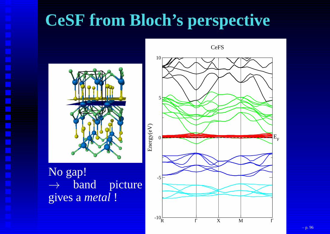
CeSF from Bloch’s perspective
No gap!→ band picturegives ametal!
R Γ X M Γ-10
-5
0
5
10
Ene
rgy(
eV)
CeFS
EF
– p. 96
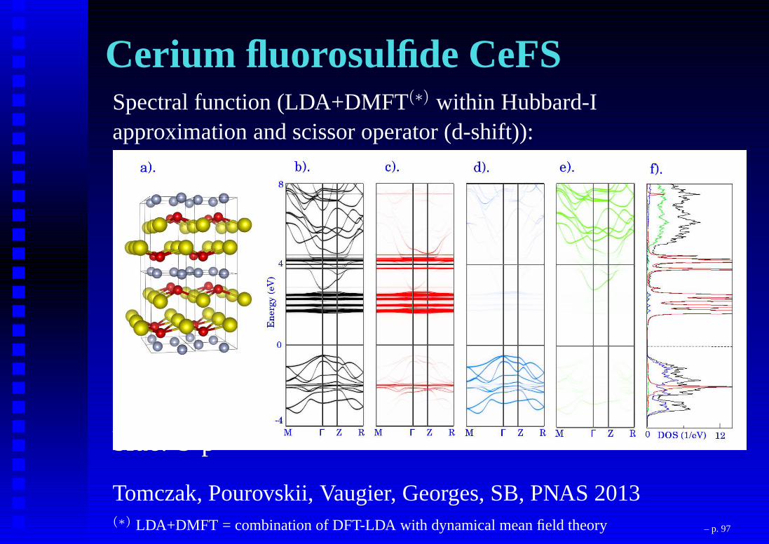
Cerium fluorosulfide CeFSSpectral function (LDA+DMFT(∗) within Hubbard-Iapproximation and scissor operator (d-shift)):
red: Ce-4fgreen: Ce-5dblue: S-p
Tomczak, Pourovskii, Vaugier, Georges, SB, PNAS 2013(∗) LDA+DMFT = combination of DFT-LDA with dynamical mean field theory – p. 97

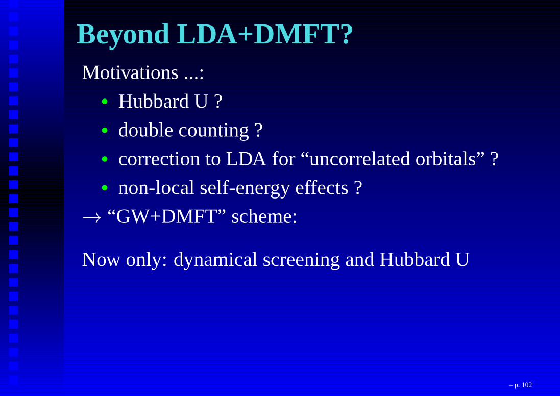
Beyond LDA+DMFT?Motivations ...:
• Hubbard U ?• double counting ?• correction to LDA for “uncorrelated orbitals” ?• non-local self-energy effects ?
→ “GW+DMFT” scheme
– p. 98
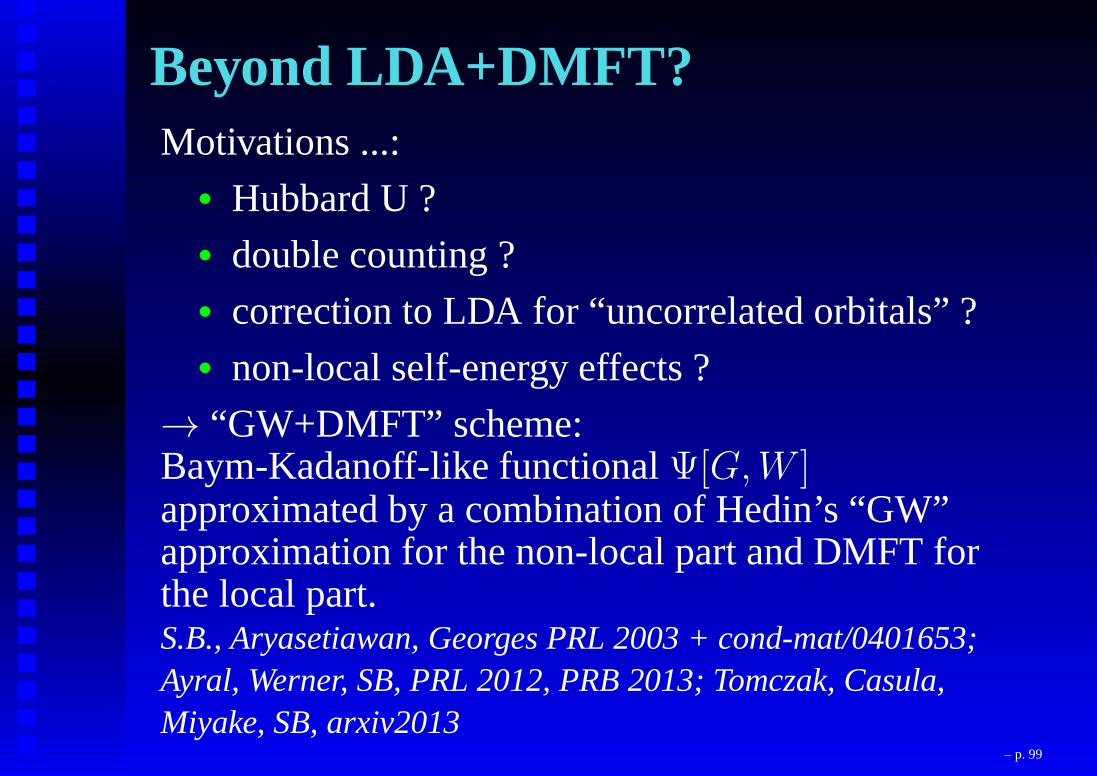
Beyond LDA+DMFT?Motivations ...:
• Hubbard U ?• double counting ?• correction to LDA for “uncorrelated orbitals” ?• non-local self-energy effects ?
→ “GW+DMFT” scheme:Baym-Kadanoff-like functionalΨ[G,W ]approximated by a combination of Hedin’s “GW”approximation for the non-local part and DMFT forthe local part.S.B., Aryasetiawan, Georges PRL 2003 + cond-mat/0401653;Ayral, Werner, SB, PRL 2012, PRB 2013; Tomczak, Casula,Miyake, SB, arxiv2013
– p. 99
The representability point of viewRepresentphysical quantity of interest of real systemby an effective model, with effective quantities
Quantity – Model – Auxiliary quantity:• Density Functional Theory:
Density – non-interacting system –(Kohn-Sham-) potential
• DMFT:local Green’s function G – impurity model– Weiss fieldG0
• GW+DMFT: as in DMFT, but in addition:screened local Coulomb interactionWloc –impurity model with dynamical interaction –(dynamical) HubbardU
– p. 100
Can we calculate ...... Wlocal from a (dynamical) impurity model?
→ Question of representability !• DMFT: Glocal calculated from impurity model• What aboutWlocal ?
Self-consistency requirement:• Gimpurity = Glocal of the solid• Wimpurity = Wlocal of the solid
→ “GW+DMFT”(S.B., F. Aryasetiawan, A. Georges PRL90086402 (2003) +cond-mat/0401653)
– p. 101
Beyond LDA+DMFT?Motivations ...:
• Hubbard U ?• double counting ?• correction to LDA for “uncorrelated orbitals” ?• non-local self-energy effects ?
→ “GW+DMFT” scheme:
Now only: dynamical screening and Hubbard U
– p. 102

What’s U in a solid?A simpler answer ?
– p. 103
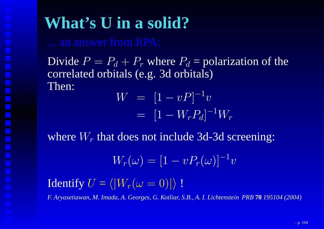
What’s U in a solid?... an answer from RPA:
DivideP = Pd + Pr wherePd = polarization of thecorrelated orbitals (e.g. 3d orbitals)Then:
W = [1− vP ]−1v
= [1−WrPd]−1Wr
whereWr that does not include 3d-3d screening:
Wr(ω) = [1− vPr(ω)]−1v
IdentifyU = 〈|Wr(ω = 0)|〉 !F. Aryasetiawan, M. Imada, A. Georges, G. Kotliar, S.B., A. I. Lichtenstein PRB70195104 (2004)
– p. 104

What’s U in a solid?... an answer from RPA:
DivideP = Pd + Pr wherePd = polarization of thecorrelated orbitals (e.g. 3d orbitals)Then:
W = [1− vP ]−1v
= [1−WrPd]−1Wr
whereWr that does not include 3d-3d screening:
Wr(ω) = [1− vPr(ω)]−1v
IdentifyU(ω) = 〈|Wr(ω)|〉 !
– p. 105

Example: SrVO3
0 2 4 6 8 10 12 14 16 18 20 22 24 26 28 30omega (eV)
-18
-15
-12
-9
-6
-3
0
3
6
9
12
15
18
21
24U
(eV
)
t2gdpt2g+pVbar for t2g model
SrVO3
– p. 106
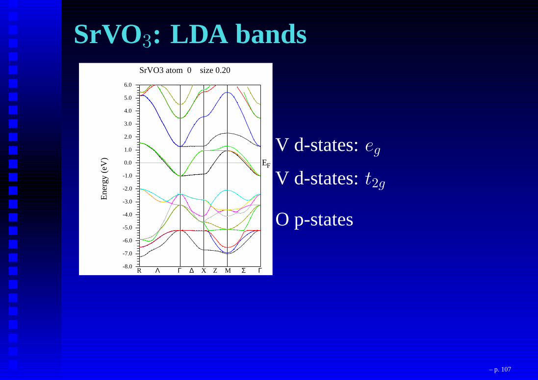
SrVO3: LDA bandsSrVO3 atom 0 size 0.20
R Λ Γ ∆ X Z M Σ Γ
E F
Ene
rgy
(eV
)
0.0
1.0
2.0
3.0
4.0
5.0
6.0
-1.0
-2.0
-3.0
-4.0
-5.0
-6.0
-7.0
-8.0
V d-states:eg
V d-states:t2g
O p-states
– p. 107
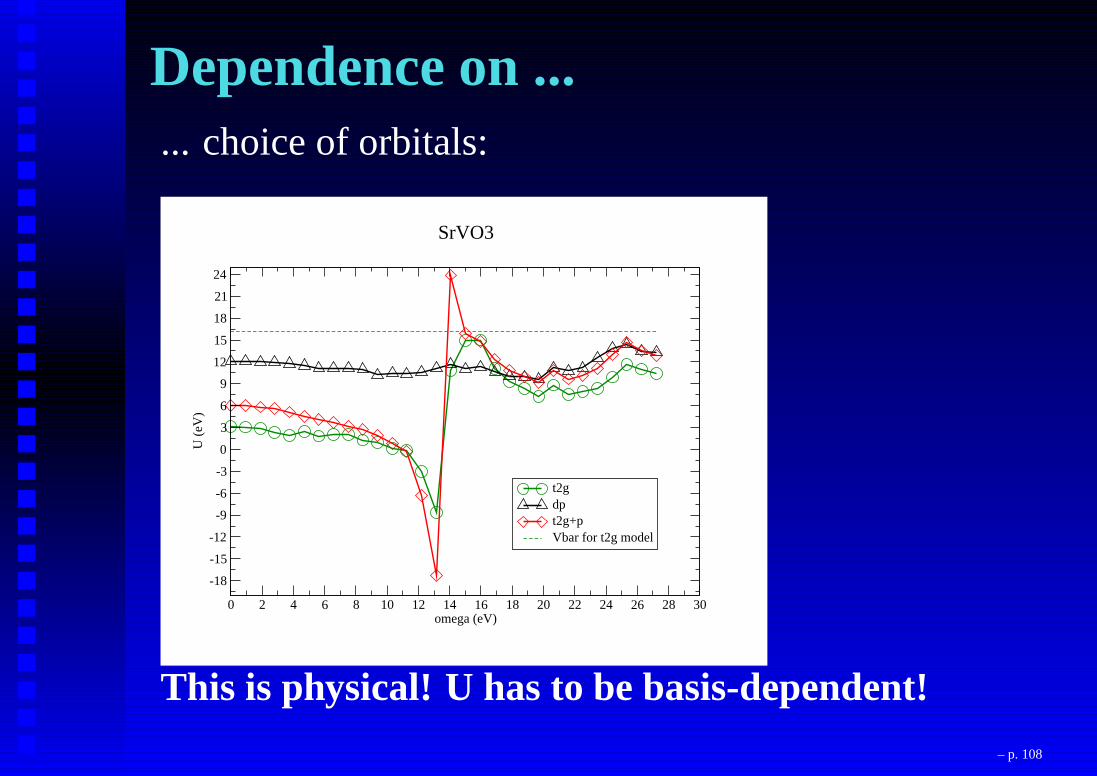
Dependence on ...... choice of orbitals:
0 2 4 6 8 10 12 14 16 18 20 22 24 26 28 30omega (eV)
-18
-15
-12
-9
-6
-3
0
3
6
9
12
15
18
21
24
U (
eV)
t2gdpt2g+pVbar for t2g model
SrVO3
This is physical! U has to be basis-dependent!
– p. 108
CRPAcan be viewed as an approximation to the calculationof U within a full GW+DMFT scheme!(S.B., F. Aryasetiawan, A. Georges PRL90086402 (2003) +cond-mat/0401653)What about “LDA+U(ω)+DMFT”?Casula, Rubtosv, SB., PRB 2012
– p. 109
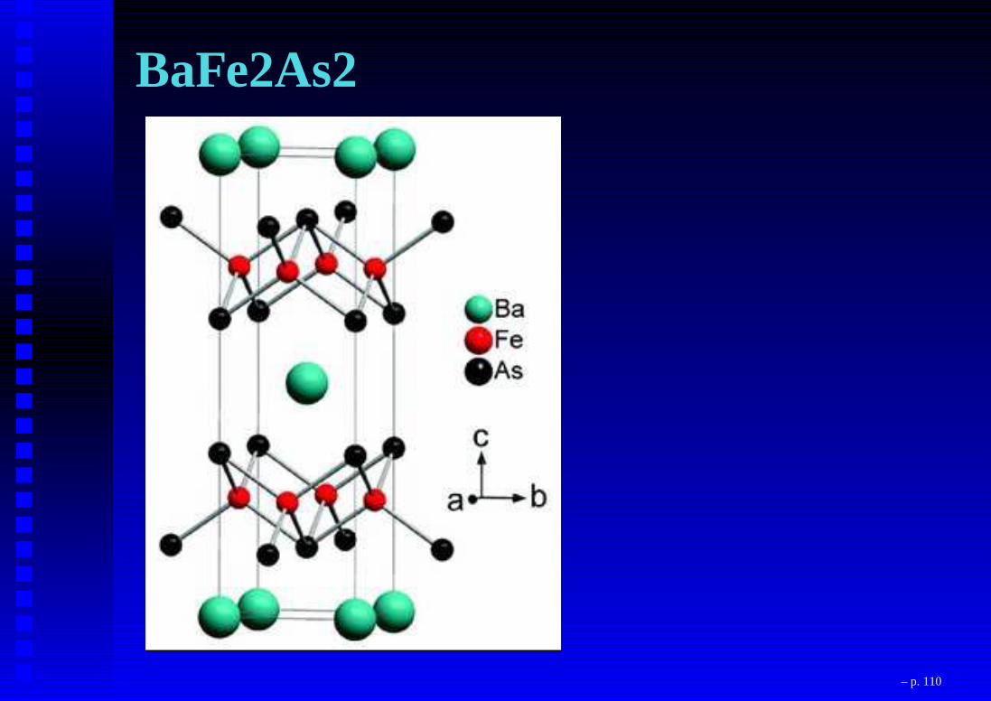
BaFe2As2
– p. 110

BaFe2As2
– p. 111
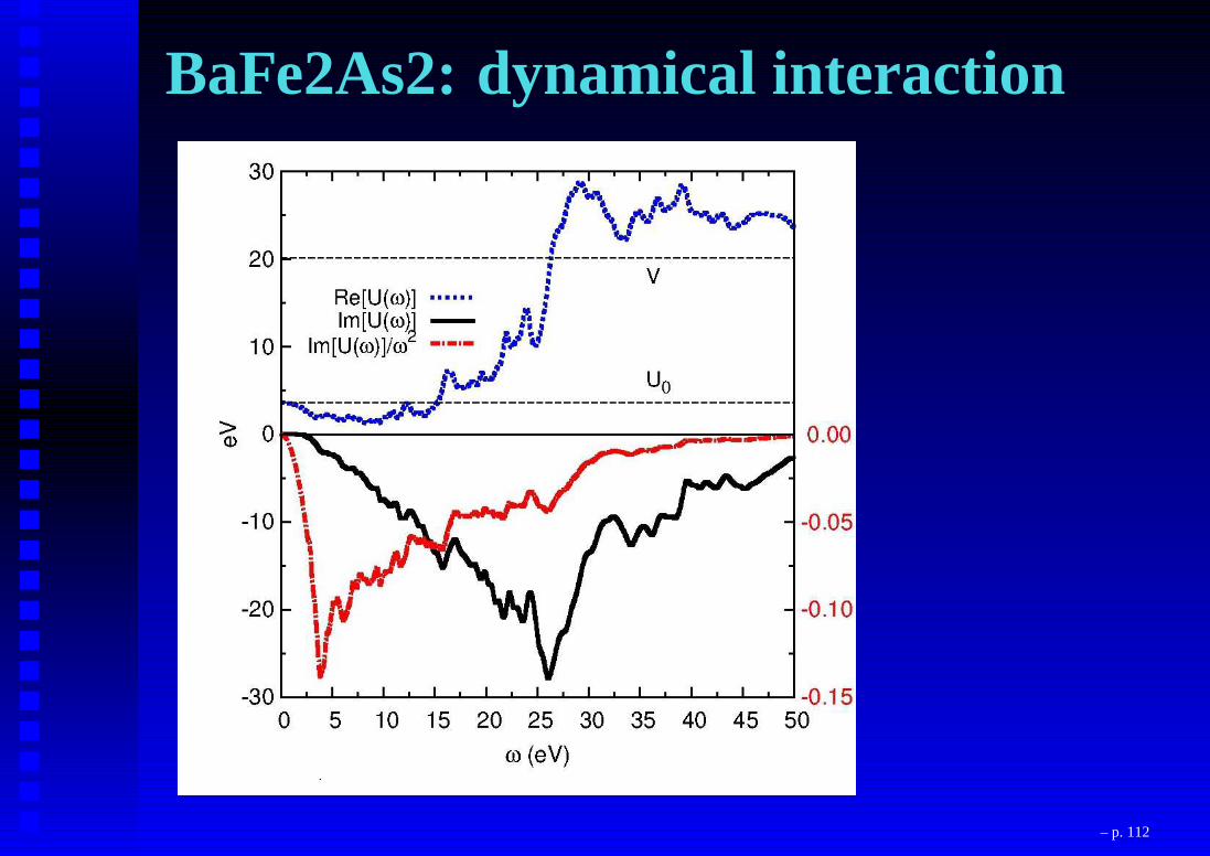
BaFe2As2: dynamical interaction
– p. 112

Ba1−xKxFe2As2: spectral function
Werner, Casula, Miyake, Aryasetiawan, Millis, SB, Nature Physics 2012 – p. 113
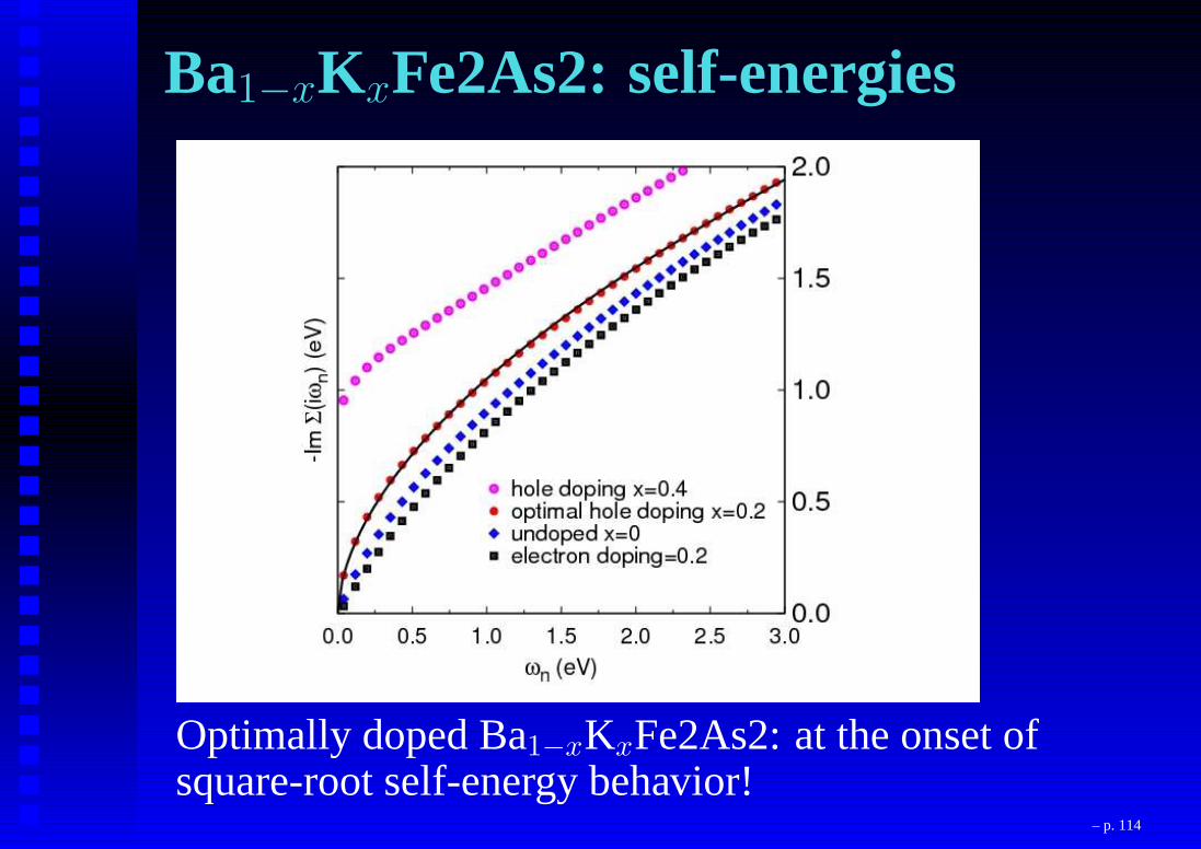
Ba1−xKxFe2As2: self-energies
Optimally doped Ba1−xKxFe2As2: at the onset ofsquare-root self-energy behavior!
– p. 114

Optimally doped Ba1−xKxFe2As2
Huge T-dependence! – p. 115
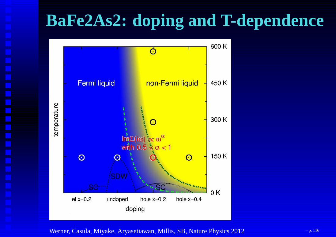
BaFe2As2: doping and T-dependence
Werner, Casula, Miyake, Aryasetiawan, Millis, SB, Nature Physics 2012 – p. 116
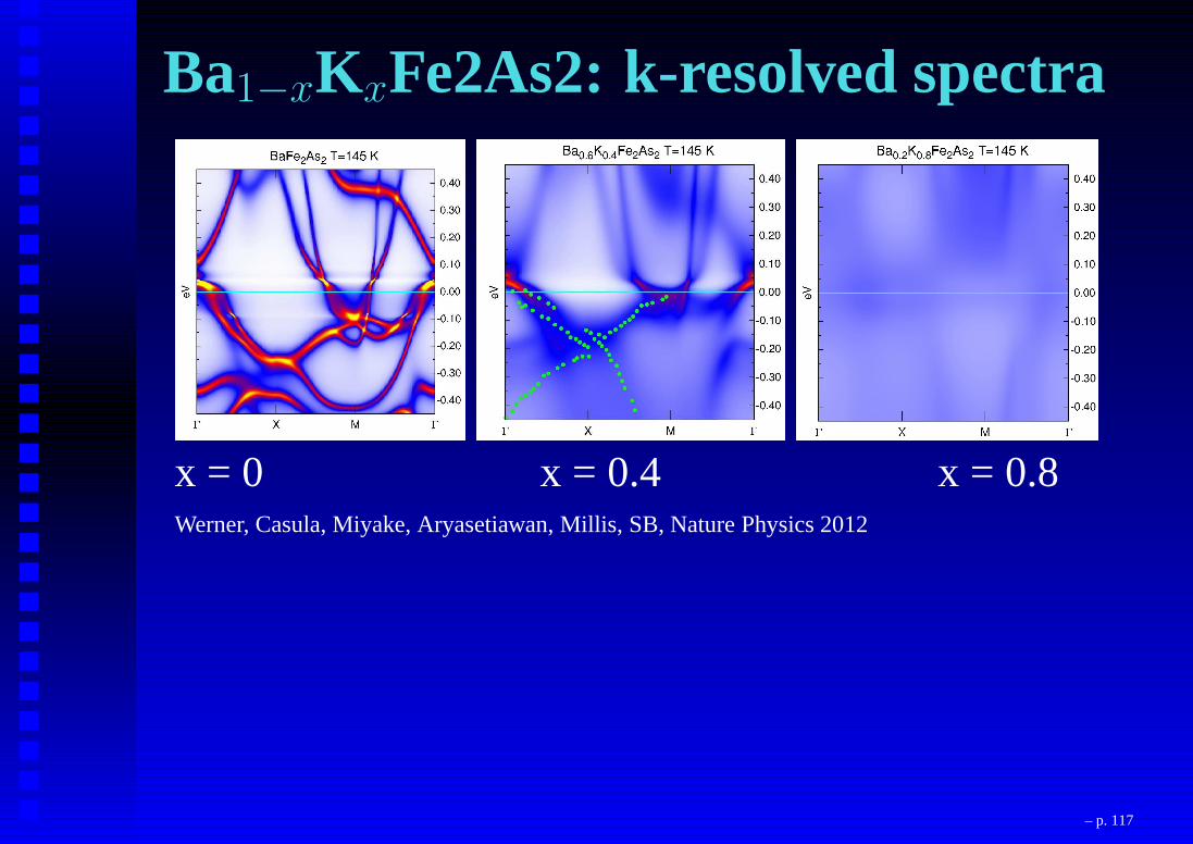
Ba1−xKxFe2As2: k-resolved spectra
x = 0 x = 0.4 x = 0.8Werner, Casula, Miyake, Aryasetiawan, Millis, SB, Nature Physics 2012
– p. 117
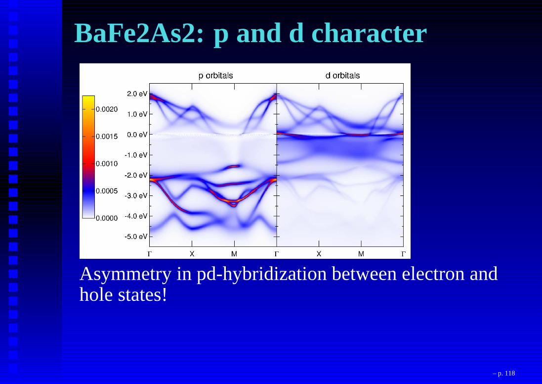
BaFe2As2: p and d character
Asymmetry in pd-hybridization between electron andhole states!
– p. 118

Conclusions?
– p. 119

Not everything ...... depends only on the average occupation!
– p. 120

Not everything ...... depends only on the average occupation!
– p. 121
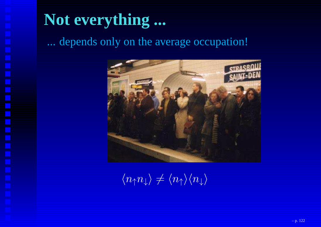
Not everything ...... depends only on the average occupation!
〈n↑n↓〉 6= 〈n↑〉〈n↓〉
– p. 122
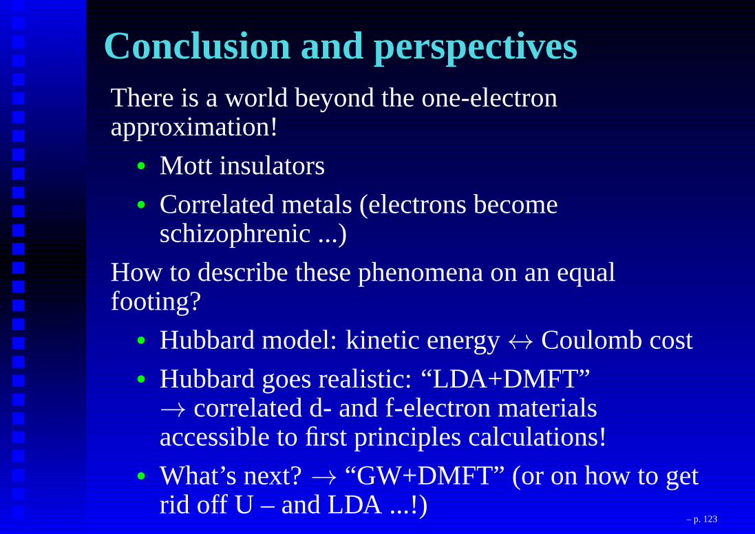
Conclusion and perspectivesThere is a world beyond the one-electronapproximation!
• Mott insulators• Correlated metals (electrons become
schizophrenic ...)
How to describe these phenomena on an equalfooting?
• Hubbard model: kinetic energy↔ Coulomb cost• Hubbard goes realistic: “LDA+DMFT”→ correlated d- and f-electron materialsaccessible to first principles calculations!
• What’s next?→ “GW+DMFT” (or on how to getrid off U – and LDA ...!)
– p. 123
Useful Reading (not complete)
• DMFT - Review:
A. Georges et al., Rev. Mod. Phys., 1996
• LDA+DMFT - Reviews:
G. Kotliar et al., Rev. Mod. Phys. (2007)
D. Vollhardt et al., J. Phys. Soc. Jpn. 74, 136 (2005)
A. Georges, condmat0403123
S. Biermann, in Encyclop. of Mat. Science. and Technol.,
Elsevier 2005.F. Lechermann et al., Phys. Rev. B74125120 (2006)
– p. 124
References, continuedSome recent applications of LDA+DMFT:
• VO2: J. Tomczak, S.B., Psik-Newsletter, Aug. 2008, J.
Phys. Cond. Mat. 2007; EPL 2008, PRB 2008, Phys. stat.
solidi 2009.
J. Tomczak, F. Aryasetiawan, S.B., PRB 2008;
S.B., A. Poteryaev, A. Georges, A. Lichtenstein, PRL 2005
• V2O3: A. Poteryaev, J. Tomczak, S.B., A. Georges, A.I.
Lichtenstein, A.N. Rubtsov, T. Saha-Dasgupta, O.K.
Andersen, PRB 2007.
• Cerium: Amadon, S. B., A. Georges, F. Aryasetiawan, PRL
2006
• d1 Perovskites: E. Pavarini, S. B. et al., PRL 2004– p. 125

– p. 126
![Index [users.physik.fu-berlin.de]users.physik.fu-berlin.de/~kleinert/b5/psfiles-sp/pthic... · 2014. 8. 7. · 1620 Index Babaev, E. .....x Babcenco, A. .....617, 1027 Bachelier,](https://static.documents.pub/doc/80x56/6086050bfe80cf0c283eca81/index-users-users-kleinertb5psfiles-sppthic-2014-8-7-1620-index.jpg)


