Similarity in Perception: A W indow to Brain …ruppin/similarity.pdfSimilarity in Perception: A W...

Similarity in Perception: A Window to Brain Organization

Zach Solan

School of Physics and Astronomy

Tel Aviv University, Tel Aviv 69978, Israel

[email protected]

Eytan Ruppin*

School pf Mathematics and School of Medicine

Departments of Computer Science & Physiology

Tel Aviv University, Tel Aviv 69978, Israel

[email protected]

June 6, 1999

Abstract

This paper presents a neural model of similarity perception in identification tasks. It is

based on self-organizing maps and population coding and is examined through five different

identification experiments. Simulating an identification task, the neural model generates a

confusion matrix that can be compared directly with that of human subjects. The model

achieves a fairly accurate match with the pertaining experimental data both during training

and thereafter. To achieve this fit, we find that the entire activity in the network should

decline while learning the identification task, and that the population encoding of the specific

stimuli should become sparse as the network organizes. Our results thus suggest that a

self-organizing neural model employing population coding can account for identification

processing, while suggesting computational constraints on the underlying cortical networks.

* To whom correspondence should be addressed.

Similarity in Perception: A window to brain development 1

INTRODUCTION

Similarity is a basic concept in cognitive psychology which is utili zed to explore the

principles of perception. Theories about similarity aim at explaining when people

identify or judge two different stimuli as related (e.g: Ashby & Perrin, 1988; Ashby &

Lee, 1991). Experimentally, similarity between objects is measured using different kinds

of stimuli and modaliti es, via two fundamental methods. The first is the direct method,

where subjects are asked to explicitl y estimate the level of similarity between two

objects. The second method is the indirect one, where subjects are asked to identify

various stimuli . This method is motivated by the basic assumption that two similar

objects tend to be confused more often. In this paper we focus on modeling similarity

experiments performed with the indirect method, which is less dependent on attentional

levels. Indirect similarity experiments are also performed in animals, making relevant

neurophysiological data readily available.

In a typical indirect similarity experiment, the stimuli are presented to the subject

in random order. The subject’s task is to identify each stimulus by its serial number, and

report it as the subject response. In case of error in identification, the experimenter

informs the subject about the correct answer. The data thus obtained is typically

represented in a two dimensional square confusion matrix. A cell i n row i and column j

of the confusion matrix reports the number of times the subject has erroneously identified

stimulus i as stimulus j, and the number of the correct responses is reported on the

diagonal. Similarity experiments can be categorized by three major characteristics: the

modaliti es involved, the features that construct the stimuli , and the dimension (the

number of features) of the stimuli . The similarity experiments modeled in this paper, a


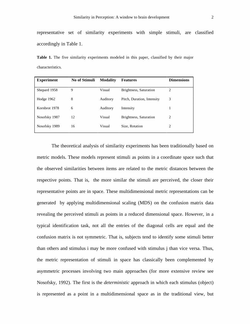
representative set of similarity experiments with simple stimuli , are classified

accordingly in Table 1.

Table 1. The five similarity experiments modeled in this paper, classified by their major

characteristics.

Experiment No of Stimuli Modality Features Dimensions

Shepard 1958 9 Visual Brightness, Saturation 2

Hodge 1962 8 Auditory Pitch, Duration, Intensity 3

Kornbrot 1978 6 Auditory Intensity 1

Nosofsky 1987 12 Visual Brightness, Saturation 2

Nosofsky 1989 16 Visual Size, Rotation 2

The theoretical analysis of similarity experiments has been traditionally based on

metric models. These models represent stimuli as points in a coordinate space such that

the observed similarities between items are related to the metric distances between the

respective points. That is, the more similar the stimuli are perceived, the closer their

representative points are in space. These multidimensional metric representations can be

generated by applying multidimensional scaling (MDS) on the confusion matrix data

revealing the perceived stimuli as points in a reduced dimensional space. However, in a

typical identification task, not all the entries of the diagonal cells are equal and the

confusion matrix is not symmetric. That is, subjects tend to identify some stimuli better

than others and stimulus i may be more confused with stimulus j than vice versa. Thus,

the metric representation of stimuli i n space has classically been complemented by

asymmetric processes involving two main approaches (for more extensive review see

Nosofsky, 1992). The first is the deterministic approach in which each stimulus (object)

is represented as a point in a multidimensional space as in the traditional view, but


employing an additional set of choice decision rules. An important representative of this

approach is the Multidimensional Scaling (MDS) choice model (Shepard 1957; Luce

1963), which has been able to account for both the asymmetric and the unequal self

identification characteristics of the data. According to this model, the probabilit y that

stimuli i i s identified as stimuli j i s an outcome of the choice model decision rule:

(1) ( )∑

=N LN�η

η

N

LMMLM E

E653

where LMη is the similarity between stimulus i and stimulus j, a decreasing monotonic

function (exponential or Gaussian) of the distance in perceptual space between stimulus i

and stimulus j. bj denotes bias parameters that are associated with each stimulus. The

model free parameters are the bias and the location of each stimulus in the

multi -dimensions perceptual space. Thus, the amount of free parameters scales linearly

with the number of stimuli and dimensions of the perceptual space.

In the second, probabili stic approach, each stimulus is represented as a statistical

ensemble of points. An important representative of this approach is General Recognition

Theory (GRT) (Ashby & Townsend, 1986; Ashby & Perrin, 1988). GRT is based on the

assumption that noise is an inherent component in the perceptual system. Hence, across

trials, the repeated presentation of the same stimulus gives rise to a probabili stic

distribution around the expected values of stimulus representations. In an identification

task, GRT assumes the subject divides the perceptual space into regions. In each trial the

subject determines within which decision boundaries the stimulus representation falls,

and this leads to the associated response. GRT accounts for the asymmetric nature of the

data by allotting regions of different sizes to the representation of different stimuli . In

order to fit the psychological data the model free parameters are the decision boundaries


for each stimulus and its location in the multi -dimensions perceptual space. These

approaches provide an excellent fit for the empirical data, but do not account for the

representation of similarity in neural terms. Moreover, these approaches embody a very

large number of parameters (a few tens) that should be explicitl y set to correctly fit the

data in a specific manner for each different experiment. As will become evident, the

model proposed in this paper points to an interesting connection between the MDS and

GRT models of identification.

Several attempts have been previously made to identify the neural correlates of

similarity perception in the brain (Edelman, 1995, 1997; Tadashi et al., 1998). A few

researchers have performed experiments of odor identification in rats (Youngentob et al.,

1990; Kent et al., 1995). They analyzed the perceptual odor stimulus space by applying

MDS analysis to a confusion matrix of f ive different odor stimuli , which resulted in a

reduced 2-dimensional space. Examining the neural activity of the olfactory mucosa

during odor inhalation, they found that each odorant had a unique "hot spot" region of

maximum sensitivity. A y preserving mapping between the position of the corresponding

odorant in the reduced 2-dimensional psychophysical odor space and the mucosa location

of these "hot spots" was identified. Wang et al. (1996) have investigated the functional

organization of object recognition, using optical imaging in inferotemporal cortex, again

finding a regional clustering of cells responding to similar features. Young and Yamane

(1992) have shown that the encoding of the visual perceptual space of familiar human

faces in the inferotemporal cortex of monkeys is population based. This population

encoding is sparse and is related to the spatial properties of face stimuli i n the

corresponding MDS psychophysical space. Put together, these findings support the

notion that the processing in some cortical regions engaged in perception employs both a


topological mapping and population coding. A model relating between topological

mapping and population coding has been previously suggested by Guenther & Gjaja,

(1996) in order to provide an explanation for the well known phenomenon of the

perceptual magnet effect (Kuhl, 1991). While Guenther & Gjaja’s, work models a

different set of data, their model of stimulus discriminabilit y has a close relation to

similarity perception, inferring perceptual stimulus relations from map activities. Their

model, as in our current paper, suggests that the perceptual effects observed in the

psychological experiments arise as a natural consequence of the formation and the

organization of the neural map.

The observation of Kent et al. (1995) that there is a topological mapping from the

perceptual similarity space to its representation in the olfactory mocusa, obviously raises

the question of the possible neural mechanisms underlying this phenomenon. A natural

candidate is the Self-Organizing Map (SOM) algorithm (Kohonen, 1982), which has

been shown (see Kaski 1997 for a review) to be strongly related to the MDS procedure,

both maintaining a structural topological mapping. The SOM algorithm, to be described

in detail i n the next section, has an explicit neural level realization. In this paper, we

study a neural model of similarity perception that is based on an SOM topological

mapping and population coding. As will be seen, the quest to model the psychophysical

data of similarity perception suggests useful constraints on the pertaining

neurophysiological level. The next section provides an overview of the model and our

simulation experiments. The Results section compares the computational results with the

human data. The last section discusses brain organization and development in lieu of our

results.


THE MODEL

Model Overview

The model is based on a self-organizing neural network (Kohonen, 1982, 1989) that is

implemented in computer simulations. In order to describe the model in a concrete

fashion, we refer to a typical indirect similarity experiment performed by Shepard

(1958). This well known experiment used 9 stimuli of distinct red colored chips of

uniform size. The colored chips, as specified by the system of Munsell , were of a

constant hue, but varied in brightness (4 levels) and saturation (4 levels of chroma). Each

chip was labeled by a number from “1” to “9” . After a short period of training, 36

subjects were asked to identify the exposed colored chips by their labels. In case of an

identification error, the experimenter provided the subject with the correct answer. Each

of the 36 subjects was exposed to a random sequence of 200 successive chip

identification trials and their responses were assembled in a typical 9X9 confusion matrix

(Table 2).

The model is composed of a network of laterally interacting neurons arranged in a

two-dimensional array, encoding distinct features of the input stimuli . The neurons are

fully connected to a common layer of input neurons as portrayed in Figure 1.


Figure 1. Schematic Model description. The neural model is composed of a two-dimensional array

of neurons full y connected to a common source of input fibers transmitting the input stimuli .

To simulate this experiment, the neural network was presented with 2-dimensional input

feature vectors representing the 9 stimuli of the original experiment. The value of each of

the two components of an input prototype vector was determined by the corresponding

feature value (i.e., brightness and saturation) of the stimulus it represents. To generate an

input vector a random noise term is added to each one of the prototype vector

components representing an external noisy environment.

When an input vector is presented and processed by the network, the

identification response of the neural model can be “ read” from its activity state. The

network responses to the representation of a set of stimuli are accumulated in a confusion

matrix in a standard manner. The readout of the output data is based on population

coding (Georgopoulos et al., 1982,1984). In contrast with the Winner-Take-All approach,

population coding is a method that determines the location of a response vector in the

network’s “perceptual” space as a function of the entire network’s activity and not the

�

�)HDWXUH��

U�Z�� Z��

,QSXW�)LEHUV�

;�,QSXW�9HFWRU�

,QSXW�1HXURQV�

5/�5DGLXV�RI�/HDUQLQJ�

�ZU�6\QDSWLF�:HLJKW�9HFWRU��RI�QHXURQ�U�5$�5DGLXV�RI�$FWLYLW\�

:LQQHU�QHXURQ�

)HDWXUH��[��[��

V�


result of a single neuron’s activity. The model’s operation consists of two conceptually

distinct phases: The training phase, during which the network gradually self-organizes,

extracting the regularities of the input stimuli , and the identifi cation (performance)

phase, during which the organized network can successfully simulate identification

tasks. Stimulus identification may also be performed during the training phase, to

simulate identification tasks performed early in the learning process.

The Training Phase

In the training phase, the ensemble of input vectors presented to the network is generated

according to the following process: A prototype feature vector representing one of the

stimuli i n the identification experiment is randomly selected. Then, to generate an input

vector x, a noise term is added to each of its n components representing an external noisy

environment (typically n=2 or 3, the noise is normally distributed with zero mean, fixed

variance and zero covariance). The magnitude of all the input vectors is kept normalized,

thus eliminating a scaling bias (see Appendix I for details). The presentation of an input

vector gives rise to excitation of neurons in the network array (see Figure 1). The

response of neuron r is specified by its n-dimensional synaptic weight vector wr and is

equal to the dot product of x⋅wr (Kohonen, 1989, 1993). In response to a given input

stimulus, the most active neuron in the lattice (for which x⋅wr is maximal) is defined as

the winner neuron, s. Its surrounding network activity is modulated by a Gaussian kernel

function ( )UK $5 centered on neuron s, whose variance RA

2 controls the radius of

activation around the winner ( ( )UK $5 is largest at r=s and declines monotonically to

zero with increasing distance between the s and the r’ th neuron),


(2) ( )

⋅−

−= �

�

�H[S$

5 5VUUK $ .

The activity mr of neuron r is defined as

(3) ( ) ( )UKP $5U ⋅⋅= UU

ZZ[[

.

During training, the network self-organizes by modifying the synaptic weights of the

neurons in the winner’s surroundings by

(4) ( ) ( )�ROG��ROG�

UU

�ROG��ROG�

UU

�QHZ��QHZ�

UU

ZZ;;ZZZZ

−⋅⋅+= UK /5ε

(5) ( )

⋅−

−= �

�

�H[S/

5 5VUUK / ,

where ( )UK /5 is a Gaussian function whose variance RL

2 (radius of learning) controls

the region of synaptic modification around the winner, and ε is a learning rate that

governs the rate of synaptic modification.

For the map to converge, RL and ε must decrease over time (in our simulations

they are decreased in a linear rate). The first, rapid, stage of map organization is

conventionally termed spread out, and is characterized by global synaptic changes. The

second, fine tuning phase, occurs after the topological ordering of the map is established

and is characterized by slow local synaptic changes that permit the convergence of the

network’s synaptic matrix .


The Identification Phase

In a simulated identification task, the network is exposed to input stimuli vectors

generated as in training phase. The synaptic matrix generated previously during the

training phase is kept fixed during this phase. The output of the network given an input

vector is determined via the population coding method (Georgopoulos et al., 1982,1984),

i.e, by the vectorial sum of the neurons’ synaptic eff icacies weighted by their activity

(6) ∑

∑=

=⋅

= 1U U

1U UU

PP�

�ZZ

SS

,

where N is the total number of neurons in the network array, wr is the synaptic weight

vector of neuron r and mr is its activity. The vectorial sum is made on the entire network

and thus, the population vector is an average outcome of the network’s activity response

to the input stimulus and its reading induces a transformation of the input vectors to a

new location in feature space. The final output vector is determined by adding a normal

distribution noise term to this new location, simulating an internal noise factor in human

processing (the noise levels, both internal and external, are fixed parameters and do not

vary in time, Figure 2a). The model’s identification response is determined by finding

the prototype population vector1 closest to the output vector (i.e., in which decision

boundaries it falls in the network’s perceptual map, Figure 2b, see also Appendix II) . The

identification responses over many input stimuli are then summed up in a confusion

matrix in a standard manner.

1 A prototype population vector is a prototype vector that has been transformed using a population coding

method.


To simulate the known phenomena that humans tend to guess answers at the

initial stages of learning to perform similarity psychology tasks (Shepard, 1958), a

“guessing” parameter is introduced. This parameter, following Nosofsky’s model (1987)

introduces a random selection of the network response at some small fraction of the

learning trials. At the early stages of learning the probabilit y for the network to guess a

response is 13.5%, decreasing monotonically as the network learns to 0.5% at the end of

the training phase, as in Nosofsky (1987). These dynamics governing the “guessing”

parameter are kept fixed throughout our simulations.


Figure 2. Reading the network’s

output. The figure demonstrates the

identification process (a) An input

vector is chosen from a normal

distribution (simulating external

noise) centered around a prototype

feature vector stimulus (e.g.,

stimulus No. 1). The network

processing assigns an intermediate

population vector to the input vector

in the feature space. The final output

vector is determined by adding a

normal distribution noise term to the

population vector, simulating

internal noise factors in human

processing. (b) The output response

is then identified by finding which

of the prototype population vectors

is the closest to the output vector, in

the new mapping.

RESULTS

This section reports the model performance on four different identification tasks. We

begin by analyzing the identification results of mature fully-trained networks, comparing

between the confusion matrices generated by the model and the corresponding confusion

matrices of human subjects. Next, we turn back to study the training phase in depth, by

�1

1

)HDWXUH�6SDFH

)HDWXUH�6SDFH

,QWHUPHGLDWH�SRSXODWLRQ�YHFWRU

3URWRW\SH�9HFWRU

�D�

,QSXW�9HFWRU

RI�VWLPXOL�1R��

([WHUQDO�QRLVH

,QWHUQDO�QRLVH

2XWSXW�9HFWRU

�

��

��

��

��

��

� )HDWXUH�6SDFH

� )HDWXUH�6SDFH

� 3URWRW\SH�3RSXODWLRQ�9HFWRUV

� 3URWRW\SH�9HFWRUV

� ,QSXW�9HFWRU

� ([WHUQDO�QRLVH� ,QWHUQDO�QRLVH

� 2XWSXW�9HFWRU

��

� �E�


investigating the performance of the model as it evolves and self-organizes while training

on the dynamic Munsell ’ s 12 color experiment (Nosofsky, 1987).

Identification

The first experiment analyzed is the similarity experiment of Shepard (1958, see previous

section 2.1) which used 9 different Munsell ’ s red colored chips with constant hue,

varying in brightness and saturation. The network lattice had 1200 neurons (40X30) fully

connected to two input feature neurons coding the stimuli ’ s brightness and saturation.

The input vectors were generated from 9 two-dimensional feature vectors of the original

stimuli employed in the task, with additional normal distributions of external (<σ>=1.06)

and internal noise (<σ>=0.05). Table 2 presents a comparison between the

experimentally observed confusion matrix (human performance, top dark line in each

row) and the confusion matrix generated by the model (second line).

All the results presented henceforth were obtained by averaging the identification

performance of 100 networks employing identical dynamical parameters, but varying the

initial values of the network’s synaptic weights, simulating a population of 100

“subjects” .


Table 2. Comparison between the observed and predicted confusion matrices of Shepard's (1958)

task. In each row of the matrix, the top dark line indicates the observed frequencies form the

experimental data, the second line indicates the frequencies generated by the model and the third

line depicts their standard error. All values are rounded to the closest integer.

1 2 3 4 5 6 7 8 91 136 30 11 6 5 4 3 2 3

145 35 2 12 2 1 2 0 1(16) (11) (4) (10) (2) (1) (1) (5) (1)

2 33 109 13 15 11 3 9 4 324 119 7 21 17 2 6 2 1

(10) (15) (6) (13) (10) (2) (2) (6) (2)3 12 14 123 3 21 13 4 6 3

1 9 125 2 22 30 1 9 1(3) (7) (18) (3) (18) (17) (17) (2) (9)

4 3 21 3 108 11 1 33 6 1310 21 1 123 9 1 25 1 9(8) (11) (1) (19) (8) (1) (1) (18) (2)

5 7 14 24 11 92 15 11 20 62 18 18 11 110 8 17 16 2

(2) (8) (10) (9) (17) (7) (7) (9) (12)6 5 6 11 3 7 143 3 19 3

0 1 29 1 7 128 1 31 1(1) (2) (16) (1) (7) (18) (18) (2) (17)

7 2 7 3 29 10 3 107 10 292 6 2 26 14 2 119 7 23

(4) (4) (2) (17) (10) (2) (2) (17) (6)8 3 5 6 9 14 19 11 126 7

0 2 9 2 19 33 9 124 2(1) (2) (9) (2) (15) (18) (8) (19) (2)

9 1 3 2 14 4 4 12 4 1561 2 0 13 2 1 32 1 148

(2) (2) (1) (12) (3) (1) (15) (1) (18)

Three major indices have been calculated to examine the quality of f it between

the experimentally observed and model predicted matrices: the Correlation, the

Sum-Squares Error and the Likelihood Ratio.

The correlation between the matrices is a somewhat problematic index, since the

largest values are concentrated on the diagonal. The correlation index, which gives

higher weight to the similarity between high-valued cells, may thus give high correlation

values for matrices with similar diagonals, but that still may significantly differ on their

off-diagonal terms. Hence, correlation calculations were applied separately to the


diagonal and off-diagonal regions, yielding a diagonal correlation of the data displayed in

Table 2 of r=0.89 (t=5.16, p<0.005) (Figure 3) and an off-diagonal correlation of r=0.80

(t=11.15, p<0.0005).

Figure 3. Comparison of predicted versus observed correct identification frequencies (diagonal

values) for all 9 stimuli i n the Shepard's identification task. Black bars represent the

percentage of correct answers in human data, and white bars represent the model generated

responses. The standard error of the model responses is portrayed by the error bar on topof the

model white bars.

We have also calculated the Sum-Squared Error between the observed and

predicted confusion data on the entire matrix (SSE) and on the diagonal alone (DSSE).

In order to compare between different experiments, these SSE and DSSE values were

normalized by the total number of trials of the experiment. The last index calculated was

the log-likelihood ratio testing. This index is often used in similarity experiments to

determine the quality of f it, and is utili zed to compare the model’s performance with

those psychological experiments that use this index (See Appendix II) .

��

� � � � � � � � �VWLPXOL�QXPEHU

��RI�

FRUUH

FW�DQ

VZHUV

3UHGLFW 2EVHUYHG

&RUUHODWLRQ��


The pattern of error distribution between predicted and observed frequencies

across all matrix entries has a zero mean, testifying to the absence of a systematic bias

(drift) in the predicted confusion matrix.

In addition to Shepard’s experiments, similar simulation experiments and analysis

were performed to simulate four other identification tasks. The results, summarized in

Table 3, testify to the abilit y of the network model to provide a close fit to a wide variety

of pertaining experimental data. Yet, the model results are not as good as those achieved

previously with the best MDS choice models. The latter embody a much larger number

of free parameters to fit the data and perhaps more important, their kernel functions are

varied across experiments.

Table 3. An overview of the results of simulating five different similarity experiments. The model's

results are compared with their strongest adversary, i.e., with the best fit achieved in each experiment.

Model Correlation Sum SquareError

Experiment No. ofSubjects

No. ofStimuli

Dim FreeParameters

Diagonal Nondiagonal

Total Diagonal(DSSE)

Total(SSE)

Shepard 1958 36 9 2 Neural 2 0.89 0.80 0.98 0.6±0.4 2.1±0.9

MDS-Choice 28 0.99 0.95 0.99 0.15 0.43

Hodge 19622 6 8 3 Neural 2 0.87 0.75 0.97 2.7±0.8 4.5±1.0

Kornbrot 19783

Subject 1 1 8 1 Neural 2 0.87 0.97 0.97 0.3±0.4 2.4±0.7

Gaussian

MDS-Choice

14 0.99 0.99 0.99 0.22 0.61

Subject 2 1 8 1 Neural 2 0.85 0.87 0.93 1.5±0.8 3.3±1.0

Gaussian

MDS-Choice

14 0.97 0.99 0.99 0.22 0.61

Nosofsky 1989 57 16 2 Neural 2 0.80 0.88 0.94 0.8±0.2 4.2±0.4

Gaussian

MDS-Choice

45 0.98 0.97 0.99 0.23 1.02

2 Hodge and Pollack's (1962) experimental data appear in Nakatani 1972.3 Kornbrot's (1978) experimental data is reexamined in Nosofsky 1985.


Learning Identification

Next we provide a detailed description of the way the model develops and self-organizes

through training on the dynamic Munsell ’ s 12 colors experiment (Nosofsky, 1987). The

experiment of Nosofsky is especially interesting since it provides a unique sequence of

three consecutive confusion matrices, which are obtained from human subjects as they

learn the task. This data provides strong experimented constraints on the

self-organization process of the simulated map representation. In Nosofsky’s experiment

the stimuli were 12 Munsell colored chips with constant red hue (5R). The colored chips

were varied in brightness and saturation. Nosofsky’s experimental session was organized

in 3 blocks of 108 trials each, and a confusion matrix was obtained for each block. Block

1 denotes the confusion matrix obtained after the first 108 trials, Block 2 after 216 trials

and Block 3 after 324 trials. As in the previous simulation of Shepard’s experiment, the

input stimuli were generated from 12 2-dimensional feature vectors of the original

stimuli with normal distribution of external noise (<σ>=1.06) and internal noise (<σ

>=0.05), in a network array of 1200 neurons (40X30). While training the network by

repeatedly presenting input vectors from this distribution and applying the dynamics

defined in Equation (4), the learning radius RL was gradually reduced from RL =15 to RL

=1 in a total of 25,000 iterations. In each of these decreasing RL steps, 30 different radius

of activity levels where applied (RA =30..1) and a confusion matrix was obtained for each

(RL,RA) pair Hence, in total, the model has provided 450 (15X30) confusion matrices,

each with a different RA-RL combination4. (As describe in the Model section, the two free

4 Note that this procedure is made possible since RA does not take part in the network self-organization

dynamics during training, and therefore the same network (i.e., with a given RL value) can be used to

generate different confusion matrices by varying the value of RA without affecting its self-organization.


parameters RL and RA represent the radius of synaptic changes around the winner neuron

and its neighborhood activity, respectively).

In order to study the capabilit y of the network to simulate the dynamics of

learning, i.e., to fit all three experimental confusion matrices gradually as the network

self-organizes and develops, we compared each one of the 450 simulation-generated

matrices with each of the three experimental human block matrices, using the normalized

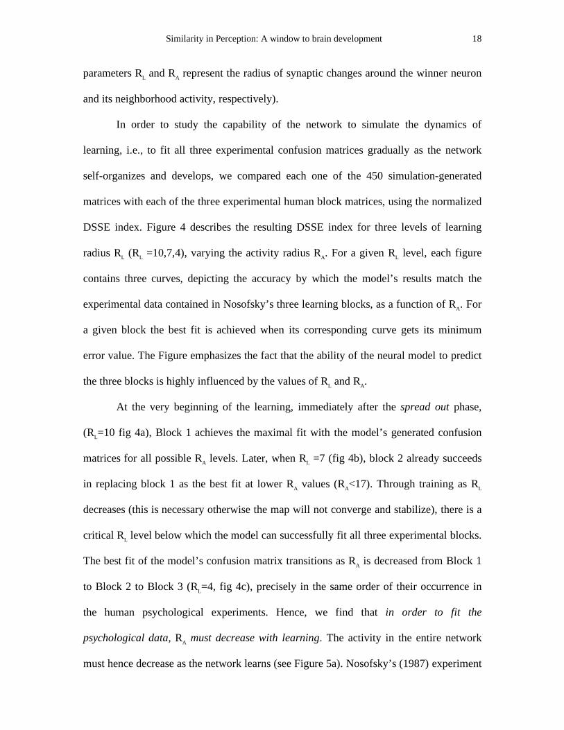
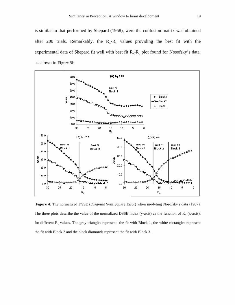
DSSE index. Figure 4 describes the resulting DSSE index for three levels of learning

radius RL (RL =10,7,4), varying the activity radius RA. For a given RL level, each figure

contains three curves, depicting the accuracy by which the model’s results match the

experimental data contained in Nosofsky’s three learning blocks, as a function of RA. For

a given block the best fit is achieved when its corresponding curve gets its minimum

error value. The Figure emphasizes the fact that the abilit y of the neural model to predict

the three blocks is highly influenced by the values of RL and RA.

At the very beginning of the learning, immediately after the spread out phase,

(RL=10 fig 4a), Block 1 achieves the maximal fit with the model’s generated confusion

matrices for all possible RA levels. Later, when RL =7 (fig 4b), block 2 already succeeds

in replacing block 1 as the best fit at lower RA values (RA<17). Through training as RL

decreases (this is necessary otherwise the map will not converge and stabili ze), there is a

critical RL level below which the model can successfully fit all three experimental blocks.

The best fit of the model’s confusion matrix transitions as RA is decreased from Block 1

to Block 2 to Block 3 (RL=4, fig 4c), precisely in the same order of their occurrence in

the human psychological experiments. Hence, we find that in order to fit the

psychological data, RA must decrease with learning. The activity in the entire network

must hence decrease as the network learns (see Figure 5a). Nosofsky’s (1987) experiment


is similar to that performed by Shepard (1958), were the confusion matrix was obtained

after 200 trials. Remarkably, the RA-RL values providing the best fit with the

experimental data of Shepard fit well with best fit RA-RL plot found for Nosofsky’s data,

as shown in Figure 5b.

Figure 4. The normalized DSSE (Diagonal Sum Square Error) when modeling Nosofsky's data (1987).

The three plots describe the value of the normalized DSSE index (y-axis) as the function of RA (x-axis),

for different RL values. The gray triangles represent the fit with Block 1, the white rectangles represent

the fit with Block 2 and the black diamonds represent the fit with Block 3.

�E��5/ �

��

��

��

��

��

��

��

��5$

'66(

%HVW�)LW%ORFN��


�F��5/ �

��

��

��

��

��

��

��5$

'66(




�D��5/ ��

��

��

��

��

��5$

'66(

%ORFN�%ORFN�%ORFN�



Figure 5. (a) Network activity during learning. The x-axis is the percentage of active neurons in the

network. A neuron is considered "active" when its activity passes a threshold value of 20% of the

winner's activity. The activity in the best fit networks decreases during training. (b) The best fit

combination of RA versus RL. The black diamonds represent the best fit combinations for the Nosofsky

(1987) experiment. The white square represents the best fit RA-RL combination for Shepard's (1958)

experiment.

Table 4 summarizes the simulation performance of the model in Nosofsky’s experiment

and compares it with two kinds of models. One is the classical multi -parametric MDS

choice model and the second is a version of the dynamic choice model simulated by

Nosofsky (1987). To reduce the number of parameters used, the simulation version of the

choice model performed by Nosofsky used the original feature coordinates in order to fit

the data with a bias free dynamic choice model. As evident in Table 4, the neural model

and the simulated dynamic choice model achieve similar levels of f it as measured by the

log-likelihood index.

��

��

��

%ORFN�� %ORFN�� %ORFN��

��RI�

DFWLY

H�QHX

URQV

�D�

��

�� 5/

5 $

1RVRIVN\�� 6KHSDUG��E�


Table 4. Performance during training on Nosofsky's dynamic 12 Munsell 's color experiment.

Model Correlation Sum SquareError

Log-LikelihoodRatio

Experiment FreeParameters

Nondiagonal

Total Diagonal(DSSE)

Total(SSE)

Nosofsky 1987

Block 1 Neural 2 0.78 0.74 0.95 1.4±0.5 4.7±0.8 -585±75

MDS

Dynamic

Choice

35 0.95 0.93 0.99 0.3 1.3 -386

Simulation of

Dynamic

Choice

2 -532

Block 2 Neural 2 0.86 0.72 0.98 0.9±0.4 4.2±0.7 -528±28

MDS

Choice

35 0.97 0.98 0.99 0.2 0.6 -268

Simulation of

Dynamic

Choice

2 -505

Block 3 Neural 2 0.83 0.77 0.99 0.9±0.3 2.5±0.4 -395±19

MDS

Choice

35 0.97 0.95 0.99 0.2 0.5 -235

Simulation of

Dynamic

Choice

2 -403

Understanding the model’s operation requires an investigation of the effect of training on

the network’s feature space. Figure 6 displays the spatial organization of the prototype

population vectors in the three network training states leading to maximal fit with Blocks

1, 2 and 3 respectively. The results demonstrate that representation of stimuli becomes

more discriminable over time, as the distances between the prototype population vectors

increases. Thus, the effect of the internal noise decreases (even though its absolute

magnitude remains fixed) and the identification performance gradually improves.


Figure 6. Spatial organization of the prototype population vectors during training. The figure depicts the

population encoding representations of the prototype vectors in the brightness/ saturation feature space

(solid squares). Time (training) progresses from subfigure (a) to (c).

Imposing Winner-Take-All (WTA) constraints on RA (by keeping RA constant and equal

to 1 through training) results in a severe degradation in the abilit y of the model to fit the

data (Figure 7). The WTA approach provides a good fit only towards the end of training

while at earlier stages its DSSE and SSE error indices are more than twice than those

achieved while optimally decreasing RA as a function of RL5.

5 It should be noted that RL and RA are not symmetric in the sense that RL is a crucial parameter for

network convergence and thus must gradually decrease over time. RA, in contrast, is significant only for

��

��

��

��

��

��

�� %ULJKWQHVV

6DWXU

DWLRQ

� ��

� � ��

��

5/ ��5$ ��E�

��

��

��

��

��

��

�� %ULJKWQHVV

6DWXU

DWLRQ

3URWRW\SH�9HFWRUV

� ��

�

� � ��

��

5/ ��5$ ��F�

��

��

��

��

��

��

��

� ��

��

� �� 6DWXU

DWLRQ

%ULJKWQHVV

�D� 5/ ��5$ ��


Figure 7. Quality of fit with fixed RA=1 (WTA constraint) versus optimal RA variation and population

coding simulating Nosofsky's experiment. The optimal RA variation and population coding is represented

by the gray bar, the WTA constraint is represented by a white bar. (a) The DSSE index (y-axis). (b) The

SSE index (y-axis). The standard error of the optimal RA-RL variation is portrayed by the error bar on top

of the gray bars.

DISCUSSION

In this study we have explored the abilit y of a neural model of similarity perception to

simulate five different indirect similarity experiments. Identifying a set of input stimuli

feature vectors, the model generates a confusion matrix that can be compared directly

with the pertaining experimental data. Our results suggest that self-organizing maps

based on the dynamics of population coding can model human responses fairly

accurately, using very few parameters. The principal findings suggest that in order to

obtain a good fit with the psychological data, the activity in the entire network must

"reading" the network's identification output, and its variation does not affect the organization of neural

map.

��

%ORFN� %ORFN� %ORFN�

'66(

2SWLPDO :7$�D�

��

%ORFN� %ORFN� %ORFN�

66(

2SWLPDO :7$�E�


gradually decrease while learning the task. Thus, the model predicts that simultaneously

with a gradual reduction in synaptic modifications, the network activity should also

gradually decline. To obtain a good fit one must use a population coding approach

instead of the perhaps more conventional WTA method for “ reading” the network’s

output. Finally, the model produces a reasonable fit to the experimental data of

3-dimensional perceptual space (Hodge 1962, See Table 3), where the SOM mapping to

the 2 dimensional network array also involves a reduction in the number of dimensions.

The topological organization and population coding characteristics of the neural

model find support in animal experiments of similarity as briefly reviewed in the

Introduction. Similar evidence for topographical maps has been recently found also in

higher perceptual levels (Fujita et al, 1992; Gochin et al, 1991; Wang et al., 1996;

Tanaka, 1996). The sparse population coding found in identification tasks involving a

long training period (e.g., Young & Yamane, 1992) fits with model’s prediction that the

activity should drop down as the map organizes.

The neural model presented here shares common fundamental properties with

previous psychological models. Like the GRT model, the neural model generates a new

representation of the stimuli i n the perceptual space. As in GRT, the identification of an

input stimulus depends on the boundaries in which the stimulus’ representation falls

in.The asymmetric relations are due to the asymmetric amounts of overlap between the

distributions corresponding to each class.. However, the GRT model relies on an explicit

ongoing supervised comparison between the stimuli and their representations in the

model to further adjust the model parameters to obtain maximal fit. In contrast, the

neural model achieves this maximization goal in a self-organizing unsupervised manner.

This property places our model in an ideal position to provide a natural, on line, account


of identification during training in neural terms. The neural model also shares common

computational principles with the MDS approach, since the topologically preserving

algorithm of the SOM well approximates the operation of a metric preserving algorithm

like MDS (Kaski, 1997). However, an important distinction between the operation of

our model and MDS-based choice models is that the output identification in the neural

model is performed in the original (possibly high-dimensional) feature space and not in

the reduced MDS space. In summary, the SOM-related neural model proposed here

provides an interesting example for a possible identification mechanism which

incorporates both GRT and MDS-like dynamics, suggesting that in some sense both these

approaches may play a part in similarity identification in the brain.

The main advantage of our model over previous MDS-choice and GRT models is

that it provides a neural level description for similarity perception in the brain. While

some of the earlier psychological mathematical models have obtained better fit with the

experimental data, the neural model obtains a fairly close fits to the data considering the

very few free parameters it uses. Furthermore, it should be emphasized that the number

of parameters embodied by the neural model is independent of the dimension and number

of stimuli . The model uses only two free parameters (RL, RA), given fixed values of

external and internal noise and guessing response, while previous psychological

mathematical models have required many free parameters since they rely on an explicit

representation of the distances between the stimuli and their biases. The neural model’s

parameters have a clear meaning in neural terms that helps us to better understand the

underlying physiological mechanisms. Since the model dynamics take place in a

self-organizing manner, stimulus identification is performed without the need to


explicitl y specify many parameters. Instead, the “distances” between stimuli are

implicitly defined by the geometry of the self-organized output feature space.

The biological plausibilit y of the population coding method and the

Self-Organizing Map algorithm has been argued by Georgopoulos et al. (1982, 1984)

and Kohonen (1993), respectively. The population coding method has been found to

provide a fair account of neural activity pattern, during variety tasks and different

modaliti es (e.g., Georgopoulos et al., 1989, Schwartz, 1994). The Winner-Take-All

function can be implemented by laterally connected network with excitatory short range

lateral feedback connections and inhibitory longer range ones. Under these conditions a

“peak” of activity is formed at the neural cluster that best matches the external input.

The learning procedure can be implemented by synaptic interactions that are mediated

via a diffuse chemical agent (grossly represented in our model by the RL parameter).

During learning the effective range of the diffuse chemical modulation is decreased from

a fairly wide to a narrow value. A good candidate for the diffuse neuromodulator agent

may be Nitric Oxide (NO) that has been found to be produced in proportion to the

postsynaptic potential and to control synaptic plasticity (Fazeli , 1992). The neighborhood

activity around the winner neuron can be controlled by an inhibitory process which is

represented by the RA parameter and mainly reflects the activation of the long range

inhibitory connections. The realization of such a decrease in the radius of activation

surrounding winning neurons may occur in biological networks via the action of second

order processes such as neural fatigue and adaptation. The main motivation for assigning

distinct parameters for RL and RA was that synaptic modifications and neural activity

might be governed by different modulation processes such as distinct neuromodulators


and diffuse chemicals. Nevertheless, the finding that these two processes covary in the

same direction supports the possibilit y that one can obtain successful SOM models of

similarity perception using activity-dependent Hebbian learning without the need to

specify an explicit radius of learning.

In summary, this paper presents a novel neural model of identification, forming a

tentative conceptual bridge between the pertaining psychological and neurophysiological

data. The need to fit the cognitive experimental data, in turn, suggests interesting

constraints concerning brain organization and development in perceptual processing

regions.

Acknowledgments

We thank Daniel Algom for his helpful comments and suggestions. Reprints requests

should be sent to Eytan Ruppin Departments of Computer Science & Physiology,

Tel-Aviv University, Tel-Aviv 69978, Israel, or via e-mail: [email protected] .

References

Ashby, F. G., & Perrin, N. A. (1988). Toward a unified theory of similarity and

recognition. Psychological Review, 95, 124-150.

Ashby, F. G., & Townsend, J. T. (1986). Varieties of perceptual independence.

Psychological Review, 93, 154-179.

Ashby, F. G., & Lee, W. W. (1991). Predicting similarity and categorization from

identification. Journal of Experimental. Psychology: General, 120, 150-172.


Edelman, S. (1995). Representation of similarity in 3D object discrimination. Neural

Computation, 7, 407-422.

Edelman, S., & Duvdevani-Bar, S. (1997). Similarity, connectionism and the problem of

representation in vision. Neural Computation, 9, 701-720.

Fujita, I., Tanaka, K., Ito, M., & Cheng, K. (1992). Columns for visual features of

objects in monkey inferotemporal cortex. Nature, 360, 343-346.

Georgopoulos, A. P., Kalaska, J. F., Caminiti , R., & Massey, J. T. (1982). On the

relations between the direction of two-dimensional arm movements and cell discharge

in primate motor cortex. Journal of Neuroscience, 2, 1527-1537.

Georgopoulos, A. P., Kalaska, J. F., Crutcher, M. D., Caminiti , R., & Massey, J. T.

(1984). The representation of movement direction in the motor cortex: Single cell and

population studies. In Edelman, G. M., Gall , W. E, &. Cowan, W. M, (Eds.). Dynamic

aspects of neocortex.

Georgopoulos, A. P., Lurito, J. T., Petrides, M., Schwartz, A. B., and Massey, J. T.

(1989). Mental rotation of the neural population vector. Science, 243, 234-236.

Gochin, P. M., Mill er, E. K., Gross, C. G., & Gerstein, G.L. (1991). Functional

interactions among neurons in inferior temporal cortex of the awake macaque.

Experimental Brain Research. 84, 505-516.

Grajski, K., & Merzenich, M. (1990). Hebb-type dynamics is suff icient to account for the

inverse magnification rule in cortical somatotopy. Neural Computation. 2, 71-84.

Guenther F. H., & Gjaja M. N. (1996). The perceptual magnet effect as an emergent

property of neural map formation. Journal of the Acoustical Society of America, 100,

1111-1130.


Hodge, M. H. (1962). Confusion matrix analysis of single and multidimensional auditory

displays. Journal of Experimental Psychology, 63, 129-142.

Kaski, S. (1997). Data Exploration using self-organizing maps. Mathematics and

Management in Engineering No. 82, Acta Polytechnica Scandinavica, Finnish

Academy of Technology.

Kent, F. K., Youngentob, S. L., & Paul R. S. (1995). Odorant-specific spatial patterns in

mucosal activity predict perceptual differences among odorants. Journal of

Neurophysiology, 74, 1777-1781.

Kohonen, T. (1982). Self-organized formation of topologically correct feature maps.

Biological Cybernetics, 43, 59-69.

Kohonen, T. (1989). Self-Organizing and Associative Memory. (3rd ed.) Springer,

Berlin.

Kohonen, T. (1993). Physiological interpretation of the self-organizing map algorithm.

Neural Networks, 6, 895-905.

Kornbrot, D. E. (1978). Theoretical and empirical comparison of Luce’s choice model

and logistic Thurstone model of categorical judgment. Perception & Psychophysics,

24, 193-208.

Kuhl, P.K. (1991). Human adults and human infants show a ‘perceptual magnet effect’

for the prototypes of speech categories, monkeys do not. Perception & Psychophysics,

50, 93-107.

Luce, R. D. (1963). Detection and recognition. In Handbook of mathematical

psychology, Luce, R. D., Bush, R.R., Galanter, E. (Eds.). 1, 103-190. New York:

Wiley.


Nakatani, L.H. (1972). Confusion-choice model for multidimensional psychophysics.

Journal of Mathematical Psychology, 9, 104-127.

Nosofsky, R. M. (1985). Luce's choice model and Thurstone's categorical judgment

model compared: Kornbrot's data revisited. Perception & Psychophysics, 37, 89-91.

Nosofsky, R.M. (1987). Attention and learning processes in the identification and

categorization of integral stimuli . Journal of Experimental Psychology: Learning

Memory & Cognition, 13, 87-109.

Nosofsky, R. M. (1989). Further tests of an exemplar-similarity approach to relating

identification and categorization. Perception & Psychophysics, 45, 279-290.

Nosofsky, R. M. (1992). Similarity Scaling And Cognitive Process Models. Annual

Review of Psychology, 43, 25-53.

Schwartz, A. B. (1994). Direct cortical representation of drawing. Science, 265, pp.

540-542.

Shepard, R. N. (1957). Stimulus and response generalization: A stochastic model relating

generalization to distance in psychological space. Psychometrika, 22, 325-345.

Shepard, R.N. (1958). Stimulus and response generalization: Tests of a model relating

generalization to distance in psychological space. Journal of Experimental

Psychology, 55, 509-523.

Tadashi, S., Edelman, S., & Tanaka, K. (1998). Representation of objective similarity

among three-dimensional shapes in the monkey. Biological Cybernetics, 78, 1-7.

Tanaka, K. (1996). Inferotemporal cortex and object vision. Annual Review of

Neuroscience, 19,109-139.

Wang, G., Tanaka, K., & Tanifuji , M. (1996). Optical imaging of functional

organization in the monkey inferotemporal cortex. Science, 272, 1665-1668.


Wickens, T.D. (1982). Models for behavior: Stochastic processes in psychology. San

Francisco: Freeman.

Young M. P., & Yamane S. (1992). Sparse population coding of faces in the

inferotemporal cortex. Science, 256, 1327-1331.

Youngentob, S.L., Markert, L.M., Mozell , M.M., & Hornung, D.E. (1990). A method for

establishing a five odorant identification confusion matrix task in rats. Physiology &

Behavior, 47, 1053-1059.

Appendix I - Normalization of input feature stimuli vectors.

In order to normalize the input feature vectors, an agonist-antagonist method was used in

the simulations (Guenther & Gjaja, 1996). This method replaces each feature input

component L[ with a new agonist-antagonist input of the form

(1)( ) ( )��

LL0$;L0,1L

L0,1LL [[[[

[[[−+−

−=+

(2)( ) ( )��

LL0$;L0,1L

LL0$;L [[[[

[[[−+−

−=−

where the index i indicates the feature dimension number, L[ is the value of the feature

component i in input vector x, and +L[ and −

L[ are the new agonist-antagonist

representations receptively of feature component i. The constants L0$;[ and L0,1[ are the

maximum and minimum values, respectively, for the i th feature component.


Appendix II - Euclidean distance calculations.

The Euclidean distance d between the output vector and the prototype population vector

p is calculated by

(3)( )∑ −

−= N

N0,1N0$;

SNN

[[[[G �

�

�� ,

where N[ is the k component of the input vector x and SN[ is the kth component of the

prototype population vector p. N0$;[ and N0,1[ are the maximum and minimum values,

respectively, for the kth feature component.

Appendix III - Log-Likelihood Ratio Testing.

The log-likelihood ratio testing is used to determine the quality of f it between the

psychological data and the prediction of the neural model (Wickens 1982):

(4) ∑ ∑∑ ∑∑ ⋅+−= L M LMLML M LML L SII1/ OQ�OQ�OQOQ ,

where Ni is the frequency with which stimulus i was presented, f ij is the observed

frequency with which stimulus i was identified as stimulus j, and pij is the predicted

probabilit y with which stimulus i is identified as stimulus j.

Date post:	14-Apr-2018
Category:	Documents
Upload:	buituong
View:	216 times
Download:	3 times

Similarity in Perception: A W indow to Brain …ruppin/similarity.pdfSimilarity in Perception: A W...

Documents