Page 1
i
Similarity Tests for Metamorphic Virus Detection
A Project Report
Presented to
The Faculty of the Department of Computer Science
San Jose State University
In Partial Fulfillment
of the Requirements for the Degree
Master of Computer Science
by
Mahim Patel
May 2011
Page 2
ii
© 2011
Mahim Patel
ALL RIGHTS RESERVED
Page 3
iii
SAN JOSÉ STATE UNIVERSITY
The Undersigned Project Committee Approves the Project Titled
Similarity Tests for Metamorphic Virus Detection
by
Mahim Patel
Approved for the Department of Computer Science
___________________________________________________________
Dr. Mark Stamp, Department of Computer Science Date
___________________________________________________________
Dr. Chris Pollett, Department of Computer Science Date
___________________________________________________________
Dr. Soon Tee Teoh, Department of Computer Science Date
Approved for the University
___________________________________________________________
Associate Dean Office of Graduate Studies and Research Date
ABSTRACT
Page 4
iv
Similarity Tests for Metamorphic Virus Detection
by Mahim Patel
A metamorphic computer virus generates copies of itself using code morphing techniques. A
new virus has the same functionality as the parent but it has a different internal structure. The
goal of the metamorphic virus writer is to produce viral copies that have no common signature. If
the viral copies are sufficiently different, they can evade signature detection, which is the most
widely-used anti-virus technique.
In previous research, hidden Markov models (HMMs) have been used to detect some
metamorphic viruses. However, recent research has shown that it is possible for carefully
designed metamorphic viruses to evade HMM-based detection.
In this project, we analyze similarity-based techniques for detecting metamorphic viruses. We
first consider a similarity index technique that was previously studied. We then consider new
similarity techniques based on edit distance and pairwise sequence alignment. We test these
similarity measures on the challenging problem of metamorphic virus detection. We compare our
detection results with those obtained using an HMM-based detection method.
Page 5
v
ACKNOWLEDGEMENTS
I would like to express my deep and sincere gratitude to my project advisor, Dr. Mark Stamp for
his guidance, encouragement, and support throughout the project.
Page 6
vi
TABLE OF CONTENTS
1. INTRODUCTION .............................................................................................................1
2. COMPUTER VIRUS ........................................................................................................2
3. VIRUS PREVENTION TECHNIQUES ...........................................................................3
3.1 SIGNATURE DETECTION ....................................................................................................3
3.2 HEURISTIC ANALYSIS .......................................................................................................4
4 VIRUS EVOLUTION .......................................................................................................4
4.1 ENCRYPTED VIRUSES .......................................................................................................4
4.2 POLYMORPHIC VIRUSES ....................................................................................................5
4.3 METAMORPHIC VIRUSES ...................................................................................................6
4.3.1 Register Swap (Register Usage Exchange) ...............................................................6
4.3.2 Junk Instruction Insertion ........................................................................................7
4.3.3 Equivalent Instruction Substitution ..........................................................................8
4.3.4 Instruction Transposition .........................................................................................8
4.3.5 Subroutine Transposition .........................................................................................9
5 SIMILARITY-BASED TECHNIQUES ......................................................................... 10
5.1 SIMILARITY INDEX TEST METHOD .................................................................................. 10
5.2 EDIT DISTANCE .............................................................................................................. 13
5.2.1 Computing Edit Distance ....................................................................................... 13
5.2.2 Edit Distance for Op-code Sequences..................................................................... 15
5.3 PAIRWISE SEQUENCE ALIGNMENT METHOD .................................................................... 16
5.3.2 Op-code Conversion .............................................................................................. 17
5.3.3 Pairwise Alignment Scoring ................................................................................... 18
5.3.4 Substitution Matrices and Gap Penalties ................................................................ 18
5.3.5 Scoring Pairwise Op-code Sequence Alignment ..................................................... 22
6 EXPERIMENTS AND RESULTS .................................................................................. 22
6.1 SIMILARITY INDEX ......................................................................................................... 22
6.1.1 Base Virus ............................................................................................................. 22
6.1.2 Morphed Virus ....................................................................................................... 26
6.1.3 Similarity Among Same Family Viruses.................................................................. 28
6.1.4 Morphed Virus Detection using a Default Window Size.......................................... 29
6.1.5 Morphed Virus Detection by Varying Window size ................................................. 31
6.2 EDIT DISTANCE .............................................................................................................. 37
6.3 PAIRWISE SEQUENCE ALIGNMENT................................................................................... 40
Page 7
vii
6.3.1 Base Virus and Non-Virus Op-code Sequence Alignment ....................................... 40
6.3.2 Morphed Virus and Non Virus Op-code Sequence Alignment ................................. 41
7 CONCLUSION ................................................................................................................ 45
8 FUTURE WORK ............................................................................................................ 46
9 REFERENCES ................................................................................................................ 47
Page 8
viii
LIST OF FIGURES
Figure 1 Pseudo Code of Virus and Infect Module [8] .................................................................3
Figure 2 Polymorphic Virus Generations [18] .............................................................................5
Figure 3 Metamorphic Virus Generations [18] ............................................................................6
Figure 4 Two different generations of RegSwap [9] ....................................................................7
Figure 5 Dead Code Insertion in Evol Virus [14] .........................................................................8
Figure 6 Subroutine Transposition ...............................................................................................9
Figure 7 Similarity between two Assembly Programs ................................................................ 12
Figure 8 Pseudo code for Levenshtein Distance [23] ................................................................. 14
Figure 9 Edit Distance between String s1 and s2 ....................................................................... 15
Figure 10 Op-code to Symbol Lookup Mapping [26] ................................................................ 17
Figure 11 Alignment of two Op-code Sequences from NGVCK Virus [26] ............................... 18
Figure 12 The Table for AGGTTGC and AGGTC [28] ............................................................. 19
Figure 13 Substitution Matrix for Op-codes with Values for Relative Scores ............................. 19
Figure 14 Similarity Scores between Normal Files and between Virus and Normal files............ 24
Figure 15 Graph of File Size and different Percentage of Junk Code Insertion ........................... 28
Figure 16 Similarity Graph of Scores for Base Viruses, and Morphed Viruses........................... 29
Figure 17 Similarity Graph for Morphed Viruses and Normal Files ........................................... 30
Figure 18 Similarity Graph of Scores for different Window Size ............................................... 34
Figure 19 Graph of Error Rate for different Window Size ......................................................... 37
Figure 20 Similarity Graph for Morphed Viruses and Normal Files ........................................... 38
Figure 21 Graph of Error Rates for Various Morphed Virus Copies........................................... 40
Figure 22 Alignment Scores for Non-Virus and Virus Op-code Sequences ................................ 41
Figure 23 Alignment Scores for Non-Virus, and Various Morphed Virus Op-code Sequences... 43
Page 9
ix
Figure 24 Graph of Error Rates for Various Morphed Virus Copies........................................... 44
Figure 25 Graph of Error Rates produced by different Similarity-Based Methods...................... 45
Page 10
x
LIST OF TABLES
Table 1 W32.MetaPhor Instruction Substitution [15] ...................................................................8
Table 2 File Op-code Sequences ............................................................................................... 11
Table 3 Op-code to Symbol Conversion .................................................................................... 16
Table 4 Similarity Scores between Virus and Normal Files, and between Normal Files. ............ 24
Table 5 Similarity Graphs for Two Chosen Virus Pair and One Normal File Pair ...................... 26
Table 6 Similarity Graphs between the Morphed Virus and the Normal File.............................. 27
Table 7 Error Rate for Morphed Viruses having Window Size of 5 ........................................... 31
Table 8 Similarity Scores between Normal Files for different Window Size .............................. 32
Table 9 Similarity Score of Files having different Window Size ................................................ 36
Table 10 Similarity Scores for Various Programs using Edit Distance Technique ...................... 39
Table 11 Sequence Alignment Scores between Various Programs ............................................. 41
Page 11
1
1. INTRODUCTION
A computer virus is a program that, when executed, replicates itself without the user‟s
permission or knowledge [13]. A virus spreads its infection by attaching itself to other
executable code. The infected program, when launched, can then replicate itself to infect other
executables and change their behavior [8]. Note that a virus relies in some way on other
executable code to spread its infection.
A virus might perform malicious activities such as corrupting the file system by infecting batch
files, macros, shell script, system sectors, companion and binary executable. Modern viruses also
called worms take advantage of the Internet to propagate over the network and spread their
infection globally.
Virus construction kits are available, which makes virus creation extremely simple [19].
Consequently, users who have minimal knowledge can create potential viruses. There are several
antivirus programs available that can be used to detect malware [16]. The most commonly used
antivirus detection technique is signature detection, which consists of searching the content of
the files in file for “signatures” stored in antivirus database. A signature consists of a string of
bits found in a particular virus. Another detection approach is code emulation, where code is
executed in a virtual environment and its actions are recorded in log file. Based on logged action,
the antivirus determines whether the program is a virus or not [16].
To evade signature-based detection, virus writers sometimes use code obfuscation techniques
which alter the structure of the code. The techniques used to obfuscate code include reordering
assembly instructions, dead code insertion, and equivalent instruction substitution [3]. The result
is a morphed virus that has the same functionality as the original. However, if the morphing is
sufficient, no common signature will exist. These metamorphic viruses generate different copies
of it using code morphing techniques.
To contend with metamorphic viruses, a detection tool based on hidden Markov models (HMMs)
was developed [2]. This virus detection tool is initially trained on metamorphic variants
belonging to the same family. Then the trained model can be used to detect new metamorphic
variants from the same family. This technique was successful at detecting all hacker-generated
metamorphic viruses tested [2]. Several of the metamorphic viruses studied in [2] were not
Page 12
2
detected by commercial virus scanners. Subsequent work has shown that it is possible to produce
a metamorphic generator that can evade signature detection and HMM-based detection [3].
The goal of the research presented here is to test similarity-based approaches to see if we can
detect the metamorphic viruses in [3]. Similarity index techniques classify a program as belong
to virus family provided that it is sufficiently similar to a given member of the family.
This paper is organized as follows. Section 2 contains background information on computer
viruses. In Section 3, we discuss antivirus techniques. Then in Section 4, we detail various code
obfuscation techniques that can be used to generate highly morphed viruses. Section 5 presents
the design and implementation of our several similarity-based techniques. Section 6 covers
experimental results obtained from our similarity-based method experiments involving
metamorphic viruses. Section 7 presents our conclusions. Finally, Section 8 presents possible
future work.
2. COMPUTER VIRUS
Computer virus is self-replicating program that performs malicious activities by infecting other
host files. The host files, when executed, can infect other files in turn. For example, the file
infector virus, which embeds itself in the code of other host programs. The infected file can be
any executable application. On execution of the infected program, virus loads itself into the
computer‟s memory and continues to run even after the host files shut down its execution.
“Before the initiation of the internet, file infector viruses accounted for probably 85% of all virus
infections [11].”
A typical virus comprises of three modules [8] which are infect, trigger and payload. The method
infect defines the process of spreading viruses by changing the host to contain a copy of the virus
code. Trigger is a test condition, which decides to load payload or not. Payload defines the
damage by the virus. Figure 2 shows the pseudo code which will infect the target.
Page 13
3
Figure 1 Pseudo Code of Virus and Infect Module [8]
3. VIRUS PREVENTION TECHNIQUES
This section outlines some of the most commonly used techniques to detect computer viruses.
3.1 Signature Detection
Signature detection technique is widely used to detect viruses. Signature is a pattern of bits found
in a virus [1]. These string of bits, which are found in a virus file are stored in the antivirus
databases. The virus scanner searches the entire file system for known signatures. If the known
signature is found then the file is marked as infected. For example, executable file infected by
“W32.Sample.A” virus comprises of the following pattern of bits as signature [12].
The virus scanner searches the entire file system for this signature and if found, it declares the
file to be the Beast virus.
Page 14
4
Some virus scanners support wildcard search strings, such as “??02 34C9 8CD1 429C” where „?‟
indicates the wildcard. These wildcard strings permit skipped bytes and regular expressions,
which also helps in detecting encrypted viruses in some cases [17].
3.2 Heuristic Analysis
Heuristic analysis is a method used by the antivirus software‟s to detect new or unknown
computer viruses. There are two types of heuristic scanning techniques. The difference between
the two approaches is whether the heuristic scanner makes use of CPU emulation to scan for
virus like behavior or not. A heuristic scanner has two phases of operation when scanning files
for viruses. In the first phase of the operation, the scanner observes the behavior of the program
and looks for a specific area in the file where the virus would attach itself. In the second phase, it
determines the program logic which can be executed by computer instructions in the specific
areas identified in the first phase [10]. The program is flagged as a virus, if it contains a certain
percentage of the computer instructions similar to the viral instructions.
The Heuristic analysis results in many false positives as it mostly operates on the basis of past
experience [20]. This might not detect new viruses that contain code different from a previously
known virus program. The heuristic scanner creates many false positives which can lose users‟
trust and interest.
4 VIRUS EVOLUTION
The following techniques are different strategies used by virus writers to make their viruses more
difficult to detect.
4.1 Encrypted Viruses
Encryption is the simplest way to conceal a virus from the antivirus program. The encrypted
virus contains an encrypted body and a decryptor module. Most of the antivirus programs
attempt to find the virus by looking for a specific string of bits in a program. To avoid detection,
viruses encrypt the body using the encryption key to conceal the pattern of code. Different
encryption key generates a different encrypted virus body. The logic of encryption is kept
simple, such as XOR, the key for encrypting the virus body [3]. The encrypted virus body is
Page 15
5
different in all infections, but the decryptor module is similar in all infected copies. The antivirus
program can detect the decryptor by its code pattern even if it cannot decrypt the virus body.
4.2 Polymorphic Viruses
Polymorphic viruses are one of the more complex techniques implemented by virus coders to
overcome the disadvantage of the encrypted viruses [19]. To make it more effective than the
encrypted viruses, polymorphic viruses have different methods of decryption by mutating the
decryptor logic. More advanced versions of the polymorphic virus substitutes the mutually
independent instructions, such as moving “0” to B or adding “0” to A, resulting in inexact
values. This evades the antivirus program looking for a specific code of pattern in the virus [16].
To detect polymorphic viruses, virus scanners based on signature detection method have to
search different string of bits for each likely decryption methods.
Anti-virus software even uses code emulation to detect the polymorphic virus. The code
emulator lets the virus execute and observe its behavior. It emulates the decryption process and
detects the decrypted virus body.
Figure 2 Polymorphic Virus Generations [18]
Page 16
6
4.3 Metamorphic Viruses
Virus writers have developed metamorphic viruses which do not carry any decryptor or constant
virus body like polymorphic viruses. A metamorphic virus changes its code at each infection by
using various code obfuscation techniques. Code obfuscation techniques are performed on both
the data section and the control flow of an assembly program [15]. Control flow obfuscation
technique involves unconditional jump instructions and instruction reordering. Data flow
obfuscation is achieved by transposition, junk code insertion, equivalent instruction substitution,
register renaming, and subroutine permutation. This makes it more resistant to code emulation
detection technique. Unlike polymorphic viruses, encryption is not used in metamorphic viruses.
The virus body has different structures with same functional behavior. Figure 3 shows a
metamorphic virus with different body structures.
Figure 3 Metamorphic Virus Generations [18]
4.3.1 Register Swap (Register Usage Exchange)
Register swapping is one of the simplest metamorphic techniques. This technique changes
register operands in the virus body with different equivalent registers. Instructions remains
Page 17
7
constant for all virus generation, only register changes. For example, instruction “mov edi,
0004h” can be substituted with “mov ebx, 0004h.” The W95/RegSwap virus [7] is an example of
metamorphic virus that uses the register swap technique. Figure 4 shows a sample code snippet
from RegSwap, which follows register swapping technique. Wildcard string can usually detect
such metamorphic viruses [17].
Figure 4 Two Different Generations of RegSwap [9]
4.3.2 Junk Instruction Insertion
Junk code insertion is an effective technique employed by metamorphic viruses to change the
appearance of the virus body. Junk instructions do not have an effect on the program outcome
and it may not even execute [13]. Examples of do-nothing instructions are “mov edx, edx”, “add
R1, 0”, “sub R1, 0” or “nop.”
Dead code insertion can be done as a single instruction or a block of instructions between the
core instructions. Figure 5 shows the example of the Evol virus which implemented the junk
code insertion technique by adding a block of dead code.
Page 18
8
Figure 5 Dead Code Insertion in Evol Virus [14]
4.3.3 Equivalent Instruction Substitution
Equivalent instruction substitution is another useful technique used to substitute an instruction or
a block of instructions with an equivalent instruction or an equivalent block of instructions. For
example, “push edx,” “pop eax” can be substituted by “add eax,1” followed by “mov eax,edx.”
Table 1 shows the W32/MetaPhor virus [15] implementing instruction substitution. The “mov
reg,imm” operation is equivalent to “mov mem,reg” followed by “op mem,reg2” and “mov
reg,mem.”
Table 1 W32.MetaPhor Instruction Substitution [15]
4.3.4 Instruction Transposition
Transposition is a method to change the order of execution of the instructions. Instruction
permutation between the instructions does not affect the program outcome and it can be applied
only if there is no mutual dependency between the instructions. Consider the following
instruction set:
(op1 r1, r2)
(op2 r3, r4) // r1 and/or r3 register are to be modified
Page 19
9
The instructions can be reordered only if following conditions are satisfied:
i) r1 is not equal to r4,
ii) r2 is not equal to r3,
iii) r1 is not equal to r3,
For example, instructions “mov edx,eax” and “add ecx,3” can be swapped as they satisfy the
transpose criteria.
… …
mov edx,eax add ecx,3
add ecx,3 mov edx,eax
4.3.5 Subroutine Transposition
Subroutine transposition is an effective technique that changes the appearance of a virus by
reordering the subroutines. There can be n! different generation of subroutines for n different
subroutines. The W32/Ghost virus [15] implements the subroutine transposition technique. This
virus contains 10 subroutines generating 10! distinct copies. Detection of such virus can be
accomplished by the string driven pattern detection technique.
Figure 6 Subroutine Transposition
Page 20
10
5 SIMILARITY-BASED TECHNIQUES
To evade the signature based detection and HMM-based detection, the metamorphic generator
produces highly morphed copies of itself [3]. Each generation of viruses is different in structure.
We consider different similarity-based approaches to see if we can detect the highly morphed
viruses [3]. The similarity-based methods measure the similarity between the dissimilar virus
copies. It classifies a program as belonging to a virus family or non-virus family based on the
similarity results obtained by comparisons between several virus and non-virus programs;
between virus programs; and between non-virus programs. We first considered a similarity index
technique that was previously studied [4]. We then considered new similarity techniques based
on edit distance and pairwise sequence alignment methods.
5.1 Similarity Index Test Method
To measure the similarity between the virus copies, two assembly files are compared based on
the op-code sequence presented in them. The following steps are followed to compute the
similarity between two files and are graphically illustrated in Figure 7.
1. Given two assembly files, file1.asm and file2.asm, we extract the sequence of op-codes
from both the files, excluding labels, comments, blank lines and other directives. Let‟s
call these resulting op-code sequences F1 and F2 for file1.asm and file2.asm,
respectively. Let m and n represent the number of op-codes in F1 and F2, respectively. A
number is assigned to each of the op-code in the resulting op-code sequence: 1 for the
first op-code, 2 for the second, and so on.
2. Op-code sequence is divided into subsequences of three consecutive op-codes as shown
in Figure 8. We compare the op-code sequences, F1 and F2, considering all the
subsequences of three consecutive op-codes from each sequence. We considered a match,
if three op-codes are the same in any order. For example F1 is (add, call, test, sub, mov)
and F2 is (mov, add, call, sub, test). The sequence (call, test, sub) in F1 matches with
(call, sub, test) of F2. The process is repeated for all the op-codes in F1 and F2.
For example:
Opcode Op-code sequence
Page 21
11
Index F1 F2
0
1
2
3
4
add
call
test
sub
mov
mov
add
call
sub
test
Table 2 File Op-code Sequences
3. As shown in Figure 7, m and n represents total number of op-code in F1 and F2
respectively. To find the total number of matches in F1, all matches are computed and
added together. The total number of match is divided by m to get the similarity score of
F1. Similarly, similarity score for F2 is computed.
Similarity score for F1: S1= (total number of matches in F1) / m
Similarity score for F2: S2= (total number of matches in F2) / n
4. The similarity score between the files, file1.asm and file2.asm is obtained by taking the
average of F1 and F2.
Total Similarity Score: (S1+S2)/2
Page 22
12
Figure 7 Similarity between Two Assembly Programs
A graph is generated to show the similarity of the assembly files. The following steps are
followed to generate the graph:
1 We mark the match on the graph coordinate(X,Y) where X represents the op-code number of
the first op-code of the three op-code subsequence in file F1, and Y represents the op-code
number of the op-code subsequence in file F2.
2 A graph can plot a grid of dimension n × m to visualize the similarity of both files by
marking all the matched coordinates. The x-axis represents the op-code numbers of file F1
and the y-axis represents the op-code numbers of file F2.
3 The graph in Figure 7 is very populated with the matches. This makes it difficult to
understand the similarity. So to remove noise and to make similarity index technique more
efficient, we determine a window size (i.e. threshold). The similarity score match below the
window size is dropped. In Figure 7, the window size forms the line segments having the
length greater than 5.
Page 23
13
5.2 Edit Distance
Levenshtein distance (i.e. an edit distance) is an algorithm to measure the number of edit
operations needed to transform one string into another [23]. For given string s1 and s2, the edit
distance is calculated based on the amount of difference between the two sequences of the
strings. The difference in the strings is based on the sequence of characters each string contains.
Allowable edit operation to transform one into another are insertion, deletion and substitution.
For example, the edit distance between “meeting” and “readings” is 4, as the following four edits
are required to change one string into the other, and there is no alternate way to get the same
result in fewer than four edits [23]:
1. meeting → reeting (substitution of „r‟ for „m‟)
2. reeting →reating (substitution of „a‟ for „e‟)
3. reating → reading (substitution of „d‟ for „t‟)
4. reading → readings (insertion of „s‟ at the end)
5.2.1 Computing Edit Distance
For a given two sequence s1 and s2 and three edit operations, the edit distance for the sequences
is valued to transform sequence s1 to sequence s2. We use dynamic programming to find the edit
distance from s1 to s2.
If s1 has n characters and s2 has m characters, D(i,j) is the least distance between the first i
characters of s1 and the first j characters of s2. So the edit distance between s1 and s2 is given by
D(n,m) .
D(i,0) = i , as i deletions are required to transform a string with i characters to the empty string
D(0,j) = j, as j insertions are required to transform an empty string into a j character string
In general
D(i,j) = min {[D(i-1,j)+1], [D(i,j-1)+1], [D(i-1,j-1)+ (0, if s1[i])=s2[j] or 1, if s1[i] != s2[j]) ] }
The psuedocode is pointed directly ahead as shown in Figure 8.
Page 24
14
Figure 8 Pseudo code for Levenshtein Distance [23]
We can draw an (n+1)*(m+1) matrix, following the pseudocode by filling it, top to bottom, left
to right. The initial row and column can be filled as mentioned above, proceeding row by row to
fill the remaning entries in the matrix. The matrix shown in Figure 9, gives the edit distance
between MEETING and READINGS. The total entries in the matrix is O(mn) and each
computation takes O(1) constant time. The total running time is O(mn).
Page 25
15
Figure 9 Edit Distance between String s1 and s2
5.2.2 Edit Distance for Op-code Sequences
To find similarity between two virus files, all the op-codes from each assembly file were
extracted and the comparison between the op-codes present in both the virus files were done. The
edit distance technique deals with the sequence of the characters and finds the edit score. To use
the edit distance technique for finding the similarity between virus copies, we assigned unique
symbols to each op-code. For scoring edit distance, we have only considered the op-codes that
appear in the Table 3.
OP-
CODE
SYMBOL OP-
CODE
SYMBOL
xchg a lea v
jmp b popad w
mov c pushad x
adc d pop y
add e push z
and f jnz A
cmp g jz B
sbb h nop C
sub i rep D
xor j retn E
div k ret F
Page 26
16
Table 3 Op-code to Symbol Conversion
The following steps are followed to compute the similarity between two files:
1. Given two assembly files, file1.asm and file2.asm, op-code sequence are extracted from
both the files as described in Section 5.1. Let‟s give names to the resulting op-code
sequence from file1.asm and file2.asm as F1 and F2.
2. Replace each op-code with their respective symbol as shown in Table 3. As a result, the
sequence of symbols F1 and F2 is formed from sequence of op-codes F1 and F2.
3. The above steps allow the edit distance technique to calculate the number of edit
operations required to convert the sequence of symbols from F1 to F2. The length, x and
y is number of symbols in F1 and F2 respectively. ed(x,y) is the edit distance score for F1
and F2.
4. Similarity between two programs of length x and y respectively is:
[1 - ed(x, y) / max(x, y)]
5.3 Pairwise Sequence Alignment Method
The sequence alignment is a method which arranges different sequences of DNA, or protein to
determine the region of similarity due to structural, or functional relationships between the
mul l movzx 1
neg m movsd 2
not n movsb 3
shl o stosb 4
shr p stosd 5
test q Lodsb 6
inc r Lodsd 7
call s invoke 8
dec t stdcall 9
or u
Page 27
17
sequences. Aligned sequences of nucleotide or amino acid are represented as rows in matrix, and
symbols as individual columns [25].
5.3.2 Op-code Conversion
A disassembled virus program is sequence of op-codes. Previous studies in [26] have showed
that instead of considering all the instructions, only 36 high level op-code instructions are taken
into account while aligning pairs of op-code sequences. The most frequently used op-codes will
be considered and each of them is assigned with a single character as a symbol. The symbols are
the letters from the English alphabet and single numerical digits. The rest of the op-codes are
assigned with an asterisk „*‟ [26].
By this approach, less number of unique op-codes are aligned in an op-code sequence. The top
14 op-codes account for approximately 90% of all the instructions used in any typical program
[27]. In this research, the 36 most frequently used op-codes accounted for approximately 99.3%
of all op-codes found in sequences [26].
Figure 10 Op-code to Symbol Lookup Mapping [26]
Page 28
18
The representation of unique op-codes and their symbols is shown in Figure 10. The op-codes
are shown by the frequency, where op-code „mov‟ assigned with symbol „A‟ is most frequent
and least frequent op-code „sbb‟ with symbol „9‟ [26]. The op-codes with the asterisk „*‟ symbol
rarely appears.
5.3.3 Pairwise Alignment Scoring
The op-code conversion is done as described in Section 5.3.1. To detect the metamorphic
viruses, a proper alignment approach needs to be defined. For the same pair of sequences, no
alignment is required. In pairwise alignment, sequences are represented as rows in matrix, and
symbols as individual columns. All the symbols in sequence 1 are aligned with the symbols in
sequence 2 to get related symbols aligned in the same column [26]. A special character dash „-‟
is inserted into either sequence to achieve the expected result.
In Figure 11, an alignment of two op-code sequences from NGVCK virus is shown. There are
several matched sequences of small lengths from 3 to 10.
Figure 11 Alignment of two Op-code Sequences from NGVCK Virus [26]
5.3.4 Substitution Matrices and Gap Penalties
The decision of scoring the alignment is very important. The score indicates the similarity of the
sequences. In the substitution matrices, the scoring matrix for sequence having 50 symbols will
be 50*50 in size. The alignment function rewards matches and penalizes mismatches and spaces
[24].
Page 29
19
Figure 12 Substitution Matrix for AGGTTGC and AGGTC [28]
As shown in Figure 12, substituting „G‟ with „A‟ will be penalized by the alignment function
with score -1, whereas for a match of symbol „A‟ with „A‟ will have score of +1.
We need to find a similar scoring model which can be applied to the op-codes. After careful
research for scoring values, the scoring matrix used in this paper is shown in Figure 13 [26].
Figure 13 Substitution Matrix for Op-codes with Values for Relative Scores
In Figure 13, the high positive score(+2) is given for two exact same symbols, a medium
positive score(+1) for two rare symbols, low negative score for two different symbols(-1), low
positive score(+1) for aligning two “markers” and high negative score(-20) for a marker
matching with non marker.
The gap penalties are defined in two ways:
Page 30
20
1. Linear gap penalty – The penalty is defined as a product of gap determined by the size of
gap : f(g) = c.g where c represents gap cost and g represents gap size.
2. Affine gap penalty – The initial gap cost is taken for the first gap and the varying cost for
every subsequent gap. f(g) = c + e.(g-1), where c represents the initial gap cost, and e
represents the gap extension cost [26].
In this paper, affine gap penalty values from [26] is taken into consideration. The algorithmn
description shown below is taken from [26][29].
Page 32
22
5.3.5 Scoring Pairwise Op-code Sequence Alignment
The following steps were performed to test the similarity between op-code sequences from
NGVCK generated viruses and various normal files [2]:
1. Several base viruses (NGVCK) and non virus files from [2] were taken to test this
technique. Op-codes from each program were extracted and assigned with their
respective symbols as described in Section 5.3.1.
2. The conversion of op-code to symbols was done based on Figure 10. The Scoring
substitution matrix used for aligning the sequences was based on Figure 13. The affine
gap scoring mechanism is used to penalize spaces in the sequences. After several trials,
the gap open cost taken is 10 and gap extension cost is 1.
3. Tests were conducted based on different set of programs. To get the similarity score
between two sequences, the alignment score S is computed as described in Section 5.3.2.
Let X be the resultant length of one of the sequences after being aligned.
4. After that, the similarity between the two sequences was computed using an alignment
score S and the resultant length X of one of the sequences. The similarity score between
the sequences is equal to alignment score divided by the total length of the either of the
sequences i.e. Score = (S / X).
6 EXPERIMENTS AND RESULTS
6.1 Similarity Index
Analyses of different programs are made to determine the results of the similarity score by the
similarity index technique. Comparison is done between 40 randomly selected utility files from
the Cygwin DLL [22] and 40 viruses generated from NGVCK metamorphic engine [2].
Virus executables and random cygwin executables were disassembled using IDA Pro generating
disassembled virus ASM files and disassembled random ASM files. Analyzing the similarity
score of these assembly files is required.
6.1.1 Base Virus
The straightforward way to detect virus file would work as follows. To distinguish whether a file
belongs to the base viruses generated by NGVCK engine [2] or the morphed copies of base
Page 33
23
viruses generated by the improved metamorphic engine [3], we compute the similarity score
between the virus file and the normal file. If the score falls below the “threshold value” then the
program is classified as a family virus (i.e. belonging to the NGVCK virus family). A threshold
value is the least similar score determined between normal files. We compare similarity scores
between normal files, between normal and base virus files, and between normal and morphed
copies of base virus with different percentages of subroutine and dead code insertion. If the
similarity of an unknown file with non-virus file is lower than the threshold value, then the
unknown file is classified as family virus. If the similarity score of any file with non-virus file is
greater than the threshold value, then it belongs to the non-virus family.
We compared each of the normal files with all the other normal files; and in the same way each
of the virus files with all other virus files. The similarity score was computed for each pair of
virus variants and normal files using the similarity method described above in Section 5.1. The
similarity score of all comparisons is listed in Table A-1 and Table A-2 in Appendix A. Figure
14 shows the similarity score of 120 pair-wise comparisons between 16 normal files and the 120
pair wise comparisons among 16 Normal files and 16 NGVCK base virus files. Apparently, the
similarities between normal files are higher than those between normal files and virus files. At no
point, does the similarity score between the normal files falls in region of similarity score of
normal and virus files. Therefore, any file, when compared to a normal file, which has a
similarity score less than 3%, belongs to a virus family; and furthermore identifies that the
program belongs to normal file family or virus family.
Page 34
24
Figure 14 Similarity Scores between Normal Files and between Virus and Normal files.
The minimum, maximum and average similarity scores from Figure 14 are summarized in Table
4. The minimum similarity score between normal file is taken as a threshold value, which is
13.6%. The viruses generated by NGVCK engine in [2] have the maximum similarity score of
5% with non-virus files, which is less then the threshold value of 13.06%. As discussed above,
using the threshold value of 13.06%, all the base viruses(NGVCK) are completely detected using
similarity index technique with no false positives and no false negatives.
Base Virus vs.
Normal
Normal vs. Normal
Min 0 0.1306
Max 0.05 0.8936
Average 0.02 0.3865
Table 4 Similarity Scores between Virus and Normal Files, and between Normal Files.
Table 5 shows the similarity graphs of NGVCK virus pair, other family viruses and one normal
file pair. To show how different the virus pairs are, the first column represents the type of virus
Page 35
25
and its similarity score. The second column shows the graph representing the similarity scores
for all the matches as described in Section 5.1. The third column represents the graph after
removing noise by considering a match only when the line length is greater then 5. NGVCK
virus pairs are denoted by IDAN. Comparing IDAN1 with IDAN2 gives a similarity score of
13.9%.
IDAV1 is the other family virus file than NGVCK which has a similarity score of 67.7% when
compared to IDAV2. The IDAR denotes the normal file having a similarity score of 39.2%.
Clearly, NGVCK has less similarity then the other virus pairs and they are dissimilar from the
other viruses. Normal file pairs have more similarity than the NGVCK virus pair but has a lower
similarity than other family virus pair.
All the matches in the IDAV virus pair forms the diagonal line in the graph which indicates that
both the virus variants have identical op-codes at an identical position. This kind of similarity
match represents poor metamorphism. On the other hand, NGVCK virus pair has a better
metamorphism power, as all the similarity matches are scattered in the graph and falls far away
from the diagonal line.
Virus Pair
(Similarity
score)
Graph (all matches) Optimized Graph (removing noise by
match of length > 5)
IDAN1_IDAN2
(13.9%)
Page 36
26
IDAV1_IDAV2
(67.7%)
IDAR1_IDAR2
(39.2%)
Table 5 Similarity Graphs for Two Chosen Virus Pair and One Normal File Pair
6.1.2 Morphed Virus
We repeated our test for morphed viruses generated with different engine settings in [3] (i.e.,
morphed copies of viruses were generated by varying the number of subroutines and junk codes
copied from the normal file to the base NGVCK generated virus file). Several morphed virus
comparisons were made with the normal file to find the threshold at which the similarity index
classified the morphed virus file from the normal file. We started with insertion of 5% junk code,
which included the subroutine insertion and junk instruction insertions. With an increase in the
percentage of dead code insertion from normal file to virus file, the similarity score increases as
we expected. This also results in increase in size of the morphed virus file. The 5% junk code
Page 37
27
insertion was followed by 10%, 15%, 25%, and 30% junk code insertion from normal file to the
virus file. Table 6 shows the similarity between the non-virus files and the morphed virus files
with an increase in the percentage of dead code insertion.
Morphed virus file with 5% of junk code
insertion (Window size 5)
Morphed virus file with 30% of junk code
insertion (Window size 5)
Table 6 Similarity Graphs between the Morphed Virus and the Normal File
Large amount of junk code insertion, results in a greater similarity score. That in turn, destroys
the feature of the IDAN virus files as it has less similarity than the other virus pairs (like IDAV)
as shown in Table 5. Since the junk code blocks copied from a normal file were of different
sizes, we will use the increase in file size percentages as y-axis for our graph. Figure 15 shows an
increase in percentage of file size with an increase in the percentage of dead code insertions from
normal file to virus file.
Page 38
28
Figure 15 Graph of File Size and different Percentage of Junk Code Insertion
6.1.3 Similarity Among Same Family Viruses
We performed several tests to score the similarities between base virus pairs, and between
morphed virus pairs. NGVCK (Next Generation Virus Creation Kit) base viruses were compared
with each other using the similarity index. Initially, base viruses were compared with each other,
followed by comparisons between morphed viruses with different percentages of dead code
insertion. The results were gathered and all the matches were plotted on graph. The base viruses
were about 10.86% similar among themselves. These viruses gave a lower similarity when
compared with normal files (0 to 3%). The morphed viruses with 5% of junk code insertion have
about 17% of similarity among themselves. The similarity score increases to 40% with 15% of
junk code insertion. All the similarity score matches are plotted on graph as shown in Figure 16
and listed in Table B-1 in Appendix B.
Page 39
29
Figure 16 Similarity Graph of Scores for Base Viruses, and Morphed Viruses
6.1.4 Morphed Virus Detection using a Default Window Size
We carried out several similarity tests for a default window size of 5 (i.e. only matches having
line of length greater than 5 were consider as described in Section 5.1) for morphed viruses
generated by metamorphic engine in [3]. The amount of dead code insertion was varied every
time and similarity score results were plotted on graph. Figure 17 shows the similarity between
various morphed virus files (i.e., formed by different percentage of dead code insertion from
normal file) and normal files, between normal files, and between base viruses and normal files.
The increase in percentage of dead code blocks and subroutine blocks to a virus file from normal
files results in a higher similarity between generated morphed files by metamorphic engine in [3]
and normal files. We inserted junk code of various percentages starting from 5%, 15%, 25%, and
30% into the virus file, which resulted with the generated morphed virus file looking more
similar to normal file.
Page 40
30
Figure 17 Similarity Graph for Morphed Viruses and Normal Files
Using the approach as discussed in Section 6.1.1, we determined the threshold value as 24.39%
from the results obtained from Figure 17. A threshold is the minimum similarity score for
various pair wise comparisons between normal files. The window size of 5 was only able to
detect the morphed viruses with 5% of junk code insertion. The morphed viruses with 15%, and
25% remain undetected as the similarity between normal and morphed viruses with 15% and
25% were higher than virus threshold value (i.e. 24.39%). The undetected viruses are referred as
false positives, as some higher similarity scores of morphed viruses crossed the threshold value.
Error rates produced while detecting morphed viruses is shown in Table 7. The similarity score
for different file comparisons with various window sizes is listed in Table C-1 to Table C-3 in
Appendix C.
Window Size = 5
Morphed virus with X% dead Error rate %
Page 41
31
code and subroutine insertion
Base Virus 0%
Morphed Virus 5% 0%
Morphed Virus 15% 13.33%
Morphed Virus 25% 66.67%
Morphed Virus 30% 80%
Table 7 Error Rate for Morphed Viruses having Window Size of 5
6.1.5 Morphed Virus Detection by Varying Window size
Window is the size limit where all the matches below that size is not considered as a match for
computing the similarity score between the files. We assumed window size to be 5 until now.
Variation in window size results in different similarity scores. We varied the window size to 10,
15, 20, 25, and 30 calculated the score. In Table 8, a different window is applied while
computing the similarity between IDAR1 and IDAR2 normal files. We started with window size
of 5 and went up to 30. It showed that the similarity score decreases with the increase in the
window size.
Window Size = 5
Similarity Score = 54.16%
Window Size = 10
Similarity Score = 44.44%
Window Size = 15
Similarity Score = 38.53%
Window Size = 20
Similarity Score = 34.71%
Page 42
32
Table 8 Similarity Scores between Normal Files for different Window Size
Varying window size changes the similarity score between the files. However, this does not help
in determining whether detection of morphed viruses is possible or not. To determine the results
of how the variation in window size helps in detecting the morphed virus, we applied similarity
tests with varying window size between morphed virus and normal files; between normal and
normal files; and between base virus and normal files. We generated graphs, as shown in Figure
18, for the results.
Page 44
34
Figure 18 Similarity Graph of Scores for different Window Size
Page 45
35
It is possible to distinguish the NGVCK base virus and its morphed copies from normal files
using the similarity index with a proper window size.
To overcome the problem of detecting morphed copies with 15%, 25%, and 30% subroutine and
junk instruction insertions, we varied the window size from 5 to 10, 20, 25 and 30. The increase
in the window size resulted in reducing the false positives. As shown in Figure 18, the graph
with the window size of 10, decreases the similarity score of every computation that we had in
the graph with window size of 5. But still, there were some false positives. The graph with
window size of 20 and 25 does the job of eliminating almost all the false positives. All of the
morphed virus similarity scores, other than the morphed virus with 30% of dead code insertion,
were below the threshold value. It completely removed all the false positives for the morphed
viruses up to 25% junk instruction insertion, which were not detected by the similarity method
with the window size of 5 and 10.
The similarity score with a different threshold value of Figure 17 and 19 is summarized in Table
9. The minimum similarity score of normal files represents the threshold value. Keeping window
size of 5 gives a threshold value 24.39%. The only virus whose similarity score falls below the
threshold is the morphed virus with a 5% dead code insertion having a maximum similarity score
of 17.97%, which is less then threshold value (i.e. 24.39%). The other morphed virus copies
greater than 5% junk insertion, as shown in Figure 17, were undetected as their similarity scores
were higher than the threshold value.
We increased the window size and computed the similarity again. With the window size of 20,
we found that the threshold value 15.61% detected all the morphed copies upto 25% junk code
insertion. As shown in Table 9, the maximum similarity score of morphed virus 25% is 15.32%
which is less than the threshold value. As a result, any file whose similarity with a normal file is
less than the threshold value belongs to the virus family. The increase of the window size to 25;
morphed copies up to 25% were completely detected as with the window size of 20.
Page 46
36
Maximum,minimum, and average similarity score for different threshold values
Comparing normal file to:
Windo
w Size
Normal -
Min.
Similarity
Score
Morphed 5% -
Max.
Similarity
Score
Morphed 15% -
Max. Similarity
Score
Morphed 25% -
Max. Similarity
Score
Morphed 30%
- Max.
Similarity
Score
5 0.2439 0.1797 0.2930 0.3553 0.3929
10 0.1771 0.1165 0.2158 0.2447 0.2501
20 0.1561 0.1026 0.1542 0.1532 0.1628
25 0.1211 0.0485 0.1156 0.1131 0.1281
30 0.0818 0.0613 0.0979 0.1112 0.1173
Table 9 Similarity Score of Files having different Window Size
Increase in window size helps in determining threshold properly, but at one stage it stops
detecting the morphed viruses and results again with some false positives. This is shown in
Figure 19, graph with window size of 30. The threshold value with window size 30 is 8.18% as
shown in Table 9. Although the window size is high, it just detects morphed virus until 5% of
junk instruction insertion. Therefore, too much increase in window size deteriorates the
similarity index method performance and the decision for window size is typical for detecting
morphed viruses.By performing several test cases and their results shown in Table 9, we
concluded an optimal window size to be between 20 to 25 for detecting a morphed virus with up
to 25% of dead code and subroutine insertion. The error rate for various morphed viruses
keeping a different window size is shown in form of graph in Figure 19.
Page 47
37
Figure 19 Graph of Error Rate for different Window Size
6.2 Edit Distance
We started comparing programs from the 40 base viruses (NGVCK), and 40 normal files using
the approach described in Section 5.2.2. We computed the edit distance score between various
normal files; between normal files and base virus files; and between normal files and morphed
viruses which are produced by different percentage of dead code insertion from normal files. The
similarity between files was obtained by using the edit score from the above comparison and
putting it into the formula mentioned in Section 5.2.2. The similarity scores were plotted on the
graph as shown in Figure 20.
Page 48
38
Figure 20 Similarity Graph for Morphed Viruses and Normal Files
In Figure 20, x-axis represents the number of comparisons made between files and y-axis
represents the similarity between those files. It is clear from the graph that similarity score
between normal files is higher than between normal files and base viruses/morphed viruses. The
percentage of minimum, maximum and average similarity scores for various programs is shown
Page 49
39
in Table 10. The raw similarity scores for the first 40 comparisons between various files in
Figure 20 is listed in Table D-1 in Appendix D.
Base Virus
vs. Normal
Morphed 5%
vs. Normal
Morphed 15%
vs. Normal
Morphed 25%
vs. Normal
Normal vs.
Normal
Min 0.0535 0.0617 0.0739 0.0748 0.1591
Max 0.1818 0.1934 0.2024 0.2816 0.7893
Table 10 Similarity Scores for Various Programs using Edit Distance Technique
To determine whether the file belongs to virus family or non-virus family, we kept the minimum
similarity score between normal files as a threshold value (15.91%). The threshold value is
smaller than the maximum similarity score between normal and base virus files; between normal
and viruses morphed with 5% dead code insertion; between normal and morphed virus with 15%
dead code insertion; and between normal and morphed virus with 25% dead code insertion.
The scores obtained using edit distance techniques generated a false positive rate. We defined the
false positive as an error rate. The error rate obtained using the edit distance method for various
base viruses and morphed viruses is shown in form of graph in Figure 21. Figure 21 shows that
the edit distance method detects a base virus with a 1.16% error rate; viruses morphed with 5%,
15% and 25% with 14.84%, 40.31%, and 45.70% error rate. This technique gives a high error
rate with low percentage of morphing.
Page 50
40
Figure 21 Graph of Error Rates for Various Morphed Virus Copies
6.3 Pairwise Sequence Alignment
6.3.1 Base Virus and Non-Virus Op-code Sequence Alignment
The test sets were made up of 20 base viruses (NGVCK) and 20 non-virus files. The number of
alignments possible for 20 base viruses = 190 alignments. Similarly, non-virus files have 190
alignments between them.
In Figure 22, scores between normal op-code sequences; between virus op-code sequences; and
between virus and normal file op-code sequences are plotted on the graph. We classify a program
from the virus family by determining a threshold value. This means that if the score between the
unknown file op-code sequence when aligned with normal file op-code sequence is lower than
the threshold, then that unknown file belongs to the virus family.
Page 51
41
Figure 22 Alignment Scores for Non-Virus and Virus Op-code Sequences
The results displayed in Figure 22, detects virus from normal files with a zero error rate having
0% false positive rate, and 0% false negative rate. Table 11 shows the minimum, maximum and
average score for the various program comparisons displayed in Figure 22. All of the similarity
alignment scores are listed in Table E-1 in Appendix E.
Normal vs.
Normal
Base Virus vs.
Normal
Min. -0.3445 -0.7459
Max. 2.0496 -0.2063
Avg. 0.2566 -0.5721
Table 11 Sequence Alignment Scores between Various Programs
6.3.2 Morphed Virus and Non Virus Op-code Sequence Alignment
Morphed viruses were generated by inserting dead code instructions and subroutines from
normal file. The sets of 10 morphed virus files were generated using [3] with 30% of junk block
Page 52
42
insertions from normal files. The morphed file op-code sequence is aligned with normal file op-
code sequence and the scores were computed as described in Section 5.3.4.
The total alignments possible for 10 morphed viruses = 45 alignments. Figure 23 shows the
graph with different similarity scores for various morphed virus and normal file alignments.
Page 53
43
Figure 23 Alignment Scores for Non-Virus, and Various Morphed Virus Op-code Sequences
Page 54
44
The results from Figure 23 indicates that for morphed viruses, the alignment score between
normal files and between normal and morphed virus with 30% dead code insertion are
overlapping a lot. Using the approach to find the threshold described in Section 6.3.1, the
alignment score results in false postive rate greater than 0%. All of the similarity scores plotted
in Figure 23 is listed in Table E-2 in Appendix E.
The results from the Figure 23 show that the threshold -0.17, gives 21% false positive rate. We
defined the false positive as an error rate. These results shows that viruses morphed with 30%
subroutine and dead code insertions are not completely detected using the sequence alignment
technique as it an give error rate of 21%. This technique gives 100% detection for base viruses,
but morphed viruses remain undetected. Some alteration for the sequence alignment algorithm is
required to detect the morphed viruses, which can reduce false positive rate.
The error rate obtained using a pairwise sequence alignment for various base viruses and
morphed viruses is shown in form of graph in Figure 24. This method detects base viruses with a
0% error rate; viruses morphed with 5%, 15%, 25% and 30% with 4%, 8%, 15%, and 21% error
rates respectively. This technique gives a high error rate with high percentage morphing.
Figure 24 Graph of Error Rates for Various Morphed Virus Copies
Page 55
45
7 CONCLUSION
The results from the edit distance and pairwise sequence alignment methods used in this paper
shows that the morphed viruses having random percentages of dead code and subroutine
insertions (i.e., 5%, 15%, 25% and 30%) are still detectable within a certain error rate. The
similarity index method detects the morphed viruses up to 25% of dead code and subroutine
insertion with 0% error rate- unlike edit distance and pairwise alignment method. We analyzed
the results of different similarity-based techniques. Figure 25 shows the error rate produced by
different similarity-based techniques for various morphed viruses having random percentages of
dead code and subroutine insertion from normal files. From Figure 25, we conclude that the
similarity index technique mentioned in this paper gives the best results for the morphed viruses.
The similarity index technique detects all the viruses morphed with different percentages of dead
code and subroutine insertion (i.e., 5%, 15%, and 25%) with 0% error rate by keeping an
optimum window size from 20 to 25. It gives 6%, and 13.33% error rate for 30% morphed
viruses with a window size of 20, and 25 respectively.
Figure 25 Graph of Error Rates produced by different Similarity-Based Methods
The edit distance method distinguished the base viruses with an error rate of 1.16%. It gives a
higher error rate while detecting morphed viruses with a different percentage of subroutine and
Page 56
46
dead code insertions. The pairwise sequence alignment technique does give the results better
than the edit distance. It detects the base viruses with 0% error rate. For morphed virus copies of
5% and 15% it gives a low error rate of 4% and 8%, respectively. This error rate increases with
the increase in morphing viruses with higher percentage of dead code and subroutine insertions.
As shown in previous studies [3], by making viruses closer to normal files, the HMM-based
detector began to fail to detect the morphed viruses with 5% of subroutine and dead code
insertion from normal files. When we compared it with the similarity-index technique for
detecting morphed viruses, similarity index technique detects the morphed virus copies up to
25% of subroutine and dead code insertions.
8 FUTURE WORK
For future work, we are interested in exploring enhancements to the proposed algorithms
presented in this report to improve the accuracy of similarity index technique. Furthermore,
research is required to expand on the findings to decide if the similarity index can be used to
detect more advanced metamorphic viruses with 30% of dead code and subroutine insertions by
creating more intelligent threshold.. The next step for the sequence alignment technique would
be to analyze the viruses and their subroutines to remove the dead code inserted and giving same
scores for exchangeable instructions before computing the virus‟ similarity score.
The similarity-index method which gave the best results so far might be more efficient compared
to the other similarity-based techniques used in this paper, if we preprocess all the morphed
viruses by removing dead code and subroutine insertions. We can then analyze the similarity
score for resultant viruses and define some optimum threshold to classify these viruses from
normal files.
Page 57
47
9 REFERENCES
[1] M. Stamp, Information Security: Principles and Practice, August 2005.
[2] W. Wong, “Analysis and Detection of Metamorphic Computer Viruses,” Master‟s
thesis, San Jose State University, 2006.
<http://www.cs.sjsu.edu/faculty/stamp/students/Report.pdf>
[3] Da Lin, “Hunting for Undetectable Metamorphic Viruses,” Master‟s thesis, San Jose
State University, 2009.
[4] P. Mishra, “A Taxonomy of Software Uniqueness Transformations,” December 2003.
<http://www.cs.sjsu.edu/faculty/stamp/students/FinalReport.doc>
[7] Orr, The Molecular Virology of Lexotan32: Metamorphism Illustrated, 2007.
<http://www.antilife.org/files/Lexo32.pdf >
[8] J. Aycock, Computer Viruses and Malware, Springer Science Business Media,
2006.
[9] A. Venkatesan, “Code Obfuscation and Metamorphic Virus Detection,” Master‟s
thesis, San Jose State University, 2008.
[10] Symantec, “Understanding Heuristics: Symantec‟s Bloodhound Technology”
<http://www.symantec.com/avcenter/reference/heuristc.pdf>
[11] “Understanding Computer Viruses,”
<media.wiley.com/product_data/excerpt/77/.../0782141277-2.pdf>
[12] Hossein Bidgoli, Handbook of Information Security
[13] E. Daoud and I. Jebril, “Computer Virus Strategies and Detection Methods,” Int. J.
Open Problems Compt. Math., Vol. 1, No. 2, September 2008.
[14] E. Konstantinou, “Metamorphic Virus: Analysis and Detection,” January 2008.
[15] J. Borello and L. Me, “Code Obfuscation Techniques for Metamorphic Viruses,”
Feb 2008, http://www.springerlink.com/content/233883w3r2652537
[16] Wikipedia, “Antivirus software,” Nov 2010,
<http://en.wikipedia.org/wiki/Antivirus_software#Signature_based_detection>
[17] P. Szor, “The Art of Computer Virus Research and Defense,” Addison-Wesley, 2005.
Page 58
48
[18] P. Szor, P. Ferrie, “Hunting for Metamorphic,” Symantec Security Response.
[19] VX Heavens. <http://vx.netlux.org/>
[20] Wikipedia, “Heuristic analysis,” March 2009,
<http://en.wikipedia.org/wiki/Heuristic_analysis>
[21] HowStuffWorks, “Computer & Internet Security,” May 2008,
<http://computer.howstuffworks.com/virus.htm>
[22] Cygwin <http://cygwin.com/>
[23] Wikipedia, “Levenstein Distance,” Mar 2011,
< http://en.wikipedia.org/wiki/Levenshtein_distance>
[24] Cormen, Leiserson, Rivest, Stein. Introduction to algorithms (2ed, MIT, 2001)
[25] Wikipedia, “Sequence Alignment,” “March 2011,
<http://en.wikipedia.org/wiki/Sequence_alignment>
[26] Scott McGhee, “Pairwise Alignment of Metamorphic Computer Viruses,” Master‟s
Thesis, San Jose State University, 2007
[27] D. Bilar, Statistical Structures: Fingerprinting Malware for Classification and
Analysis, Proceedings of the Black Hat Convention, Las Vegas 2006,
<http://www.blackhat.com/presentations/bh-usa-06/BH-US-06-Bilar.pdf>
[28] Liu, J., and T. Longvinenko. 2003. Bayesian methods in biological sequence analysis,
Handbook of Statistical Genetics, 2nd ed, vol. 1. John Wiley & Sons, Ltd., West Sussex.
[29] R. Durbin et al, 1998, Biological Sequence Analysis: Probabilistic Models of
Proteins and Nucleic Acids, pp 12-45, 135-160
Page 59
49
Appendix A: Similarity test results for base virus variants (IDAN) and normal
files (IDAR)
Table A- 1 Scores for various NGVCK virus variants and normal files
Similarity scores between various NGVCK virus variants and normal files
IDAN101 vs. IDAR0
IDAN101 vs. IDAR1 IDAN101 vs. IDAR2
IDAN101 vs. IDAR3 IDAN101 vs. IDAR4
IDAN101 vs. IDAR5 IDAN101 vs. IDAR6
IDAN101 vs. IDAR7 IDAN101 vs. IDAR8
IDAN101 vs. IDAR9 IDAN101 vs. IDAR10
IDAN101 vs. IDAR11 IDAN101 vs. IDAR12
IDAN101 vs. IDAR13 IDAN101 vs. IDAR14
IDAN101 vs. IDAR15 IDAN101 vs. IDAR16
IDAN101 vs. IDAR17 IDAN101 vs. IDAR18
IDAN101 vs. IDAR19 IDAN101 vs. IDAR20
IDAN101 vs. IDAR21 IDAN101 vs. IDAR22
IDAN101 vs. IDAR23 IDAN101 vs. IDAR24
IDAN101 vs. IDAR25 IDAN101 vs. IDAR26
IDAN101 vs. IDAR27 IDAN101 vs. IDAR28
IDAN101 vs. IDAR29
IDAN101 vs. IDAR30 IDAN101 vs. IDAR31
IDAN101 vs. IDAR32 IDAN101 vs. IDAR33
IDAN101 vs. IDAR34 IDAN101 vs. IDAR35
IDAN101 vs. IDAR36 IDAN101 vs. IDAR37
IDAN101 vs. IDAR38 IDAN101 vs. IDAR39
IDAN101 vs. IDAR40
0
0.0227 0
0.0227 0.0113
0.0340 0.0227
0.0227 0.0454
0.0454 0.0113
0.0340 0.0340
0.0340 0.0454
0.0568 0.0568
0.0227 0.0568
0.0454 0.0681
0.0227 0.0340
0.0340 0.0568
0.0340 0.0340
0.0340 0.0340
0.0340
0.0454 0.0340
0.0340 0.0227
0.0340 0.0340
0.0340 0.0454
0.0340 0.0454
0.0340
IDAN141 vs. IDAR0
IDAN141 vs. IDAR1 IDAN141 vs. IDAR2
IDAN141 vs. IDAR3 IDAN141 vs. IDAR4
IDAN141 vs. IDAR5 IDAN141 vs. IDAR6
IDAN141 vs. IDAR7 IDAN141 vs. IDAR8
IDAN141 vs. IDAR9 IDAN141 vs. IDAR10
IDAN141 vs. IDAR11 IDAN141 vs. IDAR12
IDAN141 vs. IDAR13 IDAN141 vs. IDAR14
IDAN141 vs. IDAR15 IDAN141 vs. IDAR16
IDAN141 vs. IDAR17 IDAN141 vs. IDAR18
IDAN141 vs. IDAR19 IDAN141 vs. IDAR20
IDAN141 vs. IDAR21 IDAN141 vs. IDAR22
IDAN141 vs. IDAR23 IDAN141 vs. IDAR24
IDAN141 vs. IDAR25 IDAN141 vs. IDAR26
IDAN141 vs. IDAR27 IDAN141 vs. IDAR28
IDAN141 vs. IDAR29
IDAN141 vs. IDAR30 IDAN141 vs. IDAR31
IDAN141 vs. IDAR32 IDAN141 vs. IDAR33
IDAN141 vs. IDAR34 IDAN141 vs. IDAR35
IDAN141 vs. IDAR36 IDAN141 vs. IDAR37
IDAN141 vs. IDAR38 IDAN141 vs. IDAR39
IDAN141 vs. IDAR40
0
0.0204 0.0102
0 0.0102
0.0408 0.0408
0.0510 0.0510
0.0102 0.0408
0.0204 0.0204
0.061 0.0102
0.0714 0.0510
0.0306 0.0204
0.061 0.0306
0.0306 0.061
0.0714 0.0306
0.0306 0.0306
0.0306 0.0306
0.0306
0.0306 0.0306
0.0306 0.0306
0.0306 0.0306
0.0306 0.0306
0.0306 0.061
0.0306
IDAN191 vs. IDAR0
IDAN191 vs. IDAR1 IDAN191 vs. IDAR2
IDAN191 vs. IDAR3 IDAN191 vs. IDAR5
IDAN191 vs. IDAR6 IDAN191 vs. IDAR7
IDAN191 vs. IDAR8 IDAN191 vs. IDAR9
IDAN191 vs. IDAR10 IDAN191 vs. IDAR11
IDAN191 vs. IDAR12 IDAN191 vs. IDAR13
IDAN191 vs. IDAR14 IDAN191 vs. IDAR15
IDAN191 vs. IDAR16 IDAN191 vs. IDAR17
IDAN191 vs. IDAR18 IDAN191 vs. IDAR19
IDAN191 vs. IDAR20 IDAN191 vs. IDAR21
IDAN191 vs. IDAR22 IDAN191 vs. IDAR23
IDAN191 vs. IDAR24 IDAN191 vs. IDAR25
IDAN191 vs. IDAR26 IDAN191 vs. IDAR27
IDAN191 vs. IDAR28 IDAN191 vs. IDAR29
IDAN191 vs. IDAR30
IDAN191 vs. IDAR31 IDAN191 vs. IDAR32
IDAN191 vs. IDAR33 IDAN191 vs. IDAR34
IDAN191 vs. IDAR35 IDAN191 vs. IDAR36
IDAN191 vs. IDAR37 IDAN191 vs. IDAR38
IDAN191 vs. IDAR39 IDAN191 vs. IDAR40
0
0 0.0112
0.022 0.022
0.0337 0.0337
0.067 0.0112
0.022 0.0337
0.0337 0.022
0.0112 0.067
0.0112 0
0.022 0.044
0.0337 0.0337
0.0561 0.044
0.0337 0.0337
0.0337 0.0337
0.0337 0.0337
0.0337
0.0337 0.0337
0.0337 0.0337
0.0337 0.0337
0.0337 0.0337
0.0337 0.0337
Min score: 0.00
Max score: 0.05 Average: 0. 02
Page 60
50
Table A- 2 Similarity scores between normal files
IDAR0 vs. IDAR1
IDAR0 vs. IDAR2 IDAR0 vs. IDAR3
IDAR0 vs. IDAR4 IDAR0 vs. IDAR5
IDAR0 vs. IDAR6 IDAR0 vs. IDAR7
IDAR0 vs. IDAR8 IDAR0 vs. IDAR9
IDAR0 vs. IDAR10 IDAR1 vs. IDAR2
IDAR1 vs. IDAR3 IDAR1 vs. IDAR4
IDAR1 vs. IDAR5 IDAR1 vs. IDAR6
IDAR1 vs. IDAR7 IDAR1 vs. IDAR8
IDAR1 vs. IDAR9 IDAR1 vs. IDAR10
IDAR2 vs. IDAR3 IDAR2 vs. IDAR4
IDAR2 vs. IDAR5 IDAR2 vs. IDAR6
IDAR2 vs. IDAR7
IDAR2 vs. IDAR8 IDAR2 vs. IDAR9
IDAR2 vs. IDAR10 IDAR3 vs. IDAR4
IDAR3 vs. IDAR5 IDAR3 vs. IDAR6
IDAR3 vs. IDAR7 IDAR3 vs. IDAR8
IDAR3 vs. IDAR9 IDAR3 vs. IDAR10
IDAR4 vs. IDAR5 IDAR4 vs. IDAR6
IDAR4 vs. IDAR7 IDAR4 vs. IDAR8
IDAR4 vs. IDAR9
0.6150
0.5440 0.5103
0.6090 0.2285
0.2142 0.2190
0.2 0.4904
0.2142 0.6183
0.5416 0.6991
0.2166 0.1962
0.2085 0.2085
0.5355 0.2085
0.4312 0.4521
0.1662 0.1787
0.1953
0.1371 0.4571
0.1620 0.4448
0.1856 0.1627
0.1599 0.1656
0.3769 0.1856
0.2474 0.2510
0.2328 0.2401
0.5604
IDAR4 vs. IDAR10
IDAR5 vs. IDAR6 IDAR5 vs. IDAR7
IDAR5 vs. IDAR8 IDAR5 vs. IDAR9
IDAR5 vs. IDAR10 IDAR6 vs. IDAR7
IDAR6 vs. IDAR8 IDAR6 vs. IDAR9
IDAR6 vs. IDAR10 IDAR7 vs. IDAR8
IDAR7 vs. IDAR9 IDAR7 vs. IDAR10
IDAR8 vs. IDAR9 IDAR8 vs. IDAR10
IDAR9 vs. IDAR10 IDAR10 vs. IDAR11
IDAR10 vs. IDAR12 IDAR10 vs. IDAR13
IDAR10 vs. IDAR14 IDAR10 vs. IDAR15
IDAR10 vs. IDAR18 IDAR10 vs. IDAR19
IDAR10 vs. IDAR20
IDAR11 vs. IDAR12 IDAR11 vs. IDAR13
IDAR11 vs. IDAR14 IDAR11 vs. IDAR15
IDAR11 vs. IDAR16 IDAR11 vs. IDAR17
IDAR11 vs. IDAR18 IDAR11 vs. IDAR19
IDAR11 vs. IDAR20 IDAR12 vs. IDAR13
IDAR12 vs. IDAR14 IDAR12 vs. IDAR15
IDAR12 vs. IDAR16 IDAR12 vs. IDAR17
IDAR12 vs. IDAR18
0.2692
0.8223 0.8209
0.8223 0.1449
0.8267 0.8059
0.8004 0.1401
0.8147 0.8001
0.1306 0.8422
0.1481 0.7765
0.1799 0.1423
0.1424 0.7657
0.1523 0.7682
0.1634 0.8389
0.7583
0.8936 0.1911
0.4493 0.185
0.4179 0.3698
0.6293 0.1939
0.1897 0.191
0.4495 0.1857
0.6185 0.3700
0.6283
IDAR12 vs. IDAR19
IDAR12 vs. IDAR20 IDAR13 vs. IDAR14
IDAR13 vs. IDAR15 IDAR13 vs. IDAR18
IDAR13 vs. IDAR19 IDAR13 vs. IDAR20
IDAR14 vs. IDAR15 IDAR14 vs. IDAR16
IDAR14 vs. IDAR17 IDAR14 vs. IDAR18
IDAR14 vs. IDAR19 IDAR14 vs. IDAR20
IDAR15 vs. IDAR18 IDAR15 vs. IDAR19
IDAR15 vs. IDAR20 IDAR16 vs. IDAR17
IDAR16 vs. IDAR18 IDAR16 vs. IDAR19
IDAR16 vs. IDAR20 IDAR17 vs. IDAR18
IDAR17 vs. IDAR19 IDAR17 vs. IDAR20
IDAR18 vs. IDAR19
IDAR18 vs. IDAR20 IDAR19 vs. IDAR20
IDAR0 vs. IDAR21 IDAR1 vs. IDAR21
IDAR2 vs. IDAR21 IDAR3 vs. IDAR21
IDAR4 vs. IDAR21 IDAR5 vs. IDAR21
IDAR6 vs. IDAR21 IDAR7 vs. IDAR21
IDAR8 vs. IDAR21 IDAR9 vs. IDAR21
IDAR10 vs. IDAR21
0.1940
0.1898 0.1447
0.7890 0.1660
0.7926 0.7877
0.2285 0.4179
0.628 0.4344
0.2247 0.2196
0.1953 0.8189
0.7992 0.457
0.8184 0.2237
0.2263 0.473
0.2439 0.2237
0.2019
0.1846 0.6831
0.4714 0.511
0.4405 0.3797
0.5385 0.1691
0.1560 0.1524
0.1451 0.6753
0.1486
Min score: 0.1306 Max score: 0.8936
Average: 0.3865
Page 61
51
Appendix B: Similarity between morphed viruses
Table B- 1 Scores for morphed viruses and normal files
Similarity scores between morphed viruses (IDAN) with different percentage of subroutine and
dead code insertion from non-virus files Window Size 5:
IDAN vs. IDAN Base viruses :
scores
Morphed
Virus 5% : scores
IDAN vs. IDAN Morphed
Virus 15% : scores
IDAN5 vs. IDAN6
IDAN5 vs. IDAN7
IDAN5 vs. IDAN8
IDAN5 vs. IDAN9
IDAN5 vs. IDAN13
IDAN5 vs. IDAN14
IDAN5 vs. IDAN17
IDAN7 vs. IDAN8
IDAN7 vs. IDAN9
IDAN7 vs. IDAN10
IDAN7 vs. IDAN11
IDAN7 vs. IDAN12 IDAN7 vs. IDAN13
IDAN8 vs. IDAN9
IDAN8 vs. IDAN10
IDAN8 vs. IDAN11
IDAN8 vs. IDAN12
IDAN10 vs. IDAN13
IDAN10 vs. IDAN14
IDAN10 vs. IDAN17
IDAN11 vs. IDAN13
IDAN11 vs. IDAN15
IDAN11 vs. IDAN17 IDAN12 vs. IDAN13
IDAN12 vs. IDAN17
IDAN13 vs. IDAN14
IDAN13 vs. IDAN15
IDAN13 vs. IDAN16
IDAN13 vs. IDAN17
IDAN14 vs. IDAN15
IDAN14 vs. IDAN16
IDAN14 vs. IDAN17
IDAN15 vs. IDAN17
IDAN16 vs. IDAN17
0.1044
0.1091
0.1584
0.1115
0.0626
0.0954
0.1098
0.1269
0.1289
0.1241
0.0794
0.1331 0.1173
0.1036
0.1372
0.0665
0.0729
0.0769
0.1465
0.1374
0.1228
0.1582
0.0665 0.0750
0.1339
0.1283
0.0779
0.0922
0.1442
0.1237
0.113
0.0875
0.0759
0.0899
0.3159
0.2567
0.3025
0.3240
0.1169
0.115
0.1339
0.2575
0.1723
0.2056
0.1876
0.2210 0.1528
0.1735
0.2153
0.1696
0.1777
0.1291
0.1779
0.1519
0.1243
0.1370
0.1261 0.1085
0.1338
0.1625
0.1499
0.1294
0.1658
0.1656
0.1767
0.1797
0.1334
0.1043
IDAN2 vs. IDAN17
IDAN2 vs. IDAN18
IDAN3 vs. IDAN8
IDAN3 vs. IDAN11
IDAN3 vs. IDAN13
IDAN3 vs. IDAN14
IDAN3 vs. IDAN15
IDAN3 vs. IDAN16
IDAN3 vs. IDAN17
IDAN3 vs. IDAN18
IDAN4 vs. IDAN5
IDAN4 vs. IDAN6 IDAN4 vs. IDAN7
IDAN4 vs. IDAN8
IDAN4 vs. IDAN9
IDAN4 vs. IDAN10
IDAN4 vs. IDAN11
IDAN4 vs. IDAN12
IDAN4 vs. IDAN13
IDAN4 vs. IDAN14
IDAN4 vs. IDAN15
IDAN4 vs. IDAN16
IDAN4 vs. IDAN17 IDAN4 vs. IDAN18
IDAN4 vs. IDAN19
IDAN4 vs. IDAN20
IDAN5 vs. IDAN15
IDAN5 vs. IDAN17
IDAN5 vs. IDAN18
IDAN6 vs. IDAN8
IDAN6 vs. IDAN13
IDAN6 vs. IDAN14
IDAN6 vs. IDAN15
IDAN6 vs. IDAN16
0.398
0.3825
0.4309
0.4875
0.4558
0.4510
0.4668
0.4089
0.3320
0.3261
0.3704
0.3397 0.3596
0.4527
0.3624
0.3488
0.4080
0.380
0.4348
0.4143
0.4295
0.440
0.3087 0.3349
0.4022
0.3792
0.4868
0.3662
0.4378
0.4421
0.466
0.4674
0.4616
0.4538
Base Virus Morphed
Virus 5%
Morphed Virus
15%
Min.
Max.
Avg.
0.0626
0.1584
0.1086
0.1043
0.3241
0.1751
0.3087
0.4875
0.4085
Page 62
52
Appendix C: Detection using similarity index test
Similarity scores between morphed viruses and normal file (IDAN vs. IDAR), between base
viruses and normal files, and between normal files
Table C- 1 Similarity scores for Window size = 5
Similarity scores between various normal (IDAR) and morphed viruses (IDAN):
Base NGVCK
viruses : scores
Morphed
Virus 5% :
scores
Morphed
Virus 15% :
scores
Morphed
Virus 25% :
scores
Morphed
Virus 30% :
scores
IDAN101 vs. IDAR1
IDAN101 vs. IDAR2
IDAN101 vs. IDAR3 IDAN101 vs. IDAR4
IDAN101 vs. IDAR5
IDAN141 vs. IDAR1
IDAN141 vs. IDAR2
IDAN141 vs. IDAR3
IDAN141 vs. IDAR4
IDAN141 vs. IDAR5
IDAN191 vs. IDAR1
IDAN191 vs. IDAR2
IDAN191 vs. IDAR3
IDAN191 vs. IDAR4 IDAN191 vs. IDAR5
0.0154
0
0.0142 0.0075
0.0192
0.0204
0.0102
0
0.0102
0.0408
0
0.0112
0.022
0 0.022
0.1473
0.1381
0.1428 0.179
0.0791
0.1336
0.0931
0.1176
0.1524
0.0765
0.107
0.086
0.0995
0.1333 0.084
0.1850
0.1546
0.1871 0.2144
0.0927
0.1835
0.1340
0.1827
0.2095
0.085
0.2815
0.1974
0.2147
0.2930 0.1161
0.3448
0.2732
0.2937 0.3553
0.1244
0.2496
0.2131
0.2289
0.2640
0.1162
0.3395
0.2474
0.2651
0.3441 0.1179
0.3601
0.2937
0.2658 0.3651
0.1486
0.3405
0.270
0.2705
0.3533
0.1315
0.3929
0.2874
0.2868
0.3785 0.146
Similarity scores between various normal files
IDAR0 vs. IDAR1
IDAR0 vs. IDAR2 IDAR0 vs. IDAR3
IDAR0 vs. IDAR4
IDAR11 vs. IDAR17
IDAR1 vs. IDAR2
IDAR1 vs. IDAR3
IDAR17 vs. IDAR19
IDAR12 vs. IDAR17
IDAR2 vs. IDAR3
IDAR2 vs. IDAR4
IDAR11 vs. IDAR14
IDAR3 vs. IDAR4
IDAR14 vs. IDAR16 IDAR14 vs. IDAR18
0.6150
0.5440 0.5103
0.6090
0.3698
0.6183
0.5416
0.2439
0.3700
0.4312
0.4521
0.4493
0.4448
0.4179 0.4344
Threshold determination:
Min score between normal file: 0.2439 ( threshold)
Max score between normal file and morphed virus 5%: 0.1797 ( < threshold)
Max score between normal file and morphed virus 15%: 0.2930 ( > threshold)
Max score between normal file and morphed virus 25%: 0.3553 ( > threshold)
Max score between normal file and morphed virus 30%: 0.3929 ( > threshold)
Page 63
53
Table C- 2 Similarity scores for Window size = 10
Window Size 10:
Similarity scores between various normal (IDAR) and morphed viruses (IDAN):
Base NGVCK
viruses : scores
Morphed
Virus 5% :
scores
Morphed
Virus 15% :
scores
Morphed
Virus 25% :
scores
Morphed
Virus 30% :
scores
IDAN101 vs. IDAR1
IDAN101 vs. IDAR2 IDAN101 vs. IDAR3
IDAN101 vs. IDAR4
IDAN101 vs. IDAR5
IDAN141 vs. IDAR1
IDAN141 vs. IDAR2
IDAN141 vs. IDAR3
IDAN141 vs. IDAR4
IDAN141 vs. IDAR5
IDAN191 vs. IDAR1
IDAN191 vs. IDAR2
IDAN191 vs. IDAR3 IDAN191 vs. IDAR4
IDAN191 vs. IDAR5
0
0 0
0
0
0
0.0143
0.0130
0
0
0
0
0 0
0
0.0914
0.0818 0.0982
0.1165
0.0301
0.0411
0.0310
0.0543
0.0688
0.0153
0.053
0.043
0.0663 0.0820
0.0242
0.1173
0.0909 0.1247
0.1458
0.0575
0.0826
0.0462
0.1033
0.1134
0.0523
0.187
0.1151
0.1316 0.21
0.0608
0.2447
0.1571 0.1731
0.236
0.081
0.1536
0.1317
0.1419
0.1519
0.0707
0.1961
0.1294
0.1641 0.234
0.0884
0.2490
0.1695 0.1950
0.2420
0.0950
0.2173
0.1462
0.1563
0.2242
0.0899
0.2234
0.1309
0.1972 0.2501
0.0978
Similarity scores between various normal files
IDAR0 vs. IDAR1 IDAR0 vs. IDAR2
IDAR0 vs. IDAR3
IDAR0 vs. IDAR4
IDAR11 vs. IDAR17
IDAR1 vs. IDAR2
IDAR1 vs. IDAR3
IDAR17 vs. IDAR19
IDAR12 vs. IDAR17
IDAR2 vs. IDAR3
IDAR2 vs. IDAR4
IDAR11 vs. IDAR14 IDAR3 vs. IDAR4
IDAR14 vs. IDAR16
IDAR14 vs. IDAR18
0.5398 0.4191
0.4113
0.5292
0.2068
0.4699
0.4444
0.1771
0.2069
0.3295
0.3507
0.3011 0.3312
0.3501
0.3767
Threshold determination:
Min score between normal file: 0.1771 ( threshold)
Max score between normal file and morphed virus 5%: 0.1165 ( < threshold)
Max score between normal file and morphed virus 15%: 0.2158 ( > threshold)
Max score between normal file and morphed virus 25%: 0.2447 ( > threshold)
Max score between normal file and morphed virus 30%: 0.2501 ( > threshold)
Page 64
54
Table C- 3 Similarity scores for Window size = 20
Similarity scores between various normal (IDAR) and morphed viruses (IDAN):
Base NGVCK
viruses : scores
Morphed
Virus 5% : scores
Morphed
Virus 15% : scores
Morphed
Virus 25% : scores
Morphed
Virus 30% : scores
IDAN101 vs. IDAR1
IDAN101 vs. IDAR2
IDAN101 vs. IDAR3
IDAN101 vs. IDAR4
IDAN101 vs. IDAR5
IDAN141 vs. IDAR1
IDAN141 vs. IDAR2
IDAN141 vs. IDAR3
IDAN141 vs. IDAR4
IDAN141 vs. IDAR5
IDAN191 vs. IDAR1
IDAN191 vs. IDAR2 IDAN191 vs. IDAR3
IDAN191 vs. IDAR4
IDAN191 vs. IDAR5
0
0
0
0
0
0
0
0
0
0
0
0 0
0
0
0.1016
0.0613
0.0714
0.1165
0
0.0617
0.0207
0.0181
0.0786
0.0153
0.0856
0.043 0.0379
0.1026
0
0.1083
0.0545
0.0623
0.1201
0
0.0917
0.0554
0.0476
0.1047
0
0.1305
0.0658 0.0692
0.1542
0.0110
0.133
0.0898
0.0742
0.153
0.0095
0.12
0.0775
0.0774
0.144
0.0202
0.1358
0.0761 0.075
0.1419
0.0393
0.1464
0.0987
0.0825
0.1628
0.0278
0.1304
0.0877
0.0721
0.1495
0.0276
0.1441
0.0873 0.0956
0.1487
0.0383
Similarity scores between various normal files
IDAR0 vs. IDAR1
IDAR0 vs. IDAR2
IDAR0 vs. IDAR3
IDAR0 vs. IDAR4
IDAR11 vs. IDAR17
IDAR1 vs. IDAR2
IDAR1 vs. IDAR3
IDAR17 vs. IDAR19
IDAR12 vs. IDAR17
IDAR2 vs. IDAR3
IDAR2 vs. IDAR4 IDAR11 vs. IDAR14
IDAR3 vs. IDAR4
IDAR14 vs. IDAR16
IDAR14 vs. IDAR18
0.4248
0.3210
0.3046
0.4200
0.1551
0.4452
0.3471
0.1561
0.1651
0.2384
0.3118 0.2185
0.2727
0.2197
0.2494
Threshold determination:
Min score between normal file: 0.1551 ( threshold)
Max score between normal file and morphed virus 5%: 0.1026 ( < threshold)
Max score between normal file and morphed virus 15%: 0.1542 ( < threshold)
Max score between normal file and morphed virus 25%: 0.1532 ( < threshold)
Max score between normal file and morphed virus 30%: 0.1628 ( > threshold)
Page 65
55
Appendix D: Detection using Edit Distance technique
Table D- 1 Scores for base viruses, morphed viruses and normal files using edit distance
technique
Similarity scores between normal files (IDAR), and between morphed viruses and normal files
(IDAN vs. IDAR):
Base NGVCK
viruses : scores
Morphed
Virus 5%
: scores
Morphed
Virus 15% :
scores
Morphed
Virus 25% :
scores
IDAR0 vs. IDAR1
IDAR0 vs. IDAR2 IDAR0 vs. IDAR3
IDAR0 vs. IDAR4
IDAR0 vs. IDAR5
IDAR0 vs. IDAR6
IDAR0 vs. IDAR7
IDAR0 vs. IDAR8
IDAR0 vs. IDAR9
IDAR0 vs. IDAR10
IDAR0 vs. IDAR11
IDAR0 vs. IDAR12
IDAR0 vs. IDAR13 IDAR0 vs. IDAR14
IDAR0 vs. IDAR15
IDAR0 vs. IDAR16
IDAR0 vs. IDAR17
IDAR0 vs. IDAR18
IDAR0 vs. IDAR19
IDAR0 vs. IDAR20
IDAR0 vs. IDAR21
IDAR0 vs. IDAR22
IDAR0 vs. IDAR23
IDAR0 vs. IDAR24
IDAR0 vs. IDAR25 IDAR0 vs. IDAR26
IDAR0 vs. IDAR27
IDAR0 vs. IDAR28
IDAR0 vs. IDAR29
IDAR0 vs. IDAR30
IDAR0 vs. IDAR31
IDAR0 vs. IDAR32
IDAR0 vs. IDAR33
IDAR0 vs. IDAR34
IDAR0 vs. IDAR35
IDAR0 vs. IDAR36 IDAR0 vs. IDAR37
IDAR0 vs. IDAR38
IDAR0 vs. IDAR39
IDAR0 vs. IDAR40
0.1818
0.1687 0.174
0.1426
0.1455
0.0988
0.0976
0.0984
0.0932
0.094
0.0864
0.0882
0.0882 0.0862
0.0772
0.0829
0.0768
0.0712
0.0816
0.0713
0.0737
0.0719
0.0726
0.067
0.0705 0.0706
0.0706
0.0701
0.0704
0.0694
0.0581
0.0703
0.0693
0.0699
0.0693
0.0691 0.0685
0.0579
0.0683
0.0624
0.097
0.0931 0.08
0.100
0.0843
0.0868
0.0858
0.0848
0.0802
0.084
0.0841
0.0840
0.0837 0.0838
0.0838
0.0705
0.0831
0.0837
0.0829
0.0827
0.0825
0.0827
0.0695
0.0817
0.075 0.0808
0.1134
0.1025
0.1080
0.1024
0.0957
0.112
0.0926
0.0989
0.0949
0.0945 0.0873
0.0926
0.0930
0.0926
0.1162
0.1195 0.1099
0.126
0.102
0.1053
0.1069
0.105
0.0975
0.1061
0.1040
0.1060
0.1036 0.1060
0.1034
0.0877
0.104
0.1034
0.1050
0.1028
0.1040
0.1026
0.0863
0.1011
0.0969 0.1019
0.1503
0.1465
0.1445
0.1425
0.1373
0.1564
0.1231
0.1295
0.1323
0.1256 0.1177
0.1297
0.1293
0.1281
0.1610
0.1705 0.1586
0.1775
0.1407
0.1451
0.1512
0.1425
0.1347
0.1465
0.1481
0.1468
0.1473 0.1464
0.1460
0.1238
0.1460
0.146
0.1450
0.146
0.1443
0.1445
0.1223
0.1435
0.1387 0.1415
0.2078
0.2057
0.2017
0.2098
0.195
0.2202
0.1757
0.1807
0.1927
0.1772 0.1672
0.1878
0.1891
0.1873
Page 66
56
Similarity scores between various normal files
IDAR5 vs. IDAR10
IDAR5 vs. IDAR11
IDAR5 vs. IDAR12
IDAR5 vs. IDAR13
IDAR5 vs. IDAR14
IDAR5 vs. IDAR15
IDAR5 vs. IDAR16
IDAR5 vs. IDAR17
IDAR5 vs. IDAR18
IDAR5 vs. IDAR19 IDAR5 vs. IDAR20
IDAR5 vs. IDAR21
IDAR5 vs. IDAR22
IDAR5 vs. IDAR23
IDAR5 vs. IDAR24
IDAR5 vs. IDAR25
IDAR5 vs. IDAR26
IDAR5 vs. IDAR27
IDAR5 vs. IDAR28
IDAR5 vs. IDAR29
IDAR5 vs. IDAR30 IDAR5 vs. IDAR31
IDAR5 vs. IDAR32
IDAR5 vs. IDAR33
IDAR5 vs. IDAR34
IDAR5 vs. IDAR35
IDAR5 vs. IDAR36
IDAR5 vs. IDAR37
IDAR5 vs. IDAR38
IDAR5 vs. IDAR39
IDAR5 vs. IDAR40
IDAR6 vs. IDAR7
IDAR6 vs. IDAR8 IDAR6 vs. IDAR9
IDAR6 vs. IDAR10
IDAR6 vs. IDAR11
IDAR6 vs. IDAR12
IDAR6 vs. IDAR13
IDAR6 vs. IDAR14
IDAR6 vs. IDAR15
0.6726
0.6253
0.5148
0.6485
0.2291
0.2238
0.2274
0.211
0.2726
0.1999 0.2382
0.2382
0.2000
0.2470
0.1931
0.222
0.2289
0.2347
0.1660
0.172
0.1932 0.1681
0.1591
0.1876
0.1902
0.187
0.1887
0.1874
0.1888
0.1631
0.186
0.1887
0.1857 0.1861
0.1848
0.1866
0.1611
0.1841
0.1945
0.1809
Threshold determination:
Min score between normal file: 0.1591 ( threshold)
Max score between normal file and morphed virus 5%: 0.1934 ( > threshold)
Max score between normal file and morphed virus 15%: 0.2024 ( > threshold)
Max score between normal file and morphed virus 25%: 0.2816 ( > threshold)
Page 67
57
Appendix E: Detection using Sequence Alignment technique
Table E- 1 Scores for base viruses, and normal files using pairwise sequence alignment
technique
Alignment scores between base viruses and normal files (IDAR vs. IDAN), between normal files (IDAR), between base viruses (IDAN)
Base Virus vs. Normal File
:Scores
(IDAN,IDAR) : Scores
Normal vs. Normal File :
Scores
(IDAR,IDAR) : Scores
Base Virus vs. Base Virus :
Scores
(IDAN,IDAN) : Scores
(0,20) Score = -456.0
(0,21) Score = -506.0
(0,22) Score = -750.0
(0,23) Score = -725.0
(0,24) Score = -758.0
(0,25) Score = -931.0
(0,26) Score = -905.0
(0,27) Score = -774.0
(0,28) Score = -435.0
(0,29) Score = -275.0 (0,30) Score = -574.0
(0,31) Score = -429.0
(0,32) Score = -379.0
(0,33) Score = -604.0
(0,34) Score = -263.0
(0,35) Score = -530.0
(0,36) Score = -145.0
(0,37) Score = -667.0
(0,38) Score = -871.0
(0,39) Score = -416.0
(1,20) Score = -481.0 (1,21) Score = -501.0
(1,22) Score = -842.0
(1,23) Score = -784.0
(1,24) Score = -771.0
(1,25) Score = -919.0
(1,26) Score = -847.0
(1,27) Score = -750.0
(1,28) Score = -442.0
(1,29) Score = -335.0
(1,30) Score = -580.0
(1,31) Score = -349.0
(1,32) Score = -406.0 (1,33) Score = -652.0
(1,34) Score = -339.0
(1,35) Score = -536.0
(1,36) Score = -226.0
(1,37) Score = -691.0
(1,38) Score = -974.0
(1,39) Score = -428.0
(0,1) Score = 513.0
(0,2) Score = 263.0
(0,3) Score = 382.0
(0,4) Score = 44.0
(0,5) Score = -74.0
(0,6) Score = -25.0
(0,7) Score = 62.0
(0,8) Score = 349.0
(0,9) Score = 430.0
(0,10) Score = 446.0 (0,11) Score = 1038.0
(0,12) Score = 391.0
(0,13) Score = 371.0
(0,14) Score = 412.0
(0,15) Score = 587.0
(0,16) Score = 243.0
(0,17) Score = 504.0
(0,18) Score = 285.0
(0,19) Score = 966.0
(1,2) Score = 484.0
(1,3) Score = 589.0 (1,4) Score = 59.0
(1,5) Score = -86.0
(1,6) Score = -52.0
(1,7) Score = 78.0
(1,8) Score = 474.0
(1,9) Score = 810.0
(1,10) Score = 530.0
(1,11) Score = 482.0
(1,12) Score = 460.0
(1,13) Score = 391.0
(1,14) Score = 495.0
(1,15) Score = 872.0 (1,16) Score = 361.0
(1,17) Score = 604.0
(1,18) Score = 334.0
(1,19) Score = 377.0
(2,3) Score = 978.0
(2,4) Score = 208.0
(2,5) Score = 187.0
(0,1) Score = -1.0
(0,2) Score = -99.0
(0,3) Score = -43.0
(0,4) Score = 50.0
(0,5) Score = 8.0
(0,6) Score = 15.0
(0,7) Score = 47.0
(0,8) Score = 27.0
(0,9) Score = 154.0
(0,10) Score = -26.0 (0,11) Score = 44.0
(0,12) Score = 30.0
(0,13) Score = -14.0
(0,14) Score = 83.0
(0,15) Score = -30.0
(0,16) Score = 41.0
(0,17) Score = 4.0
(0,18) Score = 63.0
(0,19) Score = -25.0
(0,20) Score = -74.0
(1,2) Score = -73.0 (1,3) Score = 15.0
(1,4) Score = -16.0
(1,5) Score = -71.0
(1,6) Score = 149.0
(1,7) Score = -33.0
(1,8) Score = 4.0
(1,9) Score = 17.0
(1,10) Score = -47.0
(1,11) Score = 82.0
(1,12) Score = -14.0
(1,13) Score = -122.0
(1,14) Score = -50.0 (1,15) Score = -62.0
(1,16) Score = -15.0
(1,17) Score = 50.0
(1,18) Score = -63.0
(1,19) Score = 123.0
(1,20) Score = -44.0
(2,3) Score = 61.0
Page 68
58
Table E- 2 Scores for morphed viruses, and normal files using pairwise sequence alignment
technique
Alignment scores between morphed viruses 30% and normal files (IDAR vs. IDAN),
between normal files (IDAR), between morphed viruses 30% (IDAN)
Morphed Virus 30% vs.
Normal File : Scores
(IDAN,IDAR) : Scores
Normal vs. Normal File :
Scores
(IDAR,IDAR) : Scores
Morphed Virus 30% vs.
Morphed Virus 30% :Scores
(IDAN,IDAN) : Scores
(0,10) Score = 103.0
(0,11) Score = 147.0
(0,12) Score = -49.0 (0,13) Score = 50.0
(0,14) Score = -24.0
(0,15) Score = -171.0
(0,16) Score = -156.0
(0,17) Score = -22.0
(0,18) Score = -60.0
(0,19) Score = -9.0
(1,10) Score = 164.0
(1,11) Score = 183.0
(1,12) Score = 123.0
(1,13) Score = 135.0 (1,14) Score = -3.0
(1,15) Score = -99.0
(1,16) Score = -46.0
(1,17) Score = 10.0
(1,18) Score = 44.0
(1,19) Score = 89.0
(2,10) Score = -3.0
(2,11) Score = 49.0
(2,12) Score = -336.0
(2,13) Score = -145.0
(2,14) Score = -434.0
(2,15) Score = -612.0 (2,16) Score = -581.0
(2,17) Score = -409.0
(2,18) Score = 7.0
(2,19) Score = 119.0
(3,10) Score = -288.0
(3,11) Score = -324.0
(3,12) Score = -715.0
(3,13) Score = -558.0
(3,14) Score = -666.0
(3,15) Score = -890.0
(3,16) Score = -800.0 (3,17) Score = -652.0
(3,18) Score = -285.0
(3,19) Score = -135.0
(4,10) Score = -46.0
(4,11) Score = 6.0
(4,12) Score = -444.0
(4,13) Score = -321.0
(4,14) Score = -475.0
(0,1) Score = 513.0
(0,2) Score = 263.0
(0,3) Score = 382.0 (0,4) Score = 44.0
(0,5) Score = -74.0
(0,6) Score = -25.0
(0,7) Score = 62.0
(0,8) Score = 349.0
(0,9) Score = 430.0
(0,10) Score = 446.0
(0,11) Score = 1038.0
(0,12) Score = 391.0
(0,13) Score = 371.0
(0,14) Score = 412.0 (0,15) Score = 587.0
(0,16) Score = 243.0
(0,17) Score = 504.0
(0,18) Score = 285.0
(0,19) Score = 966.0
(1,2) Score = 484.0
(1,3) Score = 589.0
(1,4) Score = 59.0
(1,5) Score = -86.0
(1,6) Score = -52.0
(1,7) Score = 78.0
(1,8) Score = 474.0 (1,9) Score = 810.0
(1,10) Score = 530.0
(1,11) Score = 482.0
(1,12) Score = 460.0
(1,13) Score = 391.0
(1,14) Score = 495.0
(1,15) Score = 872.0
(1,16) Score = 361.0
(1,17) Score = 604.0
(1,18) Score = 334.0
(1,19) Score = 377.0 (2,3) Score = 978.0
(2,4) Score = 208.0
(2,5) Score = 187.0
(2,6) Score = 218.0
(2,7) Score = 206.0
(2,8) Score = 434.0
(2,9) Score = 251.0
(2,10) Score = 587.0
(1,2) Score = -73.0
(1,3) Score = 15.0
(1,4) Score = -16.0 (1,5) Score = -71.0
(1,6) Score = 149.0
(1,7) Score = -33.0
(1,8) Score = 4.0
(1,9) Score = 17.0
(1,10) Score = -47.0
(2,3) Score = 61.0
(2,4) Score = -80.0
(2,5) Score = 83.0
(2,6) Score = 60.0
(2,7) Score = -7.0 (2,8) Score = 96.0
(2,9) Score = -73.0
(2,10) Score = 55.0
(3,4) Score = 3.0
(3,5) Score = -8.0
(3,6) Score = 55.0
(3,7) Score = -73.0
(3,8) Score = -51.0
(3,9) Score = 82.0
(3,10) Score = 55.0
(4,5) Score = -105.0
(4,6) Score = 55.0 (4,7) Score = -60.0
(4,8) Score = -85.0
(4,9) Score = 41.0
(4,10) Score = -72.0
(5,6) Score = -62.0
(5,7) Score = 155.0
(5,8) Score = 60.0
(5,9) Score = -76.0
(5,10) Score = 20.0
(6,7) Score = -58.0
(6,8) Score = 30.0 (6,9) Score = -4.0
(6,10) Score = 41.0
(7,8) Score = 22.0
(7,9) Score = -106.0
(7,10) Score = -9.0
(8,9) Score = -19.0
(8,10) Score = -72.0
(9,10) Score = -53.0


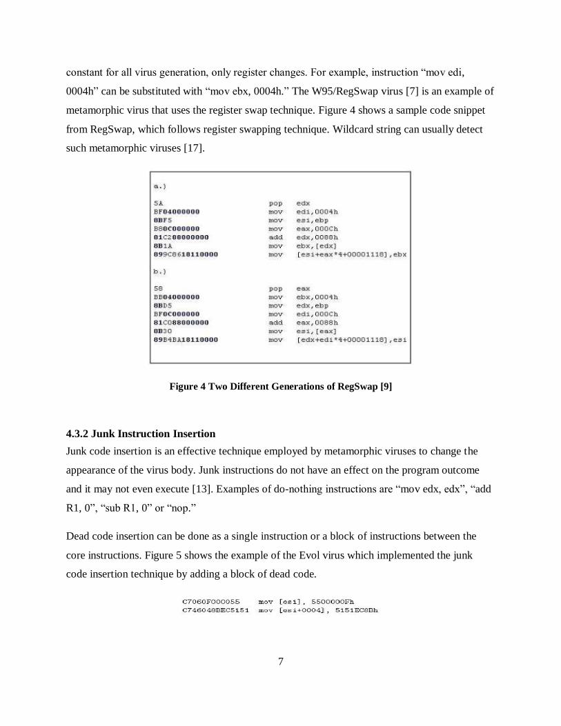

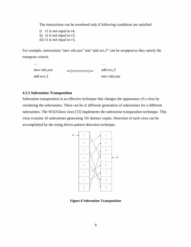
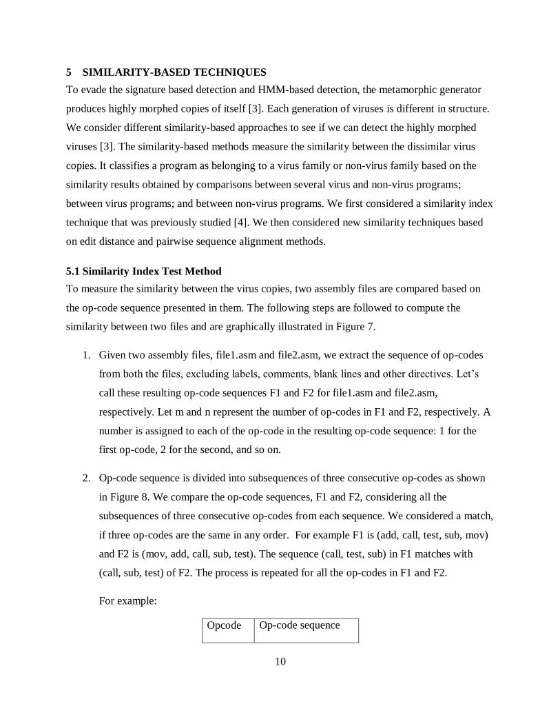
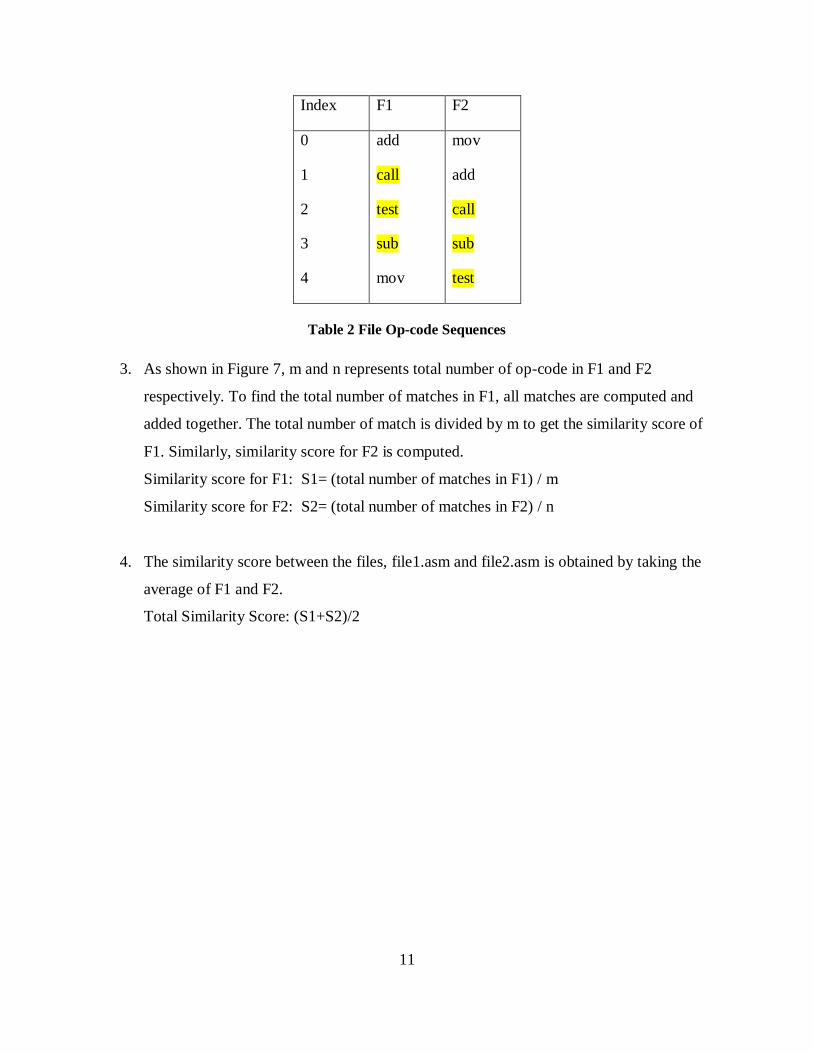
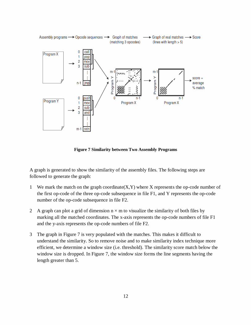

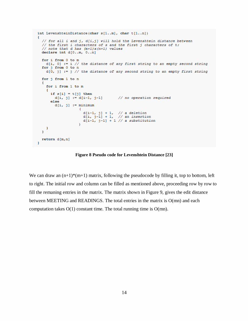
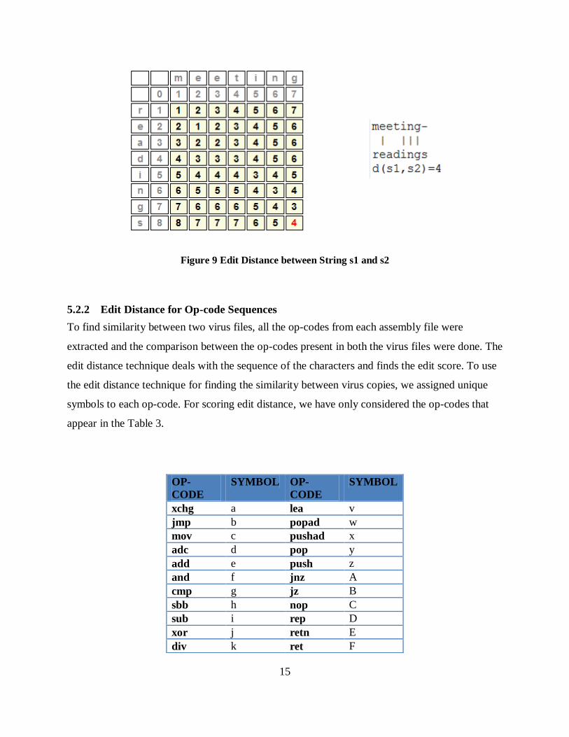


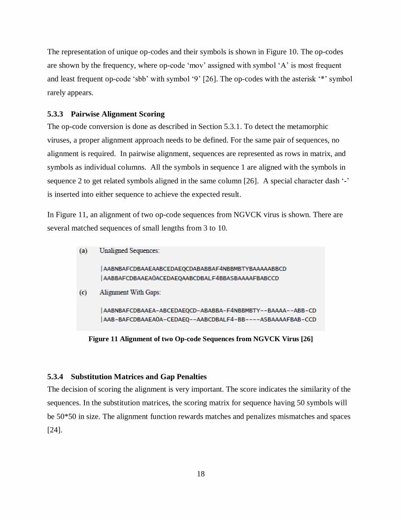


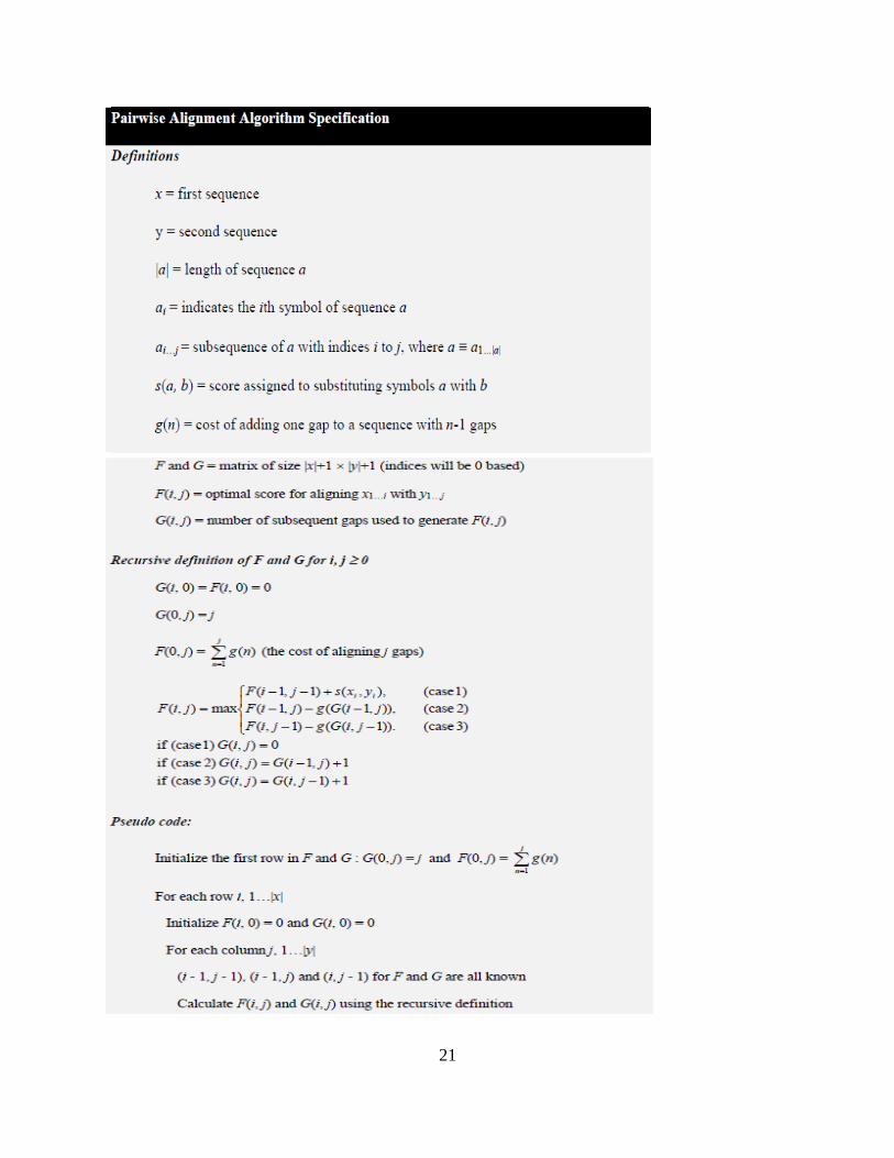
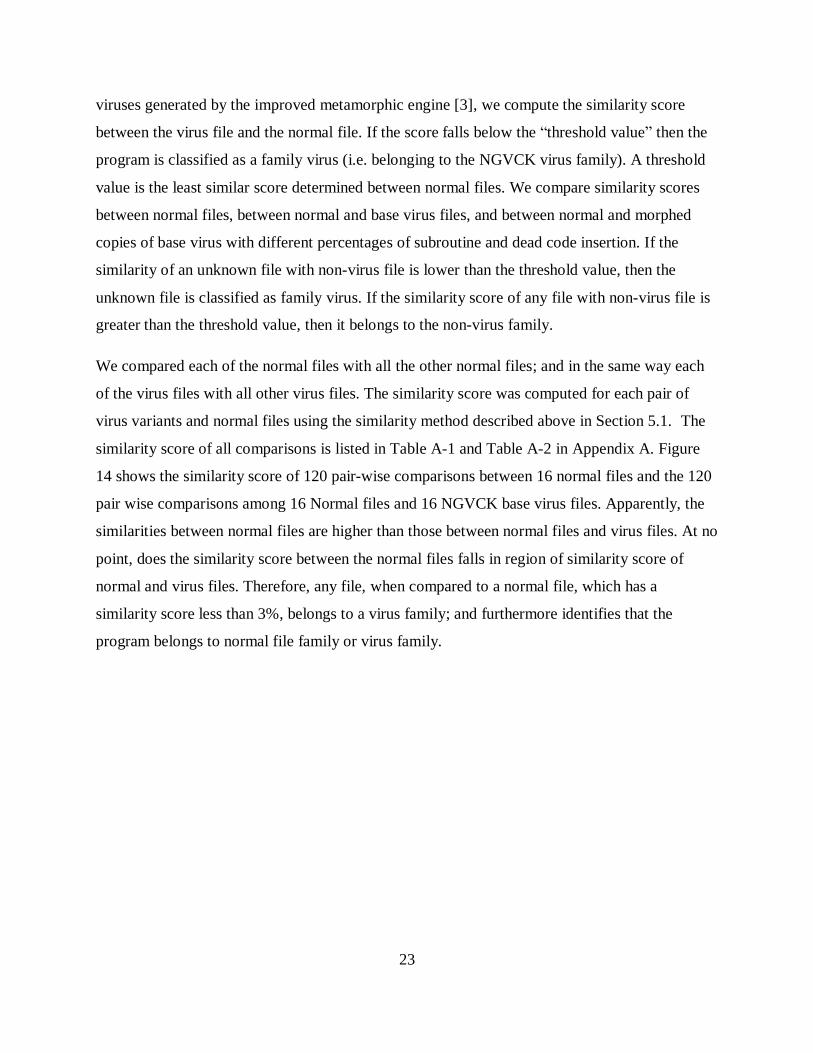


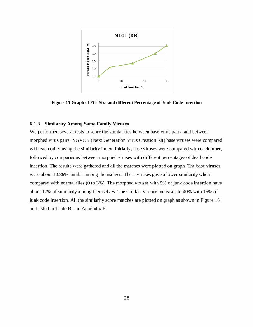


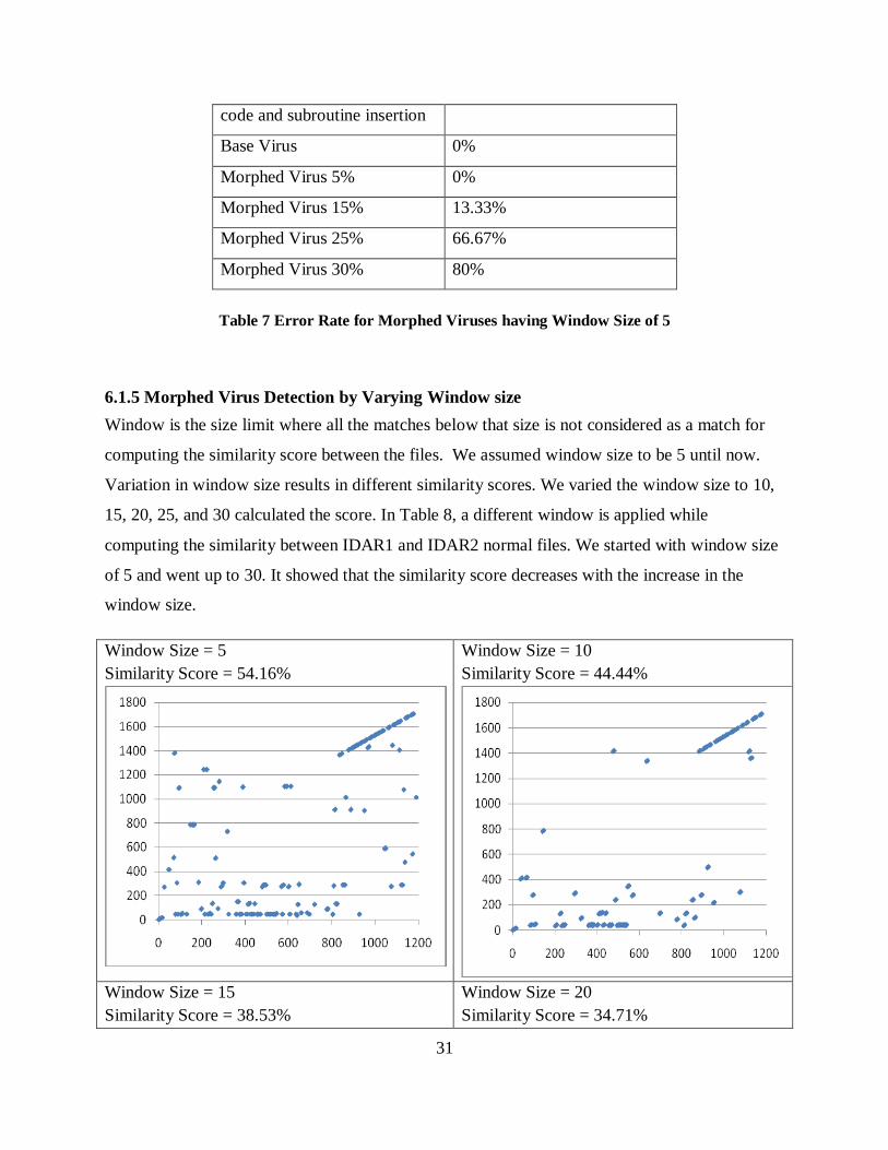


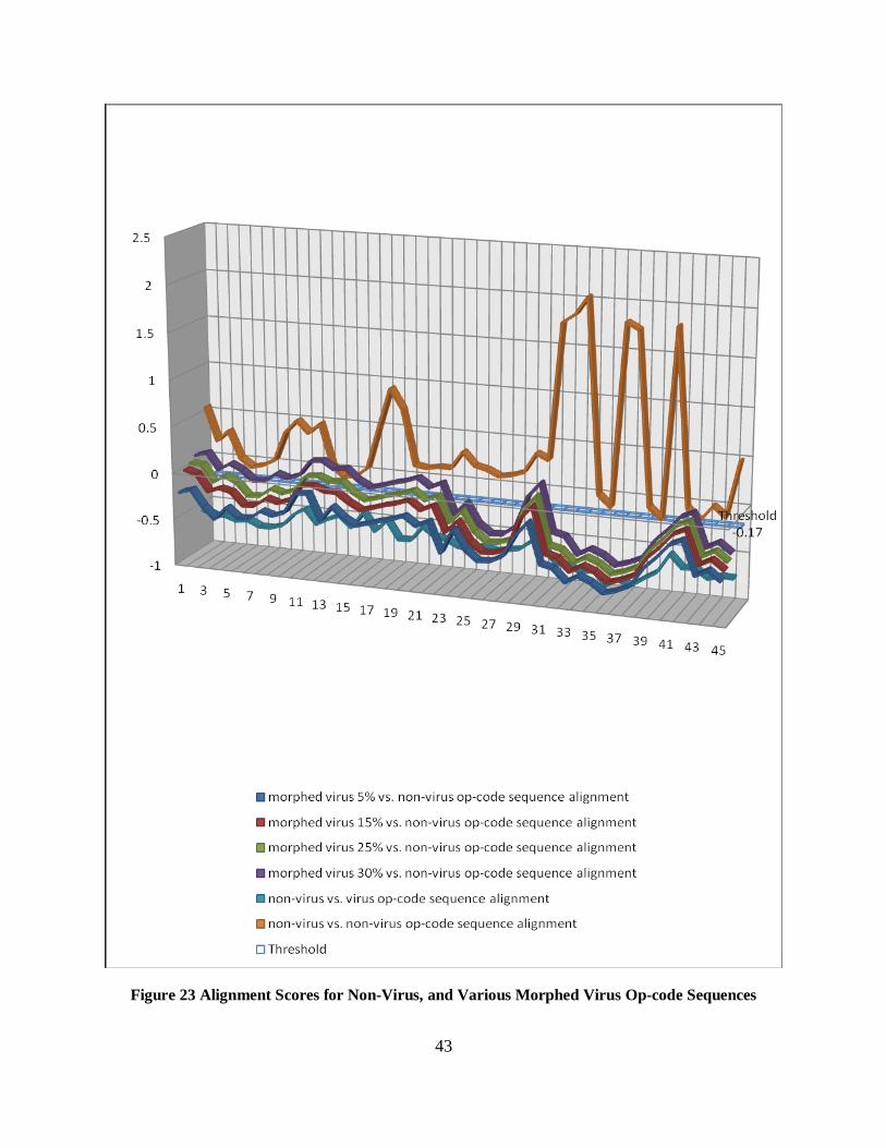


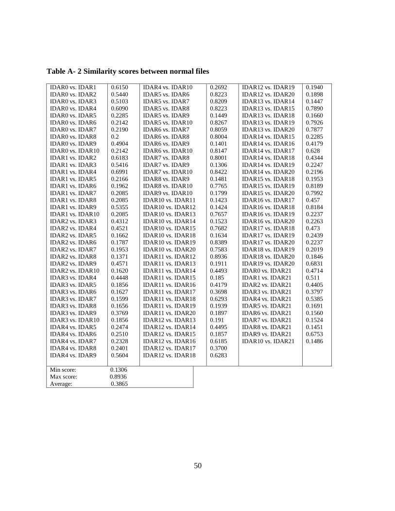


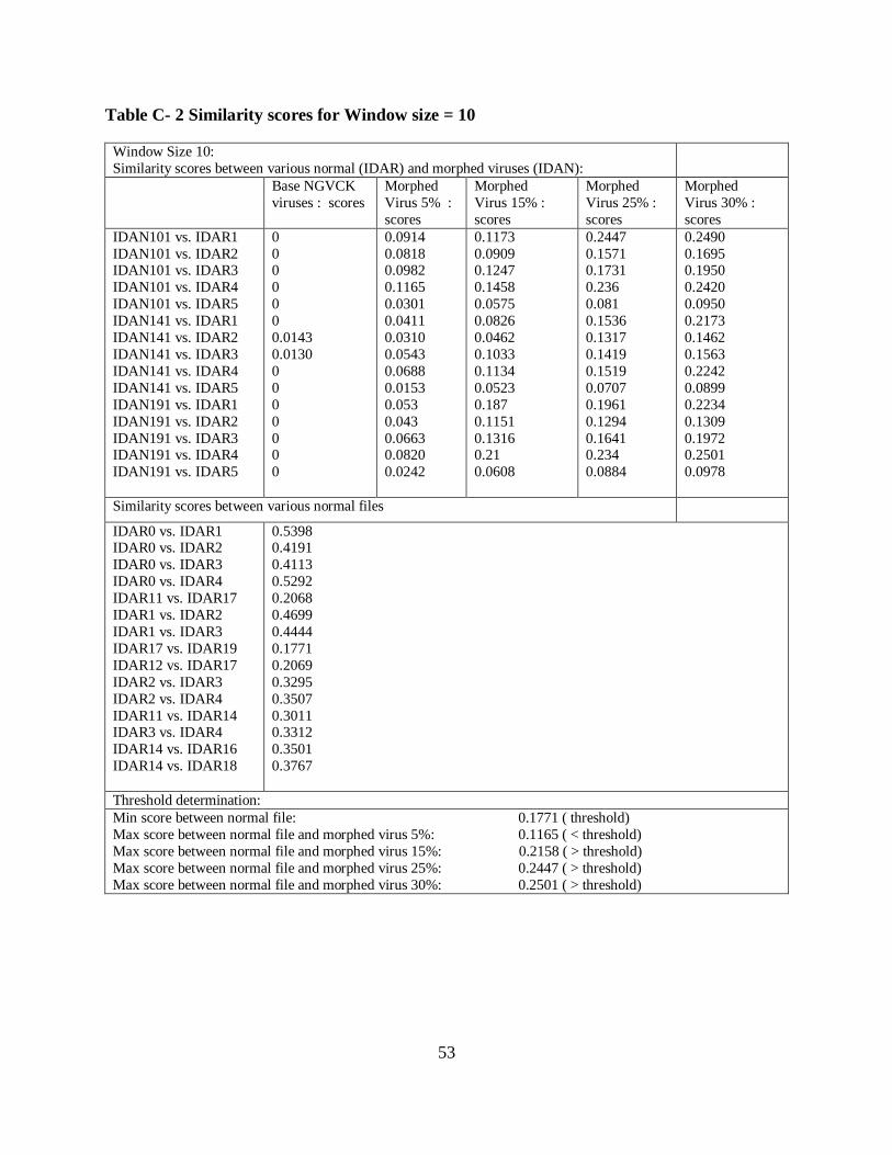


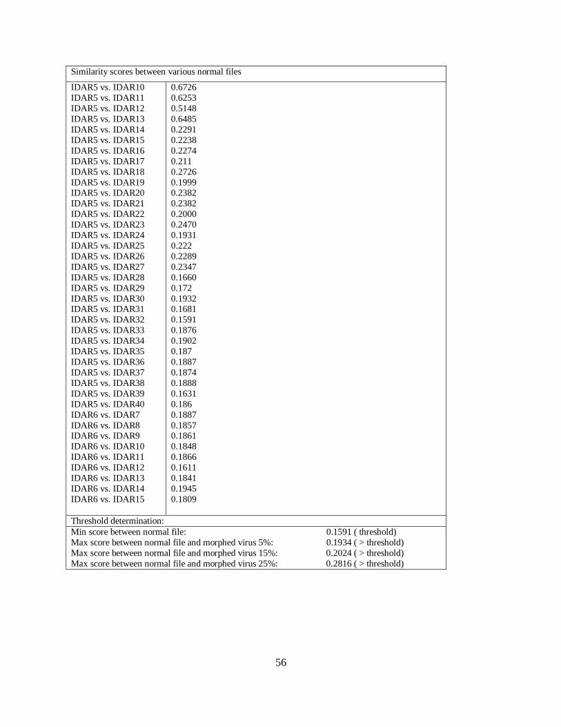


![ANALYSIS AND DETECTION OF METAMORPHIC COMPUTER … · “A computer virus is a program that recursively and explicitly copies a possibly evolved version of itself” [19]. A virus](https://static.documents.pub/doc/80x56/5f262fa66c6f7f714c643bf3/analysis-and-detection-of-metamorphic-computer-aoea-computer-virus-is-a-program.jpg)


![Hunting for metamorphic engines - Ptolemy Project...Hunting for metamorphic engines 213 Fig. 1 Shapes of a metamorphic virus [24] n! different viruses.W32/Ghost has ten subroutines,](https://static.documents.pub/doc/80x56/5f990ab0f1bb5023eb347191/hunting-for-metamorphic-engines-ptolemy-project-hunting-for-metamorphic-engines.jpg)


