TO Path Interpolation ___________________ ___________________ _________________________________________________________________________ ___________________ SIMOTION Motion Control TO Path Interpolation Function Manual 11/2010 Preface Overview of Path Interpolation 1 Basics of Path Interpolation 2 Configuring the Path Object 3 Sample Project for the Path Interpolation 4 Programming/homing path interpolation 5 Appendix A A
Transcript
�TO Path Interpolation�
___________________
___________________
___________________
___________________
___________________
___________________
___________________
SIMOTION
Motion ControlTO Path Interpolation
Function Manual
11/2010
Preface
Overview of Path Interpolation
1
Basics of Path Interpolation
2
Configuring the Path Object
3
Sample Project for the Path Interpolation
4
Programming/homing path interpolation
5
Appendix A
A
Legal information
Legal information Warning notice system
This manual contains notices you have to observe in order to ensure your personal safety, as well as to prevent damage to property. The notices referring to your personal safety are highlighted in the manual by a safety alert symbol, notices referring only to property damage have no safety alert symbol. These notices shown below are graded according to the degree of danger.
DANGER indicates that death or severe personal injury will result if proper precautions are not taken.
WARNING indicates that death or severe personal injury may result if proper precautions are not taken.
CAUTION with a safety alert symbol, indicates that minor personal injury can result if proper precautions are not taken.
CAUTION without a safety alert symbol, indicates that property damage can result if proper precautions are not taken.
NOTICE indicates that an unintended result or situation can occur if the corresponding information is not taken into account.
If more than one degree of danger is present, the warning notice representing the highest degree of danger will be used. A notice warning of injury to persons with a safety alert symbol may also include a warning relating to property damage.
Qualified Personnel The product/system described in this documentation may be operated only by personnel qualified for the specific task in accordance with the relevant documentation for the specific task, in particular its warning notices and safety instructions. Qualified personnel are those who, based on their training and experience, are capable of identifying risks and avoiding potential hazards when working with these products/systems.
Proper use of Siemens products Note the following:
WARNING Siemens products may only be used for the applications described in the catalog and in the relevant technical documentation. If products and components from other manufacturers are used, these must be recommended or approved by Siemens. Proper transport, storage, installation, assembly, commissioning, operation and maintenance are required to ensure that the products operate safely and without any problems. The permissible ambient conditions must be adhered to. The information in the relevant documentation must be observed.
Trademarks All names identified by ® are registered trademarks of the Siemens AG. The remaining trademarks in this publication may be trademarks whose use by third parties for their own purposes could violate the rights of the owner.
Disclaimer of Liability We have reviewed the contents of this publication to ensure consistency with the hardware and software described. Since variance cannot be precluded entirely, we cannot guarantee full consistency. However, the information in this publication is reviewed regularly and any necessary corrections are included in subsequent editions.
Siemens AG Industry Sector Postfach 48 48 90026 NÜRNBERG GERMANY
Content This document is part of the Description of System and Function documentation package.
Scope This manual applies to SIMOTION SCOUT in association with the SIMOTION Cam or Cam_ext technology package for product version 4.2.
Chapters in this manual The following is a list of sections included in this manual along with a description of the information presented in each section.
Chapters in this manual The following describes the purpose and objectives of the manual: ● Overview of Path Interpolation
This chapter contains an overview of the TO functionality and a definition of the terms. ● Basics of Path Interpolation
This chapter explains the basic setting options and functions of the Path Interpolation technology object.
● Configuring the Path Object This chapter explains the configuration procedure with reference to various tasks.
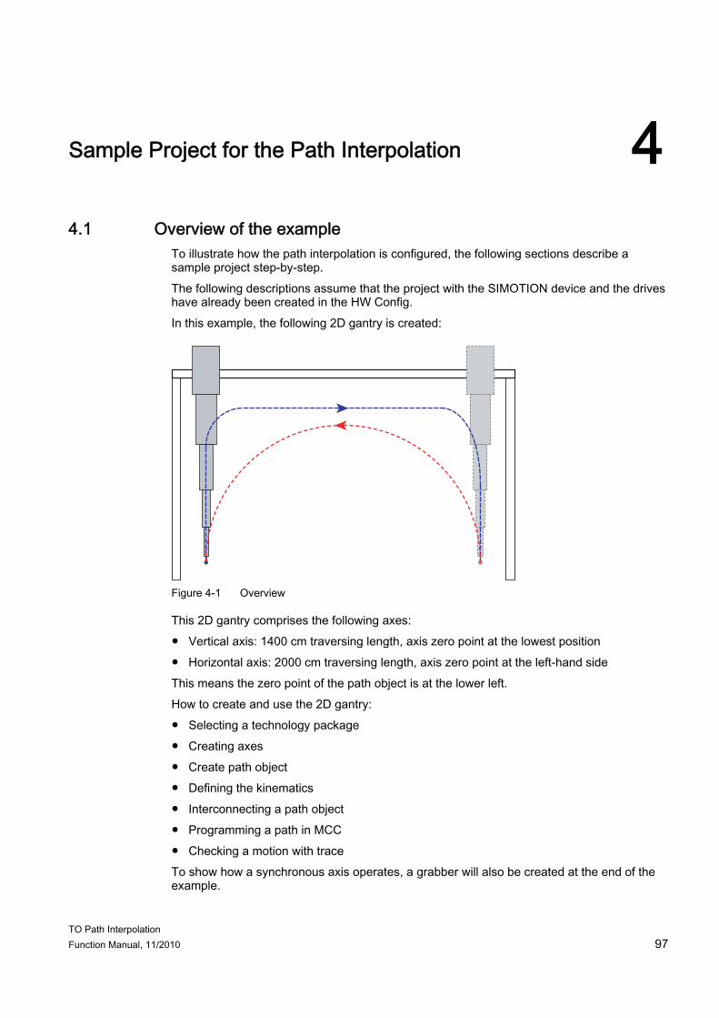
● Sample Project for the Path Interpolation In this chapter a sample project for the path interpolation is implemented.
● Programming/homing path interpolation This chapter explains the commands and functions in greater detail.
● Appendix A The specific kinematics with TrafoID 1001 are explained in this chapter.
● Index Keyword index for locating information.
SIMOTION Documentation An overview of the SIMOTION documentation can be found in a separate list of references. This documentation is included as electronic documentation in the scope of delivery of SIMOTION SCOUT. It comprises 10 documentation packages.
Preface
TO Path Interpolation 4 Function Manual, 11/2010
The following documentation packages are available for SIMOTION V4.2: ● SIMOTION Engineering System ● SIMOTION System and Function Descriptions ● SIMOTION Service and Diagnostics ● SIMOTION IT ● SIMOTION Programming ● SIMOTION Programming - References ● SIMOTION C ● SIMOTION P ● SIMOTION D ● SIMOTION Supplementary Documentation
Hotline and Internet addresses
Additional information Click the following link to find information on the the following topics:
● Ordering documentation/overview of documentation
● Additional links to download documents
● Using documentation online (find and search in manuals/information) http://www.siemens.com/motioncontrol/docu Please send any questions about the technical documentation (e.g. suggestions for improvement, corrections) to the following e-mail address: [email protected]
My Documentation Manager Click the following link for information on how to compile documentation individually on the basis of Siemens content and how to adapt this for the purpose of your own machine documentation: http://www.siemens.com/mdm
Training Click the following link for information on SITRAIN - Siemens training courses for automation products, systems and solutions: http://www.siemens.com/sitrain
Preface
TO Path Interpolation Function Manual, 11/2010 5
FAQs You can find Frequently Asked Questions on the Service&Support pages under Product Support: http://support.automation.siemens.com
Technical support Country-specific telephone numbers for technical support are provided on the Internet under Contact: http://www.siemens.com/automation/service&support
Preface
TO Path Interpolation 6 Function Manual, 11/2010
TO Path Interpolation Function Manual, 11/2010 7
Table of Contents
Preface ...................................................................................................................................................... 3 1 Overview of Path Interpolation................................................................................................................. 11
1.1 Overview of Functions .................................................................................................................11 1.2 Terminology .................................................................................................................................12
2 Basics of Path Interpolation ..................................................................................................................... 15 2.1 Path interpolation .........................................................................................................................15 2.2 Coordinate system .......................................................................................................................17 2.3 Modulo properties ........................................................................................................................17 2.4 Units .............................................................................................................................................18 2.5 Path interpolation types ...............................................................................................................18 2.5.1 Path interpolation types ...............................................................................................................18 2.5.2 Structure of commands for path interpolation..............................................................................19 2.5.3 Linear paths .................................................................................................................................21 2.5.4 Circular paths...............................................................................................................................22 2.5.4.1 Circular paths...............................................................................................................................22 2.5.4.2 Circular path in a main plane with radius, end point, and orientation..........................................22 2.5.4.3 Circle using center and angle ......................................................................................................23 2.5.4.4 Circular path using intermediate point and end point ..................................................................25 2.5.5 Polynomial paths..........................................................................................................................26 2.5.5.1 Polynomial paths..........................................................................................................................26 2.5.5.2 Polynomial path - direct specification of the polynomial coefficients ...........................................28 2.5.5.3 Polynomial paths - explicit specification of the starting point data...............................................28 2.5.5.4 Polynomial paths - attach continuously .......................................................................................30 2.6 Path dynamics..............................................................................................................................31 2.6.1 Path dynamics..............................................................................................................................31 2.6.2 Preset path dynamics ..................................................................................................................32 2.6.3 Limiting the path dynamics ..........................................................................................................32 2.7 Stopping and resuming path motion ............................................................................................35 2.8 Path behavior at motion end........................................................................................................36 2.8.1 Path behavior at motion end........................................................................................................36 2.8.2 Stopping at motion end ................................................................................................................37 2.8.3 Blending with dynamic adaptation ...............................................................................................37 2.8.4 Blending without dynamic adaptation ..........................................................................................38 2.9 Display and monitoring options on the axis .................................................................................38 2.10 Allowance for axis-specific traversing range limits ......................................................................39 2.11 Behavior of path motion when an error occurs on a participating path axis or positioning
axis...............................................................................................................................................39 2.12 Functionality of path-synchronous motion ...................................................................................40 2.12.1 Functionality of path-synchronous motion ...................................................................................40 2.12.2 Specification of path-synchronous motion ...................................................................................40 2.12.3 Dynamics of path-synchronous motion........................................................................................41
Table of Contents
TO Path Interpolation 8 Function Manual, 11/2010
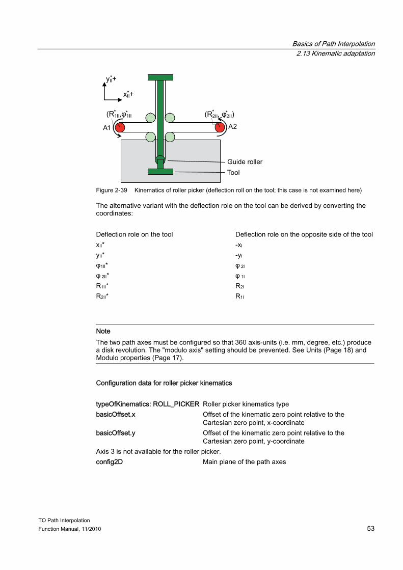
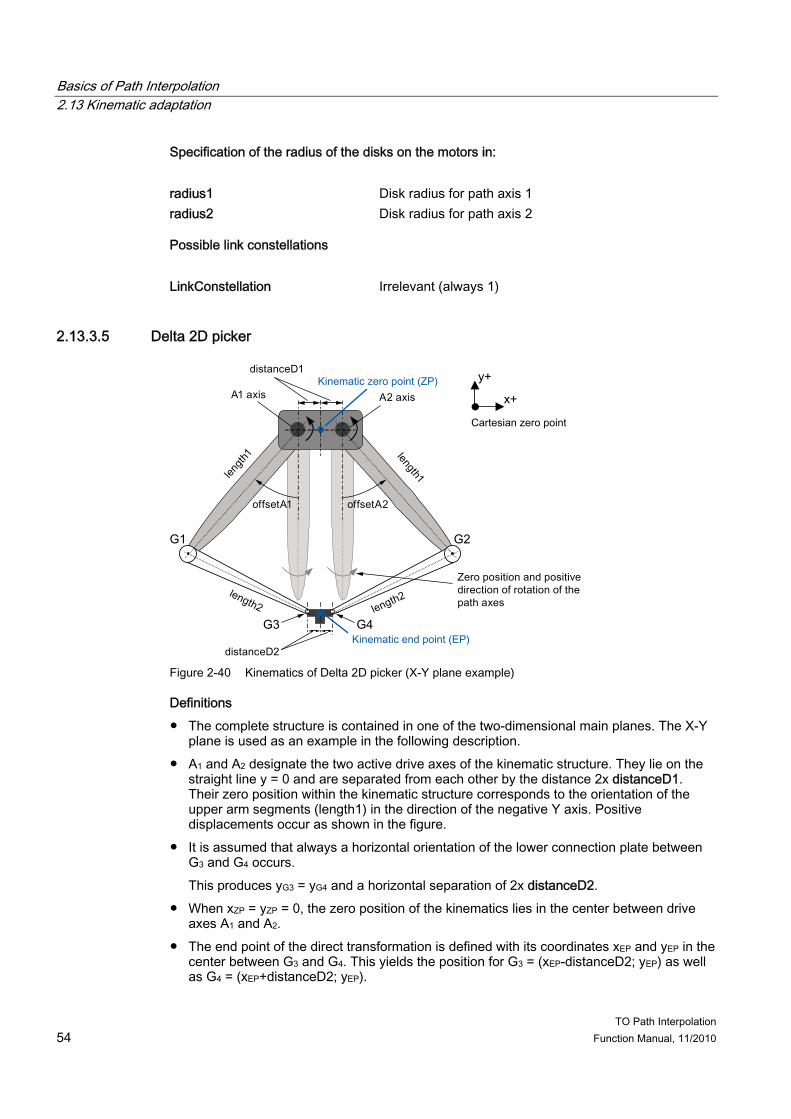
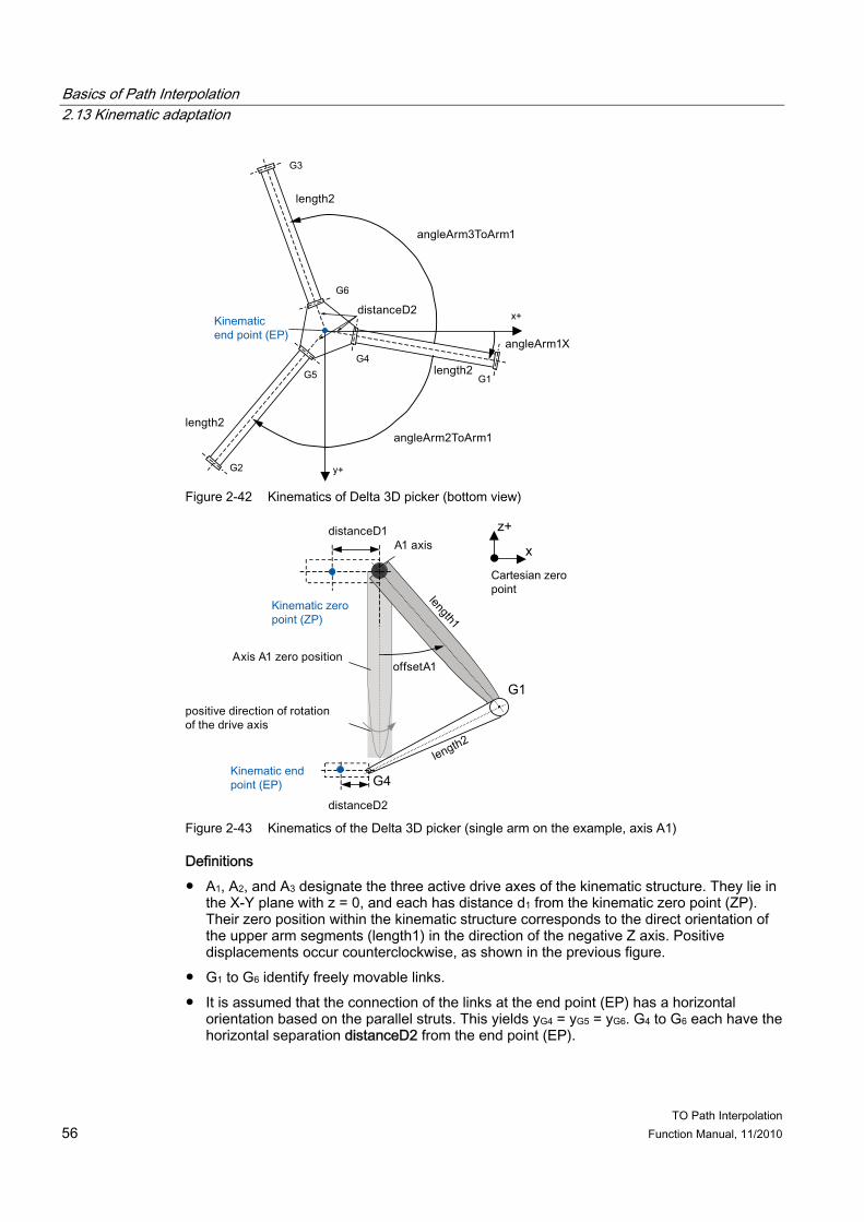
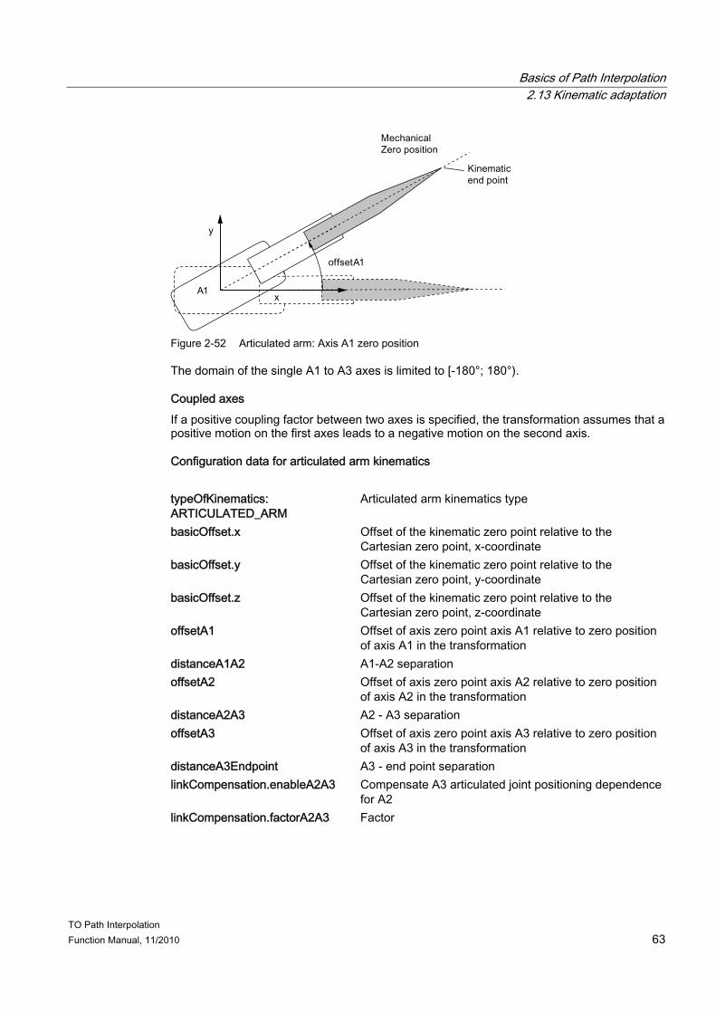
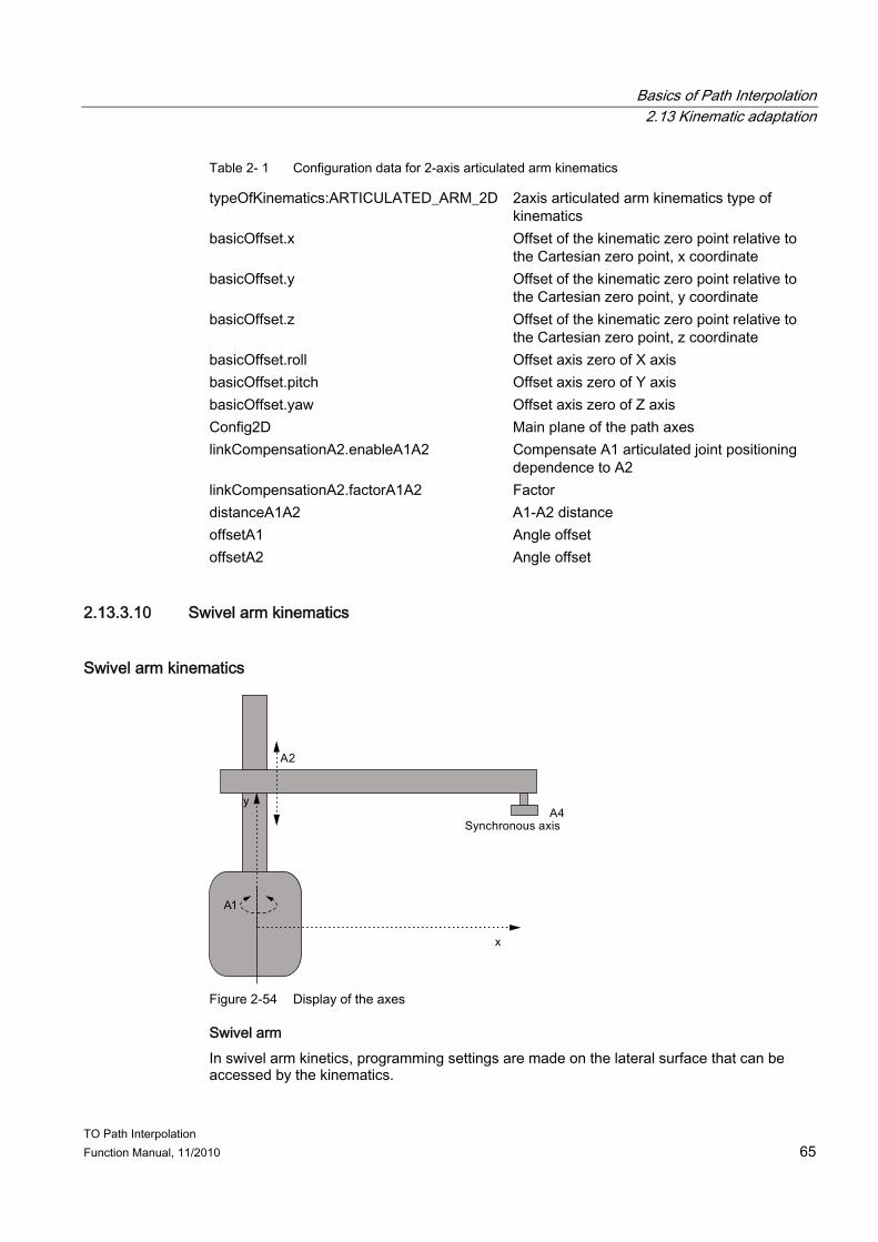
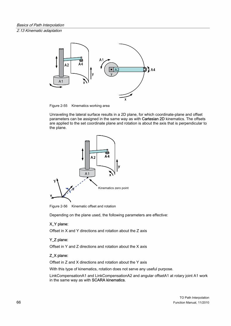
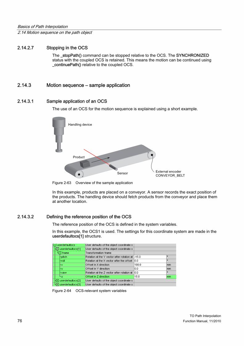
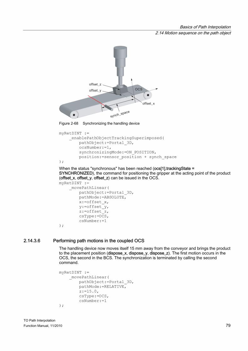
2.12.4 Path blending with a path-synchronous motion .......................................................................... 41 2.12.5 Output of the path distance to the positioning axis ..................................................................... 42 2.12.6 Output of Cartesian coordinates using the MotionOut Interface................................................. 42 2.13 Kinematic adaptation................................................................................................................... 42 2.13.1 Kinematic adaptation................................................................................................................... 42 2.13.2 Kinematic adaptation – fundamentals ......................................................................................... 42 2.13.2.1 Scope of the transformation functionality.................................................................................... 42 2.13.2.2 Reference points ......................................................................................................................... 43 2.13.2.3 System variables for path interpolation and transformation on the path object.......................... 43 2.13.2.4 Transformation of the dynamic values ........................................................................................ 45 2.13.2.5 Differentiation of link constellations............................................................................................. 45 2.13.2.6 Information commands for the kinematic transformation............................................................ 45 2.13.2.7 Axis-specific zero point offset in the transformation ................................................................... 46 2.13.2.8 Offset of the kinematic zero point relative to the Cartesian zero point ....................................... 47 2.13.3 Supported kinematics.................................................................................................................. 48 2.13.3.1 Supported kinematics and their assignment ............................................................................... 48 2.13.3.2 Configuration screens ................................................................................................................. 49 2.13.3.3 Cartesian 2D/3D gantries............................................................................................................ 51 2.13.3.4 Roller picker ................................................................................................................................ 52 2.13.3.5 Delta 2D picker............................................................................................................................ 54 2.13.3.6 Delta 3D picker............................................................................................................................ 55 2.13.3.7 SCARA kinematics...................................................................................................................... 58 2.13.3.8 Articulated arm kinematics .......................................................................................................... 61 2.13.3.9 2axis articulated arm kinematics................................................................................................. 64 2.13.3.10 Swivel arm kinematics ........................................................................................................... 65 2.13.3.11 Use of virtual axes ................................................................................................................. 67 2.13.3.12 Specific kinematics ................................................................................................................ 68 2.14 Motion sequence on the path object ........................................................................................... 69 2.14.1 Object coordinate system (OCS) on the path object .................................................................. 69 2.14.2 Motion sequence – fundamentals ............................................................................................... 70 2.14.2.1 Defining an OCS reference position ........................................................................................... 70 2.14.2.2 Assigning an OCS to a motion sequence reference value ......................................................... 71 2.14.2.3 Defining the translation of the position of the coupled OCS ....................................................... 72 2.14.2.4 Synchronizing motion on the path object to the coupled OCS ................................................... 73 2.14.2.5 Performing path motions in the coupled OCS............................................................................. 75 2.14.2.6 Terminate the coupling of the kinematic end point to a controlled OCS ('desynchronize') ........ 75 2.14.2.7 Stopping in the OCS ................................................................................................................... 76 2.14.3 Motion sequence – sample application ....................................................................................... 76 2.14.3.1 Sample application of an OCS.................................................................................................... 76 2.14.3.2 Defining the reference position of the OCS ................................................................................ 76 2.14.3.3 Determining the motion sequence reference value of the OCS ................................................. 77 2.14.3.4 Defining the position of the OCS relative to the motion sequence reference value ................... 78 2.14.3.5 Synchronizing motion on the path object to the coupled OCS ................................................... 78 2.14.3.6 Performing path motions in the coupled OCS............................................................................. 79 2.15 Interconnection, interconnection rules ........................................................................................ 80 2.16 Simulation operation ................................................................................................................... 81
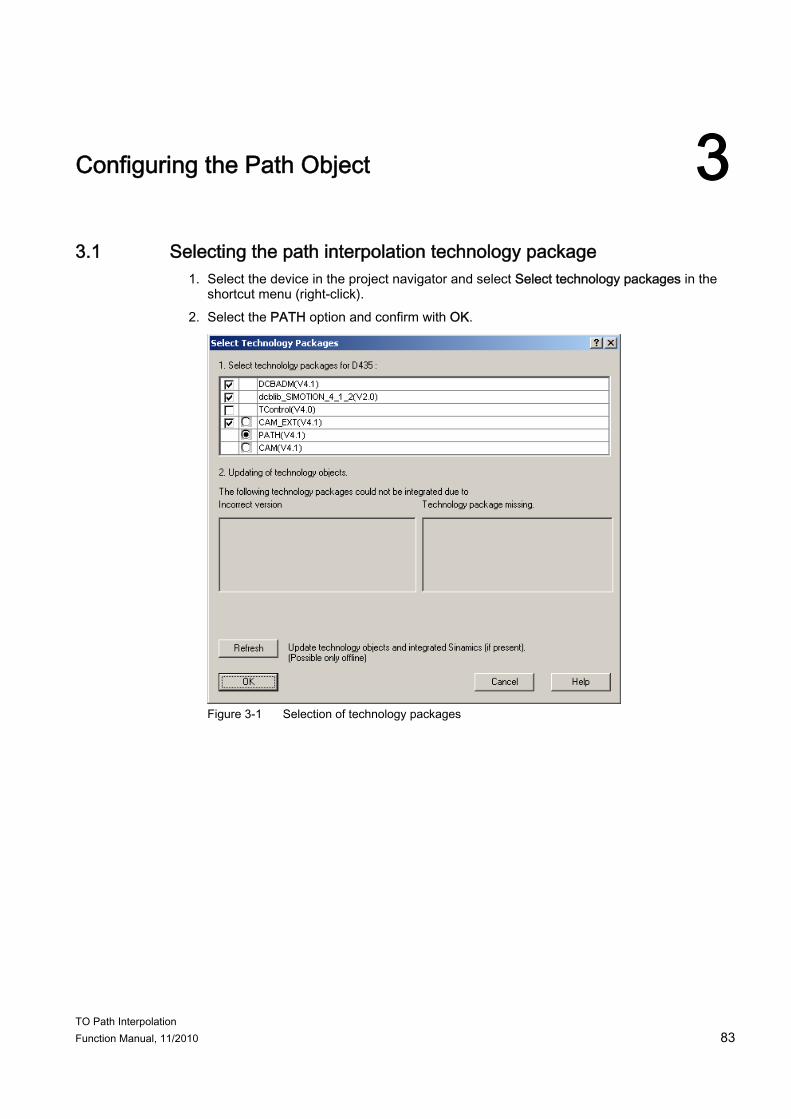
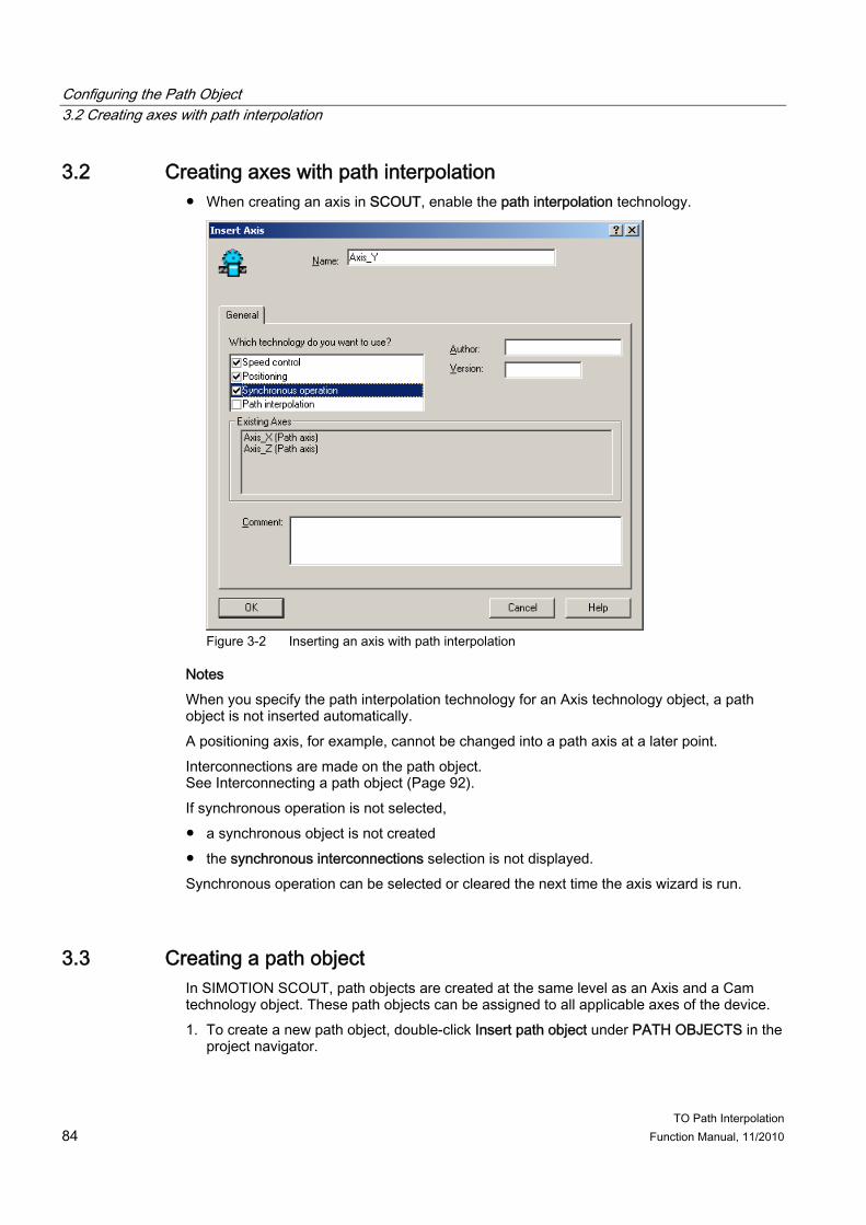
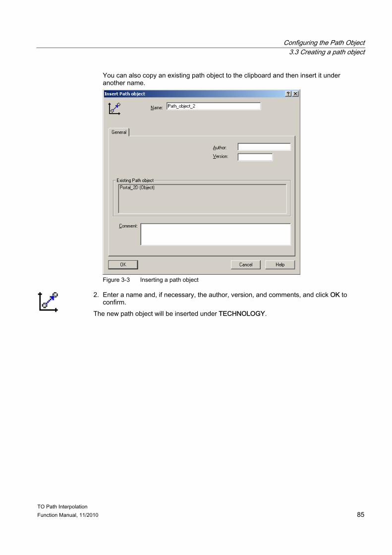
3 Configuring the Path Object..................................................................................................................... 83 3.1 Selecting the path interpolation technology package ................................................................. 83 3.2 Creating axes with path interpolation.......................................................................................... 84 3.3 Creating a path object ................................................................................................................. 84 3.4 Representation in the project navigator ...................................................................................... 86
Table of Contents
TO Path Interpolation Function Manual, 11/2010 9
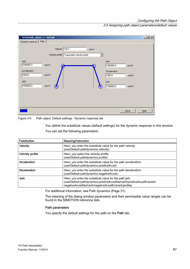
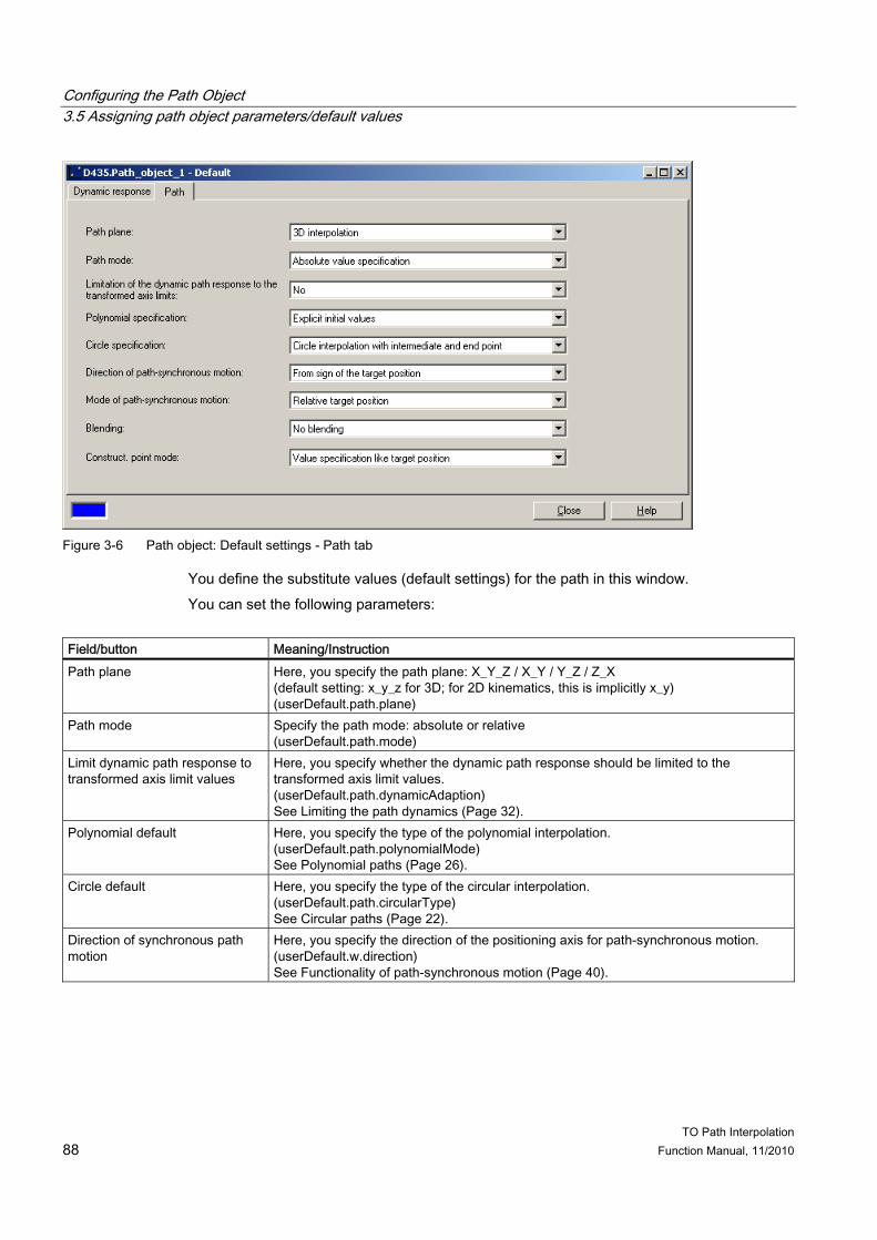
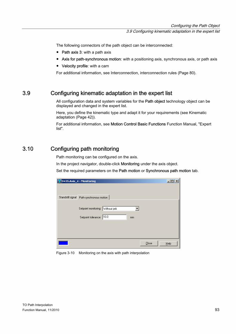
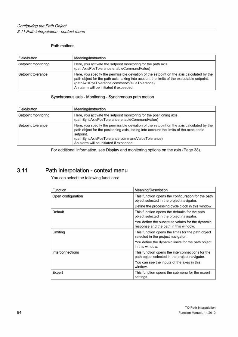
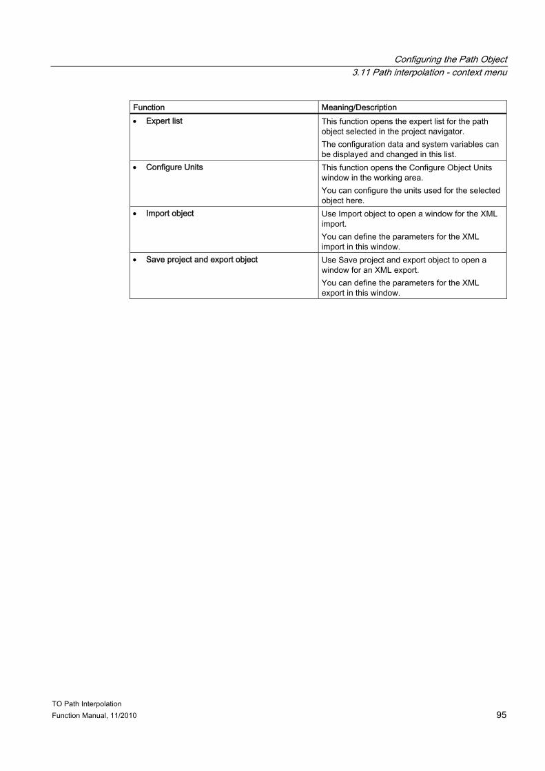
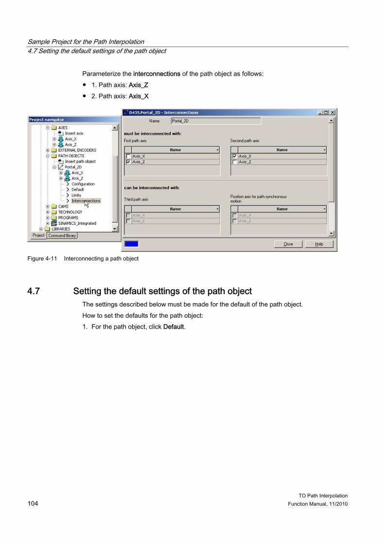
3.5 Assigning path object parameters/default values ........................................................................86 3.6 Configuring a path object .............................................................................................................90 3.7 Defining limits...............................................................................................................................91 3.8 Interconnecting a path object.......................................................................................................92 3.9 Configuring kinematic adaptation in the expert list ......................................................................93 3.10 Configuring path monitoring.........................................................................................................93 3.11 Path interpolation - context menu ................................................................................................94
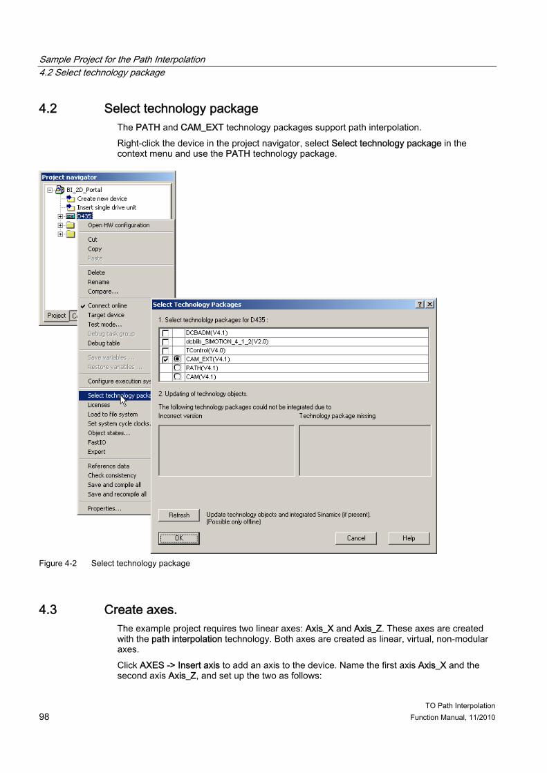
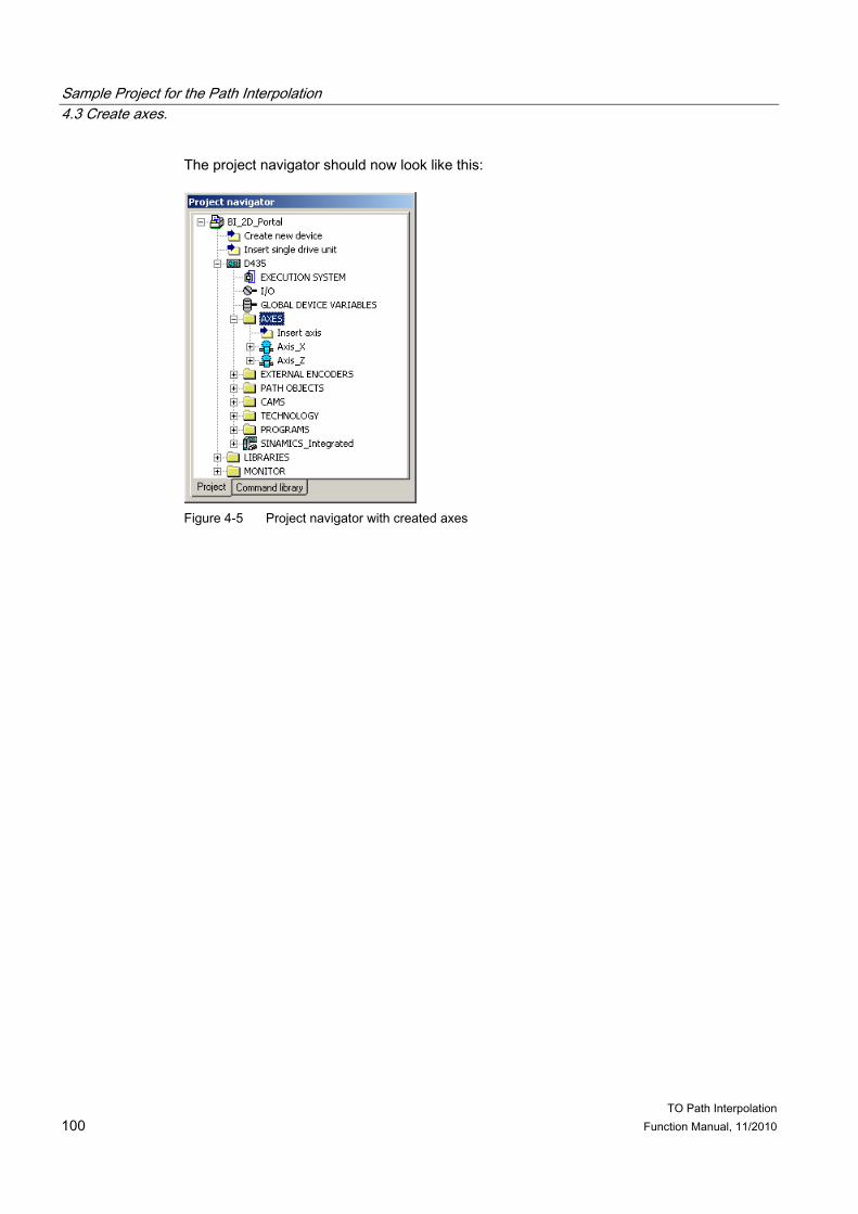
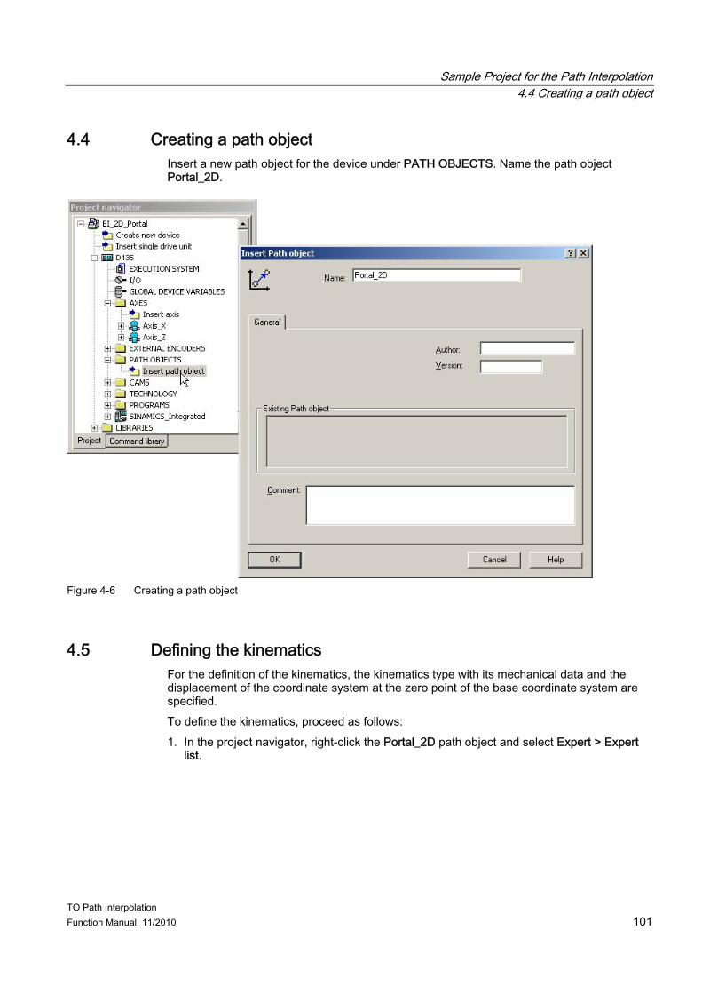
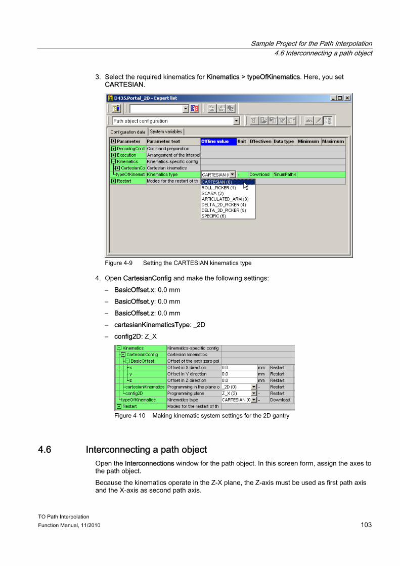
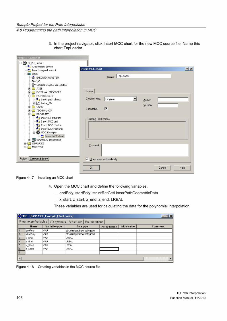
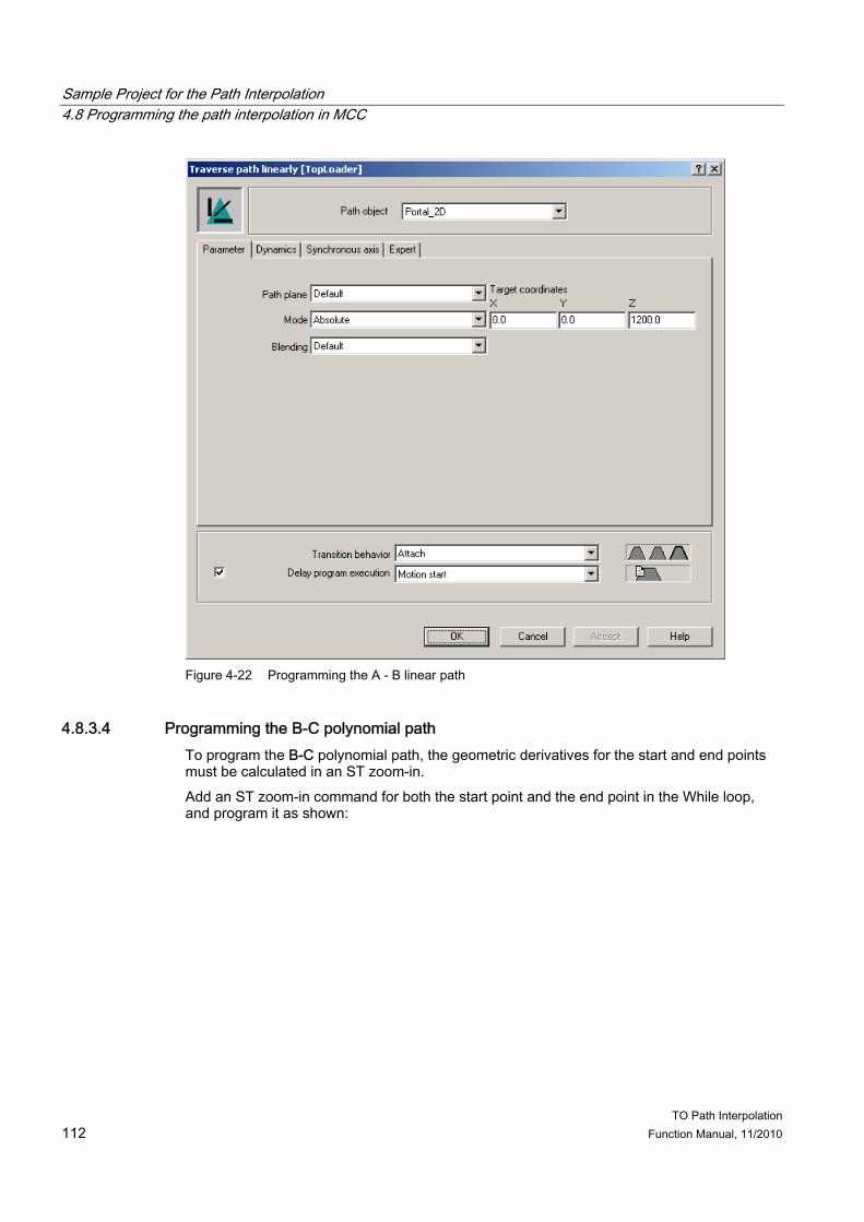
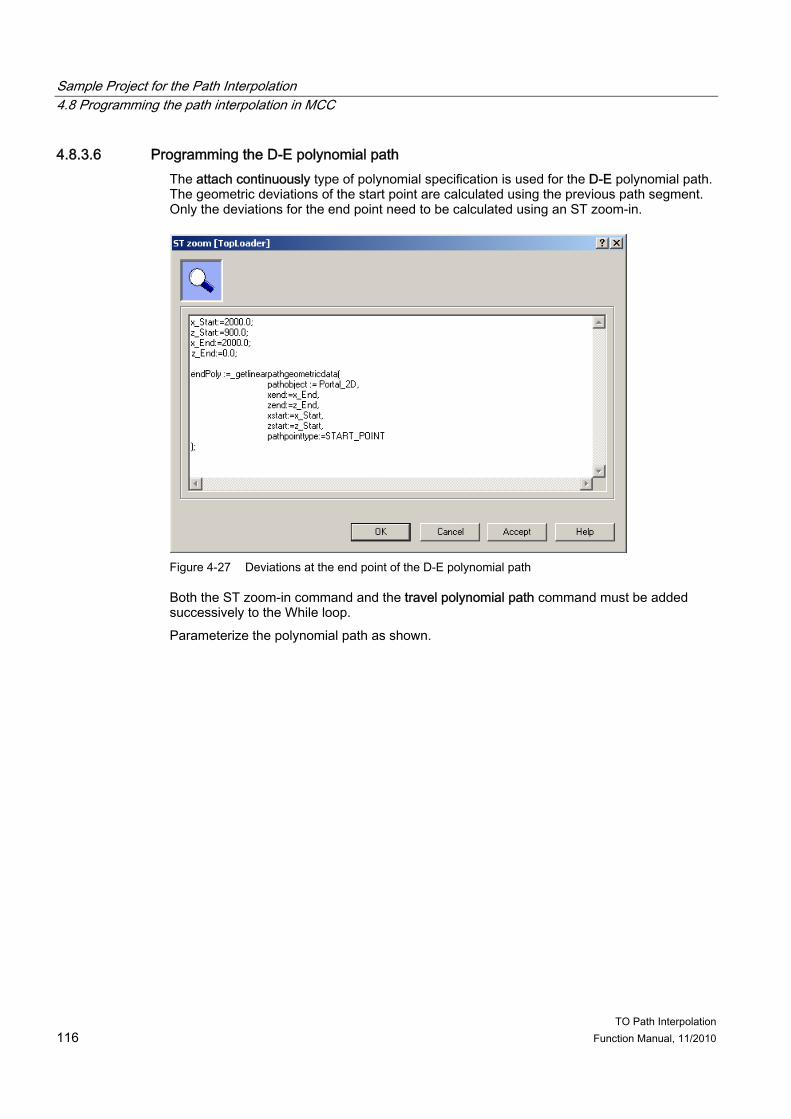
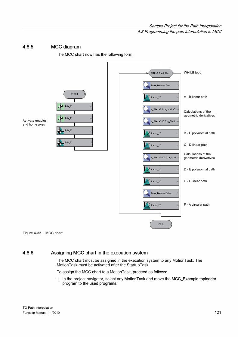
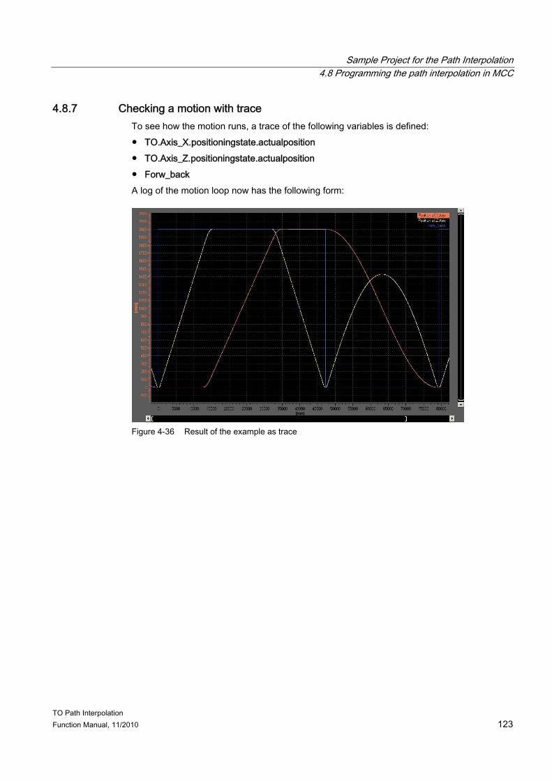
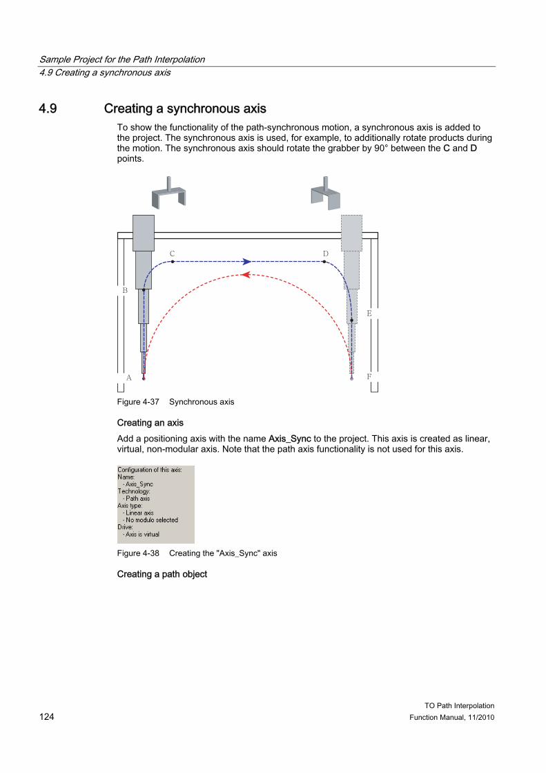
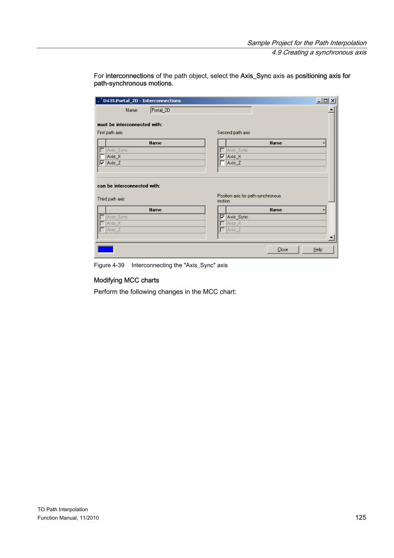
4 Sample Project for the Path Interpolation ................................................................................................ 97 4.1 Overview of the example .............................................................................................................97 4.2 Select technology package..........................................................................................................98 4.3 Create axes..................................................................................................................................98 4.4 Creating a path object................................................................................................................101 4.5 Defining the kinematics .............................................................................................................101 4.6 Interconnecting a path object.....................................................................................................103 4.7 Setting the default settings of the path object............................................................................104 4.8 Programming the path interpolation in MCC .............................................................................106 4.8.1 Programming the travel commands in MCC .............................................................................106 4.8.2 Creating the program.................................................................................................................106 4.8.3 Programming a travel loop.........................................................................................................109 4.8.3.1 Programming a travel loop.........................................................................................................109 4.8.3.2 Creating a WHILE loop ..............................................................................................................110 4.8.3.3 Programming the A - B linear path.............................................................................................110 4.8.3.4 Programming the B-C polynomial path......................................................................................112 4.8.3.5 Programming the C-D linear path ..............................................................................................115 4.8.3.6 Programming the D-E polynomial path......................................................................................116 4.8.3.7 Programming the E-F linear path...............................................................................................118 4.8.3.8 Programming the F-A return travel ............................................................................................118 4.8.4 Activating the axis enables and homing the axes......................................................................120 4.8.5 MCC diagram.............................................................................................................................121 4.8.6 Assigning MCC chart in the execution system ..........................................................................121 4.8.7 Checking a motion with trace ....................................................................................................123 4.9 Creating a synchronous axis .....................................................................................................124
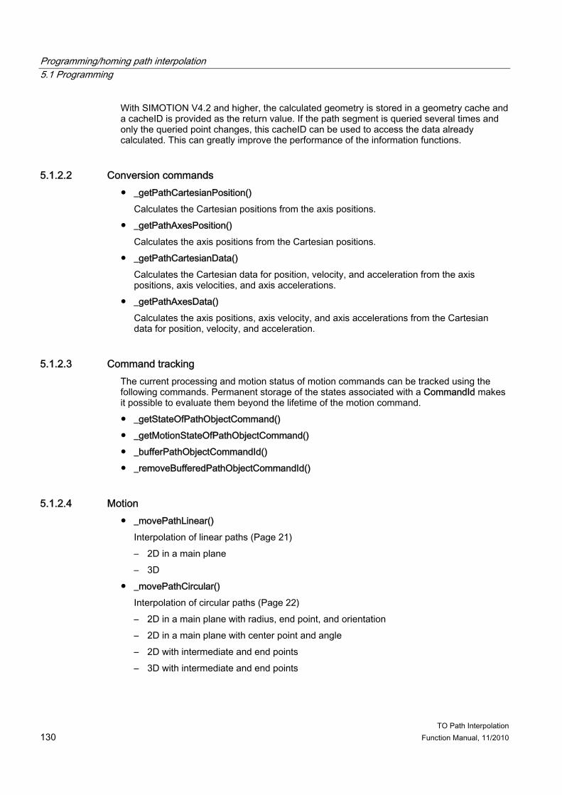
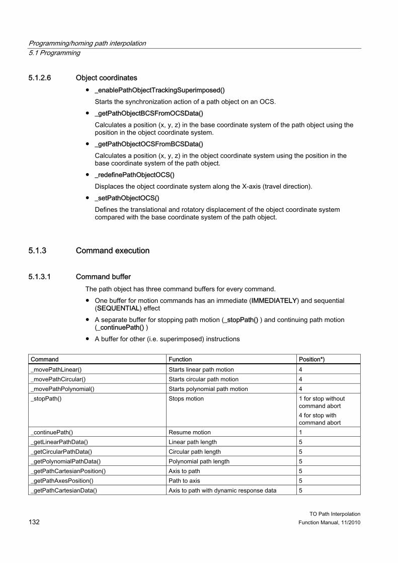
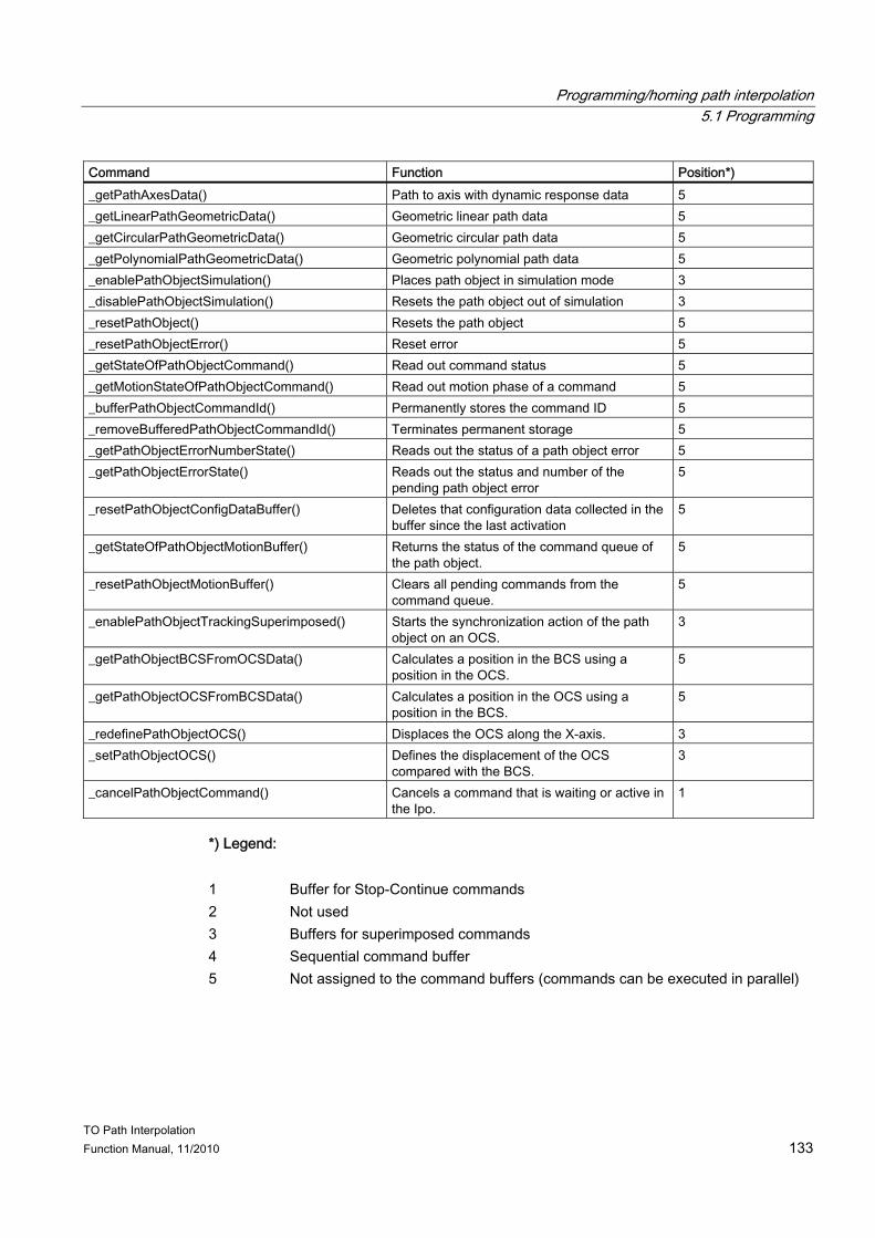
5 Programming/homing path interpolation ................................................................................................ 129 5.1 Programming..............................................................................................................................129 5.1.1 Programming: Overview ............................................................................................................129 5.1.2 Overview of commands .............................................................................................................129 5.1.2.1 Information and conversion........................................................................................................129 5.1.2.2 Conversion commands ..............................................................................................................130 5.1.2.3 Command tracking.....................................................................................................................130 5.1.2.4 Motion ........................................................................................................................................130 5.1.2.5 Object and Alarm Handling ........................................................................................................131 5.1.2.6 Object coordinates .....................................................................................................................132 5.1.3 Command execution ..................................................................................................................132 5.1.3.1 Command buffer ........................................................................................................................132 5.1.3.2 Override behavior ......................................................................................................................134 5.1.4 Interactions between the path object and the axis.....................................................................134
Table of Contents
TO Path Interpolation 10 Function Manual, 11/2010
5.1.4.1 Override behavior...................................................................................................................... 134 5.1.4.2 Sequence of effectiveness........................................................................................................ 135 5.1.4.3 Interaction with the axis............................................................................................................. 135 5.1.4.4 Interactions with other path motions ......................................................................................... 135 5.2 Local alarm response................................................................................................................ 136
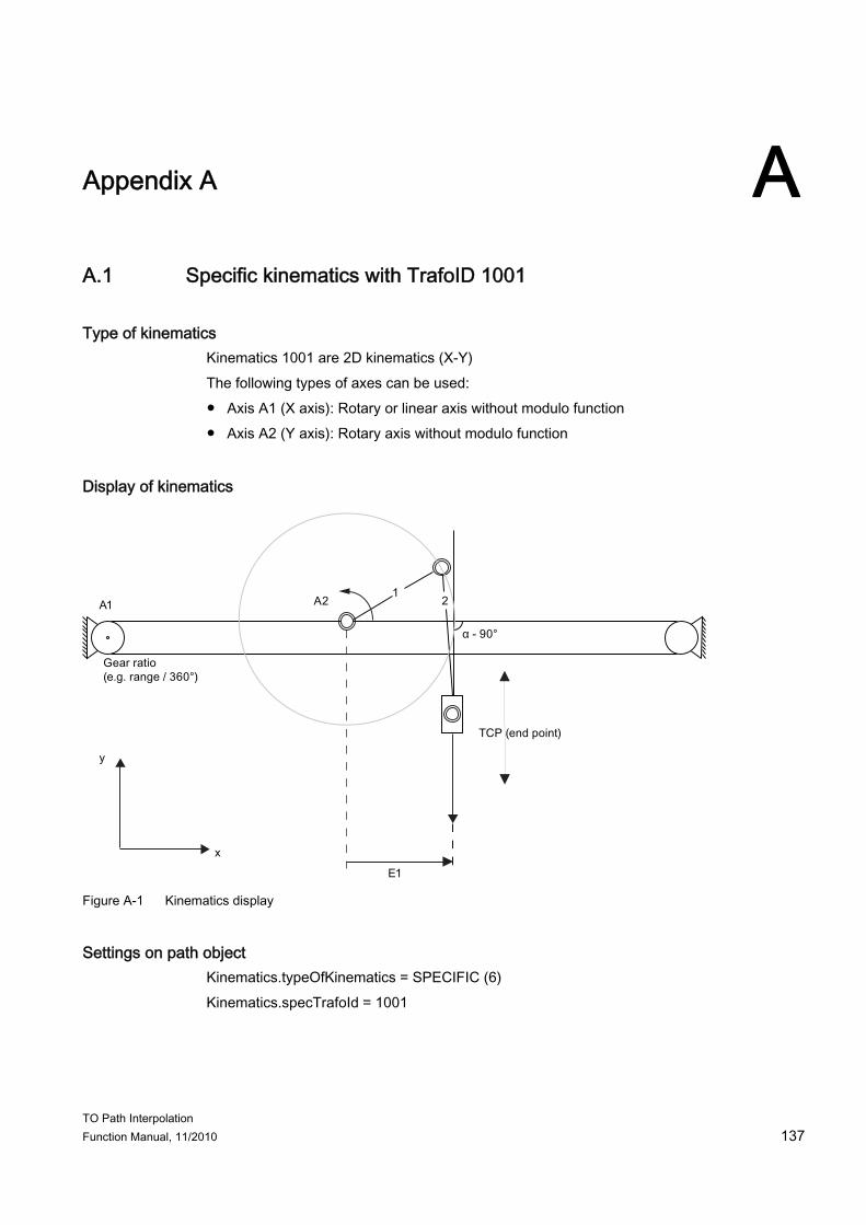
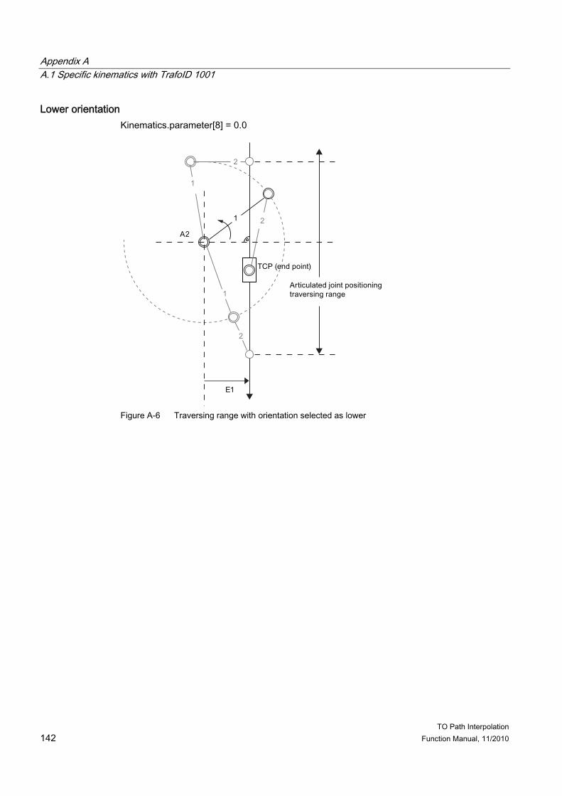
A Appendix A ............................................................................................................................................ 137 A.1 Specific kinematics with TrafoID 1001 ...................................................................................... 137
Overview of Path Interpolation 11.1 Overview of Functions
As of Version V4.1, SIMOTION provides path interpolation functionality. This functionality enables up to three path axes to travel along paths. In addition, a positioning axis can be traversed synchronously with the path. Paths can be combined from segments with linear, circular, and polynomial interpolation in 2D and 3D. The path interpolation technology is provided by the path object, which represents an independent functionality. The Path Object technology object (TO Path Object) is interconnected with path axes, and can also be interconnected with a positioning axis. The dynamic response parameters are predefined on the path motion. The path motions of individual path commands can be blended together to form a complete path with no intermediate stop. The machine kinematics are adapted to the Cartesian axes of the path coordinate system via the kinematic transformation. As of V4.1.2, the functionality is available for the synchronization of the path motions with an externally specified position value, e.g. with the motion of a conveyor. This supports the system handling for the moved conveyor. The path interpolation technology contains transformations for the following orthogonal kinematics: ● Cartesian linear aches ● SCARA ● Roller picker ● Delta 2D picker ● Delta 3D picker ● Articulated arm During a path motion, a positioning axis can be traversed synchronously with the path. The axis can approach a programmed, axis-specific target position synchronously or it can execute a motion according to the path length, thus enabling implementation of path-length-based output cams and measuring inputs. Path interpolation functions are required for such applications as feeding or withdrawal of materials to or from a machine. The application of commands for individual path segments requires a total path plan in the user program or application. DIN 66025 programming is not supported by SIMOTION.
Overview of Path Interpolation 1.2 Terminology
TO Path Interpolation 12 Function Manual, 11/2010
1.2 Terminology
Axis coordinates Coordinates of the path axes or the positioning axis with path-synchronous motion
Path interpolation Motion along a path with an assignable dynamic response. Path interpolation generates the traversing profile for the path, calculates the path interpolation points in the interpolation cycle, and uses the kinematic transformation to derive the axis setpoints for the interpolation cycle points.
Continuous-path control Motion along a path at a definable velocity. This can include a velocity-based smoothing of the segment transitions by insertion of rounded transition segments. The path interpolation function of SIMOTION Version 4.1 only covers the continuous-path control functionality to a limited extent. Therefore, this term is not used.
Path object The path object provides the functionality for the path interpolation and for other tasks connected with the path interpolation. It also contains the kinematics transformations implemented in the system.
Path axis Axis that can execute a path motion along with other path axes via a path object.
Path-axis interface Interfaces for bidirectional data exchange between the path object and interconnected path axes.
Path motion Motion resulting from the interpolation of a path motion command; output on path axes
Path interpolation grouping Several path and positioning axes connected by a path object or interpolation
Basic coordinate system (BCS) Coordinate system of path interpolation. A right-handed, rectangular coordinate system in accordance with DIN 66217 is used.
Motion sequence Permits the coupling of the kinematic end point with a coupled OCS and so, for example, the coupling with the actual value of a conveyor. This means, for example, a product can be taken from a running conveyor or placed there. As of SIMOTION V4.1.2, position details in the motion commands can be related optionally to the basic coordinate system or to an object coordinate system (OCS).
Overview of Path Interpolation 1.2 Terminology
TO Path Interpolation Function Manual, 11/2010 13
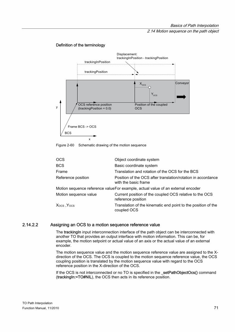
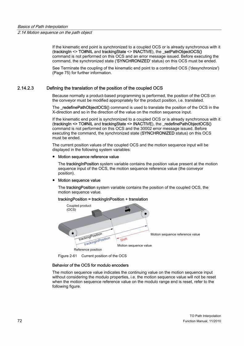
Motion sequence reference value (trackingInPosition) The value made available to the TrackingIn interface of the path object by another technology object. This can be, for example, the actual value of an external encoder.
Motion sequence value (trackingPosition) The current position of a coupled OCS with reference to the OCS reference position.
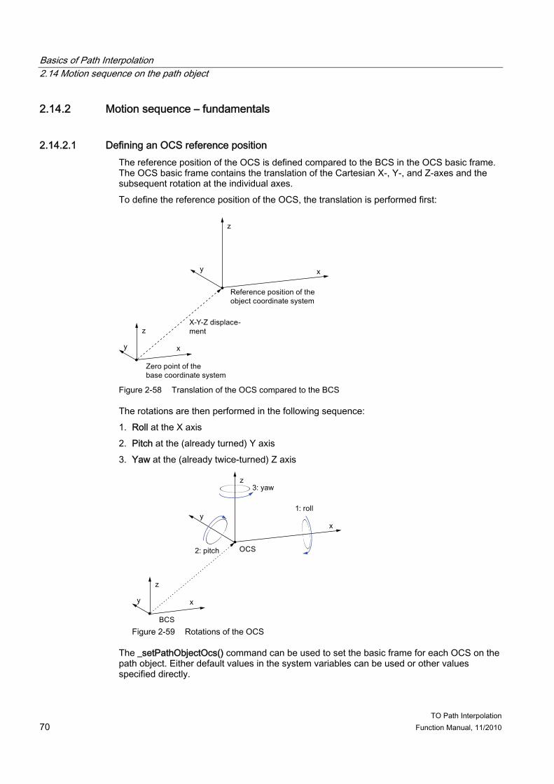
Frame transformation A frame transformation describes the position of a coordinate system relative to another coordinate system that defines, for example, the OCS reference position relative to the basic coordinate system of the path object. The frame transformation consists of translations along the X-, Y-, and Z-axes and rotations at the individual axes. For the transformation, the displacements are performed first and then the rotations in the following order: ● Roll at the X axis ● Pitch at the (already turned) Y axis ● Yaw at the (already twice-turned) Z axis
Main plane x-y, y-z, or z-x plane or a parallel plane. The third coordinate is not evaluated.
Interface for path-synchronous motion Interface for bidirectional data exchange between the path object and an interconnected positioning axis for path-synchronous motion.
Cartesian axes Axes X, Y, and Z of the path object
Kinematics The term "kinematics" in the context of robots and handling devices in motion control systems refers to the abstraction of a mechanical system onto the variables relevant for motion and motion control, i.e. the motion-capable elements (articulations) and their geometric positions relative to each other (arms).
Kinematic transformation, kinematic adaptation Conversion of specifications in Cartesian coordinates to specifications for individual path axes, and vice versa.
Circular path Path in 2D or 3D that describes a circle or an arc path.
Linear path Path in 2D or 3D that describes a straight path.
Coupled OCS An object coordinate system (OCS) coupled synchronously to the trackingIn interface.
Overview of Path Interpolation 1.2 Terminology
TO Path Interpolation 14 Function Manual, 11/2010
Object coordinate system (OCS) As of SIMOTION V4.1.2, in addition to the base coordinate system (BCS), object coordinate systems (OCS) with the path object are also available. Path motions can be specified either in the BCS or in the OCS. The object coordinate systems are defined in their reference position using frame transformations for the BCS. They can be coupled with a specified motion value in the x direction of the OCS on the TrackingIn interface.
OCS reference position Position of the OCS for the motion sequence value equal to zero. The OCS reference position for the BCS is defined using a frame transformation.
Polynomial path Path in 2D or 3D that describes a polynomial segment.
Synchronous motion, path-synchronous motion Synchronous coupling of an axis with a path motion; output on a positioning axis
TrackingIn interface The trackingIn input interconnection interface of the path object can be interconnected with another TO that provides an output interface with motion information. This can be, for example, the motion setpoint or actual value of an axis or the actual value of an external encoder.
TO Path Interpolation Function Manual, 11/2010 15
Basics of Path Interpolation 22.1 Path interpolation
The path interpolation technology provides functionality for interpolating linear, circular, and polynomial paths in two dimensions (2D) and three dimensions (3D).
Figure 2-1 Role and basic principle of the path interpolator
Objects involved in path interpolation
Figure 2-2 Objects involved in path interpolation
The path interpolation technology is made available in the Path Object technology object (TO Path Object).
Basics of Path Interpolation 2.1 Path interpolation
TO Path Interpolation 16 Function Manual, 11/2010
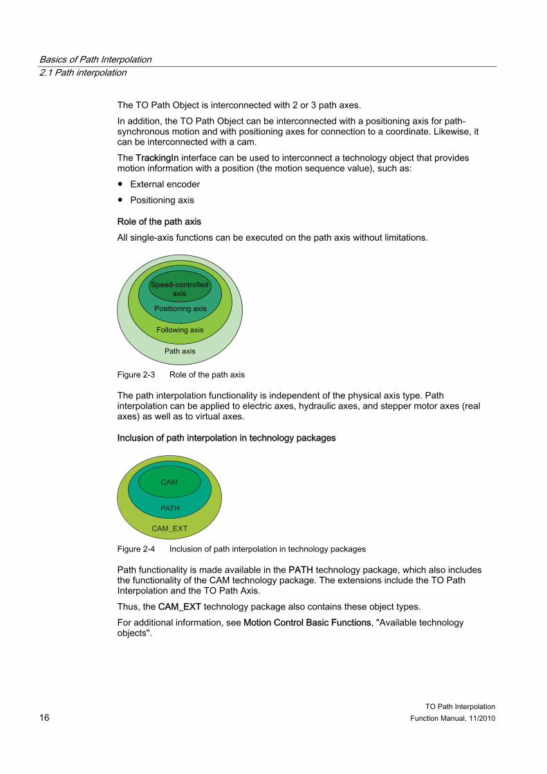
The TO Path Object is interconnected with 2 or 3 path axes. In addition, the TO Path Object can be interconnected with a positioning axis for path-synchronous motion and with positioning axes for connection to a coordinate. Likewise, it can be interconnected with a cam. The TrackingIn interface can be used to interconnect a technology object that provides motion information with a position (the motion sequence value), such as: ● External encoder ● Positioning axis
Role of the path axis All single-axis functions can be executed on the path axis without limitations.
Figure 2-3 Role of the path axis
The path interpolation functionality is independent of the physical axis type. Path interpolation can be applied to electric axes, hydraulic axes, and stepper motor axes (real axes) as well as to virtual axes.
Inclusion of path interpolation in technology packages
Figure 2-4 Inclusion of path interpolation in technology packages
Path functionality is made available in the PATH technology package, which also includes the functionality of the CAM technology package. The extensions include the TO Path Interpolation and the TO Path Axis. Thus, the CAM_EXT technology package also contains these object types. For additional information, see Motion Control Basic Functions, "Available technology objects".
Basics of Path Interpolation 2.2 Coordinate system
TO Path Interpolation Function Manual, 11/2010 17
2.2 Coordinate system The path interpolation functions require a Cartesian coordinate system. A clockwise, rectangular coordinate system in accordance with DIN 66217 is used. The user programs in this right-handed system, irrespective of the real kinematics.
z
y
x Figure 2-5 Cartesian coordinate system, right-handed system
Main planes It is easy to program two-dimensional motions (2D) directly in one of the three main planes X-Y, Y-Z, or Z-X. In this case, the third coordinate remains constant and does not have to be programmed.
Figure 2-6 Main planes in 3D
2.3 Modulo properties Both path axes and positioning axes can be used as modulo axes. However, no modulo range change for the path axis may occur in the path traversal area. The kinematic transformation does not take account of any modulo range change. Consequently, only one modulo range of the path axis can be used for the traversal area on the path object. The activation of the path interpolation defines the modulo range for the path motion.
Basics of Path Interpolation 2.4 Units
TO Path Interpolation 18 Function Manual, 11/2010
This means that the modulo transition of the axis must not be in the traversing range of the path motions. The modulo range and the modulo starting point as well as the position of the modulo range relative to the intended path travel range must be set appropriately, for example, using the settings for reference point and reference point offset during homing.
2.4 Units All axis-related values are displayed in the quantity and unit of the assigned (interconnected) axes. The Cartesian coordinates are indicated in a unit of length. The default setting for Cartesian values is [mm]. The default unit for rotary values, such as rotary angle, is [°] and calculated as degrees. The transformation calculates directly with the numerical values. There is no unit conversion for transformations provided by the system. Thus, the same units must be used for the same base value, e.g, length specification.
Note Use the same units for all objects associated with the path object that have the same reference quantities (e.g. linear axes in mm, rotary axes in °). Avoid, for example, the mixing of metric and non-metric units for the involved axes.
2.5 Path interpolation types
2.5.1 Path interpolation types
Figure 2-7 Examples of linear path in 3D, circular path in 3D, polynomial path in 3D
Basics of Path Interpolation 2.5 Path interpolation types
TO Path Interpolation Function Manual, 11/2010 19
The following interpolation modes are available for the path object: ● Linear paths (Page 21)
– 2D in a main plane – 3D
● Circular paths (Page 22) – 2D in a main plane with radius, end point, and orientation – 2D in a main plane with center point and angle – 2D with intermediate and end points – 3D with intermediate and end points
● Polynomial paths (Page 26) – 2D in a main plane with explicit specification of geometric derivatives in the start point
or with a geometrically continuous attachment – 3D with explicit specification of geometric derivatives in the start point or with a
geometrically continuous attachment – 2D with explicit specification of polynomial parameters – 3D with explicit specification of polynomial parameters
The main plane (2D) or the 3D mode in which the path motion occurs can be specified with the pathPlane parameter of the interpolation command. The third path coordinate perpendicular to the main plane is not changed in a 2D path.
2.5.2 Structure of commands for path interpolation The following path interpolation commands are available: ● Linear interpolation: _movePathLinear() ● Circular interpolation: _movePathCircular() ● Polynomial interpolation: _movePathPolynomial() These commands contain the following parameters: ● Specification of the object instance in pathObjectType ● Specification of the path plane in pathPlane
This parameter is used to set the path plane. The main plane (2D) or the 3D mode in which the path motion should occur can be specified.
● Specification of the path mode in pathMode This parameter is used to set whether the value for the end point is specified as an absolute value or whether it is to be evaluated relative to the start point.
● Specification of the end point in x, y, z ● Specification of the blending mode in blendingMode ● Specification of the merge behavior in mergeMode
Basics of Path Interpolation 2.5 Path interpolation types
TO Path Interpolation 20 Function Manual, 11/2010
● Specification of the command transition in nextCommand ● Specification of the command ID in commandId
Specifications for the linear path only ( _movePathLinear() ): (see Linear paths (Page 21) ) ● None
Specifications for the circular path only (_movePathCircular() ) (see Circular paths (Page 22) ) ● Specification of the circle type in circularType ● Specification of the circle direction in circleDirection ● Specification of the intermediate point mode in ijkMode ● Specification of the intermediate point mode in i, j, k ● Specification of the arc angle in arc ● Specification of the circle radius in radius
Specifications for the polynomial path only (_movePathPolynomial() ) (see Polynomial paths (Page 26) ) ● Specification of polynomial mode in polynomialMode ● Specification of the vector components in vector1x to vector4z
Specifications for the dynamics (see Path dynamics (Page 31) ) ● Velocity profile in velocityprofile ● Velocity in velocity ● Acceleration in positiveAccel ● Deceleration in negativeAccel ● Jerk on start of acceleration in positiveAccelStartJerk ● Jerk at acceleration end in positiveAccelEndJerk ● Jerk on start of deceleration in negativeAccelStartJerk ● Jerk at deceleration end in negativeAccelEndJerk ● Selection of specific profile in specificVelocityProfile ● Specifies the velocity profile with a cam in profileReference ● Start point for specific profile in profileStartPosition ● End point for specific profile in profileEndPosition ● Adaptation to the axis dynamics in dynamicAdaption
Specifications for path-synchronous motion (see Functionality of path-synchronous motion (Page 40) )
Basics of Path Interpolation 2.5 Path interpolation types
TO Path Interpolation Function Manual, 11/2010 21
● Mode of path-synchronous motion in wMode ● Direction of path-synchronous motion in wDirection ● End point of path-synchronous motion in w
Details of the object coordinate system (see Object coordinate system (OCS) on the path object (Page 69) ) ● Specification of the coordinate system in csType
This parameter is used to set whether the motion should be performed in the base coordinate system or in an object coordinate system.
● Specification of the object coordinate system in csNumber This parameter is used to set which object coordinate system should be used for the motion.
2.5.3 Linear paths In the case of linear path interpolation, an end point is approached on a straight line starting from the current position. Linear paths are traversed with the _movePathLinear() command.
Figure 2-8 Example of a linear path
Example of a linear path in ST In this example, the current position and the end point lie in the X-Y plane. Each end point is separated by 10 units in the positive direction from the current position along both axes. myRetDINT := _movePathLinear( pathObject:=pathIPO, pathPlane:=X_Y, pathMode:=relative, x:=10.0, y:=10.0 );
Basics of Path Interpolation 2.5 Path interpolation types
TO Path Interpolation 22 Function Manual, 11/2010
2.5.4 Circular paths
2.5.4.1 Circular paths For a circular path, approach is made from the current position to a specified end point following an arc. Circular paths are traversed with the _movePathCircular() command. The arc can be specified using several modes. The circularType parameter specifies the mode to be used. ● Circular interpolation in a main plane with radius, end point, and orientation (Page 22) ● Circular interpolation in a main plane with center point and angle (Page 23) ● Circular interpolation with intermediate and end points (Page 25) If a circular path is not traversed because of the geometry, the 50002 error will be issued.
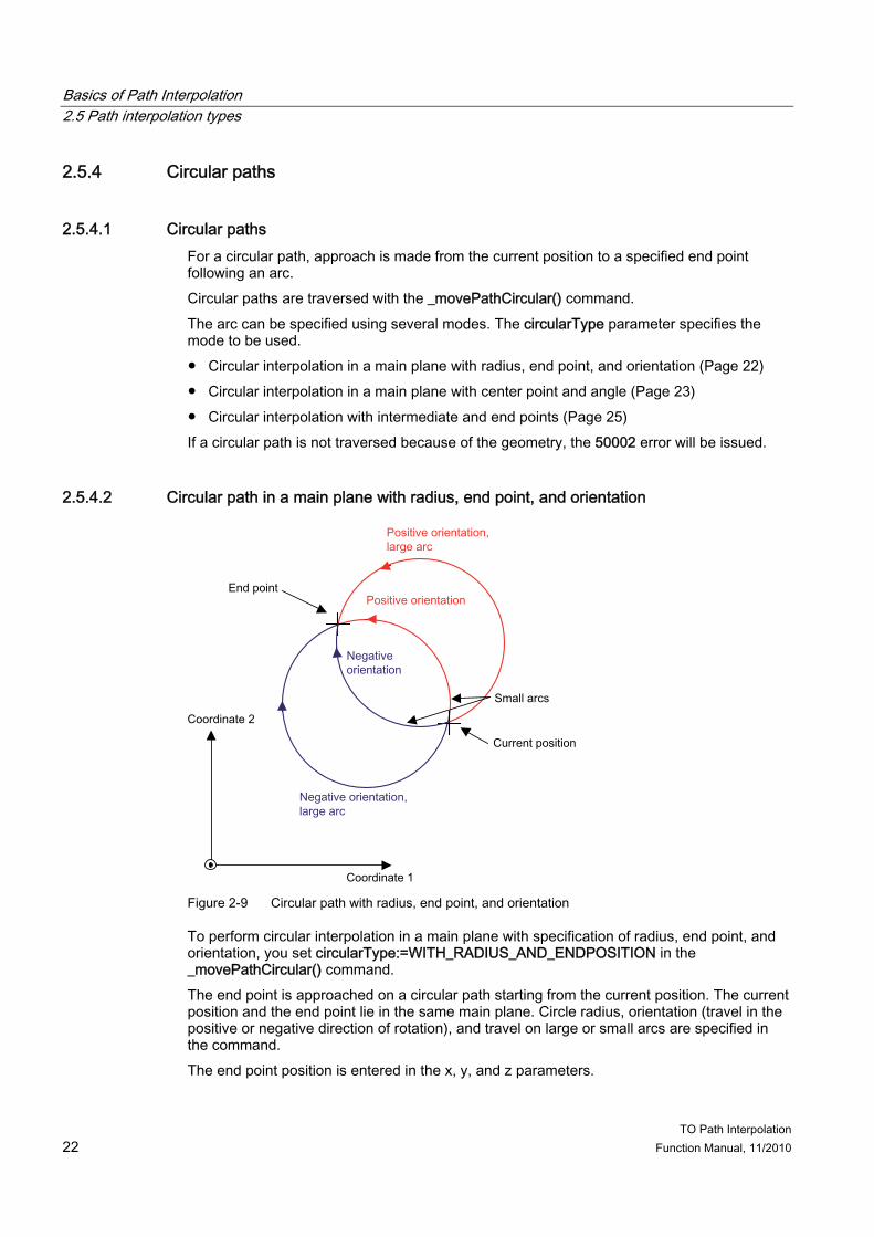
2.5.4.2 Circular path in a main plane with radius, end point, and orientation
Figure 2-9 Circular path with radius, end point, and orientation
To perform circular interpolation in a main plane with specification of radius, end point, and orientation, you set circularType:=WITH_RADIUS_AND_ENDPOSITION in the _movePathCircular() command. The end point is approached on a circular path starting from the current position. The current position and the end point lie in the same main plane. Circle radius, orientation (travel in the positive or negative direction of rotation), and travel on large or small arcs are specified in the command. The end point position is entered in the x, y, and z parameters.
Basics of Path Interpolation 2.5 Path interpolation types
TO Path Interpolation Function Manual, 11/2010 23
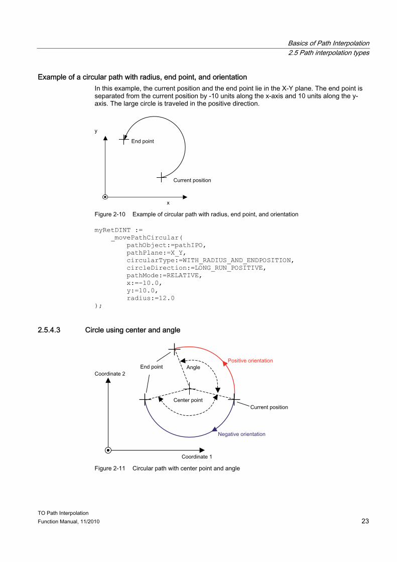
Example of a circular path with radius, end point, and orientation In this example, the current position and the end point lie in the X-Y plane. The end point is separated from the current position by -10 units along the x-axis and 10 units along the y-axis. The large circle is traveled in the positive direction.
Figure 2-10 Example of circular path with radius, end point, and orientation
Figure 2-11 Circular path with center point and angle
Basics of Path Interpolation 2.5 Path interpolation types
TO Path Interpolation 24 Function Manual, 11/2010
To perform circular interpolation starting from the current position in a main plane with specification of center point and angle, you set circularType:= BY_CENTER_AND_ARC in the _movePathCircular() command. The center point of the circle, the angle to be traveled, and the orientation (travel in the positive or negative direction of rotation) are specified in the command. The position of the center point of the circle is entered in the i, j, and k parameters. You use the ijkMode parameter to set whether the circle center point coordinates are entered absolutely or relative to the start point or whether the setting in the pathMode parameter should be used.
Example of a circular path with center point and angle In this example, the center point is separated by -10 units from the current position along the X-axis. An angle of 90 degrees in the positive direction is traveled.
Figure 2-12 Example of a circular path with center point and angle
Basics of Path Interpolation 2.5 Path interpolation types
TO Path Interpolation Function Manual, 11/2010 25
2.5.4.4 Circular path using intermediate point and end point
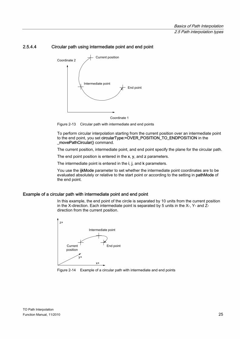
Figure 2-13 Circular path with intermediate and end points
To perform circular interpolation starting from the current position over an intermediate point to the end point, you set circularType:=OVER_POSITION_TO_ENDPOSITION in the _movePathCircular() command. The current position, intermediate point, and end point specify the plane for the circular path. The end point position is entered in the x, y, and z parameters. The intermediate point is entered in the i, j, and k parameters. You use the ijkMode parameter to set whether the intermediate point coordinates are to be evaluated absolutely or relative to the start point or according to the setting in pathMode of the end point.
Example of a circular path with intermediate point and end point In this example, the end point of the circle is separated by 10 units from the current position in the X-direction. Each intermediate point is separated by 5 units in the X-, Y- and Z-direction from the current position.
Figure 2-14 Example of a circular path with intermediate and end points
Basics of Path Interpolation 2.5 Path interpolation types
2.5.5.1 Polynomial paths A polynomial segment enables you to achieve a constant-velocity and constant-acceleration transition between two geometry elements and to make use of user-programmable curve shapes, e.g. from a higher-level CAD system. In addition to the implicit start point (PS) of the polynomial, the end point (PE) as well as four three-dimensional vectors for defining the polynomial coefficients are specified in the command parameters of the _movePathPolynomial() command The vectors are entered in the command using their components. Thus, for example, vector1 is entered with command parameters vector1x, vector1y, and vector1z. The polynomial can be defined in three ways: ● Direct specification of the polynomial coefficients (Page 28) ● Explicit specification of starting point data (Page 28) ● Attach continuously (Page 30) For the two explicit specification of the start point data and attach continuously types, the derivatives at the start and end points of the polynomial are required. They can be determined using integrated functions.
dds
d ds
2
2
Figure 2-15 Polynomial description by specification of the geometric derivatives
Basics of Path Interpolation 2.5 Path interpolation types
TO Path Interpolation Function Manual, 11/2010 27
Smooth-path transition between two linear paths
⎟⎟⎟
⎠
⎞
⎜⎜⎜
⎝
⎛ ⎟⎟⎟
⎠
⎞
⎜⎜⎜
⎝
⎛
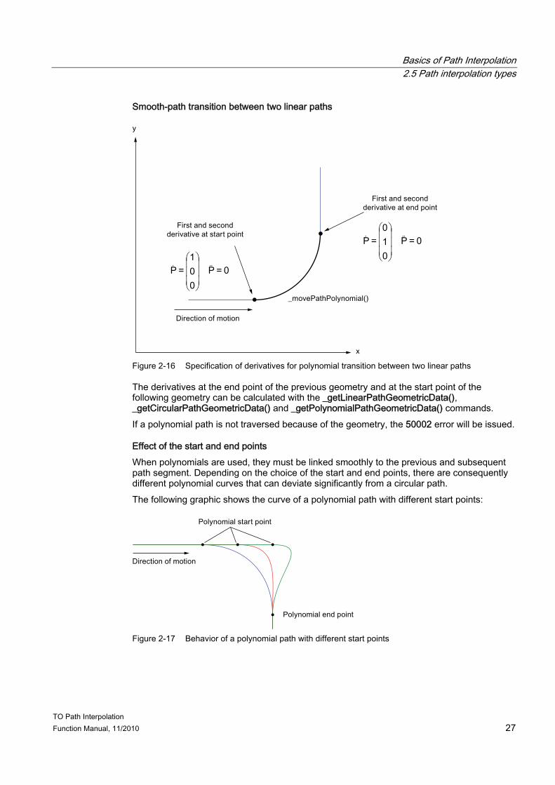
Figure 2-16 Specification of derivatives for polynomial transition between two linear paths
The derivatives at the end point of the previous geometry and at the start point of the following geometry can be calculated with the _getLinearPathGeometricData(), _getCircularPathGeometricData() and _getPolynomialPathGeometricData() commands. If a polynomial path is not traversed because of the geometry, the 50002 error will be issued.
Effect of the start and end points When polynomials are used, they must be linked smoothly to the previous and subsequent path segment. Depending on the choice of the start and end points, there are consequently different polynomial curves that can deviate significantly from a circular path. The following graphic shows the curve of a polynomial path with different start points:
Figure 2-17 Behavior of a polynomial path with different start points
Basics of Path Interpolation 2.5 Path interpolation types
TO Path Interpolation 28 Function Manual, 11/2010
2.5.5.2 Polynomial path - direct specification of the polynomial coefficients For the polynomial specification using (polynomialMode:=SETTING_OF_COEFFICIENTS() ) polynomial coefficients, the polynomial path is determined using a function of the fifth degree: P = A0 + A1 • p + A2 • p2 + A3 • p3 + A4 • p4 + A5 • p5 , p ∈ [0,1] ● vector1: A2 ● vector2: A3 ● vector3: A4 ● vector4: A5 ● A0 and A1 result from the start point and end point, and the predefined coefficients. For
the parameter area indicated above, this means: – A0 = start point – A1 = end point - start point - A2 - A3 - A4 - A5
2.5.5.3 Polynomial paths - explicit specification of the starting point data For the polynomialMode:=SPECIFIC_START_DATA setting and the explicit specification of the starting point data, the two geometric derivatives at the start point must also be specified for the derivatives at the end point of the polynomial. The derivatives must be specified as follows: ● vector1: First geometric derivative/tangential vector in start point ● vector2: Second geometric derivative/curvature vector in start point ● vector3: First geometric derivative/tangential vector in end point ● vector4: Second geometric derivative/curvature vector in end point
Example of a polynomial path with explicit specification of the starting point data This example connects a linear path and a circular path:
Figure 2-18 Example of a polynomial path with explicit specification of the starting point data
The two derivatives in the starting point of the polynomial must be calculated first. The _getLinearPathGeometricData() function used for this purpose calculates the two derivatives for the end point of the straight line (starting point of the polynomial) using the coordinates of the straight line.
Basics of Path Interpolation 2.5 Path interpolation types
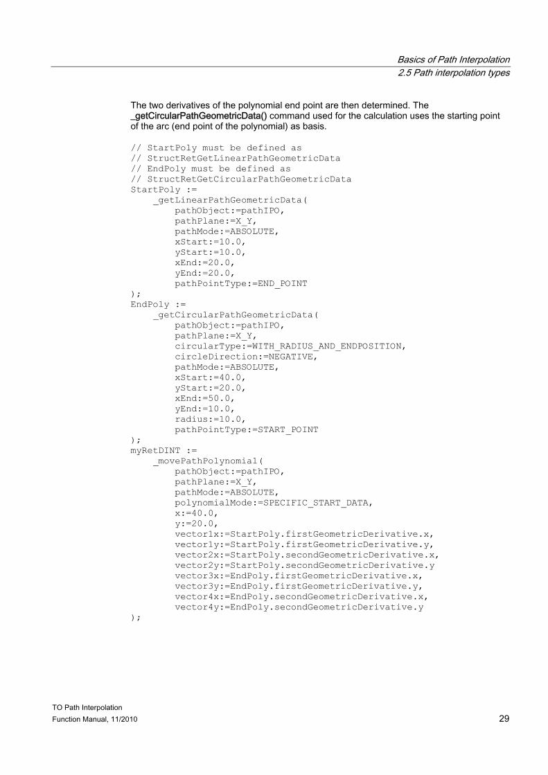
TO Path Interpolation Function Manual, 11/2010 29
The two derivatives of the polynomial end point are then determined. The _getCircularPathGeometricData() command used for the calculation uses the starting point of the arc (end point of the polynomial) as basis. // StartPoly must be defined as // StructRetGetLinearPathGeometricData // EndPoly must be defined as // StructRetGetCircularPathGeometricData StartPoly := _getLinearPathGeometricData( pathObject:=pathIPO, pathPlane:=X_Y, pathMode:=ABSOLUTE, xStart:=10.0, yStart:=10.0, xEnd:=20.0, yEnd:=20.0, pathPointType:=END_POINT ); EndPoly := _getCircularPathGeometricData( pathObject:=pathIPO, pathPlane:=X_Y, circularType:=WITH_RADIUS_AND_ENDPOSITION, circleDirection:=NEGATIVE, pathMode:=ABSOLUTE, xStart:=40.0, yStart:=20.0, xEnd:=50.0, yEnd:=10.0, radius:=10.0, pathPointType:=START_POINT ); myRetDINT := _movePathPolynomial( pathObject:=pathIPO, pathPlane:=X_Y, pathMode:=ABSOLUTE, polynomialMode:=SPECIFIC_START_DATA, x:=40.0, y:=20.0, vector1x:=StartPoly.firstGeometricDerivative.x, vector1y:=StartPoly.firstGeometricDerivative.y, vector2x:=StartPoly.secondGeometricDerivative.x, vector2y:=StartPoly.secondGeometricDerivative.y vector3x:=EndPoly.firstGeometricDerivative.x, vector3y:=EndPoly.firstGeometricDerivative.y, vector4x:=EndPoly.secondGeometricDerivative.x, vector4y:=EndPoly.secondGeometricDerivative.y );
Basics of Path Interpolation 2.5 Path interpolation types
TO Path Interpolation 30 Function Manual, 11/2010
2.5.5.4 Polynomial paths - attach continuously Polynomial paths can be attached continuously to a previous path segment using the polynomialMode:=ATTACHED_STEADILY setting. Because the geometric derivatives at the start point of the polynomial are taken from the predecessor geometry, only the first and the second derivative at the end point needs to be specified directly. The two derivatives for the polynomial command are specified as following: ● vector1: First geometric derivative/tangential vector in end point ● vector2: Second geometric derivative/curvature vector in end point If the geometric derivative cannot be determined in the start point (if no current motion is available), the command is not executed and error message 50002 "Calculation of the geometry element not possible, reason 3" is output.
Figure 2-19 Polynomial path - attach continuously
Example of a polynomial path attached continuously This example connects two straight lines using a polynomial.
Figure 2-20 Example for the continuous attachment of polynomial paths
The two derivatives at the end point of the polynomial must be calculated first. The _getLinearPathGeometricData() function used here returns a structure with the derivatives. The function calculates the derivatives for the start point of the straight lines (end point of the polynomial) using the start and end point coordinates of the straight lines. // EndPoly must be defined as // StructRetGetLinearPathGeometricData EndPoly := _getLinearPathGeometricData(
2.6.1 Path dynamics The path dynamics can be specified through preset dynamic values or a dynamic response profile. The dynamic limits of the individual axes for motion along the path can also be taken into consideration. An error message is output if the dynamic values are exceeded.
Figure 2-21 Path dynamics during path interpolation and dynamic limiting on the axis
Basics of Path Interpolation 2.6 Path dynamics
TO Path Interpolation 32 Function Manual, 11/2010
2.6.2 Preset path dynamics The path dynamics can be specified in two different ways in the respective motion command: ● Preset path dynamics via command parameters ● Preset path dynamics via velocity profile/cam
Preset path dynamics via command parameters The dynamic values (velocity, acceleration, and, if applicable, jerk) are explicitly specified in the velocity profile type. The path interpolator calculates the velocity profile for the path motion. Criteria for calculating the velocity profile include: ● The dynamic values for velocity, acceleration, and jerk specified in the path motion
command ● The type of velocity profile set in velocityProfile:
– TRAPEZOIDAL: Without jerk limitation; the path will be traveled with constant acceleration and deceleration.
– SMOOTH: With jerk limitation; the path will be traveled with smooth acceleration and deceleration curve.
Preset path dynamics via velocity profile/cam The path object can be interconnected with a cam for specifying a velocity profile. Velocity as well as the derived values for acceleration and, if applicable, jerk, are taken from the velocity profile. The base value (domain) is the path length. To rule out rounding errors in the path length calculation and to enable optimized calculation of profiles over more than one motion, parameters can be programmed simultaneously for the start and end points of the cam domain of the respective motion. At the command end, the dynamics specified in the profile are also applied to the motion. If additional follow-on motions are programmed, these dynamics are also applied to the transition to the new motion command. Possible settings for the path behavior at the motion end are ignored. If no additional follow-on motions are programmed or if the motion is to stop at the command end, the dynamics in the profile should be selected such that a stop at the motion end is possible; a velocity of 0 with a braking dynamic that can be achieved with certainty. In addition, the profile dynamics are limited by the dynamic values for the individual commands, taking into account the preassigned velocity profile type.
2.6.3 Limiting the path dynamics
Technological limiting The individual axis setpoints resulting from the path interpolation are limited to the dynamic limits specified for each path axis and positioning axis involved in path-synchronous motion.
Basics of Path Interpolation 2.6 Path dynamics
TO Path Interpolation Function Manual, 11/2010 33
The dynamic values of the axis for the path object are only taken into account if this has been programmed accordingly (command parameter blendingMode := ACTIVE_WITH_DYNAMIC_ADAPTION and/or dynamicAdaption <> INACTIVE). Path velocity limiting, path acceleration limiting, and path jerk limiting can be specified in the limitsOfPathDynamics system variables. Changes in the system variables take effect immediately. The maximum dynamic values over the path result from the lesser of the dynamic parameters set in the command, the dynamic limits on the path specified via the system variables (limitsOfPathDynamics), and, if programmed, the maximum dynamic values of the axes along the path. Note that the path velocity for active dynamic adaptation, possibly also reduced, if the dynamic limits of the axes would not be violated even without active dynamic adaptation. Because the reserve used for the active dynamic adaptation, the maximum possible dynamic path response will not always be attained.
Allowance for dynamic limits of path axes A reference to the dynamic limits of the axis can be established in the path object using the dynamicAdaption command parameter. The following settings are possible:
Basics of Path Interpolation 2.6 Path dynamics
TO Path Interpolation 34 Function Manual, 11/2010
● No allowance for maximum dynamic values of path axes (INACTIVE) With this setting, the axial limits are not taken into account within the path interpolation. However, path axis limiting is still active and, if a violation occurs, a setpoint-side path error can result. The setting is useful if: – There are no transformed dynamic values – It can be ensured in advance (e.g. during commissioning) that the axial limit values
are not exceeded – The axial limits have been taken into account through an application, e.g. through
calculation of an optimized velocity profile – Superimposed axis motions occur
● Reduction in the maximum path dynamics according to the maximum dynamic values of path axes (ACTIVE_WITH_CONSTANT_LIMITS) The velocity and acceleration of the path is limited in the path interpolator to the maximum values in the Cartesian coordinates calculated from the maximum value settings of the individual path axes. Axis-specific jerk limits in the preliminary path plan are not taken into account. However, the jerk can be limited by specifying the pathMotion monitoring on the path axis accordingly. This can result in a setpoint-side path error. If the dynamic limits of an axis are reached, i.e. if the programmed path velocity/acceleration cannot be achieved due to these limits, an alarm will be issued. If the dynamic limits of the path axes are changed online, the changes take effect immediately but not for the currently active or decoded motion command.
● Segment-by-segment reduction in the maximum path dynamics according to the maximum dynamic values of path axes in these segments (ACTIVE_WITH_VARIABLE_LIMITS). This setting is equivalent to ACTIVE_WITH_CONSTANT_LIMITS, except that the path is segmented. Overall, the path is travelled faster; the velocity is not constant over the entire path.
From system variable kinematicsData.transformationsOfDynamics of the path object, you can read out whether the maximum dynamic values of the axis are transformed values. If not, the path dynamics are always limited with the path object dynamic limits, regardless of the setting in the dynamicAdaption command parameter.
Difference between ACTIVE_WITH_CONSTANT_LIMITS and ACTIVE_WITH_VARIABLE_LIMITS The following trace shows the difference between ACTIVE_WITH_CONSTANT_LIMITS and ACTIVE_WITH_VARIABLE_LIMITS. Two circular paths are traveled with a 2D portal; the maximum velocities of the path axes follow: ● Axis_X: 500 mm/s ● Axis_Y: 200 mm/s A path velocity of 400 mm/s is defined in the path commands.
Basics of Path Interpolation 2.7 Stopping and resuming path motion
Override A velocity override (system variable override.velocity) and an acceleration override (system variable override.acceleration) are available on the path object.
2.7 Stopping and resuming path motion The _stopPath() command can be used to stop the current path motion. A stopped, but not canceled, path motion can be continued with the _continuePath() command. When the path motion is resumed, the motion properties (velocity profile, acceleration, etc.) of the interrupted path command are applied. With SIMOTION V4.2 and higher, other dynamism parameters can be specified directly at the command _continuePath(). In the case of canceled path motions, if you want the application to start at the abort position, the last calculated setpoint position on the path is indicated in the abortPosition system variable.
Dynamic response for _stopPath()
Basics of Path Interpolation 2.8 Path behavior at motion end
TO Path Interpolation 36 Function Manual, 11/2010
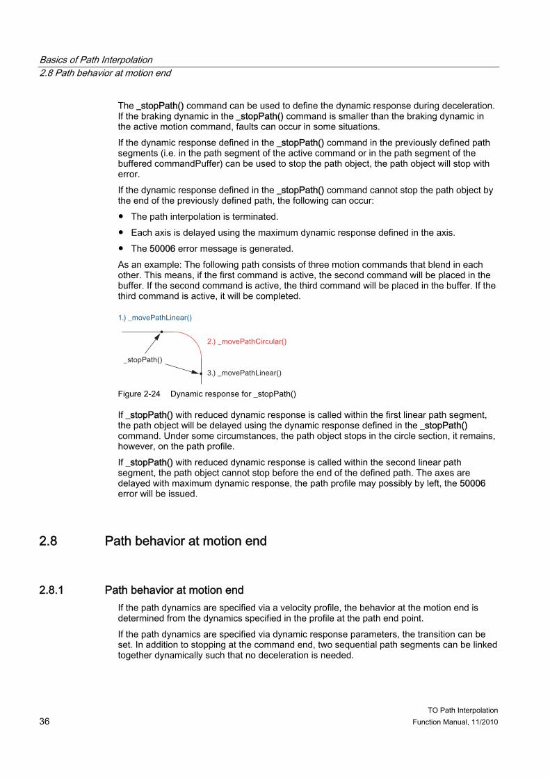
The _stopPath() command can be used to define the dynamic response during deceleration. If the braking dynamic in the _stopPath() command is smaller than the braking dynamic in the active motion command, faults can occur in some situations. If the dynamic response defined in the _stopPath() command in the previously defined path segments (i.e. in the path segment of the active command or in the path segment of the buffered commandPuffer) can be used to stop the path object, the path object will stop with error. If the dynamic response defined in the _stopPath() command cannot stop the path object by the end of the previously defined path, the following can occur: ● The path interpolation is terminated. ● Each axis is delayed using the maximum dynamic response defined in the axis. ● The 50006 error message is generated. As an example: The following path consists of three motion commands that blend in each other. This means, if the first command is active, the second command will be placed in the buffer. If the second command is active, the third command will be placed in the buffer. If the third command is active, it will be completed.
Figure 2-24 Dynamic response for _stopPath()
If _stopPath() with reduced dynamic response is called within the first linear path segment, the path object will be delayed using the dynamic response defined in the _stopPath() command. Under some circumstances, the path object stops in the circle section, it remains, however, on the path profile. If _stopPath() with reduced dynamic response is called within the second linear path segment, the path object cannot stop before the end of the defined path. The axes are delayed with maximum dynamic response, the path profile may possibly by left, the 50006 error will be issued.
2.8 Path behavior at motion end
2.8.1 Path behavior at motion end If the path dynamics are specified via a velocity profile, the behavior at the motion end is determined from the dynamics specified in the profile at the path end point. If the path dynamics are specified via dynamic response parameters, the transition can be set. In addition to stopping at the command end, two sequential path segments can be linked together dynamically such that no deceleration is needed.
Basics of Path Interpolation 2.8 Path behavior at motion end
TO Path Interpolation Function Manual, 11/2010 37
No intermediate segments for the fillet are generated by the path interpolation for this blending. Taking into account the axial limits, there are three transition types that can be set in the blendingMode parameter of the next command. ● Stopping at motion end (Page 37) (blendingMode:=INACTIVE) ● Blending with dynamic adaptation (Page 37)
(blendingMode:=ACTIVE_WITH_DYNAMIC_ADAPTION) ● Blending without dynamic adaptation (Page 38)
(blendingMode:=ACTIVE_WITHOUT_DYNAMIC_ADAPTION) The blendingMode parameter is only evaluated if the command is programmed with mergeMode:=SEQUENTIAL or mergeMode:=NEXT_MOTION. The blending mode is specified in the motion command in which blending is to be performed.
2.8.2 Stopping at motion end The motion is ended in the target position of the path command. The path velocity and acceleration is zero. Any new path motion becomes active only after END_OF_INTERPOLATION (end of setpoint generation).
2.8.3 Blending with dynamic adaptation During blending, the system supports a constant-velocity transition (with velocity profile type TRAPEZOIDAL) or a constant-velocity and constant-acceleration transition (with velocity profile type SMOOTH).
A C B
A
B C
Figure 2-25 Example of blending with dynamic adaptation: Straight line - straight line
With this setting, the dynamic limits of the axis are taken into account directly when calculating the travel profile for path blending. The axial limits for velocity and acceleration are also taken into account in the blending velocity. For non-tangential path transitions (corners), the path velocity is reduced such that a velocity jump greater than the maximum acceleration does not occur for any of the participating axes. The result is a velocity-dependent smoothing of the path end point.
Basics of Path Interpolation 2.9 Display and monitoring options on the axis
TO Path Interpolation 38 Function Manual, 11/2010
Note that with active dynamic adaptation, the dynamic axis response is set to the smaller value from axis acceleration and axis deceleration. Therefore, when an axis has a maximum acceleration of 1000 mm/s2 and a maximum deceleration of 500 mm/s2, the value for the deceleration is used for the calculation.
2.8.4 Blending without dynamic adaptation
A C B
A
B C
Figure 2-26 Example of blending without dynamic adaptation: Straight line - straight line
With this setting, the dynamic limits of the axis are not taken into account in path blending. The path velocity is controlled as a scalar variable that is independent of direction and curvature. A non-tangential attachment of path segments has no effect on the path velocity profile; for this reason, the velocity is not reduced during blending. Because the setpoints that are generated for the individual axes are limited to the axis-specific dynamic limits for the axes, this can result in an axis setpoint error relative to the setpoint from the path interpolation. This ultimately leads to an axis-specific deviation from the path in the blending range. For example, this mode is applicable if the dynamic limits of the axes are to be adhered to on the path (when approaching positions, for example) but an axis-specific axis setpoint error relative to the path is acceptable at the segment transitions in the blending range.
2.9 Display and monitoring options on the axis
Display and monitoring options for path motion on the axis An active path motion is indicated on the path axis in system variable pathMotion.state.
Display of path-synchronous motion on the positioning axis An active synchronous axis motion is indicated on the positioning axis in system variable pathSyncMotion.state.
Monitoring for setpoint error The path axis or positioning axis can be monitored for setpoint errors (discrepancy between the setpoint specified by the path object and the setpoint output on the axis). The difference between the setpoint and the actual value is not monitored.
Basics of Path Interpolation 2.10 Allowance for axis-specific traversing range limits
TO Path Interpolation Function Manual, 11/2010 39
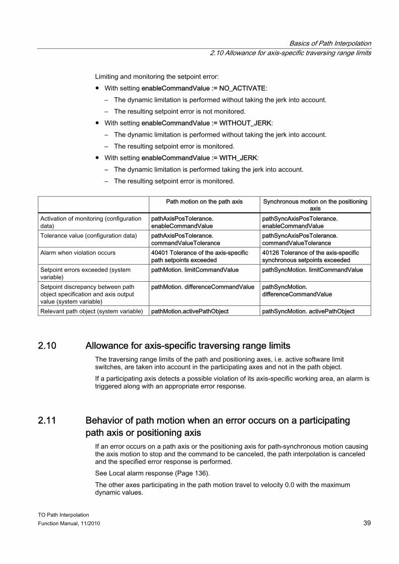
Limiting and monitoring the setpoint error: ● With setting enableCommandValue := NO_ACTIVATE:
– The dynamic limitation is performed without taking the jerk into account. – The resulting setpoint error is not monitored.
● With setting enableCommandValue := WITHOUT_JERK: – The dynamic limitation is performed without taking the jerk into account. – The resulting setpoint error is monitored.
● With setting enableCommandValue := WITH_JERK: – The dynamic limitation is performed taking the jerk into account. – The resulting setpoint error is monitored.
Path motion on the path axis Synchronous motion on the positioning
axis Activation of monitoring (configuration data)
pathAxisPosTolerance. enableCommandValue
pathSyncAxisPosTolerance. enableCommandValue
Tolerance value (configuration data) pathAxisPosTolerance. commandValueTolerance
pathSyncAxisPosTolerance. commandValueTolerance
Alarm when violation occurs 40401 Tolerance of the axis-specific path setpoints exceeded
40126 Tolerance of the axis-specific synchronous setpoints exceeded
2.10 Allowance for axis-specific traversing range limits The traversing range limits of the path and positioning axes, i.e. active software limit switches, are taken into account in the participating axes and not in the path object. If a participating axis detects a possible violation of its axis-specific working area, an alarm is triggered along with an appropriate error response.
2.11 Behavior of path motion when an error occurs on a participating path axis or positioning axis
If an error occurs on a path axis or the positioning axis for path-synchronous motion causing the axis motion to stop and the command to be canceled, the path interpolation is canceled and the specified error response is performed. See Local alarm response (Page 136). The other axes participating in the path motion travel to velocity 0.0 with the maximum dynamic values.
Basics of Path Interpolation 2.12 Functionality of path-synchronous motion
TO Path Interpolation 40 Function Manual, 11/2010
2.12 Functionality of path-synchronous motion
2.12.1 Functionality of path-synchronous motion A path-synchronous motion on a positioning axis can be specified synchronous to the path motion with which it is specified. This causes the path-synchronous motion to start and end at the same time as the path motion. This enables a gripper to rotate in synchronism with the path motion, for example. The path motion and the path-synchronous motion follow a common traversing profile. This also applies to the blending between two path segments.
2.12.2 Specification of path-synchronous motion There are several options for path-synchronous motion, which are specified in the wMode parameter of the respective motion command: ● Motion to a defined end point in the coordinate system of the positioning axis
The target position of the path-synchronous motion is specified in the path command. This can be a relative (RELATIVE) or absolute (ABSOLUTE) position. As for the positioning command of the axis, the direction of the synchronous motion is specified using a parameter (wDirection). For further information, refer to the Motion Control, TO axis, electrical / hydraulic, external encoder Function Manual, "Positioning". The motion dynamics conform to the path, and the axis is "carried along". If the maximum dynamic values of the positioning axis are thereby violated, the dynamic parameters of the path are reduced accordingly. If the path length is zero and a path-synchronous motion is programmed, an error will be issued and the path-synchronous motion set to the programmed end position. The resulting setpoint jump is traversed axially with the maximum values. In this case, it is important to note that a configured monitoring of the setpoint error of the synchronous axis also acts on the setpoint jump.
● Motion according to current path length The current path distance is output. There are two ways of doing this: – Reference to the command (OUTPUT_PATH_LENGTH)
The axis position is first set to 0.0 before the path distance is traveled. The reset of the axis position to zero is equivalent to a synchronized _redefinePosition() command.
– Accumulated output without reset (OUTPUT_PATH_LENGTH_ADDITIVE) The path distance accumulated via the command limit is output.
Basics of Path Interpolation 2.12 Functionality of path-synchronous motion
TO Path Interpolation Function Manual, 11/2010 41
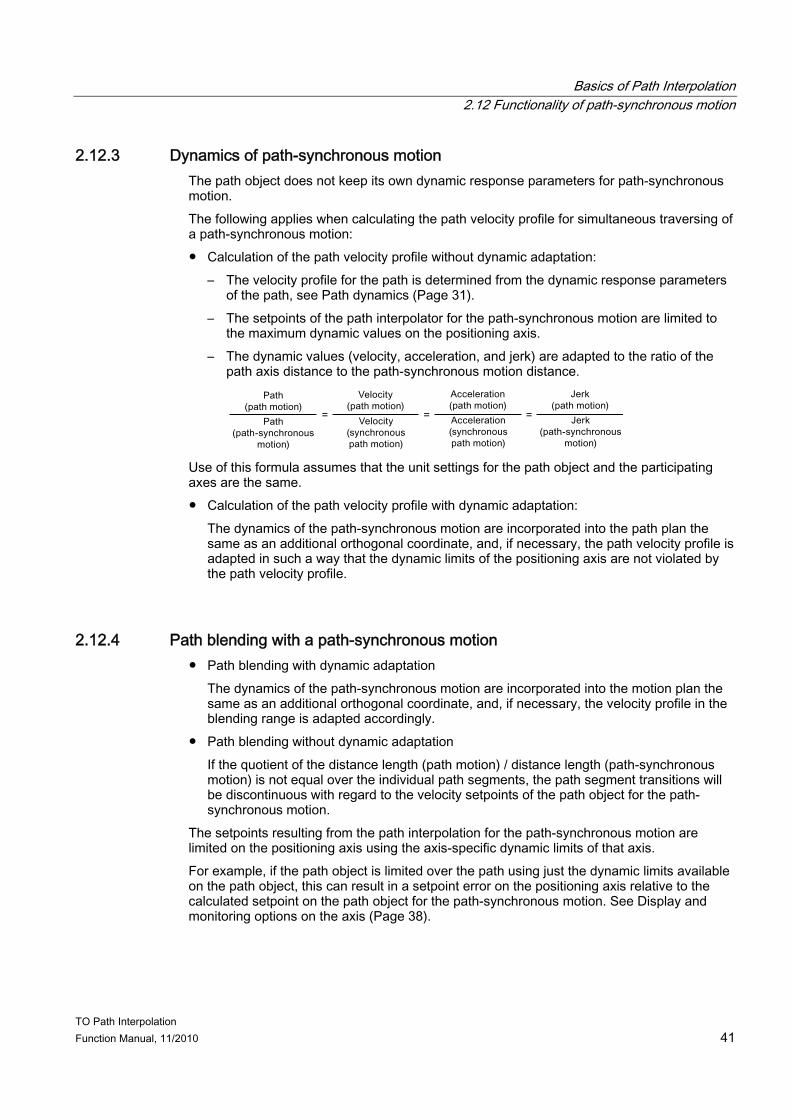
2.12.3 Dynamics of path-synchronous motion The path object does not keep its own dynamic response parameters for path-synchronous motion. The following applies when calculating the path velocity profile for simultaneous traversing of a path-synchronous motion: ● Calculation of the path velocity profile without dynamic adaptation:
– The velocity profile for the path is determined from the dynamic response parameters of the path, see Path dynamics (Page 31).
– The setpoints of the path interpolator for the path-synchronous motion are limited to the maximum dynamic values on the positioning axis.
– The dynamic values (velocity, acceleration, and jerk) are adapted to the ratio of the path axis distance to the path-synchronous motion distance.
Use of this formula assumes that the unit settings for the path object and the participating axes are the same. ● Calculation of the path velocity profile with dynamic adaptation:
The dynamics of the path-synchronous motion are incorporated into the path plan the same as an additional orthogonal coordinate, and, if necessary, the path velocity profile is adapted in such a way that the dynamic limits of the positioning axis are not violated by the path velocity profile.
2.12.4 Path blending with a path-synchronous motion ● Path blending with dynamic adaptation
The dynamics of the path-synchronous motion are incorporated into the motion plan the same as an additional orthogonal coordinate, and, if necessary, the velocity profile in the blending range is adapted accordingly.
● Path blending without dynamic adaptation If the quotient of the distance length (path motion) / distance length (path-synchronous motion) is not equal over the individual path segments, the path segment transitions will be discontinuous with regard to the velocity setpoints of the path object for the path-synchronous motion.
The setpoints resulting from the path interpolation for the path-synchronous motion are limited on the positioning axis using the axis-specific dynamic limits of that axis. For example, if the path object is limited over the path using just the dynamic limits available on the path object, this can result in a setpoint error on the positioning axis relative to the calculated setpoint on the path object for the path-synchronous motion. See Display and monitoring options on the axis (Page 38).
Basics of Path Interpolation 2.13 Kinematic adaptation
TO Path Interpolation 42 Function Manual, 11/2010
2.12.5 Output of the path distance to the positioning axis Alternatively, the traveled path distance, i.e. the current path length, can be output to the positioning axis. This distance can be relative to an individual path segment or added up over multiple path segments. The setting is made in the path command. For example, this can be used to output path distance-related output cams or measuring inputs.
2.12.6 Output of Cartesian coordinates using the MotionOut Interface The motionOut.x/y/z interfaces can be used to interconnect the Cartesian coordinates directly with other technology objects, e.g. with the MotionIn interfaces of positioning axes. For example, this functionality can be used in the application to implement output cams and measuring inputs on Cartesian axes.
2.13 Kinematic adaptation
2.13.1 Kinematic adaptation The kinematic transformation or the kinematic adaptation is used to convert path axis values to the Cartesian axes, and vice versa.
2.13.2 Kinematic adaptation – fundamentals
2.13.2.1 Scope of the transformation functionality During forward calculation of the kinematics (including direct kinematics, forward kinematics or forward transformation) for position and motion conversion, the position of the end point of the kinematics is determined in the basic coordinate system from the position of the articulation angle and its spatial arrangement. During backward calculation (including backward transformation or inverse kinematics), the position of the individual articulation angle is determined from the position of the end point of the kinematics in the basic coordinate system. For path interpolation, the position of the end point of the kinematics in the basic coordinate system is calculated over time. The position and the dynamic values are transformed. The current modulo range is retained in path axes specified as modulo axes. See Modulo properties (Page 17).
Basics of Path Interpolation 2.13 Kinematic adaptation
TO Path Interpolation Function Manual, 11/2010 43
2.13.2.2 Reference points The following reference points are used in path interpolation: ● Cartesian zero point ● Kinematic zero point ● Kinematic end point
(because a tool is not taken into account, this is equal to the path point)
Figure 2-27 Reference points of the coordinate systems in path interpolation
The path object calculates the position on the path. This is also the kinematic end point.
2.13.2.3 System variables for path interpolation and transformation on the path object
Figure 2-28 Overview of system variables of the path object
The position values and dynamic values can be accessed via a system variable:
Path data System variables Description path.acceleration Path acceleration path.command Status of a motion command path.dynamicAdaption Indicator that maximum dynamic values of
path axes are being taken into account path.length Length of the current path
Basics of Path Interpolation 2.13 Kinematic adaptation
TO Path Interpolation 44 Function Manual, 11/2010
System variables Description path.motionState Motion status of path motion path.position Path position (within the path length) path.velocity Path velocity
Cartesian specifications in the basic coordinate system / path-synchronous motion System variables Description bcs.x/y/z/w.position Set positions bcs.x/y/z/w.velocity Set velocities bcs.x/y/z/w.acceleration Set accelerations bcs.linkConstellation Set link constellation
Cartesian actual values System variables Description bcs.x/y/zActual.position Actual value of the Cartesian positions of the
path axes bcs.linkConstellationActual Current link constellation
Defaults on path axes from path motion System variables Description mcs.a1/a2/a3.acceleration Accelerations of the path axes mcs.a1/a2/a3.position Positions of path axes in the axis coordinates mcs.a1/a2/a3.velocity Velocities of the path axes
Object coordinate system System variables Description ocs[1..3].trackingIn Interface for motion sequence reference
value with which the OCS is to be coupled (e.g. TO external encoder)
ocs[1..3].trackingInPosition Current value of the motion sequence ocs[1..3].trackingPosition Position of the OCS relative to the reference
position ocs[1..3].trackingState Synchronization status ocs[1..3].x/y/z.accelaration Acceleration ocs[1..3].x/y/z.position Item ocs[1..3].x/y/z.velocity Velocity
Override
Basics of Path Interpolation 2.13 Kinematic adaptation
TO Path Interpolation Function Manual, 11/2010 45
System variables Description override.acceleration Acceleration override override.velocity Velocity override
Path command statuses System variables Description linearPathCommand.state Status of linear interpolation circularPathCommand.state Status of circular interpolation polynomialPathCommand.state Status of polynomial interpolation
2.13.2.4 Transformation of the dynamic values The kinematicsData.transformationOfDynamics system variable indicates whether a kinematic transformation supports the dynamics transformation functionality.
2.13.2.5 Differentiation of link constellations If Cartesian kinematics end points can be reached via various articulation positions, articulation positioning spaces are defined for the corresponding kinematics. All path motions take place in the same link constellation. For this reason, a change to another link constellation is not possible when a path is being executed. A change to another link constellation is possible through individual axis motions but not via a motion on the path object. The current transformation-specific link constellation is indicated on the setpoint side in the bcs.linkConstellation variable and on the actual value side in the bcs.linkConstellationActual variable. The link constellation is defined specifically for each transformation. See Supported kinematics (Page 48).
2.13.2.6 Information commands for the kinematic transformation In addition to the implicit conversion in the system, the transformation calculations can also be accessed directly via user commands. ● The _getPathCartesianPosition() command is used to calculate the Cartesian positions
for the axis positions specified in the command. ● The _getPathAxesPosition() command is used to calculate the axis positions from the
Cartesian positions. ● The _getPathCartesianData() command is used to calculate the Cartesian data for the
position, velocity, and acceleration from the axis positions, axis velocities, and axis accelerations specified in the command.
● The _getPathAxesData() command is used to calculate the axis positions, axis velocities, and axis accelerations from the Cartesian data for the position, velocity, and acceleration specified in the command.
Basics of Path Interpolation 2.13 Kinematic adaptation
TO Path Interpolation 46 Function Manual, 11/2010
For the calculation of axis positions, the values are specified in the axis coordinate of the path axis, and not relative to the kinematic zero point of the axis. The modulo range is taken into account. For the transformation of Cartesian values to path axis values, a link constellation and not a reference position of the axes has to be specified in order to ensure uniqueness.
2.13.2.7 Axis-specific zero point offset in the transformation It is possible to set an axis-specific offset of the zero position of the axis in the axis-specific coordinate system as well as the zero definition of the axis in the transformation. The positive direction of the axis and of the axis in the transformation must be the same. These settings are made for the axis. The offset of the kinematic zero point relative to the axis zero point is specified in the positive direction of the axis.
Figure 2-29 Path axis offset
When modulo axes are used for rotary links with a limited domain in kinematics, such as SCARA, the axis-specific zero point offset and the modulo property of the relevant path axis are defined such that the permissible modulo range of the path axis coincides with the domain of the relevant arm within the kinematics. Otherwise, this can cause an additional limitation in the traversing range of the kinematics. Example: If a link is limited to [-180°; 180°) and a modulo range of 0° to 360° is defined on the path axis, the zero point offset to -180° should be specified.
Basics of Path Interpolation 2.13 Kinematic adaptation
TO Path Interpolation Function Manual, 11/2010 47
2.13.2.8 Offset of the kinematic zero point relative to the Cartesian zero point An offset of the kinematic zero point of the transformation relative to the Cartesian zero point can be set in the basicOffset configuration data.
A 1
A 2
basicOffset
A 3
x+
z+
y+
Figure 2-30 Example of kinematic offset
The above example produces negative values for the kinematic offsets. Offset in example: x: -100 y: -100 z: -200 With SIMOTION V4.2 and higher, not only can the BCS be offset but also rotated, allowing for any rotation of the coordinate system from the kinematics zero point. This allows flexible assignment of the BCS to the handling equipment's kinematics.
Figure 2-31 Coordinate system offset and rotation
The rotations are undertaken after the offset in the following order: 1. Roll around x axis 2. Pitch around (already rotated) y axis 3. Yaw around (already twice rotated) z axis
Basics of Path Interpolation 2.13 Kinematic adaptation
TO Path Interpolation 48 Function Manual, 11/2010
A1
A2
basicOffset
A3
x+
z+
y+
Figure 2-32 Example of kinematics offset with rotation
Offset and rotation (around the y axis) in the example: x: -100 y: -100 z: -200 roll: 0° pitch: +15° jaw: 0°
2.13.3 Supported kinematics
2.13.3.1 Supported kinematics and their assignment The following kinematics can be set using the typeOfKinematics configuration data: ● Cartesian 2D/3D gantries (Page 51) (CARTESIAN): ● Picker kinematics:
● SCARA kinematics (Page 58) (SCARA) ● Articulated arm kinematics (Page 61) (ARTICULATED_ARM) ● 2-axis articulated arm kinematics (Page 64) (ARTICULATED_ARM_2D) available from
V4.2. ● Swivel arm kinematics (Page 65) (SWIVEL_ARM) available from V4.2. ● Other special kinematics (Page 68).(SPECIFIC) A transformation can be selected for each path object. Thus, multiple transformations can be configured/active in a SIMOTION system when multiple path objects are used.
Basics of Path Interpolation 2.13 Kinematic adaptation
TO Path Interpolation Function Manual, 11/2010 49
Because a path axis can be interconnected with more than one path object, a path axis can theoretically be involved in multiple kinematic assemblies but obviously can only be active in one path group at a time.
2.13.3.2 Configuration screens With SIMOTION version 4.2 and higher you can use parameterization screens to configure the kinematics. You can access the screens via the configuration menu.
Figure 2-33 Open configuration
Depending on the kinematics, the screen will contain several tabs where you can enter mechanical data and offsets and rotations.
Basics of Path Interpolation 2.13 Kinematic adaptation
TO Path Interpolation 50 Function Manual, 11/2010
Figure 2-35 Cartesian kinematics 2D - offset
Basics of Path Interpolation 2.13 Kinematic adaptation
TO Path Interpolation Function Manual, 11/2010 51
2.13.3.3 Cartesian 2D/3D gantries
basicOffset
Figure 2-36 Kinematics example: 2D/3D gantry
Configuration data for Cartesian kinematics typeOfKinematics: CARTESIAN
Cartesian gantry kinematic type
BasicOffset.x Offset of the zero point of Cartesian coordinate x relative to the zero point of axis coordinate A1
BasicOffset.y Offset of the zero point of Cartesian coordinate y relative to the zero point of axis coordinate A2
BasicOffset.z Offset of the zero point of Cartesian coordinate z relative to the zero point of axis coordinate A3
cartesianKinematicsType Select 2D or 3D (determines the number of axes involved)config2D Main plane (only for 2D gantry)
Possible link constellations linkConstellation Irrelevant (always 1)
Basics of Path Interpolation 2.13 Kinematic adaptation
TO Path Interpolation 52 Function Manual, 11/2010
2.13.3.4 Roller picker
Figure 2-37 Roller picker: Representation of the axis system
The roller picker has two-dimensional kinematics. You can configure roller pickers in all three main planes. This description assumes a configuration in the X-Y plane.
x I +
y I +
(R 1I , φ 1I ) (R 2I , φ 2I )
Figure 2-38 Kinematics of roller picker (deflection roll on the opposite side of the tool)
The deflection roll must be located on the opposite side of the tool.
Basics of Path Interpolation 2.13 Kinematic adaptation
TO Path Interpolation Function Manual, 11/2010 53
x II +
y II +
(R 1II ,φ 1II (R 2II , φ 2II )
Figure 2-39 Kinematics of roller picker (deflection roll on the tool; this case is not examined here)
The alternative variant with the deflection role on the tool can be derived by converting the coordinates: Deflection role on the tool Deflection role on the opposite side of the toolxII* -xI yII* -yI φ1II* φ 2I φ 2II* φ 1I R1II* R2I R2II* R1I
Note The two path axes must be configured so that 360 axis-units (i.e. mm, degree, etc.) produce a disk revolution. The "modulo axis" setting should be prevented. See Units (Page 18) and Modulo properties (Page 17).
Configuration data for roller picker kinematics typeOfKinematics: ROLL_PICKER Roller picker kinematics type basicOffset.x Offset of the kinematic zero point relative to the
Cartesian zero point, x-coordinate basicOffset.y Offset of the kinematic zero point relative to the
Cartesian zero point, y-coordinate Axis 3 is not available for the roller picker. config2D Main plane of the path axes
Basics of Path Interpolation 2.13 Kinematic adaptation
TO Path Interpolation 54 Function Manual, 11/2010
Specification of the radius of the disks on the motors in: radius1 Disk radius for path axis 1 radius2 Disk radius for path axis 2
Possible link constellations LinkConstellation Irrelevant (always 1)
2.13.3.5 Delta 2D picker
G1 G2
G3 G4
x+
y+
Figure 2-40 Kinematics of Delta 2D picker (X-Y plane example)
Definitions ● The complete structure is contained in one of the two-dimensional main planes. The X-Y
plane is used as an example in the following description. ● A1 and A2 designate the two active drive axes of the kinematic structure. They lie on the
straight line y = 0 and are separated from each other by the distance 2x distanceD1. Their zero position within the kinematic structure corresponds to the orientation of the upper arm segments (length1) in the direction of the negative Y axis. Positive displacements occur as shown in the figure.
● It is assumed that always a horizontal orientation of the lower connection plate between G3 and G4 occurs. This produces yG3 = yG4 and a horizontal separation of 2x distanceD2.
● When xZP = yZP = 0, the zero position of the kinematics lies in the center between drive axes A1 and A2.
● The end point of the direct transformation is defined with its coordinates xEP and yEP in the center between G3 and G4. This yields the position for G3 = (xEP-distanceD2; yEP) as well as G4 = (xEP+distanceD2; yEP).
Basics of Path Interpolation 2.13 Kinematic adaptation
TO Path Interpolation Function Manual, 11/2010 55
Configuration data for Delta 2D picker kinematics typeOfKinematics: DELTA_2D_PICKER
Delta 2D picker kinematics type
basicOffset Offset of the kinematic zero point (ZP) relative to a Cartesian zero point
basicOffset.x Portion of offset in coordinate direction X basicOffset.y Portion of offset in coordinate direction Y Axis 3 is not available for the Delta-2D picker. config2D Main plane of the path axes length1 Length of the upper arm segment length2 Length of the lower arm segment distanceD1 Distance of the A1 and A2 drive axes from the kinematic
zero point (ZP) distanceD2 Distance of the G3 and G4 articulations from the end
point (EP) offsetA1 Offset of the A1 drive axis offsetA2 Offset of the A2 drive axis
Possible link constellations LinkConstellation Irrelevant (always 1)
2.13.3.6 Delta 3D picker
x+
y+
G1
G2
length1
length1
length1
distanceD1
G3
Figure 2-41 Kinematics of Delta 3D picker (top view)
Basics of Path Interpolation 2.13 Kinematic adaptation
TO Path Interpolation 56 Function Manual, 11/2010
x+
y+
G1
G2
G3
G6
G4G5
Figure 2-42 Kinematics of Delta 3D picker (bottom view)
G4
G1
x
z+
Figure 2-43 Kinematics of the Delta 3D picker (single arm on the example, axis A1)
Definitions ● A1, A2, and A3 designate the three active drive axes of the kinematic structure. They lie in
the X-Y plane with z = 0, and each has distance d1 from the kinematic zero point (ZP). Their zero position within the kinematic structure corresponds to the direct orientation of the upper arm segments (length1) in the direction of the negative Z axis. Positive displacements occur counterclockwise, as shown in the previous figure.
● G1 to G6 identify freely movable links. ● It is assumed that the connection of the links at the end point (EP) has a horizontal
orientation based on the parallel struts. This yields yG4 = yG5 = yG6. G4 to G6 each have the horizontal separation distanceD2 from the end point (EP).
Basics of Path Interpolation 2.13 Kinematic adaptation
TO Path Interpolation Function Manual, 11/2010 57
● When xZP = yZP = zZP = 0, the zero position of the kinematics lies in the center between drive axes A1 and A3.
● The end point of the transformation is defined with its coordinates xEP, yEP and zEP centrally between G4 to G6.
Configuration data for Delta 3D picker kinematics typeOfKinematics: DELTA_3D_PICKER
Delta 3D picker kinematics type
basicOffset Offset of the kinematic zero point (ZP) relative to a Cartesian zero point
basicOffset.x Portion of offset in coordinate direction X basicOffset.y Portion of offset in coordinate direction Y basicOffset.z Portion of offset in coordinate direction Z length1 Length of the upper arm segment length2 Length of the lower arm segment distanceD1 Distance of the A1 to A3 drive axes from the kinematic
zero point (ZP) distanceD2 Distance of the G4 to G6 articulations from the end point
(EP) offsetA1 Offset of the drive axis A1 offsetA2 Offset of the drive axis A2 offsetA3 Offset of the drive axis A3 angleArm1ToX Angle offset of arm A1-G1-G4 from the X axis during
rotation at the positive Z axis angleArm2ToArm1 Angle offset of arm A2-G2-G5 from arm A1-G1-G4 during
rotation at the positive Z axis angleArm3ToArm1 Angle offset of arm A3-G3-G6 from arm A1-G1-G4 during
rotation at the positive Z axis
Possible link constellations LinkConstellation Irrelevant (always 1)
Basics of Path Interpolation 2.13 Kinematic adaptation
TO Path Interpolation 58 Function Manual, 11/2010
2.13.3.7 SCARA kinematics
Figure 2-44 SCARA: Representation of the axis system
A 3
A 1 A 2 EP
dx,y,z
d A1A2 d A2EP
x+ y+
z+
Figure 2-45 SCARA: Kinematics
The kinematic zero point lies in point A1.
Basics of Path Interpolation 2.13 Kinematic adaptation
TO Path Interpolation Function Manual, 11/2010 59
The zero positions of the A1 axis and A2 axis are as follows:
Figure 2-46 SCARA: Zero positions
The domain of the single A1 and A2 axes is limited to [-180°; 180°).
Link compensations
A 1 A 2
EP
d A1A2
d x,y,z
A 4
d A2EP
AP
A 3
x+ y+
z+
Figure 2-47 SCARA: Kinematics with link compensation
Coupled axes Mechanical couplings can exist: ● Between A1 and A2 ● Between A1, A2 and Asynchronous (A4) ● Between Asynchronous (A4) and A3 If a positive coupling factor between two axes is specified, the transformation assumes that a positive motion on the first axes leads to a negative motion on the second axis. The following axis couplings can be compensated via the system:
Basics of Path Interpolation 2.13 Kinematic adaptation
TO Path Interpolation 60 Function Manual, 11/2010
● A coupling from axis A1 to axis A2 ● A coupling from axis A1 and axis A2 to the path-synchronous controlled axis A4
That is, the setpoint of axis A4 is changed to the positioning axis in accordance with the changes of A1 and A2. If axis A1 and/or axis A2 is traversed and a path-synchronous motion on axis A4 is specified in parallel, the system superimposes/adds a path-synchronous motion specification and compensation onto the positioning axis.
● A coupling from axis A4 to axis A3 (lifting axis) If axis A3 is traversed via the path motion and a compensation from axis A4 to axis A3 is required simultaneously, the specifications are superimposed.
The compensation functionality and the specifications to the positioning axis A4 via the path-synchronous motion are independent of one another and are executed simultaneously by the system.
Configuration data for SCARA kinematics typeOfKinematics: SCARA SCARA kinematics type basicOffset.x Offset of the kinematic zero point relative to the
Cartesian zero point, x-coordinate basicOffset.y Offset of the kinematic zero point relative to the
Cartesian zero point, y-coordinate basicOffset.z Offset of the kinematic zero point relative to the
Cartesian zero point, z-coordinate offsetA1 Offset of axis zero point axis A1 relative to zero position
of axis A1 in the transformation distanceA1A2 A1-A2 separation offsetA2 Offset of axis zero point axis A2 relative to zero position
of axis A2 in the transformation distanceA2Endpoint A2 - end point separation linkCompensationA2.enableA1A2 Compensate A1 articulated joint positioning dependence
Basics of Path Interpolation 2.13 Kinematic adaptation
TO Path Interpolation Function Manual, 11/2010 61
Possible link constellations LinkConstellation 1 Positive link position: angle of axis A2 in the range
of [0°, 180°) relative to the kinematic zero point 2 Negative link position: Angle of axis A2 in the
range of [-180°, 0°) relative to the kinematic zero point
Figure 2-48 Possible link positions
2.13.3.8 Articulated arm kinematics
Figure 2-49 Articulated arm: Representation of the axes
Basics of Path Interpolation 2.13 Kinematic adaptation
TO Path Interpolation 62 Function Manual, 11/2010
Figure 2-50 Articulated arm: Kinematics
The kinematic zero point lies in point A1. The zero position of the kinematics exists if distanceA1A2, distanceA2A3 and distanceA3EP point in the Cartesian x-direction.
Figure 2-51 Articulated arm: Axes A2 and A3 zero positions
Basics of Path Interpolation 2.13 Kinematic adaptation
TO Path Interpolation Function Manual, 11/2010 63
Figure 2-52 Articulated arm: Axis A1 zero position
The domain of the single A1 to A3 axes is limited to [-180°; 180°).
Coupled axes If a positive coupling factor between two axes is specified, the transformation assumes that a positive motion on the first axes leads to a negative motion on the second axis.
Configuration data for articulated arm kinematics typeOfKinematics: ARTICULATED_ARM
Articulated arm kinematics type
basicOffset.x Offset of the kinematic zero point relative to the Cartesian zero point, x-coordinate
basicOffset.y Offset of the kinematic zero point relative to the Cartesian zero point, y-coordinate
basicOffset.z Offset of the kinematic zero point relative to the Cartesian zero point, z-coordinate
offsetA1 Offset of axis zero point axis A1 relative to zero position of axis A1 in the transformation
distanceA1A2 A1-A2 separation offsetA2 Offset of axis zero point axis A2 relative to zero position
of axis A2 in the transformation distanceA2A3 A2 - A3 separation offsetA3 Offset of axis zero point axis A3 relative to zero position
of axis A3 in the transformation distanceA3Endpoint A3 - end point separation linkCompensation.enableA2A3 Compensate A3 articulated joint positioning dependence
for A2 linkCompensation.factorA2A3 Factor
Basics of Path Interpolation 2.13 Kinematic adaptation
TO Path Interpolation 64 Function Manual, 11/2010
Possible link constellations LinkConstellation 1 Angle of axis A3 in the range of [0°, 180°) relative
to the kinematic zero point Angle of axis A1 corresponds to atan(EPy/EPx)
2 Angle of axis A3 in the range of [-180°, 0°) relative to the kinematic zero point Angle of axis A1 corresponds to atan(EPy/EPx)
3 Angle of axis A3 in the range of [0°, 180°) relative to the kinematic zero point Angle of axis A1 corresponds to –atan(EPy/EPx)
4 Angle of axis A3 in the range of [-180°, 0°) relative to the kinematic zero point Angle of axis A1 corresponds to –atan(EPy/EPx)
2.13.3.9 2axis articulated arm kinematics
2axis articulated arm kinematics
Figure 2-53 Display of the axes
Basics of Path Interpolation 2.13 Kinematic adaptation
TO Path Interpolation Function Manual, 11/2010 65
Table 2- 1 Configuration data for 2-axis articulated arm kinematics
typeOfKinematics:ARTICULATED_ARM_2D 2axis articulated arm kinematics type of kinematics
basicOffset.x Offset of the kinematic zero point relative to the Cartesian zero point, x coordinate
basicOffset.y Offset of the kinematic zero point relative to the Cartesian zero point, y coordinate
basicOffset.z Offset of the kinematic zero point relative to the Cartesian zero point, z coordinate
basicOffset.roll Offset axis zero of X axis basicOffset.pitch Offset axis zero of Y axis basicOffset.yaw Offset axis zero of Z axis Config2D Main plane of the path axes linkCompensationA2.enableA1A2 Compensate A1 articulated joint positioning
Swivel arm In swivel arm kinetics, programming settings are made on the lateral surface that can be accessed by the kinematics.
Basics of Path Interpolation 2.13 Kinematic adaptation
TO Path Interpolation 66 Function Manual, 11/2010
x
A4
A1
yA2
x
A4
A1
yA2
xA1
A2 A4
y
xA1
A2 A4
y
Figure 2-55 Kinematics working area
Unraveling the lateral surface results in a 2D plane, for which coordinate-plane and offset parameters can be assigned in the same way as with Cartesian 2D kinematics. The offsets are applied to the set coordinate plane and rotation is about the axis that is perpendicular to the plane.
xA1
A2 A4
y
x
y
z
xA1
A2 A4
y
xA1
A2 A4
y
x
y
z
x
y
z
Figure 2-56 Kinematic offset and rotation
Depending on the plane used, the following parameters are effective:
X_Y plane: Offset in X and Y directions and rotation about the Z axis
Y_Z plane: Offset in Y and Z directions and rotation about the X axis
Z_X plane: Offset in Z and X directions and rotation about the Y axis With this type of kinematics, rotation does not serve any useful purpose. LinkCompensationA1 and LinkCompensationA2 and angular offsetA1 at rotary joint A1 work in the same way as with SCARA kinematics.
Basics of Path Interpolation 2.13 Kinematic adaptation
TO Path Interpolation Function Manual, 11/2010 67
With this type of kinematics, the conveyor tracking function (see Motion sequence at path object (Page 69)) does not serve any useful purpose.
Table 2- 2 Configuration data for swivel arm kinematics
typeOfKinematics:SWIVEL ARM Swivel arm kinematics type of kinematics: basicOffset.x
Offset of the kinematic zero point relative to the Cartesian zero point, x coordinate
basicOffset.y Offset of the kinematics zero point relative to the Cartesian zero point, Y coordinate
basicOffset.z Offset of the kinematics zero point relative to the Cartesian zero point, Z coordinate
basicOffset.roll Offset axis zero of X axis basicOffset.pitch Offset axis zero of Y axis basicOffset.yaw Offset axis zero of Z axis Config2D Main plane of the path axes linkCompensationA4.enableA1A4 Compensate A1 articulated joint positioning
dependence to A2 linkCompensationA2.factorA4A2 Factor distanceA1Endpoint A1 - end point distance offsetA1 Angle offset at rotary joint A1
2.13.3.11 Use of virtual axes The path object must be interconnected with at least two axes (first and second path axis). If you want to create a kinematic system that does not correspond to one of the available kinematics, you must create and interconnect a virtual axis for the non-present axis. As an example: The articulated arm kinematics provides three axes.
Basics of Path Interpolation 2.13 Kinematic adaptation
TO Path Interpolation 68 Function Manual, 11/2010
Figure 2-57 Articulated arm kinematics: Axes
● A1 axis: 1. Path axis ● A2 axis: 2. Path axis ● A3 axis: 3. Path axis If your kinematic system does not provide any axis for the first path axis, you must create a virtual axis for the first path axis and so interconnect the path object. The path object must be created on the Z-X main plane (BasicOffset.y:=0) and may only travel there.
2.13.3.12 Specific kinematics
SPECIFIC kinematics type The SPECIFIC kinematics type can be set using the typeOfKinematics configuration datum.
Example of settings on path object Kinematics.typeOfKinematics = SPECIFIC (6) The kinematics and parameters required can then be specified by the TrafoID and a parameter list.
See also Appendix A (Page 137)
Basics of Path Interpolation 2.14 Motion sequence on the path object
TO Path Interpolation Function Manual, 11/2010 69
2.14 Motion sequence on the path object
2.14.1 Object coordinate system (OCS) on the path object As of SIMOTION V4.1.2, position details in the motion commands can be related optionally to the basic coordinate system (BCS, previously present functionality) or to an object coordinate system (OCS). The motion sequence is still being prepared and is not currently available. An OCS can be permanent (static OCS) or coupled with a motion value supplied to the trackingIn interface of the path object. A technology object that provides motion information with a position (the motion sequence reference value) can use the TrackingIn interface to interconnect with the path object. This can be, for example, an external encoder or a positioning axis. If path motions relate to an OCS, then, for example, products can be taken from a moving belt or placed there. The path object provides three programmable OCS.
Note For an active motion sequence, a blending with dynamic adaptation (blendingMode:= ACTIVE_WITH_DYNAMIC_ADAPTION) is not supported. Motions programmed with blending will then be performed without blending.
Coupled OCS A coupled OCS is an OCS coupled with a motion value of a technology object interconnected to the trackingIn interface.
Static OCS A static OCS is an OCS not coupled with a motion value. The position of a static OCS is always the OCS reference position. A static OCS can be used to perform motions in a coordinate system displaced relative to the BCS and has been rotated.
Motion sequence The motion sequence functionality permits the synchronous coupling of a kinematic end point with a coupled OCS. It contains the functions for the synchronization and coupling with a moving product on a conveyor.
Basics of Path Interpolation 2.14 Motion sequence on the path object
TO Path Interpolation 70 Function Manual, 11/2010
2.14.2 Motion sequence – fundamentals
2.14.2.1 Defining an OCS reference position The reference position of the OCS is defined compared to the BCS in the OCS basic frame. The OCS basic frame contains the translation of the Cartesian X-, Y-, and Z-axes and the subsequent rotation at the individual axes. To define the reference position of the OCS, the translation is performed first:
Figure 2-58 Translation of the OCS compared to the BCS
The rotations are then performed in the following sequence: 1. Roll at the X axis 2. Pitch at the (already turned) Y axis 3. Yaw at the (already twice-turned) Z axis
Figure 2-59 Rotations of the OCS
The _setPathObjectOcs() command can be used to set the basic frame for each OCS on the path object. Either default values in the system variables can be used or other values specified directly.
Basics of Path Interpolation 2.14 Motion sequence on the path object
TO Path Interpolation Function Manual, 11/2010 71
Definition of the terminology
Figure 2-60 Schematic drawing of the motion sequence
OCS Object coordinate system BCS Basic coordinate system Frame Translation and rotation of the OCS for the BCS Reference position Position of the OCS after translation/rotation in accordance
with the basic frame Motion sequence reference valueFor example, actual value of an external encoder Motion sequence value Current position of the coupled OCS relative to the OCS
reference position XOCS ,YOCS Translation of the kinematic end point to the position of the
coupled OCS
2.14.2.2 Assigning an OCS to a motion sequence reference value The trackingIn input interconnection interface of the path object can be interconnected with another TO that provides an output interface with motion information. This can be, for example, the motion setpoint or actual value of an axis or the actual value of an external encoder. The motion sequence value and the motion sequence reference value are assigned to the X-direction of the OCS. The OCS is coupled to the motion sequence reference value, the OCS coupling position is translated by the motion sequence value with regard to the OCS reference position in the X-direction of the OCS. If the OCS is not interconnected or no TO is specified in the _setPathObjectOcs() command (trackingIn:=TO#NIL), the OCS then acts in its reference position.
Basics of Path Interpolation 2.14 Motion sequence on the path object
TO Path Interpolation 72 Function Manual, 11/2010
If the kinematic end point is synchronized to a coupled OCS or is already synchronous with it (trackingIn <> TO#NIL and trackingState <> INACTIVE), the _setPathObjectOCS() command is not performed on this OCS and an error message issued. Before executing the command, the synchronized state ('SYNCHRONIZED' status) on this OCS must be ended. See Terminate the coupling of the kinematic end point to a controlled OCS ('desynchronize') (Page 75) for further information.
2.14.2.3 Defining the translation of the position of the coupled OCS Because normally a product-based programming is performed, the position of the OCS on the conveyor must be modified appropriately for the product position, i.e. translated. The _redefinePathObjectOCS() command is used to translate the position of the OCS in the X-direction and so in the direction of the value on the motion sequence input. If the kinematic end point is synchronized to a coupled OCS or is already synchronous with it (trackingIn <> TO#NIL and trackingState <> INACTIVE), the _redefinePathObjectOCS() command is not performed on this OCS and the 30002 error message issued. Before executing the command, the synchronized state (SYNCHRONIZED status) on this OCS must be ended. The current position values of the coupled OCS and the motion sequence input will be displayed in the following system variables: ● Motion sequence reference value
The trackingInPosition system variable contains the position value present at the motion sequence input of the OCS, the motion sequence reference value (the conveyor position).
● Motion sequence value The trackingPosition system variable contains the position of the coupled OCS, the motion sequence value. trackingPosition = trackingInPosition + translation
Figure 2-61 Current position of the OCS
Behavior of the OCS for modulo encoders The motion sequence value indicates the continuing value on the motion sequence input without considering the modulo properties, i.e. the motion sequence value will not be reset when the motion sequence reference value on the modulo range end is reset, refer to the following figure.
Basics of Path Interpolation 2.14 Motion sequence on the path object
TO Path Interpolation Function Manual, 11/2010 73
Figure 2-62 Behavior of trackingPosition for modulo-assigned value in trackingInPosition
Resetting trackingPosition The _redefinePathObjectOCS() function can be used to set or translate trackingPosition only when the kinematic end point is not synchronous to this OCS or currently being synchronized (indicated using the trackingState:=INACTIVE variable). There are 2 modes for translating the trackingPosition with the function _redefinePathObjectOcs() - absolute or relative. For the respective mode the value for trackingPosition can be calculated as follows: ● For mode:= RELATIVE
trackingPosition:=trackingPosition + value ● For mode:= ABSOLUTE
trackingPosition:=trackingPosition + value The use of mode:=ABSOLUTE has the advantage that translating always refers to trackingInPosition, which means that previous translations do not have to be buffered in the application. For mode:= RELATIVE it is necessary to buffer the translation in the application. The _redefinePathObjectOCS() and _setPathObjectOCS() functions are not executed for the associated OCS when it is in the 'SYNCHRONIZED' status. See Terminate the coupling of the kinematic end point to a controlled OCS ('desynchronize') (Page 75) for further information.
2.14.2.4 Synchronizing motion on the path object to the coupled OCS A handling application for which, for example, a product is to be fetched from a moving conveyor, is realized with an OCS coupled with the conveyor. The motion commands are configured here so they act directly in the OCS. This requires the motion calculated for the path object for the kinematic end point to be synchronized to the coupled OCS.
Basics of Path Interpolation 2.14 Motion sequence on the path object
TO Path Interpolation 74 Function Manual, 11/2010
In the simplest case, after the synchronization, the kinematic end point moves with a defined point in the OCS and so with a point located on the conveyor. Furthermore, after the synchronization in the coupled OCS, linear, circular or polynomial paths can also be followed. The _enablePathObjectTrackingSuperimposed() command is used to synchronize the kinematic end point with an OCS coupled with the motion sequence reference value (e.g. position of a conveyor). Some of the arguments specified with the command: ● Synchronization mode (synchronizingMode)
The following synchronization modes are available: – Other coupling with the position in the OCS specified in the command
(setting: synchronizingMode:=IMMEDIATELY) Synchronization is executed immediately and coupled with the OCS.
– Synchronization and coupling in the OCS at the position of the OCS specified in the command, i.e. as soon as the ocsTrackingPosition (e.g. of a conveyor belt) has reached a specified value (the synchronization position) (setting: synchronizingMode:=ON_POSITION). For this synchronization mode, a preliminary synchronization is made to the specified synchronization position in the OCS.
● The synchronization position (position) The specification of a motion sequence value, above which travel synchronous with the OCS is to take place. This value is used only for synchronizingMode:=ON_POSITION.
The following applies for both synchronization modes: ● The synchronization on the conveyor belt occurs where necessary superjacent to a
motion that is still active in the BCS. ● No further motion commands are possible in the BCS during synchronization. ● Motion commands in the OCS are only possible once the status SYNCHRONIZED has
been reached. The desired position of the product in the OCS can be approached after the synchronization via a path command in the OCS. The following applies for the synchronization mode ON_POSITION: The synchronization process will be aborted when the direction of the encoder value reverses during the synchronization. This can occur when the external encoder of a conveyor belt delivers a fluctuating position value during standstill due to missing filters or an insufficient tolerance window (with Extrapolation) which results in a direction reversal of the acutal position.
Synchronization status The synchronization status of the kinematic end point to a coupled OCS is indicated in the ocs[i].trackingState system variables on the OCS. The synchronization status is SYNCHRONIZED when
Basics of Path Interpolation 2.14 Motion sequence on the path object
TO Path Interpolation Function Manual, 11/2010 75
● there is no motion active in the BCS, the speed of the kinematic end point is equal to the speed of the conveyor belt and the position misalignment of the synchronization motion resulting from the synchronization has been rectified.
● a motion is active in the BCS, the speed of the overlying synchronization motion is equal to the speed of the conveyor belt and the position misalignment of the synchronization motion resulting from the synchronization has been rectified.
A static OCS interconnected with TO#NIL always has the SYNCHRONIZED status. In addition to the static OCS, not more than one coupled OCS can have the SYNCHRONIZED status.
Dynamic values for the synchronization action Dynamic values for the synchronization action can be specified in the _enablePathObjectTrackingSuperimposed () command. The default dynamic values of the path object can be used or the values specified explicitly. The overall dynamics during the synchronization process result from the active path motion in the BCS (where necessary) and the overlying synchronization motion. This must be taken into consideration when specifying the dynamics, as otherwise this can cause the programmed or maximum dynamic values on the path object to be exceeded.
2.14.2.5 Performing path motions in the coupled OCS Path motions can be related using the csType command parameter optionally to the BCS or an OCS. Prerequisite for path commands in the OCS acting is that the OCS has the SYNCHRONIZED status. Otherwise the path motion command for the OCS will not be performed. Path motion commands for the OCS can only be issued after synchronization. ● csType
This parameter specifies whether the coordinates apply to the OCS or the BCS. ● csNumber
This parameter is the index of the OCS (1...3).
2.14.2.6 Terminate the coupling of the kinematic end point to a controlled OCS ('desynchronize')
The coupling of the kinematic end point to a controlled OCS is terminated by the coming into force of a path motion command related to the BCS or a static OCS. Any existing path motion commands are discarded; the new path motion command will be executed immediately. The system variables for PATH on the path object indicate the state of the path in the BCS or OCS coordinates system selected. When revoking a synchronous motion sequence (conveyor synchronization) using _stopPath in the BCS, no path active and/or zero values are displayed for removal of the motion from the motion sequence.
Basics of Path Interpolation 2.14 Motion sequence on the path object
TO Path Interpolation 76 Function Manual, 11/2010
2.14.2.7 Stopping in the OCS The _stopPath() command can be stopped relative to the OCS. The SYNCHRONIZED status with the coupled OCS is retained. This means the motion can be continued using _continuePath() relative to the coupled OCS.
2.14.3 Motion sequence – sample application
2.14.3.1 Sample application of an OCS The use of an OCS for the motion sequence is explained using a short example.
Figure 2-63 Overview of the sample application
In this example, products are placed on a conveyor. A sensor records the exact position of the products. The handling device should fetch products from the conveyor and place them at another location.
2.14.3.2 Defining the reference position of the OCS The reference position of the OCS is defined in the system variables. In this example, the OCS1 is used. The settings for this coordinate system are made in the userdefaultocs[1] structure.
Figure 2-64 OCS-relevant system variables
Basics of Path Interpolation 2.14 Motion sequence on the path object
TO Path Interpolation Function Manual, 11/2010 77
Consequently, the OCS is displaced by 100 mm in the X-direction and 15 mm in the Z-direction:
Figure 2-65 Displacement of the OCS
The OCS is rotated by -15° at the Y-axis.
Figure 2-66 Rotation of the OCS
2.14.3.3 Determining the motion sequence reference value of the OCS The position and motion data of the conveyor are acquired using the CONVEYOR_BELT external encoder. For the OCS, the base frame is set and activated with the CONVEYOR_BELT motion sequence reference value. The OCS is then coupled with the conveyor, in particular, at the position supplied by the CONVEYOR_BELT external encoder. // Set OCS_1 to CONVEYOR_BELT, // for the BCS base frame for the OCS, // use the default settings. myRetDINT := _setPathObjectOcs( pathObject:=Portal_3D, ocsNumber:=1, trackingIn:=CONVEYOR_BELT, ocsSettingType:=USER_DEFAULT );
Basics of Path Interpolation 2.14 Motion sequence on the path object
TO Path Interpolation 78 Function Manual, 11/2010
2.14.3.4 Defining the position of the OCS relative to the motion sequence reference value The sensor, for example, a light barrier, is triggered by the passing product. The current value of the CONVEYOR_BELT external encoder is stored in the belt_position variable. Because the position of the sensor related to the reference position of the OCS is known, the position of the product with regard to the motion sequence reference value is known.
2.14.3.5 Synchronizing motion on the path object to the coupled OCS The handling device should be coupled synchronous with the product after a synch_space travel length after the sensor. The acting point position of the grabber is specified in the OCS. In the example, this is done using the offset_x, offset_y and offset_z variables. This displacement is then used for positioning after synchronization by means of a command in the OCS so that the gripper can hold the product above its center of gravity.
Basics of Path Interpolation 2.14 Motion sequence on the path object
When the status "synchronous" has been reached (ocs[1].trackingState = SYNCHRONIZED), the command for positioning the gripper at the acting point of the product (offset_x, offset_y, offset_z) can be issued in the OCS. myRetDINT := _movePathLinear( pathObject:=Portal_3D, pathMode:=ABSOLUTE, x:=offset_x, y:=offset_y, z:=offset_z, csType:=OCS, csNumber:=1 );
2.14.3.6 Performing path motions in the coupled OCS The handling device now moves itself 15 mm away from the conveyor and brings the product to the placement position (dispose_x, dispose_y, dispose_z). The first motion occurs in the OCS, the second in the BCS. The synchronization is terminated by calling the second command. myRetDINT := _movePathLinear( pathObject:=Portal_3D, pathMode:=RELATIVE, z:=15.0, csType:=OCS, csNumber:=1 );
Basics of Path Interpolation 2.15 Interconnection, interconnection rules
● Path axis interface 1 and path axis interface 2 of a path object must be interconnected with path axes.
● Path axis interface 3 of the path object can optionally be interconnected with a path axis, irrespective of the kinematic settings.
● The positioning axis interface for the path-synchronous motion can optionally be interconnected with a positioning axis.
● The MotionOut.x, MotionOut.y or MotionOut.z interface can optionally be interconnected with a positioning axis.
● The path object can be interconnected with a cam for specifying a velocity profile. ● To specify a motion sequence reference value, the TrackingIn interface can be
interconnected with a TO that provides an output interface with position value. For additional information, see Motion Control Basic Functions Function Manual, "Available technology objects".
Basics of Path Interpolation 2.16 Simulation operation
TO Path Interpolation Function Manual, 11/2010 81
Notes: ● The path interfaces cannot be distributed, i.e. all objects involved in the path group (path
object, path axes, and positioning axes) must be on the same device. ● The objects involved in a path interpolation group (path object, path axes and, if
applicable, a positioning axis) must be assigned to the same IPO or IPO_2 execution level. The SERVO setting is not possible.
2.16 Simulation operation A path interpolation can be switched to simulation, i.e. values are calculated on the path object but are not output to the slave axes/positioning axis. It is possible to enable and disable the path simulation at any time, including while the relevant axes are in motion, provided there is no error response. The simulation [ACTIVE/INACTIVE] system variable provides information about the simulation status of the path object.
Commands for the simulation operation ● The _enablePathObjectSimulation() command sets the path interpolation to simulation
mode. Values are calculated but are not output to the path axes/positioning axis. This can be done at any time.
● The _disablePathObjectSimulation() command resets the path interpolation from simulation mode. Values are output to the path axes/positioning axis again. If there is a discrepancy between the axis setpoint calculated from the path interpolation and the current setpoint on the axis, the change in the axis setpoint on the axis is limited due to the maximum dynamic limits of the axis.
Maintaining the setpoint calculation on the path object even when the axis enables are canceled The configuration data decodingConfig.disablePathOperation can be used to specify whether the setpoints on the path object will continue to be calculated even when the axis enables are canceled. ● If NO (default), the path interpolation is also canceled in simulation mode if the enables
on the path axis/positioning axis have been canceled. ● If YES, the path interpolation is not canceled in simulation mode if the enables on the
path axis/positioning axis have been canceled while the path object is in simulation mode. Any path commands that are undergoing execution are retained.
Basics of Path Interpolation 2.16 Simulation operation
TO Path Interpolation 82 Function Manual, 11/2010
TO Path Interpolation Function Manual, 11/2010 83
Configuring the Path Object 33.1 Selecting the path interpolation technology package
1. Select the device in the project navigator and select Select technology packages in the shortcut menu (right-click).
2. Select the PATH option and confirm with OK.
Figure 3-1 Selection of technology packages
Configuring the Path Object 3.2 Creating axes with path interpolation
TO Path Interpolation 84 Function Manual, 11/2010
3.2 Creating axes with path interpolation ● When creating an axis in SCOUT, enable the path interpolation technology.
Figure 3-2 Inserting an axis with path interpolation
Notes When you specify the path interpolation technology for an Axis technology object, a path object is not inserted automatically. A positioning axis, for example, cannot be changed into a path axis at a later point. Interconnections are made on the path object. See Interconnecting a path object (Page 92). If synchronous operation is not selected, ● a synchronous object is not created ● the synchronous interconnections selection is not displayed. Synchronous operation can be selected or cleared the next time the axis wizard is run.
3.3 Creating a path object In SIMOTION SCOUT, path objects are created at the same level as an Axis and a Cam technology object. These path objects can be assigned to all applicable axes of the device. 1. To create a new path object, double-click Insert path object under PATH OBJECTS in the
project navigator.
Configuring the Path Object 3.3 Creating a path object
TO Path Interpolation Function Manual, 11/2010 85
You can also copy an existing path object to the clipboard and then insert it under another name.
Figure 3-3 Inserting a path object
2. Enter a name and, if necessary, the author, version, and comments, and click OK to confirm.
The new path object will be inserted under TECHNOLOGY.
Configuring the Path Object 3.4 Representation in the project navigator
TO Path Interpolation 86 Function Manual, 11/2010
3.4 Representation in the project navigator The path object appears in the project navigator at the same level as the Axis and Cam technology objects. Links symbolize the connection to path axes or a positioning axis for path-synchronous motion.
Figure 3-4 Project with path interpolation in the project navigator
3.5 Assigning path object parameters/default values ● In the project navigator, double-click Defaults under the object.
In this window, you define the substitute values (defaults) for calling the path object (_movePath...(), _stopPath(), etc.).
Dynamic response parameters You specify the path velocity, the velocity profile, and the acceleration/deceleration and jerk on the Dynamic response tab.
Configuring the Path Object 3.5 Assigning path object parameters/default values
For additional information, see Path dynamics (Page 31). The meaning of the dialog window parameters and their permissible value ranges can be found in the SIMOTION reference lists.
Path parameters You specify the default settings for the path on the Path tab.
Configuring the Path Object 3.5 Assigning path object parameters/default values
You define the substitute values (default settings) for the path in this window. You can set the following parameters:
Field/button Meaning/Instruction Path plane Here, you specify the path plane: X_Y_Z / X_Y / Y_Z / Z_X
(default setting: x_y_z for 3D; for 2D kinematics, this is implicitly x_y) (userDefault.path.plane)
Path mode Specify the path mode: absolute or relative (userDefault.path.mode)
Limit dynamic path response to transformed axis limit values
Here, you specify whether the dynamic path response should be limited to the transformed axis limit values. (userDefault.path.dynamicAdaption) See Limiting the path dynamics (Page 32).
Polynomial default Here, you specify the type of the polynomial interpolation. (userDefault.path.polynomialMode) See Polynomial paths (Page 26).
Circle default Here, you specify the type of the circular interpolation. (userDefault.path.circularType) See Circular paths (Page 22).
Direction of synchronous path motion
Here, you specify the direction of the positioning axis for path-synchronous motion. (userDefault.w.direction) See Functionality of path-synchronous motion (Page 40).
Configuring the Path Object 3.5 Assigning path object parameters/default values
TO Path Interpolation Function Manual, 11/2010 89
Field/button Meaning/Instruction Mode of path-synchronous motion
Here, you specify the synchronous axis mode: Absolute Relative Output path lengths Additive output of path lengths (userDefault.w.mode) See Functionality of path-synchronous motion (Page 40).
Blending Here, you specify whether and how blending is performed. (userDefault.blendingMode) See Path behavior at motion end (Page 36).
Construction point mode Center point or intermediate point: Absolute Relative Same as target position mode (userDefault.path.ijkMode) See Circular paths (Page 22).
Note: Transformations are set using the expert list. (See Motion Control Basic Functions, "Expert list") For additional information, see Basics of Path Interpolation (Page 15). The meaning of the dialog window parameters and their permissible value ranges can be found in the SIMOTION reference lists.
Configuring the Path Object 3.6 Configuring a path object
TO Path Interpolation 90 Function Manual, 11/2010
3.6 Configuring a path object ● In the project navigator, double-click Configuration under the object.
Figure 3-7 Configuring a path object
In this window, you can define the following parameters: Field/button Meaning/Instruction Processing cycle clock You define here whether the path object is processed in the IPO or in the IPO_2.
All TOs (path object, path axes, positioning axis for path-synchronous motion) involved in a path interpolation grouping must be assigned to the same interpolation cycle! (Execution.executionlevel)
Further information For an overview of functions, refer to Overview of Path Interpolation (Page 11). For a description of functions, refer to Basics of Path Interpolation (Page 15). The meaning of the configuration data and the permissible value ranges can be found in the SIMOTION reference lists.
Configuring the Path Object 3.7 Defining limits
TO Path Interpolation Function Manual, 11/2010 91
3.7 Defining limits ● In the project navigator, double-click Limits under the object.
Figure 3-8 Limits on the path object
In this window, you specify the maximum dynamic path limit values: Field/button Meaning/Instruction Velocity Here, you enter the maximum velocity.
(limitsOfPathDynamics.velocity) Acceleration Here, you enter the maximum acceleration.
(limitsOfPathDynamics.positiveAccel) Deceleration Here, you enter the maximum deceleration.
(limitsOfPathDynamics.negativeAccel) Positive jerk Here, you enter the maximum jerk during acceleration build-up / deceleration reduction.
(limitsOfPathDynamics.positiveJerk) Negative jerk Here, you enter the maximum jerk during acceleration reduction / deceleration build-up.
(limitsOfPathDynamics.negativeJerk)
For additional information, see Path dynamics (Page 31). The meaning of the configuration data and the permissible value ranges can be found in the SIMOTION reference lists.
Configuring the Path Object 3.8 Interconnecting a path object
TO Path Interpolation 92 Function Manual, 11/2010
3.8 Interconnecting a path object ● In the project navigator, double-click Interconnections under the object.
Figure 3-9 Interconnecting a path object
In this window, you interconnect the outputs of the path object with the path axes or with a positioning axis. (The objects must have already been created.) Place a check mark beside the required objects. A path object must be interconnected with at least two path axes. The following connectors of the path object must be interconnected: ● Path axis 1: with a path axis ● Path axis 2: with a path axis
Configuring the Path Object 3.9 Configuring kinematic adaptation in the expert list
TO Path Interpolation Function Manual, 11/2010 93
The following connectors of the path object can be interconnected: ● Path axis 3: with a path axis ● Axis for path-synchronous motion: with a positioning axis, synchronous axis, or path axis ● Velocity profile: with a cam For additional information, see Interconnection, interconnection rules (Page 80).
3.9 Configuring kinematic adaptation in the expert list All configuration data and system variables for the Path object technology object can be displayed and changed in the expert list. Here, you define the kinematic type and adapt it for your requirements (see Kinematic adaptation (Page 42)). For additional information, see Motion Control Basic Functions Function Manual, "Expert list".
3.10 Configuring path monitoring Path monitoring can be configured on the axis. In the project navigator, double-click Monitoring under the axis object. Set the required parameters on the Path motion or Synchronous path motion tab.
Figure 3-10 Monitoring on the axis with path interpolation
Configuring the Path Object 3.11 Path interpolation - context menu
TO Path Interpolation 94 Function Manual, 11/2010
Path motions Field/button Meaning/Instruction Setpoint monitoring Here, you activate the setpoint monitoring for the path axis.
(pathAxisPosTolerance.enableCommandValue) Setpoint tolerance Here, you specify the permissible deviation of the setpoint on the axis calculated by the
path object for the path axis, taking into account the limits of the executable setpoint. (pathAxisPosTolerance.commandValueTolerance) An alarm will be initiated if exceeded.
Synchronous axis - Monitoring - Synchronous path motion Field/button Meaning/Instruction Setpoint monitoring Here, you activate the setpoint monitoring for the positioning axis.
(pathSyncAxisPosTolerance.enableCommandValue) Setpoint tolerance Here, you specify the permissible deviation of the setpoint on the axis calculated by the
path object for the positioning axis, taking into account the limits of the executable setpoint. (pathSyncAxisPosTolerance.commandValueTolerance) An alarm will be initiated if exceeded.
For additional information, see Display and monitoring options on the axis (Page 38).
3.11 Path interpolation - context menu You can select the following functions: Function Meaning/Description Open configuration This function opens the configuration for the path
object selected in the project navigator. Define the processing cycle clock in this window.
Default This function opens the defaults for the path object selected in the project navigator. You define the substitute values for the dynamic response and the path in this window.
Limiting This function opens the limits for the path object selected in the project navigator. You define the dynamic limits for the path object in this window.
Interconnections This function opens the interconnections for the path object selected in the project navigator. You can see the inputs of the axes in this window.
Expert This function opens the submenu for the expert settings.
Configuring the Path Object 3.11 Path interpolation - context menu
TO Path Interpolation Function Manual, 11/2010 95
Function Meaning/Description Expert list This function opens the expert list for the path
object selected in the project navigator. The configuration data and system variables can be displayed and changed in this list.
Configure Units This function opens the Configure Object Units window in the working area. You can configure the units used for the selected object here.
Import object Use Import object to open a window for the XML import. You can define the parameters for the XML import in this window.
Save project and export object Use Save project and export object to open a window for an XML export. You can define the parameters for the XML export in this window.
Configuring the Path Object 3.11 Path interpolation - context menu
TO Path Interpolation 96 Function Manual, 11/2010
TO Path Interpolation Function Manual, 11/2010 97
Sample Project for the Path Interpolation 44.1 Overview of the example
To illustrate how the path interpolation is configured, the following sections describe a sample project step-by-step. The following descriptions assume that the project with the SIMOTION device and the drives have already been created in the HW Config. In this example, the following 2D gantry is created:
Figure 4-1 Overview
This 2D gantry comprises the following axes: ● Vertical axis: 1400 cm traversing length, axis zero point at the lowest position ● Horizontal axis: 2000 cm traversing length, axis zero point at the left-hand side This means the zero point of the path object is at the lower left. How to create and use the 2D gantry: ● Selecting a technology package ● Creating axes ● Create path object ● Defining the kinematics ● Interconnecting a path object ● Programming a path in MCC ● Checking a motion with trace To show how a synchronous axis operates, a grabber will also be created at the end of the example.
Sample Project for the Path Interpolation 4.2 Select technology package
TO Path Interpolation 98 Function Manual, 11/2010
4.2 Select technology package The PATH and CAM_EXT technology packages support path interpolation. Right-click the device in the project navigator, select Select technology package in the context menu and use the PATH technology package.
Figure 4-2 Select technology package
4.3 Create axes. The example project requires two linear axes: Axis_X and Axis_Z. These axes are created with the path interpolation technology. Both axes are created as linear, virtual, non-modular axes. Click AXES -> Insert axis to add an axis to the device. Name the first axis Axis_X and the second axis Axis_Z, and set up the two as follows:
Sample Project for the Path Interpolation 4.3 Create axes.
TO Path Interpolation Function Manual, 11/2010 99
1. Path interpolation technology selected
Figure 4-3 Creating an axis
2. Linear, virtual, non-modular axis The configuration of the two axes is as follows:
Figure 4-4 Sample summary of the configuration (Axis_X axis)
Sample Project for the Path Interpolation 4.3 Create axes.
TO Path Interpolation 100 Function Manual, 11/2010
The project navigator should now look like this:
Figure 4-5 Project navigator with created axes
Sample Project for the Path Interpolation 4.4 Creating a path object
TO Path Interpolation Function Manual, 11/2010 101
4.4 Creating a path object Insert a new path object for the device under PATH OBJECTS. Name the path object Portal_2D.
Figure 4-6 Creating a path object
4.5 Defining the kinematics For the definition of the kinematics, the kinematics type with its mechanical data and the displacement of the coordinate system at the zero point of the base coordinate system are specified. To define the kinematics, proceed as follows: 1. In the project navigator, right-click the Portal_2D path object and select Expert > Expert
list.
Sample Project for the Path Interpolation 4.5 Defining the kinematics
TO Path Interpolation 102 Function Manual, 11/2010
Figure 4-7 Opening the expert list for a path object
2. In the expert list, open the configuration data.
Figure 4-8 Configuration data in the expert list
Sample Project for the Path Interpolation 4.6 Interconnecting a path object
TO Path Interpolation Function Manual, 11/2010 103
3. Select the required kinematics for Kinematics > typeOfKinematics. Here, you set CARTESIAN.
Figure 4-9 Setting the CARTESIAN kinematics type
4. Open CartesianConfig and make the following settings: – BasicOffset.x: 0.0 mm – BasicOffset.y: 0.0 mm – BasicOffset.z: 0.0 mm – cartesianKinematicsType: _2D – config2D: Z_X
Figure 4-10 Making kinematic system settings for the 2D gantry
4.6 Interconnecting a path object Open the Interconnections window for the path object. In this screen form, assign the axes to the path object. Because the kinematics operate in the Z-X plane, the Z-axis must be used as first path axis and the X-axis as second path axis.
Sample Project for the Path Interpolation 4.7 Setting the default settings of the path object
TO Path Interpolation 104 Function Manual, 11/2010
Parameterize the interconnections of the path object as follows: ● 1. Path axis: Axis_Z ● 2. Path axis: Axis_X
Figure 4-11 Interconnecting a path object
4.7 Setting the default settings of the path object The settings described below must be made for the default of the path object. How to set the defaults for the path object: 1. For the path object, click Default.
Sample Project for the Path Interpolation 4.7 Setting the default settings of the path object
TO Path Interpolation Function Manual, 11/2010 105
2. In the Default window, in the Dynamic response tab, set the path object, for example, as follows:
Figure 4-12 Default - dynamic response
3. Make the following settings in the Path tab:
Figure 4-13 Default - path
Sample Project for the Path Interpolation 4.8 Programming the path interpolation in MCC
TO Path Interpolation 106 Function Manual, 11/2010
4.8 Programming the path interpolation in MCC
4.8.1 Programming the travel commands in MCC The following path should be created for this example:
Figure 4-14 Path to be traversed
This path consists of the following path segments: Segment Path type Start point (x,z) End point (x,z) A - B Linear path (0,0) (0,1200) B - C Polynomial path (0,1200) (200,1400) C - D Linear path (200,1400) (1800,1400) D - E Polynomial path (1800,1400) (2000,900) E - F Linear path (2000,900) (2000,0) F - A Circular path (2000,0) (0,0)
4.8.2 Creating the program 1. In the project navigator, click Insert MCC source file. Name the MCC source file
MCC_Example.
Sample Project for the Path Interpolation 4.8 Programming the path interpolation in MCC
TO Path Interpolation Function Manual, 11/2010 107
Figure 4-15 Creating an MCC source file
2. Define the following variables in the Interface of the MCC source file: – start_move (BOOL, true): The gantry should perform the motion when
start_move=true is set and stop when start_move=false. – forw_back (BOOL, false): The forw_back variable indicates whether the gantry moves
forwards (true, A->F) or backwards (false, F->A).
Figure 4-16 Defining variables in the MCC source file
Sample Project for the Path Interpolation 4.8 Programming the path interpolation in MCC
TO Path Interpolation 108 Function Manual, 11/2010
3. In the project navigator, click Insert MCC chart for the new MCC source file. Name this chart TopLoader.
Figure 4-17 Inserting an MCC chart
4. Open the MCC chart and define the following variables. – endPoly, startPoly: structRetGetLinearPathGeometricData – x_start, z_start, x_end, z_end: LREAL These variables are used for calculating the data for the polynomial interpolation.
Figure 4-18 Creating variables in the MCC source file
Sample Project for the Path Interpolation 4.8 Programming the path interpolation in MCC
TO Path Interpolation Function Manual, 11/2010 109
4.8.3 Programming a travel loop
4.8.3.1 Programming a travel loop The following travel loop should be programmed:
Figure 4-19 Path to be traversed
The travel loop should be performed within a While loop. It will be performed while start_move is set to true.
Sample Project for the Path Interpolation 4.8 Programming the path interpolation in MCC
TO Path Interpolation 110 Function Manual, 11/2010
4.8.3.2 Creating a WHILE loop For the example, a While loop is created that is performed while start_move is set to true.
Figure 4-20 WHILE loop
4.8.3.3 Programming the A - B linear path Before starting the forwards motion, the forw_back direction flag is set to true. This is performed using a variable assignment. To do this, place an ST zoom-in command within the While loop and program it as follows:
Sample Project for the Path Interpolation 4.8 Programming the path interpolation in MCC
TO Path Interpolation Function Manual, 11/2010 111
Figure 4-21 Set forw_back to true
Then add a travel linear path command to the While loop. Define the A-B linear path as follows:
Sample Project for the Path Interpolation 4.8 Programming the path interpolation in MCC
TO Path Interpolation 112 Function Manual, 11/2010
Figure 4-22 Programming the A - B linear path
4.8.3.4 Programming the B-C polynomial path To program the B-C polynomial path, the geometric derivatives for the start and end points must be calculated in an ST zoom-in. Add an ST zoom-in command for both the start point and the end point in the While loop, and program it as shown:
Sample Project for the Path Interpolation 4.8 Programming the path interpolation in MCC
TO Path Interpolation Function Manual, 11/2010 113
Figure 4-23 Calculating the derivatives at the start point of the first polynomial path
Figure 4-24 Calculating the derivatives at the end point of the first polynomial path
Now add a travel polynomial path command to the While loop and define the polynomial path as follows:
Sample Project for the Path Interpolation 4.8 Programming the path interpolation in MCC
TO Path Interpolation 114 Function Manual, 11/2010
Figure 4-25 Programming the B-C polynomial path
The previously calculated derivatives are specified as follows in the command: ● First derivative at the start point: startpoly.firstGeometricDerivative.x / .y / .z ● Second derivative at the starting point: startpoly.secondGeometricDerivative.x / .y / .z ● First derivative at the end point: endpoly.firstGeometricDerivative.x / .y / .z ● Second derivative at the starting point: endpoly.secondGeometricDerivative.x / .y / .z
Note An alternative polynomial assignment is described for the programming of the D-E polynomial path.
Sample Project for the Path Interpolation 4.8 Programming the path interpolation in MCC
TO Path Interpolation Function Manual, 11/2010 115
4.8.3.5 Programming the C-D linear path For the C-D linear path, add the travel linear path command to the While loop and make the following settings:
Figure 4-26 Programming the C-D linear path
Sample Project for the Path Interpolation 4.8 Programming the path interpolation in MCC
TO Path Interpolation 116 Function Manual, 11/2010
4.8.3.6 Programming the D-E polynomial path The attach continuously type of polynomial specification is used for the D-E polynomial path. The geometric deviations of the start point are calculated using the previous path segment. Only the deviations for the end point need to be calculated using an ST zoom-in.
Figure 4-27 Deviations at the end point of the D-E polynomial path
Both the ST zoom-in command and the travel polynomial path command must be added successively to the While loop. Parameterize the polynomial path as shown.
Sample Project for the Path Interpolation 4.8 Programming the path interpolation in MCC
TO Path Interpolation Function Manual, 11/2010 117
Figure 4-28 Programming the D-E polynomial path
Sample Project for the Path Interpolation 4.8 Programming the path interpolation in MCC
TO Path Interpolation 118 Function Manual, 11/2010
4.8.3.7 Programming the E-F linear path For the E-F linear path, add the travel linear path command and make the following settings:
Figure 4-29 Programming the E-F linear path
4.8.3.8 Programming the F-A return travel The gantry grabber should return to the initial position taking a circular path. The start point of the circular path is (2000, 0), the end point is (0, 0). There are several ways of defining the circular path. For this example, the circular path should be defined using an intermediate point and the end point. The point (1000, 1000) is chosen as intermediate point.
Sample Project for the Path Interpolation 4.8 Programming the path interpolation in MCC
TO Path Interpolation Function Manual, 11/2010 119
Figure 4-30 Defining the return circular path
To indicate the reverse motion, the forw_back variable is set to false in an ST zoom-in command.
Figure 4-31 Set forw_back to false
Sample Project for the Path Interpolation 4.8 Programming the path interpolation in MCC
TO Path Interpolation 120 Function Manual, 11/2010
The travel circular path command is then added and the following settings made:
Figure 4-32 Programming the F-A circular path
4.8.4 Activating the axis enables and homing the axes To move the axes, an enable must be made for each of them. The axes must also be homed. This requires that the the enable axis and home axis commands are added for each axis before the While loop. You can use the default values for the enable axis commands. For the home axis commands, set the home coordinates to 0 mm. The other values do not need to be changed.
Sample Project for the Path Interpolation 4.8 Programming the path interpolation in MCC
TO Path Interpolation Function Manual, 11/2010 121
4.8.5 MCC diagram The MCC chart now has the following form:
Figure 4-33 MCC chart
4.8.6 Assigning MCC chart in the execution system The MCC chart must be assigned in the execution system to any MotionTask. The MotionTask must be activated after the StartupTask. To assign the MCC chart to a MotionTask, proceed as follows: 1. In the project navigator, select any MotionTask and move the MCC_Example.toploader
program to the used programs.
Sample Project for the Path Interpolation 4.8 Programming the path interpolation in MCC
TO Path Interpolation 122 Function Manual, 11/2010
Figure 4-34 Assigning the MotionTask in the execution system
2. In the task configuration of the MotionTask, select activation after StartupTask.
Figure 4-35 Configuring the MotionTask in the execution system
Sample Project for the Path Interpolation 4.8 Programming the path interpolation in MCC
TO Path Interpolation Function Manual, 11/2010 123
4.8.7 Checking a motion with trace To see how the motion runs, a trace of the following variables is defined: ● TO.Axis_X.positioningstate.actualposition ● TO.Axis_Z.positioningstate.actualposition ● Forw_back A log of the motion loop now has the following form:
Figure 4-36 Result of the example as trace
Sample Project for the Path Interpolation 4.9 Creating a synchronous axis
TO Path Interpolation 124 Function Manual, 11/2010
4.9 Creating a synchronous axis To show the functionality of the path-synchronous motion, a synchronous axis is added to the project. The synchronous axis is used, for example, to additionally rotate products during the motion. The synchronous axis should rotate the grabber by 90° between the C and D points.
C D
E
F
B
A
Figure 4-37 Synchronous axis
Creating an axis Add a positioning axis with the name Axis_Sync to the project. This axis is created as linear, virtual, non-modular axis. Note that the path axis functionality is not used for this axis.
Figure 4-38 Creating the "Axis_Sync" axis
Creating a path object
Sample Project for the Path Interpolation 4.9 Creating a synchronous axis
TO Path Interpolation Function Manual, 11/2010 125
For interconnections of the path object, select the Axis_Sync axis as positioning axis for path-synchronous motions.
Figure 4-39 Interconnecting the "Axis_Sync" axis
Modifying MCC charts Perform the following changes in the MCC chart:
Sample Project for the Path Interpolation 4.9 Creating a synchronous axis
TO Path Interpolation 126 Function Manual, 11/2010
● Before the While loop, add the enable axis and home axis commands for the Axis_Sync axis analog to those for the X- and Z-axis.
● The Axis_Sync axis should also rotate synchronously in the C-D linear path. To rotate the axis as required, open the travel command for the C-D linear path and select the Synchronous axis tab. Make the following settings there:
Figure 4-40 Rotating the "Axis_Sync" axis synchronously
● In the F-A circular path, the Axis_Sync axis should be rotated back to the zero position.
Sample Project for the Path Interpolation 4.9 Creating a synchronous axis
TO Path Interpolation Function Manual, 11/2010 127
Figure 4-41 Moving the synchronous path back to the zero position
Sample Project for the Path Interpolation 4.9 Creating a synchronous axis
TO Path Interpolation 128 Function Manual, 11/2010
TO Path Interpolation Function Manual, 11/2010 129
5.1.1 Programming: Overview The following section provides information about the commands and the alarm responses of the path object technology package. Further information is contained in the reference lists of the technology packages. The description of the functions for the "Toploading" standard library based on the TO path object is contained on the "Application Toploading" function description.
5.1.2 Overview of commands
5.1.2.1 Information and conversion
Calculating the path length: The following commands calculate the path length without starting or executing the path motion. The start and end points must be specified in the command. ● _getLinearPathData() ● _getCircularPathData() ● _getPolynomialPathData()
Geometric path analysis: The commands listed below are used to calculate Cartesian path data, such as path direction and path curvature, at the start point, endpoint, and a specifiable point on the path without starting or executing the path motion. The point on the path is specified by means of the default setting of the path length distance to the start point. The start point is specified in the command, as is the position with reference to the path length where the information data is determined. ● _getLinearPathGeometricData() ● _getCircularPathGeometricData() ● _getPolynomialPathGeometricData()
TO Path Interpolation 130 Function Manual, 11/2010
With SIMOTION V4.2 and higher, the calculated geometry is stored in a geometry cache and a cacheID is provided as the return value. If the path segment is queried several times and only the queried point changes, this cacheID can be used to access the data already calculated. This can greatly improve the performance of the information functions.
Calculates the Cartesian positions from the axis positions. ● _getPathAxesPosition()
Calculates the axis positions from the Cartesian positions. ● _getPathCartesianData()
Calculates the Cartesian data for position, velocity, and acceleration from the axis positions, axis velocities, and axis accelerations.
● _getPathAxesData() Calculates the axis positions, axis velocity, and axis accelerations from the Cartesian data for position, velocity, and acceleration.
5.1.2.3 Command tracking The current processing and motion status of motion commands can be tracked using the following commands. Permanent storage of the states associated with a CommandId makes it possible to evaluate them beyond the lifetime of the motion command. ● _getStateOfPathObjectCommand() ● _getMotionStateOfPathObjectCommand() ● _bufferPathObjectCommandId() ● _removeBufferedPathObjectCommandId()
5.1.2.4 Motion ● _movePathLinear()
Interpolation of linear paths (Page 21) – 2D in a main plane – 3D
● _movePathCircular() Interpolation of circular paths (Page 22) – 2D in a main plane with radius, end point, and orientation – 2D in a main plane with center point and angle – 2D with intermediate and end points – 3D with intermediate and end points
TO Path Interpolation Function Manual, 11/2010 131
● _movePathPolynomial() Interpolation of polynomial paths (Page 26) – 2D in a main plane – 3D
● _stopPath() Stops the current motion without terminating.
● _continuePath() Continues a stopped motion. With V4.2 and higher, the motion properties can be stated to continue the movement.
5.1.2.5 Object and Alarm Handling ● _cancelPathObjectCommand()
Cancels a command that is waiting or active in the Ipo. The command to be canceled is specified by the indication of its CommandId in the commandToBeCancelled parameter.
● _enablePathObjectSimulation() Places a path object in simulation mode, path values are calculated, but are not output on the axes.
● _resetPathObject() This command resets the path interpolator to its initial state. Active commands are stopped, commands are aborted, and errors are reset. If required, system variables can be reset to their default values or configuration data can be read in again.
● _resetPathObjectError() This command resets all errors or a specific error on the path object.
● _getPathObjectErrorNumberState() Reads out the status of a specific error.
● _getPathObjectErrorState() This command provides information on whether alarms are pending on the path object and if so, how many. It also outputs information about these errors.
● _resetPathObjectConfigDataBuffer() Resets the configuration data buffer.
● _getStateOfPathObjectMotionBuffer() Returns the status of the command queue of the path object.
● _resetPathObjectMotionBuffer() Clears all pending commands from the command queue. The 030002 Command aborted alarm is issued for each of the deleted commands.
Starts the synchronization action of a path object on an OCS. ● _getPathObjectBCSFromOCSData()
Calculates a position (x, y, z) in the base coordinate system of the path object using the position in the object coordinate system.
● _getPathObjectOCSFromBCSData() Calculates a position (x, y, z) in the object coordinate system using the position in the base coordinate system of the path object.
● _redefinePathObjectOCS() Displaces the object coordinate system along the X-axis (travel direction).
● _setPathObjectOCS() Defines the translational and rotatory displacement of the object coordinate system compared with the base coordinate system of the path object.
5.1.3 Command execution
5.1.3.1 Command buffer The path object has three command buffers for every command. ● One buffer for motion commands has an immediate (IMMEDIATELY) and sequential
(SEQUENTIAL) effect ● A separate buffer for stopping path motion (_stopPath() ) and continuing path motion
(_continuePath() ) ● A buffer for other (i.e. superimposed) instructions
Command Function Position*) _movePathLinear() Starts linear path motion 4 _movePathCircular() Starts circular path motion 4 _movePathPolynomial() Starts polynomial path motion 4 _stopPath() Stops motion 1 for stop without
command abort 4 for stop with command abort
_continuePath() Resume motion 1 _getLinearPathData() Linear path length 5 _getCircularPathData() Circular path length 5 _getPolynomialPathData() Polynomial path length 5 _getPathCartesianPosition() Axis to path 5 _getPathAxesPosition() Path to axis 5 _getPathCartesianData() Axis to path with dynamic response data 5
TO Path Interpolation Function Manual, 11/2010 133
Command Function Position*) _getPathAxesData() Path to axis with dynamic response data 5 _getLinearPathGeometricData() Geometric linear path data 5 _getCircularPathGeometricData() Geometric circular path data 5 _getPolynomialPathGeometricData() Geometric polynomial path data 5 _enablePathObjectSimulation() Places path object in simulation mode 3 _disablePathObjectSimulation() Resets the path object out of simulation 3 _resetPathObject() Resets the path object 5 _resetPathObjectError() Reset error 5 _getStateOfPathObjectCommand() Read out command status 5 _getMotionStateOfPathObjectCommand() Read out motion phase of a command 5 _bufferPathObjectCommandId() Permanently stores the command ID 5 _removeBufferedPathObjectCommandId() Terminates permanent storage 5 _getPathObjectErrorNumberState() Reads out the status of a path object error 5 _getPathObjectErrorState() Reads out the status and number of the
pending path object error 5
_resetPathObjectConfigDataBuffer() Deletes that configuration data collected in the buffer since the last activation
5
_getStateOfPathObjectMotionBuffer() Returns the status of the command queue of the path object.
5
_resetPathObjectMotionBuffer() Clears all pending commands from the command queue.
5
_enablePathObjectTrackingSuperimposed() Starts the synchronization action of the path object on an OCS.
3
_getPathObjectBCSFromOCSData() Calculates a position in the BCS using a position in the OCS.
5
_getPathObjectOCSFromBCSData() Calculates a position in the OCS using a position in the BCS.
5
_redefinePathObjectOCS() Displaces the OCS along the X-axis. 3 _setPathObjectOCS() Defines the displacement of the OCS
compared with the BCS. 3
_cancelPathObjectCommand() Cancels a command that is waiting or active in the Ipo.
1
*) Legend: 1 Buffer for Stop-Continue commands 2 Not used 3 Buffers for superimposed commands 4 Sequential command buffer 5 Not assigned to the command buffers (commands can be executed in parallel)
TO Path Interpolation 134 Function Manual, 11/2010
5.1.3.2 Override behavior The response to command insertion is defined in the mergeMode command parameter. ● Override current interpolator command
(mergeMode:=IMMEDIATELY) ● Overwrite commands in the buffer
(mergeMode:=NEXT_MOTION) This command is executed as soon as the current interpolator command has been executed.
● Append to commands already in the buffer (mergeMode:=SEQUENTIAL) If the buffer is full, the command can wait until an entry becomes available or the command execution can continue without a wait time.
Commands are decoded in the task context, i.e. in the execution level of the user task that issued the command (before it is entered in the command buffer). mergeMode has the same settings and action as in the Axis technology object.
5.1.4 Interactions between the path object and the axis
5.1.4.1 Override behavior The response to other active motions on the axis is defined with the mergeMode parameter of the path object motion command. With the substitute setting, all active assigned axis motions are canceled (as a function of the transferSuperimposedPosition setting in the configuration data). ● When a path motion is substituted by an additional path command, an immediate
transition takes place to the path that yields the new end point at the point of the substitution.
● When a path is substituted by a motion command, such as _move...(), the other axes involved in the path motion and, if applicable, the positioning axis for path-synchronous motion stop with the maximum dynamic values. The action of the other override responses is the same as for synchronous operation. The following applies when motion commands occur simultaneously on the respective object within one interpolation cycle, i.e. one on the synchronous object, one on the path object, and one on the axis: – When mergeMode=SEQUENTIAL/NEXT_MOTION, the synchronous/path command
is executed. – When mergeMode=IMMEDIATELY, the command on the axis is executed.
TO Path Interpolation Function Manual, 11/2010 135
● The _stop() command from an axis involved in the path motion or participating via the path-synchronous motion does not stop the path motion on the path object, i.e. it has no effect (this is the same behavior as for the synchronous motion on the Synchronous technology object). _stop() only stops motions that were initiated on the axis. The _stopEmergency() command is also effective on motions initiated on the Synchronous operation and Path object technology objects.
● Superimpositions can only take place on the axis (axis motion or synchronous operation), not on the path object.
● If a positioning axis for path-synchronous motion of the path group is overridden by means of an axis command on this axis, this has the same effect on the path as when a path axis is overridden.
● Path axes and positioning axes for path-synchronous motion have the same response. With the other settings, the path motion is started after the end of all previous axis motions or an active path motion.
5.1.4.2 Sequence of effectiveness Technology objects are processed in the sequence: Path object - Synchronous object - Axis object. In the case of simultaneous motion commands on several technology objects that are interconnected with an axis and have the same override response, the motion commands take effect according to the processing order and the setting in the mergeMode parameter: ● When mergeMode:=IMMEDIATELY, the motion command on the axis takes effect (last
processed command). ● When mergeMode:=SEQUENTIAL/NEXT_MOTION, the motion command on the path
object takes effect (first effective command).
5.1.4.3 Interaction with the axis If the motion of an axis is stopped as a result of its local alarm response or if the interconnection of the path object to the axis becomes invalid, the path motion is canceled, the other axes are also traversed with the maximum dynamic values to velocity 0.0, and a technological alarm is issued. If the remaining distance is smaller than the deceleration distance, the new target position is overshot, and the axis travels back to the target position (with a reversing motion). The other axes travel with their maximum dynamic values to velocity 0.0. However, these axes do not travel back to the cancellation point. Depending on the general conditions (number of participating axes, dynamic values), the path is no longer maintained. See Motion Control Technology Objects Axis Electric/Hydraulic, External Encoder Function Manual, "Motion transitions"
5.1.4.4 Interactions with other path motions If a path axis is interconnected with several path objects, and if a path motion on a path axis substitutes another path motion on another path object, the other path axes are traversed with the maximum dynamic values to velocity 0.0, and a technological alarm is issued.
Programming/homing path interpolation 5.2 Local alarm response
TO Path Interpolation 136 Function Manual, 11/2010
5.2 Local alarm response Local alarm responses are specified by means of the system. The following responses are possible: ● NONE: No response ● DECODE_STOP: Command decoding is canceled, but the current motion and command
in the buffer remain active. ● END_OF_MOTION_STOP: Abort at end of error-causing command; motion on the path
stops. ● MOTION_STOP: Controlled motion stop with programmed dynamic path values on the
path. Motion can be continued by acknowledging the error. ● MOTION_EMERGENCY_STOP: Controlled motion stop with maximum dynamic path
values/limit values for the axis. Motion can be continued by acknowledging the error. ● MOTION_EMERGENCY_ABORT: Controlled motion stop with maximum dynamic path
values on the path. Active commands in the path interpolator are canceled; read-in of new commands is prevented and is only possible following error acknowledgement. Active commands (IPO) are fed back to the user program with an error code.
● DISABLE_MOTION: Motion stop on path axes and positioning axis for path-synchronous motion. The path motion component is realized by means of a stop with the maximum dynamic values of the axis followed by cancellation of the path motion component. Thus, the path group is ungrouped. Active commands in the path interpolator are canceled; read-in of new commands is prevented and is only possible following error acknowledgement.
TO Path Interpolation Function Manual, 11/2010 137
Appendix A AA.1 Specific kinematics with TrafoID 1001
Type of kinematics Kinematics 1001 are 2D kinematics (X-Y) The following types of axes can be used: ● Axis A1 (X axis): Rotary or linear axis without modulo function ● Axis A2 (Y axis): Rotary axis without modulo function
Display of kinematics
Figure A-1 Kinematics display
Settings on path object Kinematics.typeOfKinematics = SPECIFIC (6) Kinematics.specTrafoId = 1001
Appendix A A.1 Specific kinematics with TrafoID 1001
TO Path Interpolation 138 Function Manual, 11/2010
Table A- 1 Kinematics parameter
Parameter Use Unit Type Min. Max Kinematics.parameter[1] basicOffsetX e.g. mm LREAL -1E+012 1E+012 Kinematics.parameter[2] basicOffsetY e.g. mm LREAL -1E+012 1E+012 Kinematics.parameter[3] Reserved Kinematics.parameter[4] ratioA1 e.g. mm/° LREAL -1E+012 1E+012 Kinematics.parameter[5] length1 e.g. mm LREAL 0 1E+012 Kinematics.parameter[6] length2 e.g. mm LREAL 0 1E+012 Kinematics.parameter[7] distanceE1 e.g. mm LREAL -1E+012 1E+012 Kinematics.parameter[8] verticalPosition2
lower / upper 0: lower, ≠0: upper
LREAL -1E+012 1E+012
Kinematics.parameter[9] offsetA2 e.g. LREAL -1E+012 1E+012
Kinematics reference The position of the TCP/ end point depends on the orientation (see Traversing range section) of rod 2. If the lower orientation is selected (as in the kinematics reference diagram), the position of the TCP/ EP can be determined as follows if the kinematics are in a neutral position:
If the upper orientation is selected:
Figure A-2 Kinematics reference
Appendix A A.1 Specific kinematics with TrafoID 1001
TO Path Interpolation Function Manual, 11/2010 139
Figure A-3 Schematic display - kinematics 1001
Transformation in X direction Transformation in X direction can be used for linear and rotary axes (belt drive, spindle etc.). BCS.x.position=(axis position A1 * parameter[4]) - parameter[1] BCS.x.position=(axis position A1 * ratioA1) - basicOffsetX
Appendix A A.1 Specific kinematics with TrafoID 1001
TO Path Interpolation 140 Function Manual, 11/2010
Transformation in Y direction Within the kinematics' maximum, physical (axis) traversing range, transformation (MCS -> BCS) of the path object provides valid Cartesian values. If the axis is outside this range, 0.0 is output.
Figure A-4 physical traversing range
Traversing range The permitted traversing range is determined by the orientation (position) of the sliding range. This can be determined using Kinematics.parameter[8].
Appendix A A.1 Specific kinematics with TrafoID 1001
TO Path Interpolation Function Manual, 11/2010 141
Application example, 76 Coupled, 13 Path commands, 132 Stopping, 76
OCS reference position, 14
P PATH, 16 Path axes
Creating, 98 Path axis, 11
Error, 39 Role, 16
Path axis offset, 46 Path commands
Calculating the path length, 129 Circular path, 22 Circular path via center, angle, 24 Circular path via intermediate point, end point, 25 Circular path via radius, end point, orientation, 22 Command tracking, 130 Conversion commands, 130 Geometric path analysis, 129 Linear path, 21 Motion, 130 Object and Alarm Handling, 131 Object coordinate system, 132 Override behavior, 134 Polynomial path, 26 Polynomial path via attach continuously, 30 Polynomial path via direct specification, 28 Polynomial path via specification of start point data, 28
Path dynamics, 31 Limits, 32
Specification via cam, 32 Specification via command parameters, 32