Simple and Bias—Corrected Matching Estimators

for Average Treatment Effects1

Alberto Abadie – Harvard University2

Guido W. Imbens – UCLA3, Berkeley, and NBER.

September 2001

1We wish to thank Jim Powell, Whitney Newey, Paul Rosenbaum and Ed Vytlacil forcomments on an earlier version of this paper, and Don Rubin for many discussions on thesetopics.

2Kennedy School of Government, Harvard University, Cambridge, MA 02138.3Department of Economics, UCLA, 405 Hilgard Avenue, Los Angeles, CA 90095,

imbens@econ.ucla.edu.

Simple and Bias—Corrected Matching Estimatorsfor Average Treatment Effects

Alberto Abadie and Guido W. Imbens

Abstract

In this paper we analyze large sample properties of matching estimators, which have foundwide applicability in evaluation research despite that fact that their large sample propertieshave not been established in many cases. We show that standard matching estimatorshave biases in large samples that do not vanish in the standard asymptotic distribution ifthe dimension of the covariates is at least four, and in fact dominate the variance if thedimension of the covariates is at least five. In addition, we show that standard matchingestimators do not reach the semiparametric efficiency bound, although the efficiency loss istypically small. We then propose a bias-corrected matching estimator that has no asymptoticbias. In simulations the bias-corrected matching estimator performs well compared to simplematching estimators and to regression estimators in terms of bias and root-mean-squared-error.

1. Introduction

Estimation of average treatment effects is an important goal of much evaluation research.

Often a reasonable starting point is the assume that assignment to the treatment is uncon-

founded, that is, based on observable pretreatment variables only, and that there is sufficient

overlap in the distributions of the pretreatment variables (Rubin, 1978). Under those as-

sumptions one can estimate the average effect within each subpopulation defined by the

pretreatment variables by differencing average treatment and control outcomes. The popu-

lation average treatment effect can then be estimated by averaging these conditional average

treatment effects over the appropriate distribution of the covariates. Methods implementing

this in parametric forms have a long history. See for example Cochran and Rubin (1973),

Barnow, Cain, and Goldberger (), Rosenbaum and Rubin (1985), Rosenbaum (1995). Re-

cently a number of nonparametric implementations of this idea have been proposed. Hahn

(1998) calculates the efficiency bound and proposes an estimator based on nonparametric

series estimation of the two conditional regression functions. Heckman, Ichimura and Todd

(1997, 1998) focus on the average effect on the treated and consider estimators based on local

linear kernel estimation of the two regression functions. Robins and Rotnitzky (1995), and

Robins, Rotnitzky and Zhao (1995) propose efficient estimators that combine weighting and

regression adjustment. Hirano, Imbens and Ridder (2000) propose an estimator that weights

the units by the inverse of their assignment probabilities, and show that nonparametric series

estimation of this conditional probability, labeled the propensity score by Rosenbaum and

Rubin (1983), leads to an efficient estimator. Ichimura and Linton (2001) consider higher

order expansions of such estimators to analyze optimal bandwidth choices.

Here we propose an estimator that matches each treated unit to a fixed number of controls

and each control unit to a fixed number of treated units. Various other versions of matching

estimators have been proposed in the literature. For example, Rosenbaum (1988,1995), Gu

and Rosenbaum (1993) Rubin (1973a,b), and Dehejia and Wahba (1999) focus on the case

1

where only the treated units are matched, and with typically many controls relative to the

number of trainees so that each control is used as a match only once. In contrast, we match all

units, treated as well as controls, and explicitly allow a unit to be used more as a match more

than once. This modification will typically somewhat increase the variance of the estimator,

but will also generally lower the bias. Matching estimators have great intuitive appeal as

they do not require the researcher to set any smoothing parameters other than the number

of matches which has a clear and interpretable bias/variance tradeoff. However, as we show,

somewhat surprisingly given the widespread popularity of matching estimators, the large

sample properties of the simple matching estimators with a fixed number of matches are not

necessarily very attractive. First, although these estimators are consistent, if the dimension

of the continuous pre-treatment variables is larger than three, simple matching estimators

have biases that do not vanish in the asymptotic distribution, and that can dominate the large

sample variance. This crucial role for the dimension also arises in nonparametric differencing

methods (e.g., Yatchew, 1999). In addition, even if the dimension of the covariates is low

enough for the bias to vanish asymptotically, the simple matching estimator with a fixed

number of matches is not efficient.

We also consider combining matching with additional bias reductions based on a non-

parametric extension of the regression adjustment proposed in Rubin (1973b) and Quade

(1982). This regression adjustment removes the bias of the estimators, without affecting the

variance. Compared to estimators based on regression adjustment without matching (e.g.,

Hahn, 1998; Heckman, Ichimura and Todd, 1997, 1998) or estimators based on weighting by

the inverse of the propensity score, (Hirano, Imbens, and Ridder, 2000) the proposed estima-

tors are more robust as the matching ensures that they do not rely on the (asymptotically)

correct specification of the regression function or the propensity score for consistency.

As the bias correction does not affect the variance, the bias corrected matching estimators

still do not reach the semiparametric efficiency bound with a fixed number of matches.

Only if the number of matches increases with the sample size do the matching estimators

2

reach the efficiency bound. However, as we shall show, the efficiency loss from using only

a small number of matches is very modest, and it can often be bounded. An advantage of

the matching methods is that the variance can be estimated conditional on the smoothing

parameter (i.e., the number of matches), whereas in the regression estimators often only

estimators for the limiting variance are available. We find that using the variance conditional

on the covariates and the number of matches leads to more accurate confidence intervals. In

simulations we find that the proposed estimators perform well with relatively few matches,

and that its large sample distribution is in those cases a good approximation to the finite

sample distribution.

In the next section we introduce the notation and define the estimators. In Section 3

we discuss the large sample properties of matching estimators. In section 4 we analyze bias

corrections. In Section 5 we apply the estimators to data from an employment training

program previously analyzed by Lalonde (1986), Heckman and Hotz (1989), and Dehejia

and Wahba (1999). In Section 6 we carry out a small simulation study to investigate the

properties of the various estimators.

2. Notation and Basic Ideas

2.1 Notation

We are interested in estimating the average effect of a binary treatment on some outcome.

Let (Y (0), Y (1)) denote for a typical unit the two potential outcomes given the control

treatment and given the active treatment respectively. The variable W , for W ∈ 0, 1indicates the treatment received. We observe W and the outcome for this treatment,

Y =Y (0) if W = 0,Y (1) if W = 1,

as well as a vector of pretreatment variables X. The estimand of interest is the population

average treatment effect

τ = E[Y (1)− Y (0)],

3

or the average effect for the treated

τt = E[Y (1)− Y (0)|W = 1].

See for some discussion of the various estimands Rubin (1973) and Heckman and Robb

(1984).

We assume assignment to treatment is unconfounded (Rosenbaum and Rubin, 1983), or

W ⊥ Y (0), Y (1) X, (1)

as well as that the probability of assignment is bounded away from zero and one: for some

c > 0

c < Pr(W = 1|X = x) < 1− c, (2)

for all x in X , the support of X, which is a compact subset of k. The dimension of X will

be seen to play an important role in the properties of the matching estimators. We assume

that all covariates are have continuous distributions. Discrete covariates can be easily dealt

with and their number does not affect the analysis. The combination of the two assumptions

is referred to as strong ignorability (Rosenbaum and Rubin, 1983). These assumptions are

strong, and in many cases may not be satisfied. In many studies, however, researchers

have found it useful to consider estimators based on these or similar assumptions. See,

for example, Cochran (1968), Cochran and Rubin (1973), Rubin (1973a,b), Barnow, Cain

and Goldberger (197?) Rosenbaum and Rubin (1984), Heckman and Robb (1984), Robins

and Rotnitzky (1995), Robins, Rotnitzky and Zhao (1995), Rosenbaum (1995), Heckman,

Ichimura and Todd (1997, 1998), Ashenfelter and Card (1985), Card and Sullivan (1988),

Hahn (1998), Dehejia and Wahba (1999), Lechner (1998), Hirano, Imbens and Ridder (2000)

and Hotz, Imbens and Mortimer (2000). If the first assumption, unconfoundedness is deemed

implausible in a given application, methods allowing for selection on unobservables such as

instrumental variables (e.g., Heckman and Robb, 1984; Angrist, Imbens and Rubin, 1996),

sensitivity analyses (Rosenbaum and Rubin, 1984), or bounds calculations (Manski, 1990)

4

may be considered. See for general discussion of such issues Heckman and Robb (1984),

Heckman, Lalonde and Smith (2000), and Angrist and Krueger (2000). The importance

of the restriction on the probability of assignment has been discussed in Rubin (1977),

Heckman, Ichimura and Todd (1997, 1998), and Dehejia and Wahba (1999).

Under strong ignorability the average treatment effect for the subpopulation with pre-

treatment variables equal to X = x,

τ(x) ≡ E[Y (1)− Y (0)|X = x]

can be estimated from the data on (Y,W,X) because

E[Y (1)− Y (0)|X = x] = E[Y |W = 1, X = x]− E[Y |W = 0,X = x].

To get the average effect of interest we average this conditional treatment effect over the

marginal distribution of X:

τ = E[τ(X)],

or over the conditional distribution to get the average effect for the treated:

τt = E[τ (X)|W = 1].

Next we introduce some additional notation. Let µ(x, w) = E[Y |X = x,W = w] be

the conditional regression function, and σ2(x,w) = E[(Y − µ(x, w)))2|X = x,W = w] the

conditional variance function. By unconfoundedness, E[Y (0)|X = x] = E[Y (0)|X = x,W =

0] = E[Y |X = x,W = 0] = µ(x, 0) and E[Y (1)|X = x] = E[Y (1)|X = x,W = 1] =

E[Y |X = x,W = 1] = µ(x, 1). Let fw(x) be the conditional density of X given W = w, and

let e(x) = Pr(W = 1|X = x) be the propensity score (Rosenbaum and Rubin, 1983). The

numbers of control and treated units are N0 and N1 respectively, with N = N0 + N1 the

total number of units. Also, let I0 and I1 be the set of indices for the control and treatedunits respectively:

Iw = i = 1, . . . , N |Wi = w,

5

for w = c, t. Let ||x|| = (x x)1/2, for x ∈ X be the standard vector norm. Occasionally

we will be using alternative norms of the form ||x||V = (x V x)1/2 for some positive definitesymmetric matrix V . In particular we will use the norm with V equal to the inverse of the

diagonal matrix with the variances of X on the diagonal, or with V equal to the inverse of

the covariance matrix of X, the Mahalanobis metric. In practice, as we discuss below, one

may wish to change the weights for the covariates by adjusting the values on the diagonal

of V .

Given a random sample of size N , (Yi, Xi,Wi)Ni=1, let jm(i) be the index j that solves

l∈I1−Wi

1 ||Xl −Xi|| ≤ ||Xj −Xi|| = m,

where 1· is the indicator function, equal to one if the expression in brackets is true andzero otherwise. In other words, jm(i) is the index of the unit that is the m

th closest to unit i

in terms of the distance measure based on the norm ||·||, among the units with the treatmentopposite to that of unit i. In particular, j1(i), sometimes for notational convenience denoted

by j(i), is the nearest match for unit i. For simplicity we ignore the possibility of ties. As the

large sample properties of matching estimators are straightforward with discrete covariates,

focussing on the case with only continuous regressors where the probability of such ties is

zero is not restrictive. Let JM(i) denote the set of indices for the first M matches:

JM(i) = j1(i), . . . , jM(i).

Finally, let KM(i) denote the number of times unit i is used as a match given M matches

per unit:

KM(i) =N

l=1

1i ∈ JM(l).

In many procedures matching is carried out without replacement, so that every unit is used

as a match at most once, and KM(i) ≤ 1. In our set up, with both treated and control

units matched it is imperative that units can be used as matches more than once and the

distribution of KM(i) is important in terms of the variance of the estimators.

6

2.2 Estimators

All estimators we consider are of the form

τ =1

N

N

i=1

Yi(1)− Yi(0) ,

where one of the two potential outcomes Yi(0) and Yi(1) is observed and the other one is

estimated. The estimators differ in the manner in which the unobserved potential outcome

is estimated.

The first estimator, the simple matching estimator uses the following estimates for the

missing potential outcomes:

Yi(0) =Yi if Wi = 0,1M j∈JM (i) Yj if Wi = 1,

and

Yi(1) =1M j∈JM (i) Yj if Wi = 0,Yi if Wi = 1.

The basic matching estimator we shall study is

τmatchM =1

N

N

i=1

Yi(1)− Yi(0) . (3)

Consider the case with a single match (M = 1). Each unit gets matched in this estimator,

so that on average each units gets used as a match once. However, some units get used as a

match more than once. This procedure differs from standard pairwise matching procedures

where one constructs a number of distinct pairs. In our approach it could be that the nearest

match for treated unit i is control unit i = j(i), but that the nearest match for control unit

i is i = j(i ), not necessarily the original treated unit i. As a result, differences Yi(1)− Yi(0)and Yi (1)− Yi (0) are not necessarily independent, and in fact maybe perfectly correlated ifi is matched to i (j(i) = i ) and i is matched to i (j(i ) = i). Matching with replacement

will lead to a lower variance, although in general will not achieve the efficiency bound, but

this comes at the price of a lower match quality, and thus typically a higher bias.

7

We shall compare the matching estimators to covariance-adjustment or regression esti-

mators where

Yi(0) =Yi if Wi = 0,µ(Xi, 0) if Wi = 1,

(4)

and

Yi(1) =µ(Xi, 1) if Wi = 0,Yi if Wi = 1,

(5)

with corresponding estimator

τ reg =1

N

N

i=1

Yi(1)− Yi(0) . (6)

The µ(x, 0) and µ(x, 1) are consistent estimators for the population regression functions

µ(x, 0) and µ(x, 1) respectively. This distinction between regression estimators and matching

estimators is somewhat vague. With µ(x, w) a nearest neighbour estimator with a fixed

number of neighbours the regression estimator is identical to the matching estimator with

the same number of matches. These two estimators will differ in the way they change with

the number of observations. We classify as matching estimators those estimators where there

is a finite and fixed number of matches, and as regression estimators those where µ(x,w) is a

consistent estimator for µ(x,w). The estimators considered by Hahn (1998) and Heckman,

Ichimura and Todd (1997, 1998) are of the regression type. Hahn shows that using series

estimators for µ(x, 1) and µ(x, 0) this leads to efficient estimators for the average treatment

effect τ .

In addition we develop a bias—corrected matching estimator where the difference within

the matches is adjusted:

Yi(0) =Yi if Wi = 0,1M j∈JM (i) (Yj + µ(Xi, 0)− µ(Xj, 0)) if Wi = 1,

(7)

and

Yi(1) =1M j∈JM (i) (Yj + µ(Xi, 1)− µ(Xj, 1)) if Wi = 0,Yi if Wi = 1,

(8)

8

with corresponding estimator

τ bcmM =1

N

N

i=1

Yi(1)− Yi(0) . (9)

Rubin (1979) discusses such estimators in the context of matching without replacement and

linear covariance adjustment.

To set the stage for some of the discussion below, note that the bias for the matching

estimator with a single match consists of terms of the form µ(Xi, 0)− µ(Xj(i), 0). The biascorrection subtracts corresponding terms of the form µ(Xi, 0) − µ(Xj(i), 0). This term has

the obvious effect of removing some of the bias if µ(x, 0) is close to µ(x, 0). The bias of the

regression estimator on the other hand consists of terms of the form µ(Xi, 0)− E[µ(Xi, 0)].The bias corrected matching estimator differs from the regression estimator by terms of the

form Yj(i) − µ(Xj(i), 0), with expectation µw(Xj(i))− E[µ(Xj(i), 0)]. If E[µ(x, 0)] is equal toµ(x, 0), adding such terms does not affect the bias and merely introduces noise. However, if

there is a substantial difference between E[µ(x, 0)] and µ(x, 0), and if in addition Xi is close

to Xj(i), this term may remove a substantial amount of bias.

In the end, the bias-adjusted matching estimator combines some of the bias reductions

from the matching, by comparing units with similar values of the covariates, and the bias-

reduction from the regression. Compared to only regression adjustment it relies less on the

accuracy of the estimator of the regression function since it only needs to adjust for relatively

small differences in the covariates. The remaining bias consists of terms of the form

µ(Xi, 0)− µ(Xjm(i), 0)− µ(Xi, 0)− µ(Xjm(i), 0) .

As long as either Xi is close to Xjm(i), or µ(·) is close to µ(·), the remaining bias is small.We are interested in the properties of the simple and bias corrected matching estimators

in large samples, that is, as N increases, for fixed M . The properties of interest include bias

and variance. Of particular interest is the dependence of these results on the dimension of

the covariates.

9

3. Simple Matching Estimators

In this section we investigate the properties of the basic matching estimator τmatchM defined

in (3). Define εi = Yi − µ(Xi,Wi), so that

E[ε|X = x,W = w] = 0,

and

V (ε)|X = x,W = w) = σ2(x, w).

Now define the two N ×N matrices A0(X,W) and A1(X,W), with typical element

A1,ij =

1 if i = j, Wj = 11/Mi if j ∈ JM(i), Wj = 1,0 otherwise,

(10)

and

A0,ij =

1 if i = j, Wj = 01/Mi if j ∈ JM(i), Wj = 0,0 otherwise,

(11)

and define A = A1 − A0. Let Y(0), Y(1), ε, W, Y, and X, be the matrices with ith

row equal to Yi(0), Yi(1), εi, Wi, Yi, Xi respectively, let the vector Y(1) − Y(0) be the Ndimenisional vector with ith element Yi(1)− Yi(0), and let ιN be the N -dimensional vectorwith all elements equal to one. Then

Y(1) = A1Y(1) = A1Y,

and

Y(0) = A0Y(0) = A0Y.

We can now write the estimator τmatchM as

τmatchM = ιN Y(1)− Y(0) Bigl/N = ιNA1Y − ιNA0Y N = ιNAY/N

= ιNAµ(X,W)/N + ιNAε/N.

10

Using the fact that A1µ(X,W) = A1µ(X, 1) and A0µ(X,W) = A0µ(X, 0) we can write

this as

τmatchM = ιN µ(X, 1)− µ(X, 0) /N + ιNAε/N (12)

+ιN (A1 − IN )µ(X, 1)/N − ιN (A0 − IN )µ(X, 0)/N

If the matching is exact, and Xi = Xjm(i), then the last two terms are equal to zero. The

expectation of the first two terms is equal to τ . Conditional on X and W only the second

term is stochastic, and this term is of relevance for the variance of the estimator. We will

analyze this term in Section 3.2 The last two terms constitute the bias, and will be analyzed

in Section 3.1.

3.1 Bias

The bias of the simple matching estimator is equal to the expectation of the last two

terms in (12), E[ιN (A1 − IN)µ(X, 1)/N − ιN(A0 − IN)µ(X, 0)/N ]. To investigate this termfurther, consider the ith element of (A1 − IN)µ(X, 1)− (A0 − IN)µ(X, 0). Suppose Wi = 1.

Then the ith element is equal to

µ(Xi, 0)− 1

Mj∈JM (i)

µ(Xj, 0) =1

M

M

j=1

µ(Xi, 0)− µ(Xjm(i), 0) .

Thus the components of the bias consist of the difference between expected value of Yi(0)

given Xi, and the average of the expected values of the matches. To investigate the nature

of this bias we expand the difference µ(Xi, 0)− µ(Xjm(i), 0) around Xi:

µ(Xi, 0)− µ(Xjm(i), 0) =∂µ

∂x(Xi, 0) (Xi −Xjm(i))

+1

2(Xi −Xjm(i))

∂2µ

∂x∂x(Xi, 0)(Xi −Xjm(i)) +O(||(Xi −Xjm(i))||3).

In order to study the components of the bias it is useful to consider the distribution of the

matching discrepancy, the difference between the value of the covariate Xi and the value

of the covariate for its mth nearest match, Xjm(i). We denote this difference by Dm,i =

11

Dm,i(X,W) = Xi −Xjm(i). We focus on this discrepancy for the treated observations withWi = 1. The argument for the control observations is analogous.

Lemma 1 (Distribution of Matching Discrepancy)

Conditional on Xi = x and Wi = 1, and N0,

(i), Dm,i = Op(N−1/k0 ),

(ii)

E[Dm,i] = Γmk + 2

k

1

(m− 1)!k

f0(x) πk/2

Γ 1 + k2

−2/k 1

f0(x)

∂f0∂x(x)

1

N2/k0

+ o1

N2/k0

,

(iii),

E[Dm,iDm,i] = Γmk + 2

k

1

(m− 1)!k

f0(x) πk/2

Γ 1 + k2

−2/k 1

N2/k0

· IN + o 1

N2/k0

,

(iv), E Dm,i3 = o N

−2/k0 .

Note that although the stochastic order of the discrepancy is Op(N−1/k0 ), the expectation

is of lower order, namely O(N−2/k0 ). The reason is that the leading stochastic term has a

symmetric distribution with mean zero. The leading term of the bias therefore depends on

the expected value of the next, O(N−2/k0 ), term in the stochastic expansion and the variance

of the leading, O(N−1/k), term.

Now let us consider the bias for unit i conditional on Xi andW:

Bi = Yi(1)− Yi(0) − Yi(1)− Yi(0)

= Wi · (Yi(0)− Yi(0))− (1−Wi) · (Yi(1)− Yi(1)).

Lemma 2 (unit-level bias)

If Wi = 1, then

E[Bi|W, Xi = x] = Γk + 2

k

1

k

f(z) πk/2

Γ 1 + k2

−2/k 1

f(z)

1

N2/k

∂f

∂x(x)

∂µ(0)

∂x(x)

12

+Γk + 2

k

1

k

f(z) πk/2

Γ 1 + k2

−2/k 1

N2/k· trace ∂2µ(0)

∂x∂x(x) + op N

−2/r ,

and if Wi = 0, then

E[Bi|W, Xi = x] = Γk + 2

k

1

k

f(1)(x) πk/2

Γ 1 + k2

−2/k 1

f(1)(x)

1

N2/k

∂f(1)

∂x(x)

∂µ(1)

∂x(x)

+Γk + 2

k

1

k

f(z) πk/2

Γ 1 + k2

−2/k 1

N2/k· trace ∂2µ(0)

∂x∂x(x) + op N

−2/r .

To get the overall bias we take the expectation over Xi conditional onW, and then integrate

over the distribution ofW.

Lemma 3 (bias)

The bias of the simple matching estimator is

Bias = p ·xΓ

k + 2

k

1

k

f(z) πk/2

Γ 1 + k2

−2/k 1

f(z)

1

N2/k

∂f

∂x(x)

∂µ(0)

∂x(x)

+Γk + 2

k

1

k

f(z) πk/2

Γ 1 + k2

−2/k 1

N2/k· trace ∂2µ(0)

∂x∂x(x) f(1)(x)dx

+(1− p) ·xΓ

k + 2

k

1

k

f(1)(x) πk/2

Γ 1 + k2

−2/k 1

f(1)(x)

1

N2/k

∂f(1)

∂x(x)

∂µ(1)

∂x(x)

+Γk + 2

k

1

k

f(z) πk/2

Γ 1 + k2

−2/k 1

N2/k· trace ∂2µ(0)

∂x∂x(x) f(0)(x)dx+ op N

−2/r .

3.2 Variance

In this section we investigate the variance of the simple matching estimator τmatchM . Be-

cause the first term in expression (12) is deterministic conditional on X and W, the con-

ditional variance of the estimator is equal to the conditional variance of the second term,

ιNAε/N . Conditional on X andW, the variance of τ is

Var(τmatchM |X,W) = Var(ιNAε/N |X,W) =1

N2ιNAΩA ιN , (13)

13

where

Ω = E εε |X,W .

The covariance matrix Ω is a diagonal matrix with ith diagonal element equal to the condi-

tional variance of Yi given Xi and Wi:

ωii = σ2(Xi,Wi).

Note that (13) gives the exact variance, not relying on large sample approximations.

Estimating the variance, or its limiting normalized version Vτ = plimιNAΩA ιN/N , is

difficult because it involves the conditional variances σ2(x, w). In principle one can estimate

these consistently, first using nonparametric regression to obtain µ(x, w), and then using

nonparametric regression again to obtain σ2(x, w). Although this leads to a consistent esti-

mator for Vτ , it would require exactly the type of nonparametric regression that the simple

matching estimator allows one to avoid. Often, it may therefore be attractive to estimate the

variance under additional assumptions that would allow one to avoid such nonparametric

regression.

If one is willing to assume homoskedasticity, the variance simplifies considerably. Under

homoskedasticity with σ2(x, 1) = σ2(x, 0) = σ2, the variance reduces to

N ·Var(τmatchM |X,W) = σ2 · ιNAA ιN/N.

We can further express the variance in this special case in terms of the number of times each

observation is matched, using the following lemma.

Lemma 4 Let A be the matrix defined in (10). Then

ιNAA ιN/N = 3 +1

M2

N

i=1

KM(i)2/N.

14

The other component of the variance, σ2, can also be estimated in a straightforward manner

if we assume a constant treatment effect. Define the N-dimensional vector of residuals

ν = Aε.

The expected value of νi is zero, and the variance is

V (νi) = σ2 · (1 + 1/M).

Hence, we can estimate σ2 using an estimated residual as

σ2 =M

N(M + 1)(AY − τ · ιN) (AY − τ · ιN).

3.3 Efficiency

In practice there is no reason to go beyond the expression for the variance given in (13)

which conditions on the covariates and the treatment indicators, and thus on the number of

times each observation is used as a match. In fact, one would expect the conditional variance,

with the conditioning on ancillary statistics, to lead to more accurate confidence intervals

than the unconditional variance. For comparison purposes with other estimators for whom

only an unconditional variance formula is available, however, it is of interest to calculate the

approximate large sample variance, based on the expected value of the conditional variance.

This also allows us to investigate the efficiency of the matching estimators. In general the

key to the efficiency properties of the matching estimators is the distribution of KM(i), the

number of times each unit is used as a match. It is difficult to work out the approximate

distribution of this number for the general case. Here we investigate the form of the variance

for the special case with homoskedastic residuals and a scalar covariate.

Lemma 5 Suppose σ2(x,w) = σ2, and k = dim(X) = 1. Then, for fixed M the normalized

variance Vτ converges to

Vτ = plim σ2ιAA ι/N = Veff · 1 + 1

2M− σ2

2M,

15

where Veff is the semiparametric efficiency bound:

Veff = σ2 · E 1

e(X)+

1

1− e(X) .

The estimator is not efficient in general. However, the efficiency loss disappears if one

increases the number of matches. In practice the efficiency loss from using two or three

matches is very small. For example, the variance with a single match is at most 50% higher

than the variance of the efficient esetimator, and with three matches the variance is at most

16% higher. The key to the efficiency loss is the variance of KM(i)/M . As the number of

matches increases, this variance converges to zero and the estimator becomes efficient.

4. Bias Corrected Matching

In this section we analyze the properties of the bias corrected matching estimator τ bcmM .

First we introduce an infeasible version of the bias corrected estimator:

Y c,i =Yi if Wi = 0,1M j∈JM (i) (Yj + µ(Xi, 0)− µ(Xj , 0)) if Wi = 1,

(14)

and

Y t,i =1M j∈JM (i) (Yj + µ(Xi, 1)− µ(Xj , 1)) if Wi = 0,Yi if Wi = 1,

(15)

with corresponding estimator

τ i−bcmM =1

N

N

i=1

Y t,i − Y c,i . (16)

The bias correction in the infeasible bias-corrected matching estimator uses the actual,

rather than the estimated regression functions. Using these it is obvious that the correction

removes all the bias. The correction term solely depends on the covariates and the treatment

indicators, so that conditionally it has the same variance as the simple matching estimator.

It is therefore a clear improvement over the simple matching estimator in terms of mean-

squared-error:

16

Theorem 1 (Infeasible Bias Corrected Matching Estimator versus Simple

Matching Estimator)

(i) E[τ i−bcmM ] = τ ,

(ii) V (τ i−bcmM |X,W) = V (τmatchM |X,W).

Proof: This follows immediately from the discussion. The conditional variance is not

affected by the addition of the bias correction terms that depend only on X and W, and

the infeasible estimator has zero bias so the bias of the simple matching estimator cannot

be lower. 2

The second key result concerns the difference between the infeasible and feasible bias-

corrected matching estimator. Given sufficient smoothness the difference between the infea-

sible and feasible bias-corrected matching estimators is of sufficiently low order that it can

be ignored in large sample approximations.

Theorem 2 (Infeasible versus Feasible Bias Corrected Matching Estimator)

Suppose Assumptions ?-? hold. Then

√N · τ i−bcmM − τ bcmM

d−→ 0.

Proof: See Appendix.

5. Estimates using Lalonde Data

In this section we apply the estimators to a subset of the data analyzed by Lalonde

(1986) and Dehejia and Wahba (1999). We use data from a randomized evaluation of a job

training program and a subsample from the Panel Study of Income Dynamics. Using the

experimental data we obtain an unbiased estimate of the average effect of the training. We

then see how well the non-experimental matching estimates compare using the experimental

trainees and the controls from the PSID.

Table 1 presents summary statistics for the three groups. The first two columns present

the summarys statistics for the experimental trainees. The second pair of columns presents

17

the results for the experimental controls. The third pair of columns presents summary

statistics for the non-experimental control group constructed from the PSID. The last two

columns present t-statistics for the hypothesis that the population averages for the trainees

and the experimental controls, and for the trainees and the PSID controls, respectively, are

zero. Note the large differences in background characteristics between the trainees and the

PSID sample. This is what makes drawing causal inferences from comparisons between the

PSID sample and the trainee group a tenuous task. From the last two rows we can obtain an

unbiased estimate of the effect of the training on earnings in 1978 by comparing the averages

for the trainees and the experimental controls, 6.35− 4.55 = 1.80 (s.e. 0.63).Table 2 presents estimates of the causal effect of training on earnings using various match-

ing and regression adjustment estimators. The top part of the table reports estimates for

the experimental data (experimental trainees and experimental controls), and the bottom

part reports estimates based on the experimental trainees and the PSID controls. The first

set of rows in each case reports matching estimates, based on a number of matches including

1, 4, 16, 64 and 2490. The matching estimates include simple matching, and regression

adjusted matching estimates where the regression can be based on all observations or only

on the matched observations. The second part reports estimates based on linear regression

with no controls, all covariates linearly and all covariates with quadratic terms and a full set

of interactions. The experimental estimates range from 1.17 (regression using the matched

observations, with a single match) to 2.27 (quadratic regression). The non-experimental

estimates have a much wider range, from -15.20 (simple difference) to 3.26 (quadratic regres-

sion). Using a single match, however, there is little variation in the estimates, ranging only

from 2.09 to 2.56. The regression adjusted matching estimator, with the regression based

only on the matched observations, does not vary much with the number of matches, with

estimates of 2.45 (M = 1), 2.51 (M = 4), 2.48 (M = 16), and 2.26 (M = 16), and only with

M = 2490 does the estimate deteriorate to 0.84. The matching estimates all use the identity

matrix as the weight matrix, after normalizing the covariates to have zero mean and unit

18

variance.

To see how well the matching peforms in terms of balancing the covariates, Table 3 reports

average differences within the matched pairs. First all the covariates are normalized to have

zero mean and unit variance. The first two columns report the averages for the PSID controls

and the experimental trainees. One can see that before matching, the averages for some of

the variables are more than a standard deviation apart, e.g., the earnings and employment

variables. The next pair of columns reports the within-matched-pairs average difference and

the standard deviation of this within-pair difference. For all the indicicator variables the

matching is exact: every trainee is matched to someone with the same ethnicity, marital

status and employment history for the years 1974 and 1975. The other, more continuously

distributed variables are not matched exactly, but the quality of the matches appears very

high: the average difference within the pairs is very small compared to the average difference

between trainees and controls before the matching, and it is also small compared to the

standard deviations of these differences. If we increase the number of matches the quality

goes down, with even the indicator variables no longer matched exactly, but in most cases

the average difference is still far smaller than the standard deviation till we get to 16 or more

matches. The last row reports matching differences for logistic estimates of the propensity

score. Although the matching is not directly on the propensity score, with single matches

the average difference in the propensity score is only 0.21, whereas without matching the

difference between trainees and controls is 8.16, 40 times higher.

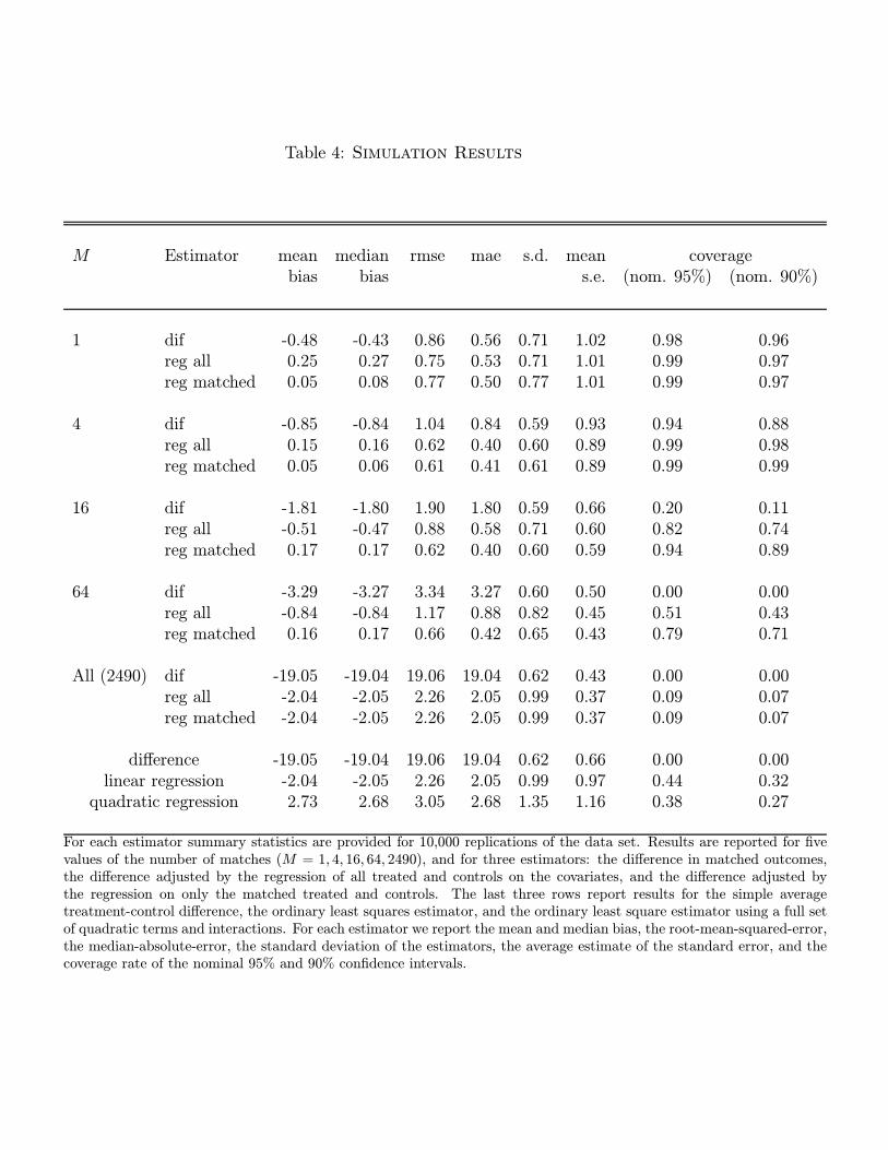
6. Simulations

In this section we discuss some simulations designed to assess the performance of the

various matching estimators in this context. To make the evaluation more credible we

simulate data sets that in a number of ways resemble the Lalonde data set analyzed in the

previous section fairly closely.

In the simulation we have nine regressors, designed to match the following variables in the

19

Lalonde data set: age, education, black, hispanic, married, earnings1974, unemployed1974,

earnings1975, unemployed1975. For each simulated data set we sample with replacement 185

observations from the empirical covariate distribution of the trainees, and 2490 observations

from the empirical covariate distribution of the PSID controls. This gives us the joint

distribution of covariates and treatment indicators. For the conditional distribution of the

outcome given covariates, we estimated a two-part model on the PSID controls, where the

probability of zero earnings is a logistic function of the covariates with a full set of quadratic

terms and interactions. Conditional on being positive, the log of earnings is a function of

the covariates with again a full set of quadratic terms and interactions. We then assume a

constant treatment effect of 2.0.

For each data set simulated in this way we report results for the same set of estimators.

For each estimator we report the mean and median bias, the root-mean-squared-error, the

median-absolute-error, the standard deviation, the average estimated standard error, and

the coverage rates for nominal 95% and 90% confidence intervals. The results are reported

in Table 4.

In terms of rmse and mae the matching estimator using regression adjustment with the

regression only using the matched observations is best with 4 or 16 matches, although the

matching estimator with regression adjustment based on all observations is close. However,

the matched regression estimator is far better in terms of bias. The simple matching estima-

tor does not perform as well neither in terms of bias or rmse. The pure regression adjustment

estimators do not perform very well. They have high rmse and substantial bias.

In terms of coverage rates the matching estimators have higher than nominal coverage

rates, which is somewhat surprising. The regression estimators have lower than nominal

coverage rates.

7. Conclusions

In this paper we derive large sample properties of simple matching estimators. We point

20

out that with more than three continuous covariates the bias will dominate the variance

in large samples. We suggest a bias-adjustment that removes the asymptotic bias. The

resulting estimator is simple to implement and appears to perform well in simulations.

21

References

Ashenfelter, O., and D. Card, (1985), “Using the Longitudinal Structure of Earnings to

Estimate the Effect of Training Programs”, Review of Economics and Statistics, 67, 648-660.

Barnow, J. Cain, and A. Goldberger

Card, D., and Sullivan, (1988), “Measuring the Effect of Subsidized Training Programs

on Movements In and Out of Employment”, Econometrica, vol. 56, no. 3 497—530.

Cochran, W., (1968) “The Effectiveness of Adjustment by Subclassification in Removing

Bias in Observational Studies”, Biometrics 24, 295-314.

Cochran, W., and D. Rubin (1973) “Controlling Bias in Observational Studies: A Review”

Sankhya, 35, 417-46.

Dehejia, R., and S. Wahba, (1999), “Causal Effects in Nonexperimental Studies: Reevalu-

ating the Evaluation of Training Programs”, Journal of the American Statistical Association,

94, 1053-1062.

Friedlander, D., and P. Robins, (1995), “Evaluating Program Evaluations: New Ev-

idence on Commonly Used Nonexperimental Methods”, American Economic Review, Vol.

85, p 923—937.

Gradshteyn, I.S. and I.M. Ryzhik, (2000), Table of Integrals, Series, and Products. 6th

ed. New York: Academic Press.

Gu, X., and P. Rosenbaum, (1993), “Comparison of Multivariate Matching Methods:

Structures, Distances and Algorithms”, Journal of Computational and Graphical Statistics,

2, 405-20.

Hahn, J., (1998), “On the Role of the Propensity Score in Efficient Semiparametric Estimation

of Average Treatment Effects,” Econometrica 66 (2), 315-331.

Heckman, J., and J. Hotz, (1989), ”Alternative Methods for Evaluating the Impact of

Training Programs”, (with discussion), Journal of the American Statistical Association.

Heckman, J., and R. Robb, (1984), “Alternative Methods for Evaluating the Impact of

Interventions,” in Heckman and Singer (eds.), Longitudinal Analysis of Labor Market Data,

22

Cambridge, Cambridge University Press.

Heckman, J., H. Ichimura, and P. Todd, (1997), “Matching as an Econometric Evalu-

ation Estimator: Evidence from Evaluating a Job Training Program,” Review of Economic

Studies 64, 605-654.

Heckman, J., H. Ichimura, and P. Todd, (1998), “Matching As An Econometric Evalu-

ations Estimator,” Review of Economic Studies 65, 261-294.

Hirano, K., G. Imbens, and G. Ridder, (2000), “Efficient Estimation of Average Treat-

ment Effects Using the Estimated Propensity Score” NBER Working Paper.

Ichimura, H., and O. Linton, (2001), “Trick or Treat: Asymptotic Expansions for some

Semiparametric Program Evaluation Estimators.” unpublished manuscript, London School

of Economics.

Lechner, M, (1998), “Earnings and Employment Effects of Continuous Off-the-job Training

in East Germany After Unification,” Journal of Business and Economic Statistics.

Ming, K., and P. Rosenbaum, (2000), “Substantial Gain in Bias Reduction from Matching

with a Variable Number of Controls”, Biometrics.

Moller, J., (1994), Lectures on Random Voronoi Tessellations, Springer Verlag, New York.

Okabe, A., B. Boots, K. Sugihara, and S. Nok Chiu, (2000), Spatial Tessellations:

Concepts and Applications of Voronoi Diagrams, 2nd Edition, Wiley, New York.

Olver, F.W.J., (1974), Asymptotics and Special Functions. Academic Press, New York.

Quade, D., (1982), “Nonparametric Analysis of Covariance by Matching”, Biometrics, 38:,

597-611.

Robins, J., and A. Rotnitzky, (1995), “Semiparametric Efficiency in Multivariate Regres-

sion Models with Missing Data,” Journal of the American Statistical Association, Vol. 90,

No. 429, 122-129.

Rosenbaum, P., (1988), “Conditional Permutation Tests and the Propensity Score in Ob-

servational Studies,” Journal of the American Statistical Association, 79, 565-74.

Rosenbaum, P., (1988), “Optimal Matching in Observational Studies”, Journal of the Amer-

23

ican Statistical Association, 84, 1024-32.

Rosenbaum, P., (1995), Observational Studies, Springer Verlag, New York.

Rosenbaum, P., (2000), “Covariance Adjustment in Randomized Experiments and Observa-

tional Studies,” forthcoming, Statistical Science.

Rosenbaum, P., and D. Rubin, (1983), “The Central Role of the Propensity Score in

Observational Studies for Causal Effects”, Biometrika, 70, 41-55.

Rosenbaum, P., and D. Rubin, (1985), “Constructing a Control Group Using Multivariate

Matched Sampling Methods that Incorporate the Propensity Score”, American Statistician,

39, 33-38.

Rotnitzky, A., and J. Robins, (1995), “Semiparametric Regression Estimation in the

Presence of Dependent Censoring,” Biometrika, Vol. 82, No. 4, 805-820.

Rubin, D., (1973a), “Matching to Remove Bias in Observational Studies”, Biometrics, 29,

185-203.

Rubin, D., (1973b), “The Use of Matched Sampling and Regression Adjustments to Remove

Bias in Observational Studies”, Biometrics, 29, 185-203.

Rubin, D., (1977), “Assignment to Treatment Group on the Basis of a Covariate,” Journal

of Educational Statistics, 2(1), 1-26.

Rubin, D. B., (1978a), ”Bayesian inference for causal effects: The Role of Randomization”,

Annals of Statistics, 6:34—58.

Rubin, D., (1979), “Using Multivariate Matched Sampling and Regression Adjustment to

Control Bias in Observational Studies”, Journal of the American Statistical Association, 74,

318-328.

Rubin, D., and N. Thomas, (1992), “Affinely Invariant Matching Methods with Ellipsoidal

Distributions,” Annals of Statistics 20 (2) 1079-1093.

Rubin, D., and N. Thomas, (1992), “Characterizing the Effect of Matching using Linear

Propensity Score Methods with Normal Distributions,” Biometrika 79, 797-809.

Rubin, D., and N. Thomas, (1996), “Matching Using Estimated Propensity Scores: Relat-

24

ing Theory to Practice,” Biometrics 52, 249-264.

Shadish, W., T. Cook and D. Campbell, (2001), Experimental and Quasi-Experimental

Designs, Houghton Mifflin, Boston, MA.

Stoyan, D., W. Kendall, and J. Mecke, (1995), Stochastic Geometry and its Applica-

tions, 2nd Edition, Wiley, New York.

Stroock, D.W., (1994), A Concise Introduction to the Theory of Integration. Birkhauser,

Boston.

Yatchew, A., (1999), “Differencing Methods in Nonparametric Regression: Simple Tech-

niques for the Applied Econometrician”, Working Paper, Department of Economics, Univer-

sity of Toronto.

25

Appendix

Assumption 1 (Random Sampling)

Yi,Xi,Wi)Ni=1 are independent and identically distributed.

Assumption 2 (Covariate Support)

The support of X is X ⊂ r, the Cartesian product of compact intervals, with absolutely

continous density fX(x) that is bounded and bounded away from zero on X .

Assumption 3 (Finite Moments)

The first two moments of Yw and Y (0) given X = x are finite for all x ∈ X .

Assumption 4 (Propensity Score)

The propensity score e(x) = Pr(T = 1|X = x) is bounded away from zero and one.

Assumption 5 (Unconfoundedness)

W ⊥ Y (1), Y (0) X.

Assumption 6 (Rates of Power Series)

K4/N → 0.

Assumption 7 (Derivatives of Expectations) There is a C such that for each multi-

index λ the λth partial derivative of µw(x) exist for w = c, t and are bounded by C|λ|.

First we state some additional lemmas.

Theorem 3 (Uniform Convergence of Series Estimators of Derivatives of

Regression Functions, Newey 1993)

Suppose Assumptions ?-? hold. Then for any alpha > 0 and non-negative integer d,

|µw(·)− µw(·)|d = Op K1+2r (K/N)1/2 +K−α ,

for w = c, t.

26

Proof: Assumptions 3.1, 4.1, 4.2 and 4.3 in Newey (1993) are satisfied, implying that

Newey’s Theorem 4.4 applies.

Lemma 6 (Distribution of Matching Discrepancy)

Suppose Assumptions ??-?? hold. Then

Dm(Xi) = Op(N−1/r)

Lemma 7 (Infeasible versus Feasible Bias Correction)

Suppose Assumptions ??-?? hold. Then

µw(Xi)− µw(Xjm(i))− µw(Xi)− µw(Xjm(i)) = op(N−1/2),

for w = c, t.

Proof

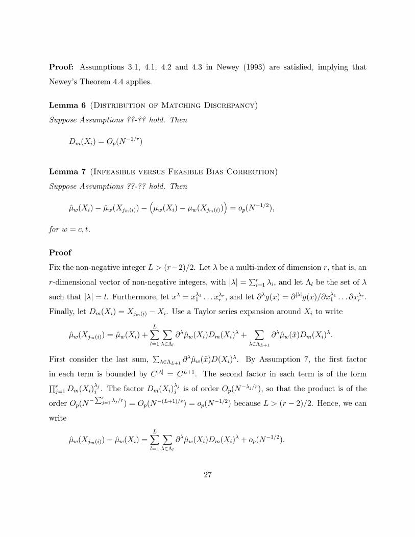
Fix the non-negative integer L > (r−2)/2. Let λ be a multi-index of dimension r, that is, anr-dimensional vector of non-negative integers, with |λ| = r

i=1 λi, and let Λl be the set of λ

such that |λ| = l. Furthermore, let xλ = xλ11 . . . xλrr , and let ∂λg(x) = ∂|λ|g(x)/∂xλ11 . . . ∂xλrr .

Finally, let Dm(Xi) = Xjm(i) −Xi. Use a Taylor series expansion around Xi to write

µw(Xjm(i)) = µw(Xi) +L

l=1 λ∈Λl∂λµw(Xi)Dm(Xi)

λ +λ∈ΛL+1

∂λµw(x)Dm(Xi)λ.

First consider the last sum, λ∈ΛL+1 ∂λµw(x)D(Xi)

λ. By Assumption 7, the first factor

in each term is bounded by C |λ| = CL+1. The second factor in each term is of the form

rj=1Dm(Xi)

λjj . The factor Dm(Xi)

λjj is of order Op(N

−λj/r), so that the product is of the

order Op(N− r

j=1λj/r) = Op(N

−(L+1)/r) = op(N−1/2) because L > (r − 2)/2. Hence, we canwrite

µw(Xjm(i))− µw(Xi) =L

l=1 λ∈Λl∂λµw(Xi)Dm(Xi)

λ + op(N−1/2).

27

Using the same argument as we used for the estimated regression function µw(x) we have

for the true regression function µw(x),

µw(Xjm(i))− µw(Xi) =L

l=1 λ∈Λl∂λµw(Xi)Dm(Xi)

λ + op(N−1/2).

Now consider the difference between these two expressions:

µw(Xjm(i))− µw(Xi)− µw(Xjm(i))− µw(Xi)

=L

l=1 λ∈Λl∂λµw(Xi)− ∂λµw(Xi) ·Dm(Xi)λ + op(N−1/2).

Consider for a particular λ ∈ Λl the term ∂λµw(Xi)− ∂λµw(Xi) · Dm(Xi)λ. The secondfactor is, using the same argument as before, of order Op(N

−l/r). Since l ≥ 1, the secondfactor is at most Op(N

−1/r). Now consider the first factor. By Theorem 3, this is of order

Op K1+2r (K/N)1/2 +K−α . With K = N δ, this is Op N

δ(3/2+2r)−1/2 +N−αδ(1+2r) . We

can choose α large enough so that for any given δ the first term dominates. Hence the order of

the product is Op Nδ(3/2+2r)−1/2 ·Op(N−1/r) Given that by Assumption ?? δ < 2/(3r+4r2)

we have δ(3/2 + 2r)− 1/2 < 1/r − 1/2, and therefore the order is op(N−1/2). 2Proof of Theorem 2

The difference τ−bcm − τ bcm can be written as

τ−bcm − τ bcm =1

N

i|wi=c

µ(Xi, 1)− µ(1)(Xjm(i))− µ(Xi, 1)− µ(1)(Xjm(i))

+i|wi=t

µ(Xi, 0)− µ(0)(Xjm(i))− µ(Xi, 0)− µ(0)(Xjm(i)) .

Each of these terms are of order op(N−1/2). There are N of them, with a factor 1/N . Hence

the sum is of order op(N−1/2).

Proof of Lemma 1

Pr(km,N = 1|X1 = x)

28

=N − 1m− 1 (Pr( X − z > x− z ))N−m (Pr( X − z ≤ x− z ))m−1

=N − 1m− 1 (1− Pr( X − z < x− z ))N−m (Pr( X − z ≤ x− z ))m−1 .

Hence,

fDm,N (v) = NN − 1m− 1 f(z + v) (1− Pr( X − z ≤ x− z ))N−m

× (Pr( X − z ≤ x− z ))m−1 .

Therefore,

EDm,N = NN − 1m− 1 Im,N ,

where

Im,N =kv f(z + v) (1− Pr( X − z ≤ x− z ))N−m (Pr( X − z ≤ x− z ))m−1 dv.

Change variables to polar coordinates to get:

Im,N =∞

0rk−1

Skrω f(z + rω)λSk(dω) (1− Pr( X − z ≤ r))N−m (Pr( X − z ≤ r))m−1 dr

=∞

0rk−1

Skrω f(z + rω)λSk(dω) 1−

r

0sk−1

Skf(z + sω)λSk(dω) ds

N−m

×r

0sk−1

Skf(z + sω)λSk(dω) ds

m−1dr

=∞

0e−Np(r) a(r) dr,

where

p(r) = − log 1−r

0sk−1

Skf(z + sω)λSk(dω) ds ,

29

and

a(r) = rk ·Skω f(z + rω)λSk(dω)

r

0sk−1

Skf(z + sω)λSk(dω) ds

m−1

1−r

0sk−1

Sk

f(z + sω)λSk(dω) dsm .

That is, a(r) = q(r)b(r), q(r) = rkc(r), and b(r) = (g(r))m−1, where

c(r) = Skω f(z + rω)λSk(dω)

1−r

0sk−1

Skf(z + sω)λSk(dω) ds

,

g(r) =

r

0sk−1

Skf(z + sω)λSk(dω) ds

1−r

0sk−1

Skf(z + sω)λSk(dω) ds

.

Note that

dg

dr(r) = rk−1 Sk

f(z + rω)λSk(dω)ds

1−r

0sk−1

Skf(z + sω)λSk(dω) ds

2 .

Therefore, the first non-zero derivative of g at zero is

dkg

drk(0) = (k − 1)!f(z)

SkλSk(dω).

Using standard results on higher order derivatives of composite functions (see, e.g., Grad-

shteyn and Ryzhik 2000), it can be seen that the first non-zero derivative of b at zero is:

d(m−1)kbdr(m−1)k

(0) =((m− 1)k)!(k!)m−1

· dkg

drk(z)

m−1

=((m− 1)k)!km−1

· f(z)SkλSk(dω)

m−1.

It has been shown above that the first non-zero derivative of q(r) at zero is

dk+1q

drk+1(0) = (k + 1)!

Skωω λSk(dω)

df

dx(z)

30

= (k + 1)! Sk

λSk(dω)

k

df

dx(z).

Therefore, the first non-zero derivative of a(r) at zero is

dmk+1a

drmk+1(0) =

mk + 1k + 1

d(m−1)kbdr(m−1)k

(0)dk+1q

drk+1(0) =

(mk + 1)!

kmf(z)

SkλSk(dω)

m 1

f(z)

df

dx(z).

So, in a neigborhood of zero we have that

a(r) =∞

t=0

a(1)rmk+1+t, with a(1) =1

(mk + 1 + t)!

dmk+1+ta

drmk+1+t(0).

It has been shown above that p(0) = 0 and the first non-zero derivative of p(r) at zero is

dkp

drk(0) = (k − 1)!f(z)

Sk

λSk(dω).

In a neigborhood of zero we have that:

p(r) =∞

t=0

p(1)rk+t, with p(1) =1

(k + t)!

dk+tp

drk+t(0).

Applying Theorem 8.1 in Olver (1974), we get

Im,N = Γmk + 2

k

a0

kp(mk+2)/k0

1

N (mk+2)/k+ o

1

N (mk+2)/k

= Γmk + 2

k

1

k

f(z)

k SkλSk(dω)

−2/k1

f(z)

df

dx(z)

1

N (mk+2)/k+ o

1

N (mk+2)/k.

Now, since

Nm/(m− 1)!N

N − 1m− 1

− 1 = o(1),

we have that

EDm,N = Γmk + 2

k

1

(m− 1)!k

f(z) πk/2

Γ 1 + k2

−2/k 1

f(z)

df

dx(z)

1

N2/k+ o

1

N2/k.

31

To get the result for EDm,NDm,N , notice that

EDm,NDm,N = NN − 1m− 1 Im,N ,

where

Im,N =kvv f(z + v) (1− Pr( X − z ≤ x− z ))N−m (Pr( X − z ≤ x− z ))m−1 dv

=∞

0rk−1

Skr2ωω f(z + rω)λSk(dω) 1−

r

0sk−1

Skf(z + sω)λSk(dω) ds

N−m

×r

0sk−1

Skf(z + sω)λSk(dω) ds

m−1dr

=∞

0e−Np(r) a(r) dr,

p(r) = − log 1−r

0sk−1

Skf(z + sω)λSk(dω) ds ,

and

a(r) = rk+1 ·Skωω f(z + rω)λSk(dω)

r

0sk−1

Skf(z + sω)λSk(dω) ds

m−1

1−r

0sk−1

Skf(z + sω)λSk(dω) ds

m .

That is, a(r) = q(r)b(r), q(r) = rk+1c(r), and b(r) = (g(r))m−1, where

c(r) = Sk

ωω f(z + rω)λSk(dω)

1−r

0sk−1

Sk

f(z + sω)λSk(dω) ds,

g(r) =

r

0sk−1

Skf(z + sω)λSk(dω) ds

1−r

0sk−1

Skf(z + sω)λSk(dω) ds

.

As shown above, q(0) = 0 and the first non-zero derivative of q(r) at zero is

dk+1q

drk+1(0) = (k + 1)!f(z)

Skωω λSk(dω) = (k + 1)!f(z)

Sk

λSk(dω)

k· I,

32

and

d(m−1)kbdr(m−1)k

(0) =((m− 1)k)!km−1

· f(z)SkλSk(dω)

m−1.

Therefore, the first non-zero derivative of a(r) at zero is

dmk+1a

drmk+1(0) =

mk + 1k + 1

d(m−1)kbdr(m−1)k

(0)dk+1q

drk+1(0)

= (mk + 1)! f(z) SkλSk(dω)

k

m

· I.

So, in a neigborhood of zero we have that

a(r) =∞

t=0

a(1)rmk+1+t, with a(1) =1

(mk + 1 + t)!

dmk+1+ta

drmk+1+t(0).

It has been shown above that p(0) = 0 and the first non-zero derivative of p(r) at zero is

dkp

drk(0) = (k − 1)!f(z)

SkλSk(dω).

In a neigborhood of zero we have that:

p(r) =∞

t=0

p(1)rk+t, with p(1) =1

(k + t)!

dk+tp

drk+t(0).

Applying Theorem 8.1 in Olver (1974), we get

Im,N = Γmk + 2

k

a0

kp(mk+2)/k0

1

N (mk+2)/k+ o

1

N (mk+2)/k

= Γmk + 2

k

1

k

f(z)

k SkλSk(dω)

−2/k1

N (mk+2)/k· I + o 1

N (mk+2)/k.

Now, since

Nm/(m− 1)!N

N − 1m− 1

− 1 = o(1),

we have that

EDm,NDm,N = Γmk + 2

k

1

(m− 1)!k

f(z) πk/2

Γ 1 + k2

−2/k 1

N2/k· I + o 1

N2/k.

33

Using the same techniques as for the first two moments, E Dm,N3 = N · Im,N , where

Im,N =∞

0e−Np(r) a(r) dr,

p(r) = − log 1−r

0sk−1

Skf(z + sω)λSk(dω) ds ,

and

a(r) = rk+2 ·Skf(z + rω)λSk(dω)

r

0sk−1

Skf(z + sω)λSk(dω) ds

m−1

1−r

0sk−1

Skf(z + sω)λSk(dω) ds

m .

That is, a(r) = q(r)b(r), q(r) = rk+2c(r), and b(r) = (g(r))m−1, where

c(r) = Skf(z + rω)λSk(dω)

1−r

0sk−1

Skf(z + sω)λSk(dω) ds

,

g(r) =

r

0sk−1

Skf(z + sω)λSk(dω) ds

1−r

0sk−1

Skf(z + sω)λSk(dω) ds

.

All the derivatives of q at zero of order smaller than k+2 are equal to zero. In addition,

all the derivatives of b at zero of order smaller than (m − 1)k are equal to zero. Therefore,all the derivatives of a at zero of order smaller than mk + 2 are equal to zero. Applying the

results in Olver (1974), we obtain

Im,N = O1

N (mk+3)/k.

Therefore

E Dm,N3 = O

1

N3/k= o

1

N2/k.

2

34

Proof of Lemma 4 Order the observations so that the first N1 observations have ti = 1

and the last N0 observations have ti = 0. Then partition the matrix A as

A =IN1 −A01/M

A10/M −IN0 ,

with IN1 and IN0 identity matrices of rank N1 and N0 respectively. Note that A01 and A10

are N0 × N1 and N1 × N0 dimensional matrices with all elements equal to zero or one. Inaddition, A01ιN1 is a N0 dimensional vector with all elements equal to M , and A10ιN0 is

a N1 dimensional vector with all elements equal to M . The vector A01ιN1 has ith element

equal to KM(i), and A10ιN0 has ith element equal to KM(i+N1). Therefore,

ιN1A01A01ιN1 = (A01ιN1) (A01ιN1) =i∈I1

KM(i)2,

because the typical elemenent of A01ιN1 is equal to KM(i). Similarly

ιN1A01A01ιN1 =i∈I0

KM(i)2.

After these preliminaries consider the matrix AA :

AA =IN1 +A01A01/M

2 (A10 +A01)/M(A10 +A01)/M IN0 +A10A10/M

2 .

Hence

ιNAA ιN = ιN1(IN1 +A01A01/M2)ιN1 + 2ιN1(A10/M +A01/M)ιN0

+ιN0(IN0 +A10A10/M2)ιN0

= N1 + ιN1A01A01ιN1/M2 + 2(N1M +N0M) +N0 + ιN0A10A10ιN0/M

2

= 3N +1

M2

N

i=1

KM(i)2.

2

35

Lemma 8 The exact conditional distribution of Km(i) is,

KM(i) T1, . . . , TN , Xjj∈I1 , Ti = 1 ∼ Binomial N0,AM (i)

f0(z)dz ,

and

KM(i) T1, . . . , TN , Xjj∈I0 , Ti = 0 ∼ Binomial N1,AM (i)

f1(z)dz .

Let us consider in more detail, for the special case considered in this section with a scalar

covariate, the set AM(i). First, let rt(x) be the number of units with Ti = t and Xi ≥ x.Then, define X(i,k) = Xj if rTi(Xi)− rTi(Xj) = k, and rTi(Xi)− limx↑Xj rTi(x) = k − 1.

Lemma 9 The set AM(i) is equal to the interval

AM(i) = (Xi/2 +X(i,−M)/2, Xi/2 +X(i,M))/2),

with width (X(i,M) −X(i,−M))/2.

Lemma 10 Given Xi = x, and Ti = 1

2N1 · f1(x)f0(x)

·AM (i)

f0(z)dzd→ Gamma (2M, 1),

and given Xi = x and Ti = 0,

2N0 · f0(x)f1(x)

·AM (i)

f1(z)dzd→ Gamma (2M, 1),

Proof: We only prove the first part of the lemma. The second part follows exactly the same

proof. First we establish that

2N1f1(x) ·AM (i)

dz = N1f1(x) X(i,M) −X(i,−M) d→ Gamma (2M, 1).

Let F1(x) be the distribution function ofX given T = 1. Then Y = F1(X(i,+M))−F1(X(i,−M))is the difference in order statistics of the uniform distribution, 2M orders apart. Hence the

36

exact distribution of Y is Beta with parameters 2M and N1. For large N1, the distribution

of N1 · Y is then Gamma with parameters 2M and 1. Now approximate N1Y as

N1Y = N1 · F1(X(i,M))− F1(X(i,−M)) ≈ N1f1(x) · X(i,M) −X(i,−M) ,

which demonstrates the first claim.

Second, we show that

2N1f1(x)

f0(x)·AM (i)

f0(z)dz − 2N1f1(x) ·AM (i)

dz = op(1).

This difference can be written as

2N1f1(x)

f0(x)·AM (i)

f0(z)dz − 2N1f1(x)f0(x)

·AM (i)

f0(x)dz = 2N1f1(x)

f0(x)·

AM (i)(f0(z)− f0(x))dz .

Because

f0(z)− f0(x) = f0(z) (z − x),

we have

||f0(z)− f0(x)|| ≤ supz||f0(z)|| · ||z − x||,

and hence we can bound the difference by

= 2N1f1(x)

f0(x)·AM (i)

dz · supz||f0(z)|| ·maxi sup

z,x∈AM (i)||z − x||.

By the first part of the proof

2N1f1(x)

f0(x)·AM (i)

dz = Op(1).

By Assumption ?? supz ||f0(z)|| is bounded, and by Lemma ?? maxi supz,x∈AM (i) ||z − x|| isop(1). Hence the product is op(1). 2

Lemma 11 The number of matches KM(i) is Z + op(1), where

E[Z2] =M2 · (1− p)2

p

f0(x)2

f1(x)dx+M2 · p2

(1− p)f1(x)

2

f0(x)dx

+M +M · (1− p)2

2p

f0(x)2

f1(x)dx+M · p2

2(1− p)f1(x)

2

f0(x)dx+ o(1).

37

Proof: Condition on Ti = 1 and Xi = x. By Lemma 10, we can write

2N1 · f1(x)f0(x)

·AM (i)

f0(z)dz = W + op(1),

where

W ∼ Gamma (2M, 1).

Let Z be a random variable with conditional distribution of Z given W equal to a binomial

distribution with parameters N0 and Wf0(x)/(F1(x)N1). Then, because the distribution of

Km(i) given 2N1 · f1(x)f0(x)· AM (i)

f0(z)dz is the same as the distribution of Z given W , and

because the distribution of 2N1 · f1(x)f0(x)· AM (i) f0(z)dz converges to that of W , the distribution

of KM(i) converges to that of Z. This demonstrates the first part of the claim.

For the second part we calculate the second moment of Z, initially conditional on W ,

Tjj=1,...,N , and Xi = x. Suppose Ti = 1. Then

E[Z2|W,Ti = 1, Xi = x] = N20f

20 (x)

4N21f

21 (x)

W 2 +N0f0(x)

2N1f1(x)W − N0f0(x)

2

4N1f1(x)2W 2.

The latter term is of lower order and will be ignored. Then taking the expectation over W ,

(with E[W ] = 2M and E[W 2] = 4M2 + 2M), still conditioning on Ti = 1 and Xi = x gives

E[Z2|Ti = 1, Xi = x] =M2 · (1− p)2f0(x)

2

p2f1(x)2+M · (1− p)f0(x)

pf1(x)+M · (1− p)

2f0(x)2

2p2f1(x)2.

Similarly,

E[Z2|Ti = 0, Xi = x] =M2 · p2f1(x)2

(1− p)2f0(x)2 +M · pf1(x)

(1− p)f0(x) +M · p2f1(x)2

2(1− p)2f0(x)2 .

Then taking the expectation over T and X gives the desired result. 2

Proof of Lemma 5:

For a calculation of the efficiency bound in the general case see Hahn (1998). To show the

result in the lemma, we will demonstrate that

3 +1

M2E[K2

M ] = E1

e(X)+

1

1− e(X) .

38

First, write

e(x) =pf1(x)

pf1(x) + (1− p)f0(x) ,

so that

E1

e(x)=

x

pf1(x) + (1− p)f0(x)pf1(x)

(pf1(x) + (1− p)f0(x)) dx

= 1 +x

(1− p)f0(x)pf1(x)

(pf1(x) + (1− p)f0(x)) dx

= 1 + (1− p) +x

(1− p)f0(x)pf1(x)

(1− p)f0(x)dx

= 1 + (1− p) + (1− p)2

p x

f 20 (x)

f1(x)dx.

Using the same argument for E[1/(1− e(X))], and combining the results, we get

Veff/σ2 = E

1

e(X)+

1

1− e(X) = 3 +(1− p)2p x

f 20 (x)

f1(x)dx+

p2

1− p x

f 20 (x)

f1(x).dx

Hence we can write

(1− p)2p x

f20 (x)

f1(x)dx+

p2

1− p x

f 20 (x)

f1(x).dx = (Veff − 3)/σ2.

Plugging this into the variance for the matching estimator, using the expression for the

second moment of KM , we get

σ2 3 +1

M2E[K2

M ] = Veff +σ2

M+1

M(Veff − 3σ2)/2

= Veff +1

2M(Veff − σ2)/2 = Veff · 1 + 1

2M− σ2

2M

2

39

Table 1: Summary Statistics Lalonde Data

Experimental Data PSID T-statisticTrainees (N=185) Controls (N=260) Controls (N=2490) Train/ Train/mean (s.d.) mean (s.d.) mean (s.d.) Contr PSID

Age 25.8 (7.16) 25.05 (7.06) 34.85 (10.44) [1.1] [-16.0]Education 10.4 (2.01) 10.09 (1.61) 12.12 (3.08 ) [1.4] [-11.1]Black 0.84 (0.36) 0.83 (0.38) 0.25 (0.43 ) [0.5] [21.0]Hispanic 0.06 (0.24) 0.11 (0.31) 0.03 (0.18 ) [-1.9] [1.5]Married 0.19 (0.39) 0.15 (0.36) 0.87 (0.34 ) [1.0] [-22.8]Earnings ’74 2.10 (4.89) 2.11 (5.69) 19.43 (13.41) [-0.0] [-38.6]Unempl. ’74 0.71 (0.46) 0.75 (0.43) 0.09 (0.28 ) [-1.0] [18.3]Earnings ’75 1.53 (3.22) 1.27 (3.10) 19.06 (13.60) [0.9] [-48.6]Unempl ’75 0.60 (0.49) 0.68 (0.47) 0.10 (0.30 ) [-1.8] [13.76]

Earnings ’78 6.35 (7.87) 4.55 (5.48) 21.55 (15.56) [2.7] [-23.1]Unempl. ’78 0.24 (0.43) 0.35 (0.48) 0.11 (0.32 ) [-2.65] [4.0]

The first two columns give the average and standard deviation of the 185 trainees from the experimental data set.The second pair of columns give the average and standard deviation of the 260 controls from the experimentaldata set. The third pair of columns give the averages and standard deviations of the 2490 controls from thenonexperimental PSID sample. The seventh column gives t-statistics for the difference between the averages forthe experimental trainees and controls. The last column gives the t-statistics for the differences between theaverages for the experimental trainees and the PSID controls. The last two variables, earnings ’78 and unemployed’78 are post-training. All the others are pre-training variables. Earnings data are in thousands of dollars.

Table 2: Experimental and Non-experimental Estimates of Average Treat-ment Effects for Lalonde Data

M = 1 M = 4 M = 16 M = 64 All Controlsmean (s.d.) est (s.e.) est (s.e.) est (s.e.) est (s.e.)

Panel A: Experimental Estimatesdif 1.23 (0.84) 1.99 (0.79) 1.76 (0.79) 2.20 (0.80) 1.79 (0.75)reg-all 1.22 (0.84) 1.94 (0.79) 1.57 (0.80) 1.80 (0.82) 1.72 (0.77)reg-matched 1.17 (0.84) 1.84 (0.80) 1.55 (0.80) 1.74 (0.82) 1.72 (0.77)Regression Estimatesdif 1.79 (0.67)linear 1.72 (0.65)quadratic 2.27 (0.73)

Panel B: Non-experimental Estimatesdif 2.09 (1.67) 1.62 (1.71) 0.47 (1.21) -0.11 (0.90) -15.20 (0.60)reg-all 2.56 (1.69) 2.54 (1.68) 1.80 (1.14) 2.29 (0.82) 0.84 (0.62)reg-matched 2.45 (1.68) 2.51 (1.68) 2.48 (1.15) 2.26 (0.83) 0.84 (0.62)Regression Estimatesdif -15.20 (0.66)linear 0.84 (0.86)quadratic 3.26 (0.98)

Panel A reports the results for the experimental data (experimental controls and trainees), and Panel B the results for thenonexperimental data (PSID controls with experimental trainees). In each panel the top part reports results for the matchingestimators, with the number of matches equal to 1, 4, 16, 64 and 2490 (all controls). The second part reports results for threeregression adjustment estimates, based on no covariates, all covariates entering linearly and all covariates entering with a fullyset of quadratic terms and interactions. The outcome is earnings in 1978 in thousands of dollars.

Table 3: Mean Covariate Differences in Matched Groups

Average M = 1 M = 4 M = 16 M = 64 M = 2490PSID Trainees dif (s.d.) dif (s.d.) dif (s.d.) dif (s.d.) dif (s.d.)

Age 0.06 -0.80 -0.02 (0.65) -0.06 (0.60) -0.30 (0.41) -0.57 (0.57) -0.86 (0.68)Education 0.04 -0.54 -0.10 (0.44) -0.20 (0.48) -0.25 (0.39) -0.24 (0.42) -0.58 (0.66)Black -0.09 1.21 -0.00 (0.00) 0.09 (0.32) 0.35 (0.47) 0.70 (0.66) 1.30 (0.80)Hispanic -0.01 0.14 -0.00 (0.00) 0.00 (0.00) 0.00 (0.00) 0.01 (0.03) 0.15 (1.30)Married 0.12 -1.64 0.00 (0.00) -0.06 (0.30) -0.33 (0.46) -0.90 (0.85) -1.76 (1.02)Earnings ’74 0.09 -1.18 -0.01 (0.10) -0.01 (0.12) -0.05 (0.17) -0.15 (0.30) -1.26 (0.36)Unempl ’74 -0.13 1.72 0.00 (0.00) 0.02 (0.17) 0.24 (0.40) 0.41 (0.72) 1.85 (1.36)Earnings ’75 0.09 -1.18 -0.04 (0.17) -0.07 (0.15) -0.11 (0.19) -0.19 (0.26) -1.26 (0.23)Unempl ’75 -0.10 1.36 0.00 (0.00) 0.00 (0.05) 0.03 (0.28) 0.10 (0.41) 1.46 (1.44)

Log OddsProp Score -7.08 1.08 0.21 (0.99) 0.56 (1.13) 1.70 (1.14) 3.20 (1.49) 8.16 (2.13)

In this table all covariates have been normalized to have mean zero and unit variance. The first two columns present theaverages for the experimental trainees and the PSID controls. The remaining pairs of columns present the average differencewithin the matched pairs and the standard deviation of this difference for matching based on 1, 4, 16, 64 and 2490 matches.For the last variable the the logarithm of the odds ratio of the propensity score is used. This log odds ratio has mean -6.52and standard deviation 3.30 in the sample.

Table 4: Simulation Results

M Estimator mean median rmse mae s.d. mean coveragebias bias s.e. (nom. 95%) (nom. 90%)

1 dif -0.48 -0.43 0.86 0.56 0.71 1.02 0.98 0.96reg all 0.25 0.27 0.75 0.53 0.71 1.01 0.99 0.97reg matched 0.05 0.08 0.77 0.50 0.77 1.01 0.99 0.97

4 dif -0.85 -0.84 1.04 0.84 0.59 0.93 0.94 0.88reg all 0.15 0.16 0.62 0.40 0.60 0.89 0.99 0.98reg matched 0.05 0.06 0.61 0.41 0.61 0.89 0.99 0.99

16 dif -1.81 -1.80 1.90 1.80 0.59 0.66 0.20 0.11reg all -0.51 -0.47 0.88 0.58 0.71 0.60 0.82 0.74reg matched 0.17 0.17 0.62 0.40 0.60 0.59 0.94 0.89

64 dif -3.29 -3.27 3.34 3.27 0.60 0.50 0.00 0.00reg all -0.84 -0.84 1.17 0.88 0.82 0.45 0.51 0.43reg matched 0.16 0.17 0.66 0.42 0.65 0.43 0.79 0.71

All (2490) dif -19.05 -19.04 19.06 19.04 0.62 0.43 0.00 0.00reg all -2.04 -2.05 2.26 2.05 0.99 0.37 0.09 0.07reg matched -2.04 -2.05 2.26 2.05 0.99 0.37 0.09 0.07

difference -19.05 -19.04 19.06 19.04 0.62 0.66 0.00 0.00linear regression -2.04 -2.05 2.26 2.05 0.99 0.97 0.44 0.32

quadratic regression 2.73 2.68 3.05 2.68 1.35 1.16 0.38 0.27

For each estimator summary statistics are provided for 10,000 replications of the data set. Results are reported for fivevalues of the number of matches (M = 1, 4, 16, 64, 2490), and for three estimators: the difference in matched outcomes,the difference adjusted by the regression of all treated and controls on the covariates, and the difference adjusted bythe regression on only the matched treated and controls. The last three rows report results for the simple averagetreatment-control difference, the ordinary least squares estimator, and the ordinary least square estimator using a full setof quadratic terms and interactions. For each estimator we report the mean and median bias, the root-mean-squared-error,the median-absolute-error, the standard deviation of the estimators, the average estimate of the standard error, and thecoverage rate of the nominal 95% and 90% confidence intervals.