Simple and Trustworthy Cluster-Robust GMM Inference

Jungbin Hwang∗

Department of Economics,

University of Connecticut†

September 9, 2016

Abstract

This paper develops a new asymptotic theory for two-step GMM estimation and inference

in the presence of clustered dependence. While conventional asymptotic theory completely

ignores the variability in the cluster-robust GMM weighting matrix, the new asymptotic theory

takes it into account, leading to more accurate approximations. The key difference between

these two types of asymptotics is whether the number of clusters G is regarded as small

(fixed) or growing when the sample size increases. Under the new small-G asymptotics, the

centered two-step GMM estimator and the two continuously-updating estimators have the

same asymptotic mixed normal distribution. In addition, the J-statistic, the trinity of two-

step GMM statistics (QLR, LM and Wald), and the t-statistic are all asymptotically pivotal,

and each can be modified to have an asymptotic standard F distribution or t distribution.

We suggest a finite sample variance correction to further improve the accuracy of the F and

t approximations. Our proposed asymptotic F and t tests are very appealing to practitioners

because our test statistics are simple modifications of the usual test statistics, and the F and

t critical values are readily available from standard statistical tables. A Monte Carlo study

shows that our proposed tests are much more accurate than existing tests. We also apply our

methods to an empirical study on the causal effect of access to domestic and international

markets on household consumption in rural China. The results suggest that the effect of access

to markets may be lower than the previous finding.

∗Email: jungbin.hwang@uconn.edu. Correspondence to: Department of Economics365 Fairfield Way, U-1063Storrs, CT 06269-1063.†I am indebt to Yixiao Sun, Graham Elliott, Andres Santos, and Minseong Kim that helped greatly improve

this paper. I would also like to thank Eli Berman, Stephane Bonhomme, Kenneth Couch, Gordon Dahl, James D.Hamilton, Ivan Jeliazkov, Harim Kim, Michal Kolesár, Stepehn L. Ross, and other seminar partcipants at UCSD,UCONN, UCI, and 2016 North Ameriacan Meeting of Econometric Society.

1

1 Introduction

Clustering is a common feature for many cross-sectional and panel data sets in applied economics.

The data often come from a number of independent clusters with a general dependence structure

within each cluster. For example, in development economics, data are often clustered by geographi-

cal regions, such as village, county and province (e.g., de Brauw and Giles 2008; Pepper 2002; Dube

et al. 2010). In empirical finance and industrial organization, firm level data are often clustered

at the industry level (Samila and Sorenson, 2011; Bharath et al., 2013), and in many educational

studies, students’test scores are clustered at the classroom or school level (Andrabi et.al, 2011).

Because of learning from daily interactions, the presence of common shocks, and for many other

reasons, individuals in the same cluster will be interdependent while those from different clusters

tend to be independent. Failure to control for within group or cluster correlation often leads to

downwardly biased standard errors and spurious statistical significance.

Seeking to robustify inference, many practical methods employ clustered covariance estimators

(CCE). See White (1984), Liang and Zeger (1986), Arellano (1987) for seminal methodological con-

tributions, and Wooldridge (2003) and Cameron and Miller (2015) for overviews of the CCE and

its applications. It is now well known that standard test statistics based on the CCE are either

asymptotically chi-squared or normal. The chi-squared and normal approximations are obtained

under the so-called large-G asymptotic specification, which requires the number of clusters G to

grow with the sample size. The key ingredient behind these approximations is that the CCE be-

comes concentrated at the true asymptotic variance as G diverges to infinity. In effect, this type

of asymptotics ignores the estimation uncertainty in the CCE despite its high variation in finite

samples, especially when the number of clusters is small. In practice, it is not unusual to have

a data set that has a small number of clusters. For example, if clustering is based on large geo-

graphical regions such as U.S. states and regional blocks of neighboring countries, (e.g., Bertrand

et al., 2004; Obstfeld et al., 2010; Ibragimov and Müller, 2015), we cannot convincingly claim that

the number of cluster is large so that the large-G asymptotic approximations are applicable. In

fact, there is ample simulation evidence that the large-G approximation can be very poor when the

number of clusters is not large (e.g., Donald and Lang, 2007; Cameron et al., 2008; Bester et al.,

2011; Mackinnon and Webb, 2014).

In this paper, we adopt an alternative approach that yields more accurate approximations, and

that works well whether or not the number of clusters is large. In fact, our approximations work

especially well when the chi-squared and normal approximations are poor. They are obtained from a

limiting thought experiment where the number of clusters G is held fixed. Under this small (fixed)-

G asymptotics, the CCE no longer asymptotically degenerates; instead, it converges in distribution

to a random matrix that is proportional to the true asymptotic variance. The random limit of the

CCE has profound implications for the analyses of the asymptotic properties of GMM estimators

and the corresponding test statistics.

We start with the first-step GMM estimator where the underlying model is possibly over-

2

identified and show that suitably modified Wald and t-statistics converge weakly to standard F

and t distributions, respectively. The modification is easy to implement because it involves only

a known multiplicative factor. Similar results have been obtained by Hansen (2007) and Bester,

Conley and Hansen (2011), which employ a CCE type HAC estimator but consider only linear

regressions and M-estimators for an exactly identified model.

We then consider the two-step GMM estimator that uses the CCE as a weighting matrix. Be-

cause the weighting matrix is random even in the limit, the two-step estimator is not asymptotically

normal. The form of the limiting distribution depends on how the CCE is constructed. If the CCE

is based on the uncentered moment process, we obtain the so-called uncentered two-step GMM

estimator. We show that the asymptotic distribution of this two-step GMM estimator is highly

nonstandard. As a result, the associated Wald statistic is not asymptotically pivotal. However,

it is surprising that the J-statistic is still asymptotically pivotal. Furthermore, we show that the

limiting distribution of the J-statistic can be represented as an increasing function of a standard

F random variable. So critical values are readily available from standard statistical tables and

software packages.

Next, we establish the asymptotic properties of the “centered”two-step GMM estimator1 whose

weighting matrix is constructed using recentered moment conditions. Invoking centering is not

innocuous for an over-identified GMM model because the empirical moment conditions, in this

case, are not equal to zero in general. Under the traditional large-G asymptotics, recentering

does not matter in large samples because the empirical moment conditions are asymptotically zero

and here are ignorable, even though they are not identically zero in finite sample. In contrast,

under the small-G asymptotics, recentering plays two important roles: it removes the first order

effect of the estimation error in the first-step estimator, and it ensures that the weighting matrix

is asymptotically independent of the empirical moment conditions. With the recentered CCE as

the weighting matrix, the two-step GMM estimator is asymptotically mixed normal. The mixed

normality reflects the high variation of the feasible two-step GMM estimator as compared to the

infeasible two-step GMM estimator, which is obtained under the assumption that the ‘effi cient’

weighing matrix is known. The mixed-normality allows us to construct the Wald and t-statistics

that are asymptotically nuisance parameter free.

We also consider two types of continuous updating (CU) estimators. The first type continuously

updates the first order conditions (FOC) underlying the two-step GMM estimator. Given that

FOC’s can be regarded as the empirical version of generalized estimating equations (GEE), we call

this type of CU estimator the CU-GEE estimator. The second type continuously updates the GMM

criterion function, leading to the CU-GMM estimator, which was first suggested by Hansen, Heaton

and Yaron (1996). Both CU estimators are designed to improve the finite sample performance of

two-step GMM estimators. Interestingly, we show that the continuous updating scheme has a

built-in recentering feature. So in terms of the first order asymptotics, it does not matter whether

1Our definition of the centered two-step GMM estimator is originated from the recentered (or demeaned) GMMweighting matrix, and it should not be confused with “centering”the estimator itself.

3

the empirical moment conditions are recentered or not. We find that the centered two-step GMM

estimator and the two CU estimators are all first-order asymptotically equivalent under the small-

G asymptotics. This result provides a theoretical justification for using the recentered CCE in a

two-step GMM framework.

To relate the small-G asymptotic pivotal distributions to standard distributions, we introduce

simple modifications to the Wald and t statistics associated with the centered two-step GMM

and CU estimators. We show that the modified Wald and t statistics are asymptotically F and t

distributed, respectively. This result resembles the corresponding result that is based on the first-

step GMM estimator. It is important to point out that the proposed modifications are indispensable

for our asymptotic F and t theory. In the absence of the modifications, the Wald and t statistics

converge in distribution to nonstandard distributions, and as a result, critical values have to be

simulated. The modifications involve only the standard J-statistic, and it is very easy to implement

because the modified test statistics are scaled versions of the original Wald test statistics with the

scaling factor depending on the J-statistic. Significantly, the combination of the Wald statistic and

the J-statistic enables us to develop the F approximation theory.

Finally, although recentering removes the first order effect of the first-step estimation error, the

centered two-step GMM estimator still faces some extra estimation uncertainty in the first-step

estimator. The main source of the problem is that we have to estimate the unobserved moment

process based on the first-step estimator. To capture the higher order effect, we propose to retain

one more term in our stochastic approximation that is asymptotically negligible. The expansion

helps us develop a finite sample correction to the asymptotic variance estimator. Our correction

resembles that of Windmeijer (2005), which considers variance correction for a two-step GMM

estimator but only in the i.i.d. setting. We show that the finite sample variance correction does not

change the limiting distributions of the test statistics, but they can help improve the finite sample

performance of our tests.

Monte Carlo simulations show that our new tests have a much more accurate size than existing

tests via standard normal and chi-square critical values, especially when the number of clusters G

is not large. An advantage of our procedure is that the test statistics do not entail much extra

computational cost because the main ingredient for the modification is the usual J-statistic. There

is also no need to simulate critical values because the F and t critical values can be readily obtained

from standard statistical tables.

Our small-G asymptotics is related to fixed-smoothing asymptotics for a long run variance (LRV)

estimation in a time series setting. The latter was initiated and developed in econometric literature

by Kiefer, Vogelsang and Bunzel (2002), Kiefer and Vogelsang (2005), Müller (2007), Sun, Phillips

and Jin (2008) and Sun (2013, 2014), among others. Our new asymptotics is in the same spirit in

that both lines of research attempt to capture the estimation uncertainty in covariance estimation.

With regards to orthonormal series LRV estimation, a recent paper by Hwang and Sun (2015b)

modifies the two-step GMM statistics using the J-statistic, and shows that the modified statistics

4

are asymptotically F and t distributed. The F and t limit theory presented in this paper is similar,

but our cluster-robust limiting distributions differ from those of our predecessors in terms of the

multiplicative adjustment and the degrees of freedom. Moreover, we propose a finite sample variance

correction to capture the uncertainty embodied in the estimated moment process adequately. To

our knowledge, the finite sample variance correction provided in this paper has not been considered

in the literature on the fixed-smoothing asymptotics.

There is also a growing literature that uses the small-G asymptotics to design more accurate

cluster-robust inference. For instance, Ibragimov and Müller (2010, 2016) recently proposes a sub-

sample based t-test for a scalar parameter that is robust to heterogeneous clusters. Hansen (2007),

Stock and Watson (2008), and Bester, Conley and Hansen (2011) propose a cluster-robust F or t

tests under cluster-size homogeneity. Bell and McCaffrey (2002) and Imbens and Kolesár (2012) sug-

gest an adjusted t-critical value employing data-determined degrees of freedom. Recently, Canay,

Romano and Shaikh (2014) establishes a theory of randomization tests and suggests an alterna-

tive cluster-robust test. For other approaches, see Carter, Schnepel and Steigerwald (2013) which

proposes a measure of the effective number of clusters under the large-G asymptotics.; Cameron,

Gelbach and Miller (2008), MacKinnon and Webb (2016), and Webb (2014) which provide cluster

bootstrap approaches with asymptotic refinement. All these studies, however, mainly focus on a

simple location model or linear regressions that are special cases of exactly identified models.

The remainder of the paper is organized as follows. Section 2 presents the basic setting and

establishes the approximation results for the first-step GMM estimator under the small-G asymp-

totics. Sections 3 and 4 establish the small-G asymptotics for two-step GMM estimators and the

CU estimators, respectively. Section 5 is devoted to developing asymptotic F and t tests based on

the centered two-step GMM estimator and the CU estimators. Section 6 proposes a finite sample

variance correction. The next two sections apply our methods to the popular linear dynamic panel

model and report a simulation evidence in the context of this model. Section 8 applies our methods

to an empirical study on the causal effect of access to markets on household consumption in some

rural Chinese areas. The last section concludes. Proofs are given in the appendix.

5

2 Basic Setting and the First-step GMM Estimator

We want to estimate the d×1 vector of parameters θ ∈ Θ. The true parameter vector θ0 is assumed

to be an interior point of parameter space Θ ⊆ Rd. The moment condition

Ef(Yi, θ) = 0 holds if and only if θ = θ0, (1)

where fi(θ) = f(Yi, θ) is an m× 1 vector of twice continuously differentiable functions. We assume

that q = m − d ≥ 0 and the rank of Γ = E [∂f(Yi, θ0)/∂θ′] is d. So the model is possibly over-

identified with the degree of over-identification q. The number of observations is N.

Define gn(θ) = N−1∑N

i=1 fi(θ). Given the moment condition in (1), the initial “first-step”GMM

estimator of θ0 is given by

θ1 = arg minθ∈Θ

gn(θ)′W−1N gn(θ),

where Wn is an m ×m positive definite and a symmetric weighting matrix that does not depend

on the unknown parameter θ0 and plimN→∞Wn = W > 0. In the context of instrumental variable

(IV) regression, one popular choice for Wn is Z ′nZn/N where Zn is the data matrix of instruments.

Let

Γ(θ) = N−1

N∑i=1

∂fi(θ)

∂θ′.

To establish the asymptotic properties of θ1, we assume that for any√N consistent estimator θ,

plimN→∞Γ(θ) = Γ and that Γ is of full column rank. Also, under some regularity conditions, we

have the following Central Limit Theorem (CLT):√Ngn(θ0)

d→ N(0,Ω) where

Ω = limN→∞

1

NE

(N∑i=1

fi(θ0)

)(N∑j=1

fj(θ0)

)′.

Here Ω is analogous to the long run variance in a time series setting but the components of Ω are

contributed by cross-sectional dependences over all locations. For easy reference, we follow Sun and

Kim (2015) and call Ω the global variance. Primitive conditions for the above CLT in the presence of

cross-sectional dependence are provided in Jenish and Prucha (2009, 2012). Under these conditions,

we have √N(θ1 − θ0)

d→ N[0, (Γ′W−1Γ)−1Γ′W−1ΩW−1Γ(Γ′W−1Γ)−1

].

Since Γ andW can be accurately estimated by Γ(θ1) andWN , we need only estimate Ω to make

reliable inference about θ0. The main issue is how to properly account for cross-sectional dependence

in the moment process fj(θ0)Nj=1. In this paper, we assume that the cross-sectional dependence has

a cluster structure, which is not uncommon in many microeconomic applications. More specifically,

our data consists of a number of independent clusters, each of which has an unknown dependence

structure. Let G be the total number of clusters and Lg be the size of cluster g. For simplicity, we

assume that every cluster has the common size Lg, i.e., L = L1 = L2 = .... = LG. The identical

6

cluster size assumption can be relaxed to the assumption that each cluster has approximately same

size relative to the average cluster size, i.e., limN→∞ Lg/(G−1∑G

i=1 Li) = 1 for every g = 1, ..., G.

The following assumption formally characterizes the cluster dependence.

Assumption 1. (i) The data YjNj=1 consists of G clusters. (ii) Observations are independent

across clusters. (iii) The number of clusters G is fixed, and the size of each cluster L grows with

the total sample size N.

Assumption 1-i) implies that the set fi(θ0), i = 1, 2, ..., N can be partitioned into G nonover-

lapping clusters ∪Gg=1Gg where Gg = f gk (θ0) : k = 1, ..., L. In the context of this clustered structure,Assumption 1-ii) implies that the within-cluster dependence for each cluster can be arbitrary but

Ef gk (θ0)fhl (θ0) = 0 if g 6= h. That is, f gk (θ0) and fhl (θ0) are independent if they belong to differ-

ent clusters. Independence across clusters in Assumption 1-ii) can be generalized to allow weak

dependence among clusters by restricting the number of observations located on the boundaries

between clusters. See Bester, Conley and Hansen (2011, BCH hereafter) for the detailed primitive

conditions. Under Assumption 1-ii), we have

Ω = limN→∞

1

NE

(N∑i=1

fi(θ0)

)(N∑j=1

fj(θ0)

)′

= limN→∞

1

N

N∑i=1

N∑j=1

1(i, j ∈ same cluster)Efi(θ0)fj(θ0)′. (2)

Assumption 1-iii) specifies the direction of asymptotics we consider. Under this small-G asymp-

totic specification, we have

Ω =1

G

G∑g=1

limL→∞

V ar

(1√L

L∑i=1

f gi (θ0)

):=

1

G

G∑g=1

Ωg.

Thus, the global covariance matrix Ω can be represented as the simple average of Ωg, g = 1, ..., G,

where Ωg’s are the limiting variances within individual clusters. Motivated by this, we construct

the clustered covariance estimator (CCE) as follows:

Ω(θ1) =1

N

N∑i=1

N∑j=1

1(i, j ∈ the same group)fi(θ1)fj(θ1)′

=1

G

G∑g=1

(1√L

L∑i=1

f gi (θ1)

)(1√L

L∑j=1

f gj (θ1)

)′.

To ensure that Ω(θ1) is positive definite, we assume that G ≥ m, and we maintain this condition

throughout the rest of the paper.

Suppose we want to test the null hypothesis H0 : Rθ0 = r against the alternative H1 : Rθ0 6= r,

where R is a p × d matrix. We focus on linear restrictions without loss of generality because theDelta method can be used to convert nonlinear restrictions into linear ones in an asymptotic sense.

7

The F-test version of the Wald test statistic is given by

F (θ1) := (Rθ1 − r)′Rvar(θ1)R′

−1

(Rθ1 − r)/p,

where

var(θ1)

=1

N

[Γ(θ1)′W−1

n Γ(θ1)]−1 [

Γ(θ1)′W−1n Ω(θ1)W−1

n Γ(θ1)] [

Γ(θ1)′W−1n Γ(θ1)

]−1

.

When p = 1 and the alternative is one sided, we can construct the t-statistic:

t(θ1) :=Rθ1 − r√Rvar(θ1)R′

.

To formally characterize the asymptotic distributions of F\(θ1) and t(θ1) under the small-G as-

ymptotics, we further maintain the following high level conditions.

Assumption 2. θ1p→ θ0.

Assumption 3. (i) For each g = 1, ..., G, let

Γg(θ) := limL→∞

E

[1

L

L∑k=1

∂f gk (θ)

∂θ′

].

Then,

supθ∈N (θ0)

∥∥∥∥∥ 1

L

L∑k=1

∂f gk (θ)

∂θ′− Γg(θ)

∥∥∥∥∥ p→ 0,

holds, where N (θ0) is an open neighborhood of θ0 and ‖·‖ is the Euclidean norm. (ii) Γg(θ) is

continuous at θ = θ0, and for Γg = Γg(θ0), Γ = G−1∑G

g=1 Γg has full rank.

Assumption 4. Let Bm,g ∼i.i.d.N(0, Im) for g = 1, ..., G, then

P

(1√L

L∑k=1

f gk (θ0) ≤ x

)= P (ΛgBm,g ≤ x ) + o(1) as L→∞.

for each g = 1, ..., G where x ∈ Rm and Λg is the matrix square root of Ωg.

Assumption 5. (Homogeneity of Γg) For all g = 1, ..., G, Γg = Γ.

Assumption 6. (Homogeneity of Ωg) For all g = 1, ..., G, Ωg = Ω.

Assumption 2 is made for convenience, and primitive suffi cient conditions are available from

the standard GMM asymptotic theory. Assumption 3 is a uniform law of large numbers (ULLN),

from which we obtain Γ(θ1) = G−1∑G

g=1 Γg + op(1) = Γ + op(1). Together with Assumption 1-

(ii), Assumption 4 implies that L−1/2∑L

j=1 fgj (θ0) follows a central limit theorem jointly over g =

1, ..., G with zero asymptotic covariance between any two clusters. The homogeneity conditions in

Assumptions 5 and 6 guarantee the asymptotic pivotality of the cluster-robust GMM statistics we

8

consider. Similar assumptions are made in BCH (2011) and Sun and Kim (2015), which develop

asymptotically valid F tests that are robust to spatial autocorrelation in the same spirit as our

small-G asymptotics. Let

Bm := G−1

G∑g=1

Bm,g and S := G−1

G∑g=1

(Bm,g − Bm

) (Bm,g − Bm

)′where Bm,g as in Assumption 4. Also, let Wp(K,Π) denote a Wishart distribution with K degrees

of freedom and p × p positive definite scale matrix Π. By construction,√GBm ∼ N(0, Im), S ∼

G−1Wp(G−1, Im) and Bm ⊥ S. To present our asymptotic results, we partition Bm and S as follows:

Bm =

Bdd×1

Bqq×1

, Bd =

Bpp×1

Bd−p(d−p)×1

, S =

Sddd×d

Sdqd×q

Sqdq×d

Sqqq×q

,

Sdd =

Sppp×p

Sp,d−pp×(d−p)

Sd−p,p(d−p)×p

Sd−p,d−p(d−p)×(d−p)

, and Sdq =

Spqp×q

Sd−p,q(d−p)×q

.

Proposition 1. Let Assumptions 1∼6 hold. Then

(a) F (θ1)d→ F1∞ := GB′pS−1

pp Bp/p;

(b) t(θ1)d→ T1∞ := N(0,1)√

χ2G−1/Gwhere N(0, 1) ⊥

√χ2G−1.

Remark 1. The limiting distribution F1∞ follows Hotelling’s T2distribution. Using the well-known

relationship between the T 2 and standard F distributions, we obtain F1∞d= (G/G− p)Fp,G−p where

Fp,G−p is a random variable that follows the F distribution with degree of freedom (p,G−p). Similarly,T1∞

d= (G/G− 1)tG−1 where tG−1 is a random variable that follows the t distribution with degree of

freedom G− 1.

Remark 2. As an example of the general GMM setting, consider the linear regression model yj =

x′jθ + εj. Under the assumption that cov(xj, εj) = 0, the moment function is fj(θ) = xj(yj − x′jθ).With the moment condition Efj(θ0) = 0, the model is exactly identified. This set up was employed

in Hansen (2007), Stock and Watson (2008), and BCH (2011); indeed, our F and t approximations

in Proposition 1 are identical to what is obtained in these papers.

Remark 3. Under the large-G asymptotics where G → ∞ but L is fixed, one can show that the

CCE Ω(θ1) converges in probability to Ω for

Ω = limG→∞

1

G

G∑g=1

V ar

(1√L

L∑k=1

f gk (θ0)

).

The convergence of Ω(θ1) to Ω does not require the homogeneity of Ωg in Assumption 6 (Hansen,

2007; Carter et al., 2013). Under this type of asymptotics, the test statistics F (θ1) and t(θ1) are

asymptotically χ2p/p and N(0, 1). Let F1−α

p,G−p and χ1−αp be the 1− α quantiles of Fp,G−p and the χ2

p

9

distributions, respectively. As G/(G− p) > 1 and F1−αp,G−p > χ1−α

p /p, it is easy to see that

G

G− pF1−αp,G−p > χ1−α

p /p.

However, the difference between the two critical values G(G − p)−1F1−αp,G−p and χ

1−αp /p shrinks to

zero as G increases. Therefore, the small-G critical value G(G− p)−1F1−αp,G−p is asymptotically valid

under the large-G asymptotics. The asymptotic validity holds even if the homogeneity conditions

of Assumptions 5 and 6 are not satisfied. The small-G critical value is robust in the sense that it

works whether G is small or large.

Remark 4. Let Λ the matrix square root of Ω,i.e. ΛΛ′ = Ω. Then, it follows from the proof of

Proposition 1 that Ω(θ1) converges in distribution to a random matrix Ω1∞ given by

Ω1∞ = ΛDΛ′ where D =1

G

G∑g=1

DgD′g

Dg = Bm,g − ΓΛ(Γ′ΛW−1Λ ΓΛ)−1Γ′ΛW

−1Λ Bm (3)

for ΓΛ = Λ−1Γ and WΛ = Λ−1W (Λ′)−1. Dg is a quasi-demeaned version of Bm,g with quasi-

demeaning attributable to the estimation error in θ1. Note that the quasi-demeaning factor ΓΛ(Γ′ΛW−1Λ ΓΛ)−1Γ′ΛW

−1Λ

depends on all of Γ,Ω and W , and cannot be further simplified in general. The estimation error in

θ1 affects Ω1∞ in a complicated way. However, for the first-step Wald and t statistics, we do not care

about Ω(θ1) per se. Instead, we care about the scaled covariance matrix Γ(θ1)′W−1n Ω(θ1)W−1

n Γ(θ1),

which converges in distribution to Γ′W−1Ω1∞W−1Γ. But

Γ′ΛW−1Λ Dg = Γ′ΛW

−1Λ

(Bm,g − Bm

),

and thus

Γ′W−1Ω1∞W−1Γ = Γ′ΛW

−1Λ DW−1

Λ ΓΛ =1

G

G∑g=1

Γ′ΛW−1Λ Dg

(Γ′ΛW

−1Λ Dg

)′d= Γ′ΛW

−1Λ

1

G

G∑g=1

(Bm,g − Bm

) (Bm,g − Bm

)′ (Γ′ΛW

−1Λ

)′.

So, to the first order small-G asymptotics, the estimation error in θ1 affects Γ′W−1Ω1∞W−1Γ via

simple demeaning only. This is a key result that drives the asymptotic pivotality of F (θ1) and t(θ1).

3 Two-step GMM Estimation and Inference

In an overidentified GMM framework, we often employ a two-step procedure to improve the effi ciency

of the initial GMM estimator and the power of the associated tests. It is now well-known that the

optimal weighting matrix is the (inverted) asymptotic variance of the sample moment conditions.

There are two different ways to estimate the asymptotic variance, and these lead to two different

10

estimators Ω(θ1) and Ωc(θ1) where

Ω(θ) =1

G

G∑g=1

(1√L

L∑k=1

f gk (θ)

)(1√L

L∑l=1

f gl (θ)

)′,

Ωc(θ) =1

G

G∑g=1

1√L

L∑k=1

[f gk (θ)− gn(θ)]

1√L

L∑l=1

[f gl (θ)− gn(θ)]

′.

While Ω(θ1) employs the uncentered moment process f gi (θ1)Ni=1, Ωc(θ1) employs the recentered

moment process f gi (θ1)− gn(θ1)Gi=1. For inference based on the first-step estimator θ1, it does not

matter which asymptotic variance estimator is used. This is so because for any asymptotic variance

estimator Ω(θ1), the Wald statistic depends on Ω(θ1) only via Γ(θ1)′W−1n Ω(θ1)W−1

n Γ(θ1). It is easy

to show that the following asymptotic equivalence:

Γ(θ1)′W−1n Ω(θ1)W−1

n Γ(θ1)

= Γ(θ1)′W−1n Ωc(θ1)W−1

n Γ(θ1) + op (1)

= Γ′W−1n Ωc(θ0)W−1

n Γ + op (1) .

Thus, the limiting distribution of the Wald statistic is the same whether the estimated moment

process is recentered or not. It is important to point out that the asymptotic equivalence holds

because two asymptotic variance estimators are pre-multiplied by Γ(θ1)′W−1n and post-multiplied by

W−1n Γ(θ1). The two asymptotic variance estimators are not asymptotically equivalent by themselves

under small-G asymptotics.

Depending on whether we use Ω(θ1) or Ωc(θ1), we have different two-step GMM estimators:

θ2 = arg minθ∈Θ

gn(θ)′[Ω(θ1)

]−1

gn(θ),

θc

2 = arg minθ∈Θ

gn(θ)′[Ωc(θ1)

]−1

gn(θ).

Given that Ω(θ1) and Ωc(θ1) are not asymptotically equivalent and that they enter the definitions

of θ2 and θc

2 by themselves, the two estimators have different asymptotic behaviors, as shown in the

next two subsections.

3.1 Uncentered Two-step GMM Estimator

In this subsection, we consider the two-step GMM estimator θ2 based on the uncentered moment

process. We establish the asymptotic properties of θ2 and the associated Wald statistic and J-

statistic. We show that the J-statistic is asymptotically pivotal, even though the Wald statistic is

not.

11

It follows from standard asymptotic arguments that

√N(θ2 − θ0) = −

[Γ′Ω−1(θ1)Γ

]−1

Γ′Ω−1(θ1)1√G

G∑g=1

(1√L

L∑k=1

f gk (θ0)

)+ op(1). (4)

Using the joint convergence of the following

Ω(θ1)d→ Ω1∞ = ΛDΛ′ and

1√G

G∑g=1

(1√L

L∑k=1

f gk (θ0)

)d→√GΛBm, (5)

we obtain:√N(θ2 − θ0)

d→ −[Γ′Λ

(D)−1

ΓΛ

]−1

Γ′Λ

(D)−1√

GBm

where as before

D =1

G

G∑g=1

DgD′g for Dg = Bm,g − ΓΛ(Γ′ΛW

−1Λ ΓΛ)−1Γ′ΛW

−1Λ Bm.

Since D is random, the limiting distribution is not normal. Even though both Dg and Bm are

normal, there is a nonzero correlation between them. As a result, D and Bm are correlated, too.

This makes the limiting distribution of√N(θ2 − θ0) highly nonstandard.

To understand the limiting distribution, we define the infeasible estimator θ2 by assuming that

Ω(θ0) is known, which leads to

θ2 = arg minθ∈Θ

gn(θ)′Ω−1(θ0)gn(θ).

Now √N(θ2 − θ0)

d→ −[Γ′ΛS−1ΓΛ

]−1Γ′ΛS−1

√GBm

where S = G−1∑G

g=1Bm,gB′m,g. The only difference between the asymptotic distributions of√

N(θ2 − θ0) and√N(θ2 − θ0) is the quasi-demeaning embedded in the definition of Dg. This

difference captures the first order effect of having to estimate the optimal weighting matrix, which

is needed to construct the feasible two-step estimator θ2.

To make further links between the limiting distributions, let’s partition S in the same way thatS is partitioned. Also, define U to be the m × m matrix of the eigen vectors of Γ′ΛΓΛ = Γ′Ω−1Γ

and UΣV ′ be a singular value decomposition (SVD) of ΓΛ. By construction, U ′U = UU ′ = Im,

V ′V = V ′V = Id, and Σ′ =[Ad×d Od×q

]. We then define W = U ′WΛU and partition W as

before. We also introduce

βS = SdqS−1qq , βW = WdqW

−1qq and κG = G · B′qS−1

qq Bq.

By construction, βS is the “random”regression coeffi cient induced by S while βW is the regression

coeffi cient induced by the constant matrix W . Also, κG is the quadratic form of normal random

vector√G Bq with random matrix Sqq. Finally, on the basis of θ2, the J-statistic for testing over-

12

identification restrictions is

J(θ2) := Ngn(θ2)′(

Ω(θ1))−1

gn(θ2)/q. (6)

The following proposition characterizes and connects the limiting distributions of the three esti-

mators: the first-step estimator θ1, the feasible two-step estimator θ2, and the infeasible two-step

estimator θ2.

Proposition 2. Let Assumptions 1∼6 hold. Then

(a)√N(θ1 − θ0)

d→ −V A−1√G(Bd − βW Bq);

(b)√N(θ2 − θ0)

d→ −V A−1√G(Bd − βSBq);

(c)√N(θ2 − θ0)

d→ −V A−1√G(Bd − βSBq)− V A−1

√G(Bd − βW Bq) · (κG/G);

(d)√N(θ2 − θ0) =

√N(θ2 − θ0) +

√N(θ1 − θ0) · (κG/G) + op(1);

(e) J(θ2)d→ κG where (a) , (b) , (c) , and (e) hold jointly.

Part (d) of the proposition shows that√N(θ2−θ0) is asymptotically equivalent to a linear com-

bination of the infeasible two-step estimator√N(θ2− θ0) and the first-step estimator

√N(θ1− θ0).

This contrasts with the conventional GMM asymptotics, wherein feasible and infeasible estimators

are asymptotically equivalent.

It is interesting to see that the linear coeffi cient in Parts (c) and (d) is proportional to the

limit of the J-statistic. Given κG = Op(1) as G increases, the limiting distribution of√N(θ2 − θ0)

becomes closer to that of√N(θ2 − θ0). In the special case where q = 0, i.e., when the model is

exactly identified, κG = 0 and√N(θ2 − θ0) and

√N(θ2 − θ0) have the same limiting distribution.

This is expected given that the weighting matrix is irrelevant in the exactly identified GMM model.

Using the Sherman—Morrison formula2, it is straightforward to show

κGd=

(G

q

) qG−qFq,G−q

1 + qG−qFq,G−q

.

It is perhaps surprising that while the asymptotic distributions of θ2 is complicated and nonstandard,

the limiting distribution of the J-statistic is not only pivotal but is also an increasing function of

the standard F distribution. For the J test at the significance level α, say 5%, the critical value

from κG can be obtained from (G

q

) qG−qF

1−αq,G−q

1 + qG−qF

1−αq,G−q

.

Equivalently, we haveG− qq

qκGG− qκG

d= Fq,G−q,

2(C + ab′)−1 = C−1 − C−1ab′C−1

1+b′C−1a for any invertable square matrix C and conforming column vectors such that1 + b′C−1a 6= 0.

13

and so

J(θ2) :=G− qq

qJ(θ2)

G− qJ(θ2)

d→ Fq,G−q.

That is, the transformed J-statistic J(θ2) is asymptotically F distributed. This is very convenient

in empirical applications.

It is important to point out that the convenient F limit of J(θ2) holds only if the J-statistic is

equal to the GMM criterion function evaluated at the two-step GMM estimator θ2. This effectively

imposes a constraint on the weighting matrix. If we use a weighting matrix that is different from

Ω(θ1), then the resulting J-statistic may not be asymptotically pivotal any longer.

Define the F-statistic and variance estimate for the two-step estimator θ2 as

FΩ(θ1)(θ2) = (Rθ2 − r)′(RvarΩ(θ1)(θ2)R′

)−1

(Rθ2 − r)/p for

varΩ(θ1)(θ2) =1

N

(Γ(θ2)′Ω−1(θ1)Γ(θ2)

)−1

.

In the above definitions, we use a subscript notation Ω(θ1) to clarify the choice of CCE in F-

statistic and asymptotic variance estimator above. Now the question is, is the above F-statistic

asymptotically pivotal as the J-statistic J(θ2)? Unfortunately, the answer is no, as implied by the

following proposition which uses the additional notation:

Ep+q,p+q :=

(Epp EpqE′pq Eqq

)=

(Spp SpqS′pq Sqq

)+

(βp

W BqB′q(β

p

W )′ βp

W BqB′q

BqB′q(β

p

W )′ BqB′q

)

where βp

W is the p× q matrix and consists of the first p rows of V ′βW where V is the d× d matrixof the eigen vector of (RV A−1)

′RV A−1.

Proposition 3. Let Assumptions 1∼6 hold. Then

FΩ(θ1)(θ2)d→ G

p(Bp − EpqE−1

qq Bq)′ (Epp·q)−1 (Bp − EpqE−1

qq Bq)

=1

p

G( Bp

Bq

)′(Epp EpqE′pq Eqq

)−1(Bp

Bq

)−GB′qE−1

qq Bq

, (7)

where

Epp·q = Epp − EpqE−1qq E′pq.

Due to the presence of the second term in Ep+q,p+q, which depends on βW , the F-statistic is notasymptotically pivotal. It depends on several nuisance parameters including Ω. To see this, we note

that the second term in (7) is the same as (G/q) · B′qS−1qq Bq = κG. So the second term is the limit

of the J-statistic, which is nuisance parameter free. However, the first term in (7) is not pivotal

14

because we have

G

(Bp

Bq

)′(Epp EpqE′pq Eqq

)−1(Bp

Bq

)

= G

( Bp

Bq

)′(Spp SpqS′pq Sqq

)−1(Bp

Bq

)−(B′p+qS−1

p+q,p+qwBq

)2

1 + B′qw′p+qS−1

p+qwBq

where w =

((β

p

W )′, Iq

)′. Here, as in the case of the J-statistic, the first term in the above equation

is nuisance parameter free. But the second term is clearly a nonconstant function of βp

W , which, in

turn, depends on R,Γ,W and Ω.

3.2 Centered Two-step GMM estimator

Given that the estimation error in θ1 affects the limiting distribution of Ω(θ1), the Wald statistic

based on the uncentered two-step GMM estimator θ2 is not asymptotically pivotal. In view of (3),

the effect of the estimator error is manifested via a location shift in Dg; the shifting amount depends

on θ1. A key observation is that the location shift is the same for all groups under the homogeneity

Assumptions 5 and 6. So if we demean the empirical moment process, we can remove the location

shift that is caused by the estimator error in θ1. This leads to the recentered asymptotic variance

estimator and a pivotal inference for both the Wald test and J test.

It is important to note that recentering is not innocuous for an over-identified GMM model

because N−1∑N

i=1 fi(θ1) is not zero in general. In the time series HAR variance estimation, recen-

tering is known to have several advantages. For example, as Hall (2000) observes, in conventional

increasing smoothing asymptotic theory, recentering can potentially improve the power of the J-test

using a HAR variance estimator when the model is misspecified. Also Lee (2014) recently proposes

a misspecification robust GMM bootstrap employing the recentered GMM weight matrix. In the

context of fixed smoothing asymptotics, Sun (2014) shows that the recentering has a crucial role to

yield an asymptotically pivotal inference from the two-step Wald test statistic.

In our small-G asymptotic framework, recentering plays an important role in the CCE estima-

tion. It ensures that the limiting distribution of Ωc(θ1) is invariant to the initial estimator θ1. The

following lemma proves a more general result and characterizes the small-G limiting distribution of

the centered CCE matrix for any√N consistent estimator θ.

Lemma 1. Let Assumptions 1∼6 hold. Let θ be any√N consistent estimator of θ0. Then

(a) Ωc(θ) = Ωc(θ0) + op(1);

(b) Ωc(θ0)d→ Ωc

∞ where Ωc∞ = ΛSΛ′.

Lemma 1 indicates that the centered CCE Ωc(θ1) converges in distribution to the random matrix

limit Ωc∞ = ΛSΛ′, which follows a (scaled) Wishart distribution G−1Wm(G − 1,Ω). Using Lemma

15

1, it is possible to show√N(θ

c

2 − θ0)d→ −

[Γ′ (Ωc

∞)−1 Γ]−1

Γ′ (Ωc∞)−1 Λ

√GBm. (8)

Since (Ωc∞)−1 is independent with

√GΛBm ∼ N(0,Ω), the limiting distribution of θ

c

2 is mixed

normal.

On the basis of θc

2, we can construct the “trinity”of GMM test statistics. The first one is the

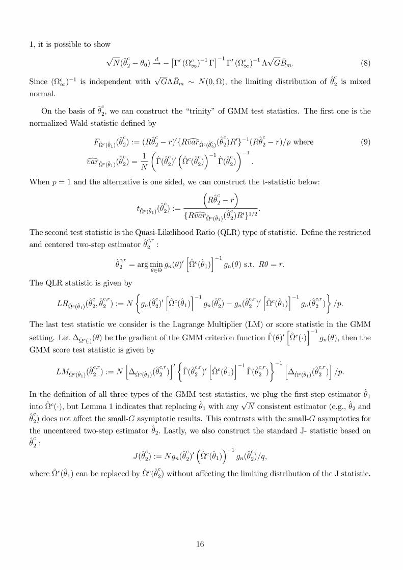
normalized Wald statistic defined by

FΩc(θ1)(θc

2) := (Rθc

2 − r)′RvarΩc(θc2)(θ

c

2)R′−1(Rθc

2 − r)/p where (9)

varΩc(θ1)(θc

2) =1

N

(Γ(θ

c

2)′(

Ωc(θc

2))−1

Γ(θc

2)

)−1

.

When p = 1 and the alternative is one sided, we can construct the t-statistic below:

tΩc(θ1)(θc

2) :=

(Rθ

c

2 − r)

RvarΩc(θ1)(θc

2)R′1/2.

The second test statistic is the Quasi-Likelihood Ratio (QLR) type of statistic. Define the restricted

and centered two-step estimator θc,r

2 :

θc,r

2 = arg minθ∈Θ

gn(θ)′[Ωc(θ1)

]−1

gn(θ) s.t. Rθ = r.

The QLR statistic is given by

LRΩc(θ1)(θc

2, θc,r

2 ) := N

gn(θ

c

2)′[Ωc(θ1)

]−1

gn(θc

2)− gn(θc,r

2 )′[Ωc(θ1)

]−1

gn(θc,r

2 )

/p.

The last test statistic we consider is the Lagrange Multiplier (LM) or score statistic in the GMM

setting. Let ∆Ωc(·)(θ) be the gradient of the GMM criterion function Γ(θ)′[Ωc(·)

]−1

gn(θ), then the

GMM score test statistic is given by

LMΩc(θ1)(θc,r

2 ) := N[∆Ωc(θ1)(θ

c,r

2 )]′

Γ(θc,r

2 )′[Ωc(θ1)

]−1

Γ(θc,r

2 )

−1 [∆Ωc(θ1)(θ

c,r

2 )]/p.

In the definition of all three types of the GMM test statistics, we plug the first-step estimator θ1

into Ωc(·), but Lemma 1 indicates that replacing θ1 with any√N consistent estimator (e.g., θ2 and

θc

2) does not affect the small-G asymptotic results. This contrasts with the small-G asymptotics for

the uncentered two-step estimator θ2. Lastly, we also construct the standard J- statistic based on

θc

2 :

J(θc

2) := Ngn(θc

2)′(

Ωc(θ1))−1

gn(θc

2)/q,

where Ωc(θ1) can be replaced by Ωc(θc

2) without affecting the limiting distribution of the J statistic.

16

Using (8) and Lemma 1, we have FΩc(θ1)(θc

2)d→ F2∞ where

F2∞ = G[R(Γ′ΛS−1ΓΛ

)−1Γ′ΛS−1Bm

]′ [R(Γ′ΛS−1ΓΛ

)−1R′]−1

(10)

×[R(Γ′ΛS−1ΓΛ

)−1Γ′ΛS−1Bm

]/p.

When p = 1, we get tΩc(θ1)(θc

2)d→ T2∞ with

T2∞ =R(Γ′ΛS−1ΓΛ

)−1Γ′ΛS−1

√GBm√

R(Γ′ΛS−1ΓΛ

)−1R′

.

Also, it follows in a similar way that

J(θc

2)d→ J∞ := G

Bm − ΓΛ

(Γ′ΛS−1ΓΛ

)−1Γ′ΛS−1Bm

′S−1 (11)

×Bm − ΓΛ

(Γ′ΛS−1ΓΛ

)−1Γ′ΛS−1Bm

/q.

The remaining question is whether the above representations for F2∞ and J∞ are free of nuisanceparameters. The following proposition provides a positive answer.

Proposition 4. Let Assumptions 1∼6 hold and define Spp·q = Spp − SpqS−1qq Sqp.

(a) FΩc(θ1)(θc

2)d→ G

(Bp − SpqS−1

qq Bq

)′ S−1pp·q(Bp − SpqS−1

qq Bq

)′/p

d= F2∞;

(b) tΩc(θ1)(θc

2)d→√G(Bp − SpqS−1

qq Bq

)/√Spp·q

d= T2∞ for p = 1;

(c) LRΩc(θ1)(θc

2, θc,r

2 ) = FΩc(θ1)(θc

2) + op(1);

(d) LMΩc(θ1)(θc,r

2N) = FΩc(θ1)(θc

2) + op(1);

(e) J(θc

2)d→ (G/q)B′qS−1

qq Bqd= J∞.

To simplify the representations of F2∞ and T2∞ in the above proposition, we note that

G

[Spp SpqSqp Sqq

]d=

G∑g=1

(Bp+q,g − Bp+q

) (Bp+q,g − Bp+q

)′,

where Bp+q,g := (B′p,g, B′p,g)′. The above random matrix has a standard Wishart distribution

Wp+q(G − 1, Ip+q). It follows from the well-known properties of a Wishart distribution that

Spp·q ∼Wp(G− 1− q, Ip)/G and Spp·q is independent of Spq and Sqq.3 Therefore, if we condition on∆ := SpqS−1

qq

√GBq, the limiting distribution F2∞ satisfies

G− p− qG

F2∞d=G− p− q

G

(√GBp + ∆)′Spp·q(

√GBp + ∆)

pd= Fp,G−p−q

(‖∆‖2) , (12)

where Fp,G−p−q(‖∆‖2) is a noncentral F distribution with random noncentrality parameter ‖∆‖2 .

3See Proposition 7.9 in Bilodeau and Brenner.

17

Similarly, the limiting distribution T2∞ can be represented as√G− 1− q

GT2∞

d=

√G− 1− q

G

√GBp + ∆√Spp·q

d= tG−1−q(∆), (13)

which is a noncentral t distribution with a noncentrality parameter ∆. The nonstandard limiting

distributions are similar to those in Sun (2014) which provides the fixed-smoothing asymptotic

result in the case of the series LRV estimation. However, in our setting of clustered dependence,

the scale adjustment and degrees of freedom parameter in (12) and (13) are different from those in

Sun (2014).

The critical values from the nonstandard limiting distribution F2∞ can be obtained through

simulation, but Sun (2014) shows that F2∞ can be approximated by a noncentral F distribution.

With regard to the QLR and LM types of test statistics, Proposition 4-(c) and (d) shows that they

are asymptotically equivalent to FΩc(θ1)(θc

2). This also implies that all three types of test statistics

share the same small-G limit as given in (12) and (13). Similar results are obtained by Sun (2014)

and Hwang and Sun (2015a; 2015b), which focus on two-step GMM estimation and HAR inference

in a time series setting.

For the J-statistic J(θc

2), it follows from Proposition 4-(e) that

G− qG

J(θc

2)d→ J∞

d=G− qG

B′qS−1qq Bq

d= Fq,G−q.

This is consistent with Kim and Sun’s (2012) results except that our adjustment and degrees of

freedom parameter are different.

4 Iterative Two-step and Continuous Updating Schemes

Another class of popular GMM estimators is the continuous updating (CU) estimators, which are

designed to improve the poor finite sample performance of two-step GMM estimators. See Hansen

et al. (1996) and Newey and Smith (2000, 2004) for more discussion on the CU-type estimators.

Here, we consider two types of continuous updating schemes first suggested in Hansen et al. (1996).

The first is motivated by the iterative scheme that updates the FOC of two-step GMM estimation

until it converges. The FOC for θj

IE is

Γ(θj

IE)′Ω−1(θj−1

IE )gn(θj

IE) = 0 for j ≥ 1.

In view of the above FOC, θIE can be regarded as a generalized-estimating-equations (GEE) esti-

mator, which is a class of estimators first studied by Liang and Zeger (1986). When the number of

iterations j goes to infinity until θj

IE converges, we obtain the continuously update GEE estimator

θCU-GEE. The FOC for θCU-GEE is given by

Γ(θCU-GEE)′Ω−1(θCU-GEE)gn(θCU-GEE) = 0. (14)

18

We employ the uncentered CCE, Ω(·) in the definition of θCU-GEE, but it is not diffi cult to show that

Γ(θCU-GEE)′Ω−1(θCU-GEE)gn(θCU-GEE)

= Γ(θCU-GEE)′(

Ωc(θCU-GEE))−1

gn(θCU-GEE) · 1

1 + ν(θCU-GEE)

where

ν(θCU-GEE) = L · gn(θCU-GEE)′(

Ωc(θCU-GEE))−1

gn(θCU-GEE).

Since 1/(1 + ν(θCU-GEE)) is always positive, the first-order condition in (14) holds if and only if

Γ(θCU-GEE)′[Ωc(θCU-GEE)

]−1

gn(θCU-GEE) = 0 (15)

which indicates that the recentering CCE weight in (14) has no effect on the iteration GMM

estimator.

The second CU scheme continuously updates the GMM criterion function, which leads to the

familiar continuous updating GMM (CU-GMM) estimator:

θCU = arg minθ∈Θ

gn(θ)′Ω−1(θ)gn(θ).

Although we use the uncentered CEE Ω(θ) in the above definition, the original definition of θCU in

Hansen, Heaton and Yaron (1996) is based on the centered CCE weighting matrix Ωc(θ). It is easy

to show that

LΩgn(θ)−1(θ)gn(θ) = Lgn(θ)′Ω−1(θ)[Ω(θ)− Lgn(θ)gn(θ)′

] [Ωc(θ)

]−1

gn(θ)

= Lgn(θ)′(

Ωc(θ))−1

gn(θ)

1− Lgn(θ)′Ω−1(θ)gn(θ).

So we have

Lgn(θ)′(

Ωc(θ))−1

gn(θ) =Lgn(θ)′Ω−1(θ)gn(θ)

1− Lgn(θ)′Ω−1(θ)gn(θ).

The above equation reveals the fact that the CU-GMM estimator will not change if the uncentered

weighting matrix Ω(θ) is replaced by the centered one Ωc(θ), i.e.,

θCU = arg minθ∈Θ

gn(θ)′(

Ωc(θ))−1

(θ)gn(θ). (16)

Similar to the centered two-step GMM estimator, the two CU estimators can be regarded as

having a built-in recentering mechanism. For this reason, the limiting distributions of the two CU

estimators are the same as that of the centered two-step GMM estimator, as is shown below.

Proposition 5. Let Assumptions 1, 3∼6 hold. Assume that θCU-GEE and θCU-GMM are√N consis-

tent. Then√N(θCU-GEE − θ0)

d→ −[Γ′ (Ωc

∞)−1 Γ]−1

Γ′ (Ωc∞)−1 Λ

√GBm,

√N(θCU-GMM − θ0)

d→ −[Γ′ (Ωc

∞)−1 Γ]−1

Γ′ (Ωc∞)−1 Λ

√GBm.

19

The proposition shows that the CU estimators and the centered two-step GMM estimator are

asymptotically equivalent under the small-G asymptotics.

Construct the Wald statistics based on the two CU estimators as follows:

FΩc(θCU-GEE )(θθCU-GEE ) = (RθCU-GEE − r)′RvarΩc(θCU-GEE )(θCU-GEE)R′−1(RθCU-GEE − r)/p

FΩc(θCU )(θθCU ) = (RθCU − r)′RvarΩc(θCU )(θCU)R′−1(RθCU − r)/p

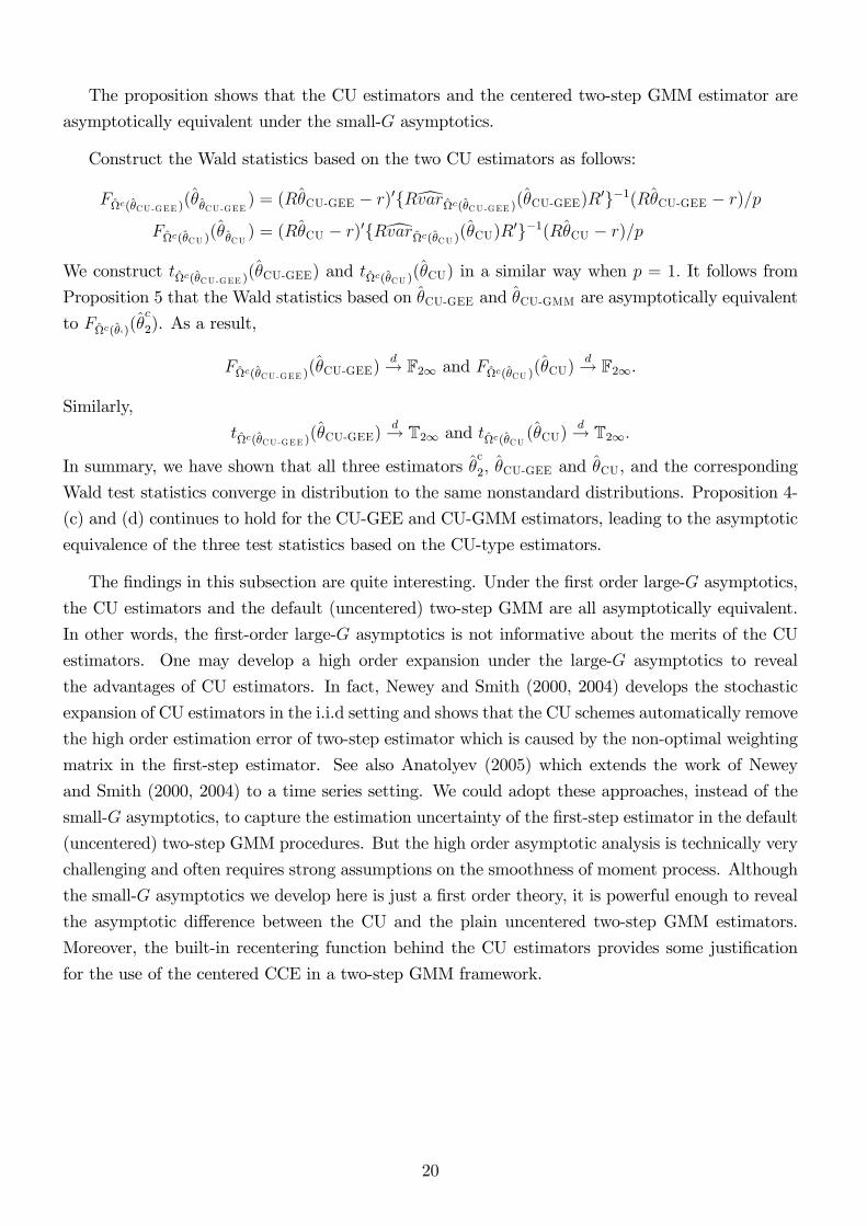
We construct tΩc(θCU-GEE )(θCU-GEE) and tΩc(θCU )(θCU) in a similar way when p = 1. It follows from

Proposition 5 that the Wald statistics based on θCU-GEE and θCU-GMM are asymptotically equivalent

to FΩc(θ‘)(θc

2). As a result,

FΩc(θCU-GEE )(θCU-GEE)d→ F2∞ and FΩc(θCU )(θCU)

d→ F2∞.

Similarly,

tΩc(θCU-GEE )(θCU-GEE)d→ T2∞ and tΩc(θCU (θCU)

d→ T2∞.

In summary, we have shown that all three estimators θc2, θCU-GEE and θCU, and the corresponding

Wald test statistics converge in distribution to the same nonstandard distributions. Proposition 4-

(c) and (d) continues to hold for the CU-GEE and CU-GMM estimators, leading to the asymptotic

equivalence of the three test statistics based on the CU-type estimators.

The findings in this subsection are quite interesting. Under the first order large-G asymptotics,

the CU estimators and the default (uncentered) two-step GMM are all asymptotically equivalent.

In other words, the first-order large-G asymptotics is not informative about the merits of the CU

estimators. One may develop a high order expansion under the large-G asymptotics to reveal

the advantages of CU estimators. In fact, Newey and Smith (2000, 2004) develops the stochastic

expansion of CU estimators in the i.i.d setting and shows that the CU schemes automatically remove

the high order estimation error of two-step estimator which is caused by the non-optimal weighting

matrix in the first-step estimator. See also Anatolyev (2005) which extends the work of Newey

and Smith (2000, 2004) to a time series setting. We could adopt these approaches, instead of the

small-G asymptotics, to capture the estimation uncertainty of the first-step estimator in the default

(uncentered) two-step GMM procedures. But the high order asymptotic analysis is technically very

challenging and often requires strong assumptions on the smoothness of moment process. Although

the small-G asymptotics we develop here is just a first order theory, it is powerful enough to reveal

the asymptotic difference between the CU and the plain uncentered two-step GMM estimators.

Moreover, the built-in recentering function behind the CU estimators provides some justification

for the use of the centered CCE in a two-step GMM framework.

20

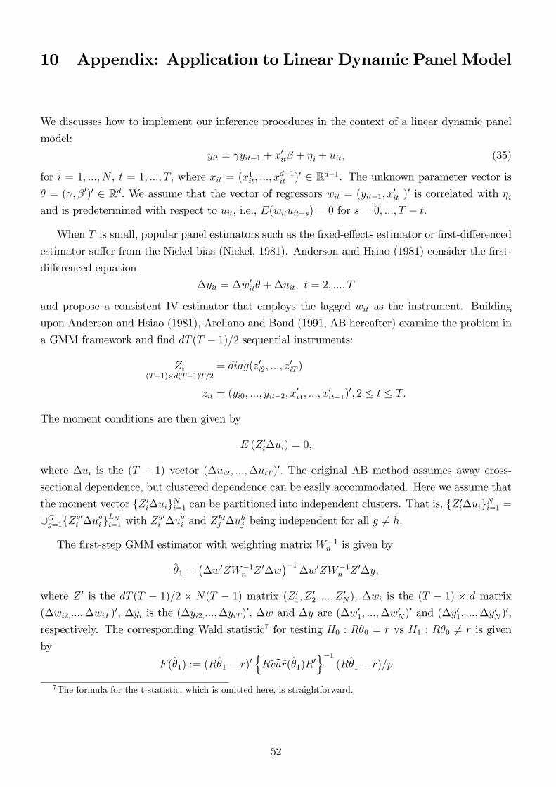
5 Asymptotic F and t tests

Under the small-G asymptotics, the limiting distributions of two-step test statistics, including

Wald, QLR and LM, and the t statistics, are nonstandard and hence critical values have to be

simulated in practice. This contrasts with the conventional large-G asymptotics, where the limiting

distributions are the standard chi-square and normal distributions. In this section, we show that

a simple modification of the two-step Wald and t statistics enables us to develop the standard F

and t asymptotic theory under the small-G asymptotics. The asymptotic F and t tests are more

appealing in empirical applications because the standard F and t distributions are more accessible

than the nonstandard F2∞ and T2∞ distributions.

The modified two-step Wald, QLR and LM statistics are

FΩc(θc2)(θ

c

2) :=G− p− q

G·FΩc(θ

c2)(θ

c

2)

1 + qGJ(θ

c

2), (17)

LRΩc(θ1)(θc

2, θc,r

2 ) :=G− p− q

G·LRΩc(θ1)(θ

c

2, θc,r

2 )

1 + qGJ(θ

c

2),

LM Ωc(θ1)(θc,r

2 ) :=G− p− q

G·LMΩc(θ1)(θ

c,r

2 )

1 + qGJ(θ

c

2),

and the corresponding version of the t-statistic is

tΩc(θc2)(θc

2) :=

√G− 1− q

G·

tΩc(θc2)(θc

2)√1 + q

GJ(θ

c

2).

The modified test statistics involve a scale multiplication factor that uses the usual J-statistic and

a constant factor that adjusts the degrees of freedom.

It follows from Proposition 4 and Theorem 2 that(FΩc(θ

c2)(θ

c

2), J(θc

2))

d→ (F2∞, J∞) (18)

d=(G(Bp − SpqS−1

qq Bq

)′ S−1pp·q(Bp − SpqS−1

qq Bq

)′/p, (G/q)B′qS−1

qq Bq

)(19)

So

FΩc(θc2)(θ

c

2)d→ G− p− q

G

F2∞

1 + qGJ∞

d=G− p− q

pGξ′pS−1

pp·qξp,

where

ξp :=

√G(Bp − SpqS−1

qq Bq)√1 + B′qS−1

qq Bq

.

Similarly,

tΩc(θc2)(θc

2)d→√G− 1− q

G· T2∞√

1 + qGJ∞

d=

ξp√Spp·q

.

In the proof of Theorem 1 we show that ξp follows a standard normal distribution N(0, Ip)

21

and that ξp is independent of S−1pp·q. So the limiting distribution of FΩc(θ

c2)(θ

c

2) is proportional to a

quadratic form in the standard normal vector ξp with an independent inverse-Wishart distributed

weighting matrix S−1pp·q . It follows from a theory of multivariate statistics that the limiting distri-

bution of FΩc(θc2)(θ

c

2) is Fp,G−p−q. Similarly, the limiting distribution of tΩc(θc2)(θc

2) is tG−1−q. This is

formalized in the following theorem.

Theorem 1. Let Assumptions 1∼6 hold. Then the modified Wald, QLR and LM all converge in

distribution to Fp,G−p−q. Also, the t statistics has limiting distribution tG−1−q.

Together with the asymptotic equivalence between θc

2, θCU-GEE and θCU-GMM established in

Proposition 5, the proof of Theorem 1 implies that the modified Wald, LR,LM, and t statistics

based on θCU-GEE and θCU-GMM are all asymptotically F and t distributed under the small-G as-

ymptotics. This equivalence relationship is consistent with the recent paper by Hwang and Sun

(2015b) which establishes the asymptotic F and t limit theory of two-step GMM in time series

setting. But our cluster-robust limiting distributions in Theorem 1 are different from Hwang and

Sun (2015b) in terms of the multiplicative adjustment and the degrees of freedom correction.

It follows from the proofs of Theorem 1 and Proposition 4 that√N(θ

c

2 − θ0)d→MN

(0,(Γ′Ω−1Γ

)−1 · (1 + B′qS−1qq Bq)

)(20)

and J(θc

2)d→ (G/q)B′qS−1

qq Bq

holds jointly under small-G asymptotics. Here, MN(0,V) denotes a random variable that follows

a mixed normal distribution with conditional variance V. The random multiplication term (1 +

B′qS−1qq Bq) in (20) reflects the estimation uncertainty of CCE weighting matrix on the limiting

distribution of√N(θ

c

2 − θ0). The small-G limiting distribution in (20) is in sharp contrast to that

of under the conventional large-G asymptotics as the latter completely ignores the variability in the

cluster-robust GMM weighting matrix. By continuous mapping theorem,√N(θ

c

2 − θ0)√1 + (G/q)J(θ

c

2)

d→ N(

0,(Γ′Ω−1Γ

)−1). (21)

and this shows that the J-statistic modification factor in the denominator effectively cancels out

the uncertainty of CCE to recover the limiting distribution of√N(θ

c

2 − θ0) under the conventional

large-G asymptotics. In view of (21), the finite sample distribution of√N(θ

c

2 − θ0) can be well-

approximated by N(0, varΩc(θ1)(θc

2)) where

varΩc(θ1)(θc

2) := varΩc(θ1)(θc

2) ·(

1 +q

GJ(θ

c

2)). (22)

The modification term (1+(q/G)J(θc

2))−1 degenerates to one as G increases so that the two variance

estimates in (22) become close to each other. Thus, the multiplicative term (1 + (q/G)J(θc

2))−1 in

(17) can be regarded as a finite sample modification to the standard variance estimate varΩc(θ1)(θc

2)

under the large-G asymptotics. For more discussions about the role of J-statistic modification, see

Hwang and Sun (2015b) which casts the two-step GMM problems into OLS estimation and inference

22

in classical normal linear regression.

6 Finite Sample Variance Correction

6.1 Centered Two-step GMM Estimation

Define the infeasible two-step GMM estimator with the centered CCE weighting matrix Ωc(θ0):

θc

2 = arg minθ∈Θ

gn(θ)′(

Ωc(θ0))−1

gn(θ).

Then√N(θ

c

2 − θ0) = −[Γ′(

Ωc(θ0))−1

Γ

]−1

Γ′(

Ωc(θ0))−1√

Ngn(θ0) + op(1)

. But we also have

√N(θ

c

2 − θ0) = −[Γ′(

Ωc(θ1))−1

Γ

]−1

Γ′(

Ωc(θ1))−1√

Ngn(θ0) + op(1) (23)

Together with Lemma 1, this implies that√N(θ

c

2 − θ0) =√N(θ

c

2 − θ0) + op (1) .

That is, the estimation error in θ1 has no effect on the asymptotic distribution of√N(θ

c

2 − θ0) in

the first-order asymptotic analysis. However, in finite samples θc

2 does have higher variation than

θc

2, and this can be attributed to the high variation in Ωc(θ1) than Ωc(θ0). To account for this extra

variation, we could develop a higher order asymptotic theory under the small-G asymptotics. But

this is a formidable task that requires new technical machinery and lengthy calculations. Instead,

we keep one additional term in the stochastic expansion of√N(θ

c

2 − θ0) in hopes of developing a

finite sample correction to our asymptotic variance estimator.

To this end, we first introduce the notion of asymptotic equivalence in distribution ξna∼ η

n

for two stochastically bounded sequences of random vectors ξn ∈ R` and ηn ∈ R` when ξn and ηnconverge in distribution to each other. Now under the small-G asymptotics we have:

√N(θ

c

2 − θ0)a∼ −

Γ′[Ωc(θ0)

]−1

Γ

−1

Γ′[Ωc(θ0)

]−1√NgN(θ0) + (E1n + E2n)

√N(θ1 − θ0)

23

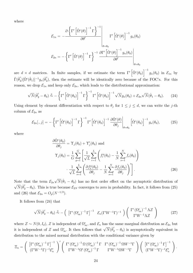
where

E1n = −∂

Γ′[Ωc(θ)

]−1

Γ

−1

∂θ′

∣∣∣∣∣∣∣∣∣θ=θ0

Γ′[Ωc(θ)

]−1

gn(θ0)

E2n = −

Γ′[Ωc(θ)

]−1

Γ

−1 ∂Γ′[Ωc(θ)

]−1

gn(θ0)

∂θ′

∣∣∣∣∣∣∣θ=θ0

are d × d matrices. In finite samples, if we estimate the term Γ′[Ωc(θ0)

]−1

gn(θ0) in E1n by

Γ(θc

2)[Ωc(θ1)]−1gn(θc

2), then the estimate will be identically zero because of the FOC’s. For this

reason, we drop E1n and keep only E2n, which leads to the distributional approximation:

√N(θ

c

2 − θ0)a∼ −

Γ′[Ωc(θ0)

]−1

Γ

−1

Γ′[Ωc(θ0)

]−1√Ngn(θ0) + E2n

√N(θ1 − θ0). (24)

Using element by element differentiation with respect to θj for 1 ≤ j ≤ d, we can write the j-th

column of E2n as

E2n[., j] = −

Γ′[Ωc(θ0)

]−1

Γ

−1

Γ′[Ωc(θ0)

]−1 ∂Ωc(θ)

∂θj

∣∣∣∣∣θ=θ0

[Ωc(θ0)

]−1

gn(θ0), (25)

where

∂Ωc(θ0)

∂θj= Υj(θ0) + Υ′j(θ0) and

Υj(θ0) =1

G

G∑g=1

[1√L

L∑r=1

(f gr (θ0)− 1

N

N∑s=1

fs(θ0)

)

· 1√L

L∑s=1

(∂f gs (θ0)

∂θj− 1

N

N∑s=1

∂fs(θ0)

∂θj

)′]. (26)

Note that the term E2n

√N(θ1 − θ0) has no first order effect on the asymptotic distribution of√

N(θc

2− θ0). This is true because E2N converges to zero in probability. In fact, it follows from (25)

and (26) that E2n = Op(N−1/2).

It follows from (24) that

√N(θ

c

2 − θ0)a∼ −

( [Γ′ (Ωc

∞)−1 Γ]−1 En(Γ′W−1Γ)−1

)( Γ′ (Ωc∞)−1 ΛZ

Γ′W−1ΛZ

)(27)

where Z ∼ N(0, Id), Z is independent of Ωc∞, and En has the same marginal distribution as E2n but

it is independent of Z and Ωc∞. It then follows that

√N(θ

c

2 − θ0) is asymptotically equivalent in

distribution to the mixed normal distribution with the conditional variance given by

Ξn =

( [Γ′ (Ωc

∞)−1 Γ]−1

(Γ′W−1Γ)−1E ′n

)′(Γ′ (Ωc

∞)−1 Ω (Ωc∞)−1 Γ Γ′ (Ωc

∞)−1 ΩW−1Γ

Γ′W−1Ω′ (Ωc∞)−1 Γ Γ′W−1ΩW−1Γ

)( [Γ′ (Ωc

∞)−1 Γ]−1

(Γ′W−1Γ)−1E ′n

).

24

Motivated by the above approximation, we propose to use the following corrected variance

estimator:

varadjΩc(θ1)

(θc

2) =1

NΞn

=1

N

( [Γ′[Ωc(θ1)

]−1

Γ

]−1

En(Γ′W−1n Γ)−1

)

×

Γ′[Ωc(θ1

)]−1

Γ Γ′W−1n Γ

Γ′W−1n Γ Γ′W−1

n Ωc(θ1

)W−1n Γ

×

[Γ′[Ωc(θ1

)]−1

Γ′]−1

(Γ′W−1n Γ)−1E ′n

= varΩc(θ1)(θ

c

2) + EnvarΩc(θ1)(θc

2) + varΩc(θ1)(θc

2)E ′n + Envar(θ1)E ′n (28)

where

En[., j] =

Γ′[Ωc(θ1)

]−1

Γ′−1

Γ′

[Ωc(θ1)

]−1 ∂Ωc(θ)

∂θj

∣∣∣∣∣θ=θ1

[Ωc(θ1)

]−1gn(θ

c

2),

Γ = Γ(θc

2).

The last three terms in (28), which are of smaller order, serve as a finite sample correction to the

original variance estimator.4

Windmeijer (2005), too, has used the idea of variance correction, and his proposed correction

has been widely implemented in applied work for simple models such as linear IV models and lin-

ear dynamic panel data models. However, Windmeijer (2005) considers only an i.i.d. setting, and

there are two principal differences between Windmeijer’s approach and ours. First, our asymptotic

variance estimator involves a centered CCE; in contrast, Windmeijer’s involves only a plain vari-

ance estimator. Second, we consider the small-G asymptotics; Windmeijer (2005) considers the

traditional asymptotics. More broadly, we often have to keep higher-order terms to develop a high

order Edgeworth expansion. Here we choose to focus on variance correction instead of distribution

correction, which is often the real target behind the Edgeworth expansion. In addition to technical

reasons, a principal reason for our choice is that we have already developed more accurate small-G

asymptotic approximations.

With the finite sample corrected variance estimator, we can construct the variance-corrected

Wald statistic:

F adjΩc(θ1)

(θc

2) = (Rθc

2 − r)′[Rvaradj

Ωc(θ1)(θc

2)R′]−1

(Rθc

2 − r)/p. (29)

When p = 1 and for one-sided alternative hypotheses, we can construct the variance-corrected

4Note that the corrected variance estimator is not necessarily larger than the original estimator in finite samples.In the simulation work we consider later, we observe that the smaller value of corrected variance estimate ratherdeteriorates the finite sample performance of variance-corrected statistics. To avoid this undesirable situation, we maymake an adjustment to varadj

Ωc(θ1)(θc

2) so that varadjΩc(θ1)

(θc

2)− varΩc(θ1)(θc

2) is guaranteed to be positive semidefinite.

The adjustment is in a similar spirit with Politis (2011).

25

t-statistic:

tadjΩc(θ1)

(θc

2) =(Rθ

c

2 − r)√RvarcΩc(θ1)(θ

c

2))R′. (30)

Given that the variance correction terms are of smaller order, the variance-corrected statistic will

have the same limiting distribution as the original statistic.

Assumption 7. For each g = 1, ..., G and s = 1, ..., d, define Qgs(θ) as

Qgs(θ) = lim

L→∞E

[1

L

L∑k=1

∂

∂θ′

(∂f gk (θ)

∂θs

)]Then,

supθ∈N (θ0)

∥∥∥∥∥ 1

L

L∑k=1

∂

∂θ′

(∂f gk (θ)

∂θs

)−Qg

s(θ)

∥∥∥∥∥ p→ 0.

holds for each g = 1, ..., G and s = 1, ..., d where N (θ0) is an open neighborhood of θ0 and ‖·‖ is theEuclidean norm. Also, Qg

s(θ0) = Qs(θ0) for g = 1, ...G.

This assumption trivially holds if the moment conditions are linear in parameters.

Theorem 2. Let Assumptions 1∼7 hold. Then

F adjΩc(θ1)

(θc

2) = FΩc(θ1)(θc

2) + op(1) and

tadjΩc(θ1)

(θc

2) = tΩc(θ1)(θc

2) + op(1).

In the proof of Theorem 2, we show that En = (1 + op(1))E2n. That is, the high order correction

term has been consistently estimated in a relative sense. This guarantees that En is a reasonableestimator for E2n, which is of order op(1).

As a direct implication of Theorem 2, the small-G asymptotic distributions of F cΩc(θ1)

(θc

2) and

tcΩc(θ1)

(θc

2) are

F adjΩc(θ1)

(θc

2)d→ F2∞ and t

adjΩc(θ1)

(θc

2)d→ T2∞.

6.2 CU Estimation

For the CU-GEE estimator, we have the following expansion√N(θCU-GEE − θ0)

= −(

Γ′(

Ωc(θ0))−1

Γ

)−1

Γ′(

Ωc(θ0))−1√

Ngn(θ0) + E2n

√N(θCU-GEE − θ0) + op (1) . (31)

This can be regarded as a special case of (24) wherein the first-step estimator θ1 is replaced by the

CU-GEE estimator. So

√N(θCU-GEE − θ0)

a∼ − (Id − E2n)−1

(Γ′(

Ωc(θ0))−1

Γ

)−1

Γ′(

Ωc(θ0))−1√

Ngn(θ0). (32)

26

We can obtain the same expression for the CU-GMM estimator√N(θCU-GMM − θ0).

In view of the representation in (32), the corrected variance estimator for the CU type estimators

can be constructed as follows:

varadjΩc(θCU-GEE )

(θCU-GEE) =(Id − ECU-GEE

)−1

var(θCU-GEE

)(Id − E ′CU-GEE

)−1

varadjΩc(θCU-GEE )

(θCU-GMM) =(Id − ECU-GMM

)−1

var(θCU-GMM

)(Id − E ′CU-GMM

)−1

where

ECU-GEE[., j] =

Γ′[Ωc(θCU-GEE)

]−1

Γ′−1

× Γ′

[Ωc(θCU-GEE)

]−1 ∂Ωc(θCU-GEE)

∂θj

[Ωc(θCU-GEE)

]−1gn(θCU-GEE)

and ECU-GMM is defined in the same way but with θCU-GEE replaced by θCU-GMM. With the finite

sample corrected and adjusted variance estimators in place, the test statistics based on all three

estimators θc

2, θCU-GEE and θCU-GMM converge in distribution to the same nonstandard distributions.

A multiplicative modification provided in Section 5 can then turn the nonstandard distributions

F2∞ and T2∞ into standard F and t distributions.

7 Simulation Evidence

7.1 Design

This section compares the finite sample performance of our new tests by focusing on the following

linear dynamic panel data model.

yit = γyit−1 + x1,itβ1 + x2,itβ2 + x3,itβ3 + ηi + uit.

The unknown parameter vector is θ = (γ, β1, β2, β3) and the corresponding covariates are wit =

(yit−1, xit)′ with xit = (x1,it, x2,it, x3,it)

′. The true value of θ is chosen as θ0 = (0.5, 1, 1, 1). We

denote sgit = (sg1,it, ..., sgk,it)

′ as any vector valued observations in cluster g, and stack all observations

at same period by cluster to define s(g),t = (sg1t, ..., sgLt)′. The j-th predetermined regressor xgj,it are

generated according to the following process:

xgj,it = ρxgj,it−1 + ηgi + ρugit−1 + egj,it

for j = 1, 2, 3, i = 1, ..., L, and t = 1, ..., T . We characterize the within-cluster dependence in η(g),

e(g),t and u(g),t by spatial locations that are indexed by a one-dimensional lattice. Define Ση and Σu

to be L× L matrices whose (i, j)-th elements are σηij = λ|i−j| and σuij = λ|i−j|, respectively, and Σe

to be a 3L× 3L block diagonal matrix with diagonal matrix Σd,e of size L×L for d = 1, ..., 3. The

(i, j)-th element of Σd,e is σed,ij = λ|i−j| for d = 1, ..., 3. The parameter λ governs the degree of spatial

27

dependence in each cluster. When λ = 0, there is no clustered dependence and our model reduces

to that of Windmeijer (2005) which considers a static panel data model with only one regressor.

The individual fixed effects and shocks in group g are generated by:

η(g) ∼ i.i.d.N(0,Ση), vec(e(g),t) ∼ i.i.d.N(0,Σe), (33)

u(g),t = τ tΣ1/2u (δg1ω

g1t, , .., δ

gLω

gLt)′,

δgi ∼ i.i.d.U [0.5, 1.5], and ωgit ∼ i.i.d.χ21 − 1

for i = 1, ..., LN and t = 1, ..., T where τ t = 0.5 + 0.1(t − 1). The DGP of individual shock u(g),t

in (33) features a non-Gaussian process which is heteroskedastic over both time t and individual i.

Also, the clustered dependence structure implies

η(g), vec(e(g),t), δ(g), ω(g),tz ⊥ η(h), vec(e(h),t), δ(h), ω(h),t

for g 6= h at any t and s.

Before we draw an estimation sample for t = 1, ..., T , 50 initial values are generated with

τ t = 0.5 for t = −49, ..., 0, xgd,i,−49 ∼i.i.d.N(ηgi /(1 − ρ), (1 − ρ)−1Σd,e) for d = 1, ..., 3, and ygi,−49 =

(∑3

d=1 xd,i,−49βd + ηgi + ugi,−49)/(1− γ). We fix the values of λ and ρ at 0.75 and 0.70, respectively;

thus each observation is reasonably persistent with respect to both time and spatial dimensions.

We set the number of time periods to be T = 4. In Appendix, we describe how to implement

our new inference procedures in the context of linear dynamic panel model. The parameters are

estimated by the first differenced GMM (AB estimator). The initial first-step estimator with Wn =

(1/N)∑N

i=1 Z′iHZi where H is a matrix that consists with 2’s on the main diagonal, with -1’s

on the main diagonal, and zeros elsewhere. With all possible lagged instruments, the number of

moment conditions for the AB estimator is dT (T − 1)/2 = 24 and the degrees of over-identification

is q = 20. It could be better to use only a subset of full moment conditions because using this full

set of instruments may lead to poor finite sample properties, especially when the number of clusters

G is small. Thus, we also employ a reduced set of instruments; that is, we use the most recent lag

zit = (yit−2, x′it−1)′, leading to d(T − 1) = 12 moment conditions.

7.2 Choice of tests

We focus on theWald type of tests as the Monte Carlo results for other types of tests are qualitatively

similar. We examine the empirical size of a variety of testing procedures, all of which are based on

first-step or two-step GMM estimators. For the first-step procedures, we consider the unmodified

F-statistic F1 := F1(θ1) and the degrees-of-freedom modified F-statistic [(G− p) /G]F1 where the

associated critical values are χ1−αp /p and F1−α

p,G−p, respectively. These two tests have the same size-

adjusted power, because the modification only involves a constant multiplier factor.

For the two-step GMM estimation and related tests, we examine five different procedures. The

first three tests use different test statistics but the same critical value χ1−αp /p. The first test

28

uses the “plain”F-statistic F2 := FΩc(θ1)(θc

2) as defined in (9). The second test uses the statistic

[(G− p− q) /G] ·F2 where (G− p− q) /G is the degree-of-freedom correction factor. The third testuses F2 := FΩc(θ1)(θ

c

2) as defined in (17). Note that

F2 =(G− p− q)

G· F2

1 + (q/G)J(θc

2).

Compared to the second test statistic, F2 has the additional J-statistic correction factor (1 +

(q/G)J(θc

2))−1. The three tests use increasingly more sophisticated test statistics. Because [(G− p− q) /G]→1 and (1 + (q/G)J(θ

c

2))−1 → 1 as G → ∞, both corrections can be regarded as devices for finitesample improvement under the large-G asymptotics.

Table 1: Summary of the first-step, two-step tests, and J test

First-step GMM testsstatistic d.f. adj. F1−α

p,G−p · ·F1 − − − −

G−pGF1 Y Y − −

Two-step GMM testsstatistic d.f. adj. J-modification F1−α

p,G−p−q variance correction

F2 − − − −G−p−qG

F2 Y − − −F2 Y Y − −F2 Y Y Y −

Fadj+ Y Y Y YJ-tests

statistic d.f. adj. F1−αq,G−q · ·

J − − − −G−qGJ c Y Y − −

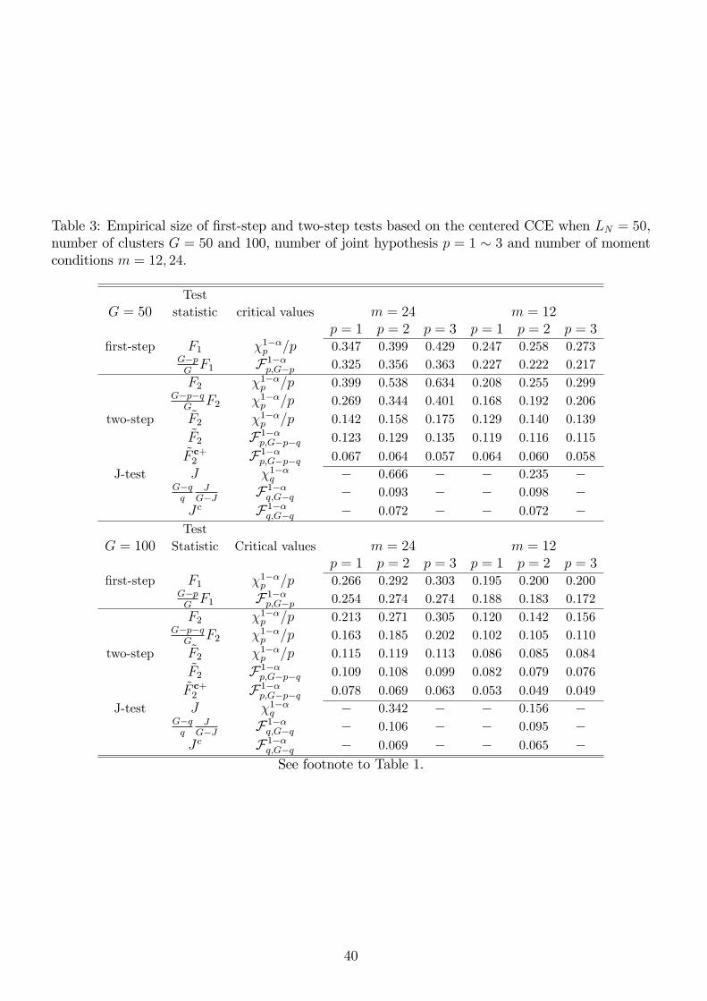
Notes: The first-step tests are based on the first-step GMM estimator θ1. They use the associated F-statistic F1= F 1(θ1) with critical value χ1−α

p /p or F 1−αp,G−p. The first J test employs the statistic J(θ2)

and critical value χ1−αq , and the second J test employs the statistic G−q

G Jc = G−qG J(θ

c

2) and critical

value F1−αq,G−q. All two-step tests are based on the centered two-step GMM estimator θ

c

2 but use different

test statistics and critical values: the unmodified F-statistic F2 = FΩc(θ1)(θc

2), J-statistic and degrees-of-

freedom corrected statistic F2 = FΩc(θ1)(θc

2), and J-statistic, degrees-of-freedom, and finite-sample-variance

corrected F-statistic Fadj+2 = Fadj+Ωc(θ1)

(θc

2), coupled with critical value χ1−αp /p or F1−α

p,G−p−q.

29

Figure 1: Emprical size of the first-step and two-step tests when G = 50, L = 50, q = 20, and p = 3with the nominal size 5% (green line).

The last two tests employ the new F critical values which are justified from the small-G asymptotics.

The fourth test uses the same statistic F2 as the third test but employs the F critical value F1−αp,G−p−q

instead. The fifth test uses the most refined version of the F-statistic F adj as defined in (29) and

the same F critical value F1−αp,G−p−q employed in the fourth test. A summary of the tests considered

is given in Table 1.

7.3 Results

7.3.1 Balanced Cluster Size

We first consider the case when all clusters have an equal number of individuals and take different

values of G ∈ 30, 35, 50, 100 and L ∈ 50, 100. The null hypotheses of interests are

H01 : β10 = 1

H02 : β10 = β20 = 1

H03 : β10 = β20 = β30 = 1

with the corresponding number of joint hypotheses p = 1, 2 and 3, respectively, and the significance

level is 5%. The number of simulation replications is 5000.

Tables 2∼5 report the empirical size of the first-step and two-step tests for different values ofG ∈ 30, 35, 50, 100 and L = 50, 100. The results indicate that both the first-step and two-step tests based on unmodified statistics F1 and F2 suffer from severe size distortions, when the

conventional chi-square critical values are used. For example, with G = 50, L = 50, and p = 3,

30

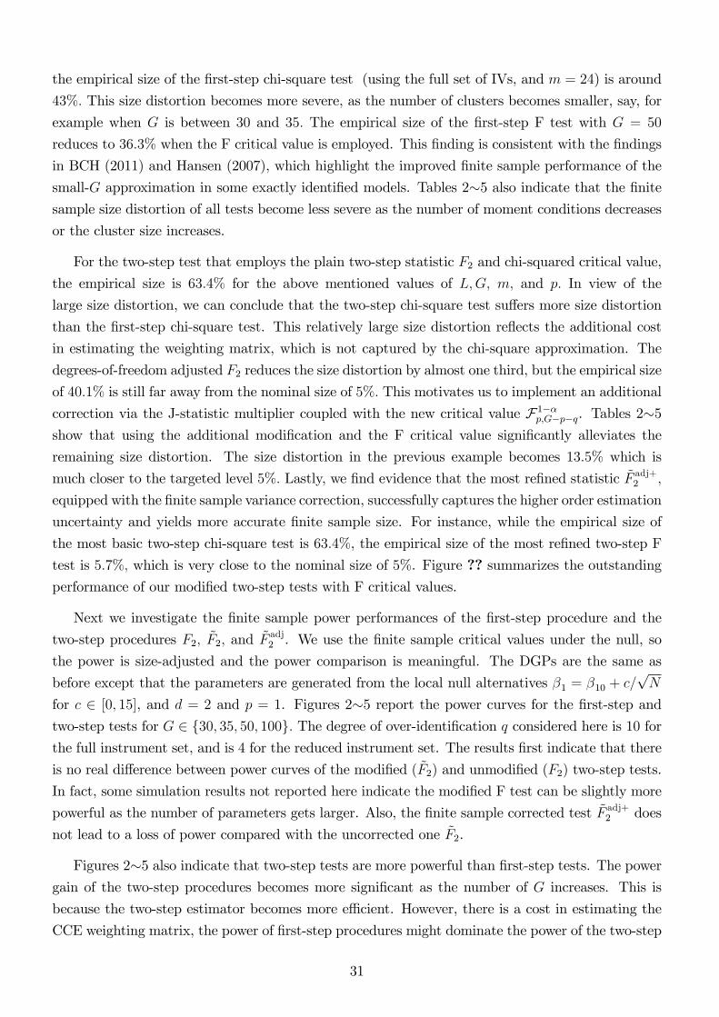
the empirical size of the first-step chi-square test (using the full set of IVs, and m = 24) is around

43%. This size distortion becomes more severe, as the number of clusters becomes smaller, say, for

example when G is between 30 and 35. The empirical size of the first-step F test with G = 50

reduces to 36.3% when the F critical value is employed. This finding is consistent with the findings

in BCH (2011) and Hansen (2007), which highlight the improved finite sample performance of the

small-G approximation in some exactly identified models. Tables 2∼5 also indicate that the finitesample size distortion of all tests become less severe as the number of moment conditions decreases

or the cluster size increases.

For the two-step test that employs the plain two-step statistic F2 and chi-squared critical value,

the empirical size is 63.4% for the above mentioned values of L,G, m, and p. In view of the

large size distortion, we can conclude that the two-step chi-square test suffers more size distortion

than the first-step chi-square test. This relatively large size distortion reflects the additional cost

in estimating the weighting matrix, which is not captured by the chi-square approximation. The

degrees-of-freedom adjusted F2 reduces the size distortion by almost one third, but the empirical size

of 40.1% is still far away from the nominal size of 5%. This motivates us to implement an additional

correction via the J-statistic multiplier coupled with the new critical value F1−αp,G−p−q. Tables 2∼5

show that using the additional modification and the F critical value significantly alleviates the

remaining size distortion. The size distortion in the previous example becomes 13.5% which is

much closer to the targeted level 5%. Lastly, we find evidence that the most refined statistic F adj+2 ,

equipped with the finite sample variance correction, successfully captures the higher order estimation

uncertainty and yields more accurate finite sample size. For instance, while the empirical size of

the most basic two-step chi-square test is 63.4%, the empirical size of the most refined two-step F

test is 5.7%, which is very close to the nominal size of 5%. Figure ?? summarizes the outstandingperformance of our modified two-step tests with F critical values.

Next we investigate the finite sample power performances of the first-step procedure and the

two-step procedures F2, F2, and Fadj2 . We use the finite sample critical values under the null, so

the power is size-adjusted and the power comparison is meaningful. The DGPs are the same as

before except that the parameters are generated from the local null alternatives β1 = β10 + c/√N

for c ∈ [0, 15], and d = 2 and p = 1. Figures 2∼5 report the power curves for the first-step andtwo-step tests for G ∈ 30, 35, 50, 100. The degree of over-identification q considered here is 10 for

the full instrument set, and is 4 for the reduced instrument set. The results first indicate that there

is no real difference between power curves of the modified (F2) and unmodified (F2) two-step tests.

In fact, some simulation results not reported here indicate the modified F test can be slightly more

powerful as the number of parameters gets larger. Also, the finite sample corrected test F adj+2 does

not lead to a loss of power compared with the uncorrected one F2.

Figures 2∼5 also indicate that two-step tests are more powerful than first-step tests. The powergain of the two-step procedures becomes more significant as the number of G increases. This is

because the two-step estimator becomes more effi cient. However, there is a cost in estimating the

CCE weighting matrix, the power of first-step procedures might dominate the power of the two-step

31

ones in other scenarios, i.e., when the cost of employing CCE weighting matrix outweighs the benefit

of estimating it. Some simulation results not reported here show that the power of the first-step

test can be higher than that of a two-step test when the number of parameters d and the number

of joint hypotheses p are large.

Lastly, Tables 2∼5 show that the finite sample size distortion of the (centered) J test and thetransformed (uncentered) J test is substantially reduced when we employ F critical values instead

of conventional chi-squared critical values.

In sum, our simulation evidence clearly demonstrates the size accuracy of our most refined F

test regardless of whether the number of clusters G is small or moderate.

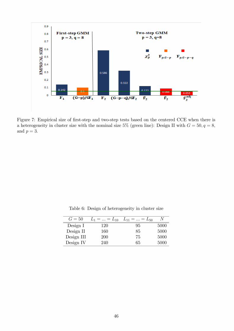
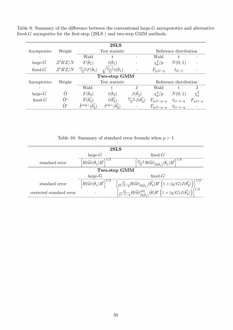
7.3.2 Unbalanced Cluster Size

Although our small-G asymptotics is valid as long as the cluster sizes are approximately equal, we

remain wary of the effect of the cluster size heterogeneity on the quality of the small-G approxi-

mation. In this subsection, we turn to simulation designs with heterogeneous cluster sizes. Each

simulated data set consists of 5, 000. Each simulated data set consists of 5, 000 observations that

are divided into 50 clusters. The sequence of alternative cluster-size designs starts by assigning

120 individuals to each of first 10 clusters and 95 individuals to each of next 40 clusters. In each

succeeding cluster-size design, we subtract 10 individuals from the second group of clusters and add

them to the first group of clusters. In this manner, we construct a series of four cluster-size designs,

in which the proportion of the samples in the first group of clusters grows monotonically from 24%

to 48%. The design is similar to Carter, Schnepel and Steigerwald (2013) which investigates the be-

havior of cluster-robust t-statistic under cluster heterogeneity. Table 6 describes the heterogeneous

cluster-size designs we consider. All other parameter values are the same as before.

Tables 7∼8 report the empirical size of the first-step, two-step, and J tests for q = 20 and p = 3.

The results immediately indicate that the two-step tests suffer from severe size distortion when

the conventional chi-square critical value is employed. For example, under design II, the empirical

size of the “plain”two-step chi-square test is around 60.4% for G = 50, q = 20, and p = 3. The

size distortion become more severe when the degree of heterogeneity across cluster-size increases.

However, our small-G asymptotics still performs very well as they reduce the empirical sizes to

4.3% ∼ 7.9%, which are much closer to the nominal size of 5%. Figures ??∼?? summarize theoutstanding performance of our modified two-step F tests, even with unbalanced cluster sizes. The

results of J tests are omitted here as they are qualitatively similar to those of the F tests.

8 Empirical Application

In this section we employ the proposed procedures to revisit the study of Emran and Hou (2013),

which investigates the casual effects of access to domestic and international markets on household

32

consumption in rural China. They use a survey data of 7998 rural households across 19 provinces

in China. The survey data comes from Chinese Household Income Project (ICPSR 3012) in 1995.5

The regression equation for per capita consumption for household i, Ci, in 1995 (yuan) is specified

as

Ci = α0 + αp + βdAdi + βsA

si + βds(A

di × Asi ) +X ′iβh (34)

+Xv′i βv +Xc′

i βc + εi,

where Adi and Asi are the log distances of access to domestic (km) and international markets (km),

respectively. Xi is the vector of household characteristics that may affect consumption choice, and

Xvi , X

ci are village, county level controls, respectively, which capture the heterogeneity in economic

environments across different regions, and αp is the province level fixed effect.

Among the unknown parameters in vector θ = (α0, αp, β′m, β

′h, β

′v, β

′c)′, our focus of interest

is βm = (βd, βs, βds)′ which measures the casual effect of access to domestic and international

markets on household consumption in the rural areas. To identify these parameters, Emran and

Hou (2013) employs geographic instrumental variables that capture exogenous variations in access

to markets, e.g., straight-line distances to the nearest navigable river and coastline, along with the

topographic and agroclimatic features of the counties.6 There are 21 instrument variables and 31

control variables, including province dummy variables so that the number of moment conditions

m is 52. The number of estimated parameters d is 34, and the degree of over-identification q is

18. Because of the close economic and cultural ties within the same county in rural Chinese areas,

the study clusters the data by the county level and estimates the model using 2SLS and two-step

GMM with uncentered cluster-robust weighting matrix. The data set consists of 7462 observations

divided into 86 clusters where the number of households vary across from a low of 49 to a high of 270.

Statistical inferences in Emran and Hou (2013) are conducted using the large-G asymptotics only.

We apply our more accurate asymptotics to Emran and Hou’s study. The inference methods we use

here are described in Tables 9 and 10 which present the test statistics, the reference distribution,

and the standard error formula (finite sample corrected or not) for each method. Here we view

all corrections, including the degree-of-freedom correction, the J correction, and the finite sample

variance corrections as corrections to the variance estimator.

Table 11 shows the point estimation results, standard error estimates, and associated confidence

intervals (CIs) for each of 2SLS and the uncentered and centered two-step GMM estimators. Similar

to Emran and Hou (2013), our results show that the better access to domestic and international

markets has a substantial positive effect on household consumption, and that the domestic market

effect is significantly higher. For the 2SLS method, there are no much differences in confidence

interval and standard error between the large-G and small-G results. This is well expected because

the number of clusters G = 86 is large enough so that the large-G and small-G approximations are

5The data set is downloadable from the Review of Economics and Statistics website.6For the detailed description of the control variables and instrument variables, see the appendix in Emran and

Hou (2013).

33

close to each other.

The uncentered two-step GMM estimate of the effect of access to domestic market is βd =

−2722.22. The reported standard error 400.5 is about 40% smaller than that of 2SLS. However,

the plain two-step standard error estimate might be downward biased because the variation of the

cluster-robust weighting matrix is not considered. The centered two-step GMM estimator gives a

smaller effect of market access βd = −2670.0 with the modified standard error of 519.2, which is 25%

larger than the plain two-step standard error. However, the modified standard error is still smaller

than that based on the 2SLS method. So the two-step estimator still enjoys the benefit of using

the cluster-robust weighting matrix. The results for other parameters deliver similar qualitative

messages. Table 11 also provides the finite sample corrected standard error estimates of two-step

estimators that capture the extra variation of feasible CCE, leading to slightly larger standard errors

and wider CIs than the uncorrected ones. Overall, our results suggest that the effect of access to

markets may be lower than the previous finding after we take into account the randomness of the

estimated optimal GMM weighting matrix.

9 Conclusion

This paper studies GMM estimation and inference under clustered dependence. To obtain more

accurate asymptotic approximations, we utilize an alternative asymptotics under which the sample

size of each cluster is growing, but the number of cluster size G is fixed. The paper is comprehensive

in that it covers the first-step GMM, the second-step GMM, and continuously-updating GMM

estimators. For the two-step GMM estimator, we show that only if centered moment processes

are used in constructing the weighting matrix can we obtain asymptotically pivotal Wald statistic

and t-statistic. We also find that the centered two-step GMM estimator and CU estimators are

all first-order equivalent under the small-G asymptotics. With the help of the standard J-statistic,

the Wald statistic and t-statistic based on these estimators can be modified to have to standard F

and t limiting distributions. A finite sample variance correction is suggested to further improve the

performance of the asymptotic F and t tests. The advantages of our procedures are clearly reflected

in finite samples as demonstrated by our simulation study and empirical application.

In an overidentified GMM model, the set of moment conditions can be divided into two blocks:

the moment conditions that are for identifying unknown parameters, and the rest of ones for im-

proving the effi ciency of the GMM estimator. We expect that the spatial dependence between these

two blocks of moment conditions is the key information to assess the relative power performance of

first-step and two-step tests. Recently, Hwang and Sun (2015a) compares these two types of tests

by employing more accurate asymptotic approximations in a time series GMM framework. We leave

the extension of this analysis to the spatial setting to future research.

34

References

[1] Anatolyev, S. (2005). “GMM, GEL, serial correlation, and asymptotic bias.”Econometrica,

73(3), 983-1002.

[2] Anderson, T. W. and Hsiao, C. (1981): “Estimation of dynamic models with error compo-

nents.”Journal of the American statistical Association, 76(375), 598-606.

[3] Andrabi, T., Das, J., Khwaja, A. I., and Zajonc, T. (2011). “Do value-added estimates add

value? Accounting for learning dynamics.”American Economic Journal: Applied Economics,

29-54.

[4] Arellano, M. (1987). “Computing Robust Standard Errors for Within-Group Estimators.”Ox-

ford Bulletin of Economics and Statistics, 49, 431-434.

[5] Arellano, M. and Bond, S. (1991): “Some tests of specification for panel data: Monte Carlo

evidence and an application to employment equations.”The Review of Economic Studies, 58(2),

277-297.

[6] Bharath, S., Dittmar, A., and Sivadasan, J. (2013). “Do Going Private Transactions Affect

Plant Productivity?.”Review of Financial Studies, forthcoming.

[7] Bell, R. M., and McCaffrey, D. F. (2002). “Bias reduction in standard errors for linear regression

with multi-stage samples.”Survey Methodology, 28(2), 169-182.

[8] Bertrand, M., Duflo, E., and Mullainathan, S. (2004): “How Much Should We Trust

Differences-in-Differences Estimates?”The Quarterly Journal of Economics, 119(1), 249-275.

[9] Bester, C. A., Conley, T. G., and Hansen, C. B. (2011): “Inference with Dependent Data Using

Cluster Covariance Estimators.”Journal of Econometrics 165(2), 137—151.

[10] Bilodeau, M., and Brenner, D. (2008). “Theory of multivariate statistics.”Springer Science &

Business Media.

[11] Canay, I. A., Romano, J. P., and Shaikh, A. M. (2014). “Randomization tests under an ap-

proximate symmetry assumption.”manuscript, July, 20.

[12] Cameron, A. C., Gelbach, J. B., and Miller, D. L. (2008). “Bootstrap-based improvements for

inference with clustered errors.”Review of Economics and Statistics, 90(3), 414-427.

[13] Cameron, A. C. and Miller, D. L. (2015): “A practitioner’s guide to cluster-robust inference.”

Journal of Human Resources, 50(2), 317-372.

[14] De Brauw, A., and Giles, J. (2012): “Migrant labor markets and the welfare of rural households

in the developing world: Evidence from China.”Working paper.

35

[15] Dube, A., Lester, T. W., and Reich, M. (2010). “Minimum wage effects across state borders:

Estimates using contiguous counties.”Review of economics and statistics, 92(4), 945-964.

[16] Emran, M. S., and Hou, Z. (2013): “Access to markets and rural poverty: evidence from

household consumption in China.”Review of Economics and Statistics, 95(2), 682-697.

[17] Hansen, C. B. (2007): “Asymptotic properties of a robust variance matrix estimator for panel

data when T is large.”Journal of Econometrics, 141(2), 597-620.

[18] Hansen, L. P. (1982): “Large Sample Properties of Generalized Method of Moments Estima-

tors.”Econometrica 50, 1029—1054.

[19] Hayakawa, K. (2014): “Alternative Over-identifying Restriction Test in GMM with Grouped

Moment Conditions.”Working paper.

[20] Hansen, L. P., Heaton, J. and Yaron, A. (1996): “Finite-sample properties of some alternative

GMM estimators.”Journal of Business & Economic Statistics, 14(3), 262-280.

[21] Hwang, J. and Y. Sun (2015a): “Should We Go One Step Further? An Accurate Comparison of

One-Step and Two-Step Procedures in a Generalized Method of Moments Framework”Working

paper, Department of Economics, UC San Diego.

[22] Hwang, J. and Y. Sun.(2015b): “Asymptotic F and t Tests in an Effi cient GMM Setting.”

Working paper, Department of Economics, UC San Diego.

[23] Ibragimov, R., and Müller, U. K. (2010). “t-Statistic based correlation and heterogeneity robust

inference.”Journal of Business & Economic Statistics, 28(4), 453-468.

[24] Ibragimov, R. and Müller, U.K., (2016). “Inference with few heterogeneous clusters.”Review

of Economics and Statistics, 98(1), 83-96.

[25] Imbens, G.W. and Kolesar, M., (2012). “Robust standard errors in small samples: Some prac-

tical advice.”Review of Economics and Statistics , (0).

[26] Jenish, N., and Prucha, I. R. (2009). “Central limit theorems and uniform laws of large numbers

for arrays of random fields.”Journal of econometrics, 150(1), 86-98.

[27] Jenish, N., and Prucha, I. R. (2012). “On spatial processes and asymptotic inference under

near-epoch dependence.”Journal of econometrics, 170(1), 178-190.

[28] Jiang, J., Luan, Y., & Wang, Y. G. (2007). “Iterative estimating equations: Linear convergence

and asymptotic properties.”The Annals of Statistics, 35(5), 2233-2260.

[29] Kiefer, N. M., Vogelsang, T. J. and Bunzel, H. (2002): “Simple Robust Testing of Regression

Hypotheses” Econometrica 68 (3), 695—714.

36

[30] Kiefer, N. M. and Vogelsang, T. J. (2005): “A New Asymptotic Theory for Heteroskedasticity-

Autocorrelation Robust Tests.”Econometric Theory 21, 1130—1164.

[31] Lee, S. (2014). “Asymptotic refinements of a misspecification-robust bootstrap for generalized

method of moments estimators.”Journal of Econometrics, 178, 398-413.

[32] Liang, K.-Y. and Zeger, S. (1986). “Longitudinal Data Analysis Using Generalized Linear

Models.”Biometrika 73(1):13—22.

[33] MacKinnon, James G., and Matthew D. Webb. "Wild bootstrap inference for wildly different

cluster sizes." Journal of Applied Econometrics (2016).

[34] Moulton, B. R. (1990): “An illustration of a pitfall in estimating the effects of aggregate

variables on micro units.”Review of Economics and Statistics, 334-338.

[35] Müller, U. K. (2007). “A theory of robust long-run variance estimation.” Journal of Econo-

metrics, 141(2), 1331-1352.

[36] Newey, Whitney K., and Richard J. Smith. (2000). “Asymptotic bias and equivalence of GMM

and GEL estimators.”Mimeo, MIT.

[37] Newey, Whitney K., and Richard J. Smith. (2004) “Higher order properties of GMM and

generalized empirical likelihood estimators.”Econometrica 72, no. 1 : 219-255.

[38] Nickell, S. (1981). “Biases in dynamic models with fixed effects.”Econometrica: Journal of the

Econometric Society, 1417-1426.

[39] Obstfeld, M., Shambaugh, J. C., and Taylor, A. M. (2008). “Financial stability, the trilemma,

and international reserves (No. w14217).”National Bureau of Economic Research.

[40] Pepper, J. V. (2002). “Robust inferences from random clustered samples: an application using

data from the panel study of income dynamics.”Economics Letters, 75(3), 341-345.

[41] Politis, D. N. (2011). “Higher-order accurate, positive semidefinite estimation of large-sample

covariance and spectral density matrices.”Econometric Theory, 27(04), 703-744.

[42] Shah, B. V., Holt, M. M., and Folsom, R. E. (1977). “Inference about regression models from

sample survey data.”Bulletin of the International Statistical Institute, 47(3), 43-57.

[43] Samila, S., and Sorenson, O. (2011). “Venture capital, entrepreneurship, and economic growth.

The Review of Economics and Statistics.”, 93(1), 338-349.

[44] Stock, J. H. and Watson, M. W. (2008), “Heteroskedasticity-Robust Standard Errors for

Fixed Effects Panel Data Regression.” Econometrica, 76: 155—174. doi: 10.1111/j.0012-

9682.2008.00821.x

37

[45] Sun, Y. (2013): “A Heteroskedasticity and Autocorrelation Robust F Test Using Orthonormal

Series Variance Estimator.”Econometrics Journal 16(1), 1—26.

[46] Sun, Y. (2014): “Fixed-smoothing Asymptotics in a Two-step GMM Framework.”Economet-

rica 82(6), 2327—2370.

[47] Sun, Y., and Kim, M. S. (2012). “Simple and powerful GMM over-identification tests with

accurate size.”Journal of Econometrics, 166(2), 267-281.

[48] Sun, Y., and Kim, M. S. (2015). “Asymptotic F-Test in a GMM Framework with Cross-

Sectional Dependence.”Review of Economics and Statistics, 97(1), 210-223.

[49] Sun, Y., Phillips, P. C. B. and Jin, S. (2008). “Optimal Bandwidth Selection in

Heteroskedasticity-Autocorrelation Robust Testing.”Econometrica 76(1), 175—94.

[50] Webb, M. D. (2014): “Reworking Wild Bootstrap Based Inference for Clustered Errors,”

Queen’s Economics Department Working Paper.

[51] White, H. (1984). “Asymptotic theory for econometricians.”Academic press.

[52] Windmeijer, F. (2005): “A finite sample correction for the variance of linear effi cient two-step

GMM estimators.”Journal of Econometrics, 126(1), 25—51.

[53] Wooldridge, J. M. (2003): “Cluster-sample methods in applied econometrics.”American Eco-

nomic Review, 133—138.

38

Table 2: Empirical size of first-step and two-step tests based on the centered CCE when LN = 50,number of clusters G = 30 and 35, number of joint hypothesis p = 1 ∼ 3 and number of momentconditions m = 12, 24.

TestG = 30 statistic critical values m = 24 m = 12

p = 1 p = 2 p = 3 p = 1 p = 2 p = 3first-step F1 χ1−α

p /p 0.374 0.475 0.528 0.274 0.302 0.332G−pGF1 F1−α

p,G−p 0.333 0.389 0.417 0.236 0.232 0.220F2 χ1−α

p /p 0.659 0.857 0.939 0.308 0.415 0.492G−p−qG

F2 χ1−αp /p 0.414 0.562 0.658 0.229 0.276 0.308

two-step F2 χ1−αp /p 0.128 0.159 0.192 0.147 0.164 0.182

F2 F1−αp,G−p−q 0.087 0.082 0.079 0.124 0.128 0.129

F c+2 F1−αp,G−p−q 0.015 0.015 0.012 0.063 0.063 0.058

J-test J χ1−αq − 0.935 − − 0.329 −

G−qq

JG−J F1−α

q,G−q − 0.069 − − 0.086 −G−qGqJ c F1−α

q,G−q − 0.129 − − 0.071 −Test m = 24 m = 12

G = 35 Statistic Critical values p = 1 p = 2 p = 3 p = 1 p = 2 p = 3first-step F1 χ1−α

p /p 0.381 0.482 0.538 0.268 0.292 0.316G−pGF1 F1−α

p,G−p 0.348 0.407 0.429 0.236 0.236 0.218F2 χ1−α

p /p 0.572 0.756 0.864 0.292 0.357 0.416G−p−qG

F2 χ1−αp /p 0.366 0.483 0.561 0.199 0.248 0.275

two-step F2 χ1−αp /p 0.145 0.174 0.195 0.143 0.156 0.159

F2 F1−αp,G−p−q 0.111 0.119 0.115 0.128 0.126 0.117

F c+2 F1−αp,G−p−q 0.038 0.034 0.033 0.066 0.060 0.057

J-test J χ1−αq − 0.869 − − 0.307 −

G−qq

JG−J F1−α

q,G−q − 0.080 − − 0.091 −G−qGqJ c F1−α

q,G−q − 0.091 − − 0.073 −See footnote to Table 1.

39

Table 3: Empirical size of first-step and two-step tests based on the centered CCE when LN = 50,number of clusters G = 50 and 100, number of joint hypothesis p = 1 ∼ 3 and number of momentconditions m = 12, 24.

TestG = 50 statistic critical values m = 24 m = 12

p = 1 p = 2 p = 3 p = 1 p = 2 p = 3first-step F1 χ1−α

p /p 0.347 0.399 0.429 0.247 0.258 0.273G−pGF1 F1−α

p,G−p 0.325 0.356 0.363 0.227 0.222 0.217F2 χ1−α

p /p 0.399 0.538 0.634 0.208 0.255 0.299G−p−qG

F2 χ1−αp /p 0.269 0.344 0.401 0.168 0.192 0.206

two-step F2 χ1−αp /p 0.142 0.158 0.175 0.129 0.140 0.139

F2 F1−αp,G−p−q 0.123 0.129 0.135 0.119 0.116 0.115

F c+2 F1−αp,G−p−q 0.067 0.064 0.057 0.064 0.060 0.058

J-test J χ1−αq − 0.666 − − 0.235 −

G−qq

JG−J F1−α

q,G−q − 0.093 − − 0.098 −J c F1−α

q,G−q − 0.072 − − 0.072 −Test

G = 100 Statistic Critical values m = 24 m = 12p = 1 p = 2 p = 3 p = 1 p = 2 p = 3

first-step F1 χ1−αp /p 0.266 0.292 0.303 0.195 0.200 0.200

G−pGF1 F1−α

p,G−p 0.254 0.274 0.274 0.188 0.183 0.172F2 χ1−α

p /p 0.213 0.271 0.305 0.120 0.142 0.156G−p−qG

F2 χ1−αp /p 0.163 0.185 0.202 0.102 0.105 0.110

two-step F2 χ1−αp /p 0.115 0.119 0.113 0.086 0.085 0.084

F2 F1−αp,G−p−q 0.109 0.108 0.099 0.082 0.079 0.076

F c+2 F1−αp,G−p−q 0.078 0.069 0.063 0.053 0.049 0.049

J-test J χ1−αq − 0.342 − − 0.156 −

G−qq

JG−J F1−α

q,G−q − 0.106 − − 0.095 −J c F1−α

q,G−q − 0.069 − − 0.065 −See footnote to Table 1.

40

Table 4: Empirical size of first-step and two-step tests based on the centered CCE when LN = 50,number of clusters G = 30 and 35, number of joint hypothesis p = 1 ∼ 3 and number of momentconditions m = 12, 24.

TestG = 30 Statistic Critical values m = 24 m = 12

p = 1 p = 2 p = 3 p = 1 p = 2 p = 3first-step F1 χ1−α

p /p 0.344 0.402 0.440 0.249 0.117 0.289G−pGF1 F1−α

p,G−p 0.300 0.328 0.333 0.217 0.208 0.195F2 χ1−α

p /p 0.610 0.798 0.883 0.275 0.347 0.436G−p−qG

F2 χ1−αp /p 0.371 0.517 0.612 0.191 0.220 0.246

two-step F2 χ1−αp /p 0.101 0.130 0.164 0.116 0.117 0.124

F2 F1−αp,G−p−q 0.061 0.064 0.059 0.095 0.088 0.124

F c+2 F1−αp,G−p−q 0.017 0.015 0.013 0.045 0.043 0.040

J-test J χ1−αq − 0.930 − − 0.336 −

G−qq

JG−J F1−α

q,G−q − 0.073 − − 0.098 −G−qGqJ c F1−α

q,G−q − .114 − − 0.077 −Test m = 24 m = 12

G = 35 Statistic Ref.dist. p = 1 p = 2 p = 3 p = 1 p = 2 p = 3first-step F1 χ1−α

p /p 0.321 0.373 0.393 0.237 0.257 0.269G−pGF1 F1−α

p,G−p 0.292 0.303 0.300 0.213 0.207 0.187F2 χ1−α

p 0.522 0.697 0.826 0.224 0.301 0.362G−p−qG

F2 χ1−αp /p 0.306 0.411 0.484 0.162 0.196 0.224

two-step F2 χ1−αp 0.105 0.125 0.136 0.107 0.115 0.118

F2 F1−αp,G−p−q 0.079 0.079 0.076 0.090 0.090 0.087

F c+2 F1−αp,G−p−q 0.038 0.032 0.026 0.049 0.049 0.044

J-test J χ1−αq − 0.853 − − 0.288 −

G−qq

JG−J F1−α

q,G−q − 0.080 − − 0.098 −G−qGqJ c F1−α

q,G−q − 0.078 − − 0.075 −See footnote to Table 1.

41

Table 5: Empirical size of first-step and two-step tests based on the centered CCE when LN = 50,number of clusters G = 50 and 100, number of joint hypothesis p = 1 ∼ 3 and number of momentconditions m = 12, 24.

TestG = 50 Statistic Critical values m = 24 m = 12

p = 1 p = 2 p = 3 p = 1 p = 2 p = 3first-step F1 χ1−α

p /p 0.269 0.305 0.324 0.206 0.214 0.222G−pGF1 F1−α

p,G−p 0.250 0.260 0.257 0.189 0.180 0.175F2 χ1−α

p /p 0.341 0.469 0.575 0.176 0.211 0.250G−p−qG

F2 χ1−αp /p 0.209 0.268 0.324 0.129 0.146 0.164

two-step F2 χ1−αp /p 0.099 0.115 0.125 0.094 0.098 0.105

F2 F1−αp,G−p−q 0.088 0.091 0.093 0.086 0.083 0.084

F c+2 F1−αp,G−p−q 0.059 0.056 0.052 0.057 0.052 0.055

J-test J χ1−αq − 0.629 − − 0.221 −

G−qq

JG−J F1−α

q,G−q − 0.087 − − 0.094 −J c F1−α

q,G−q − 0.064 − − 0.063 −Test

G = 100 Statistic Critical values m = 24 m = 12p = 1 p = 2 p = 3 p = 1 p = 2 p = 3

first-step F1 χ1−αp /p 0.185 0.203 0.209 0.149 0.147 0.152

G−pGF1 F1−α

p,G−p 0.176 0.185 0.182 0.143 0.136 0.128F2 χ1−α

p /p 0.168 0.225 0.258 0.100 0.120 0.129G−p−qG

F2 χ1−αp /p 0.125 0.149 0.161 0.082 0.089 0.093

two-step F2 χ1−αp /p 0.085 0.091 0.094 0.069 0.073 0.071

F2 F1−αp,G−p−q 0.081 0.082 0.083 0.065 0.067 0.064

F c+2 F1−αp,G−p−q 0.067 0.065 0.064 0.056 0.055 0.051

J-test J χ1−αq − 0.293 − − 0.135 −

G−qq

JG−J F1−α

q,G−q − 0.081 − − 0.081 −J c F1−α

q,G−q − 0.055 − − 0.053 −See footnote to Table 1.

42

0 5 10 15

Pow

er

0

0.1

0.2

0.3

0.4

0.5

0.6

0.7

0.8

0.9

1

0 5 10 15

Pow

er0

0.1

0.2

0.3

0.4

0.5

0.6

0.7

0.8

0.9

Figure 2: Size-adjusted power of the first-step (2SLS) and two-step tests with G = 30 and LN = 50.

0 5 10 15

Pow

er

0

0.1

0.2

0.3

0.4

0.5

0.6

0.7

0.8

0.9

1

0 5 10 15

Pow

er

0

0.1

0.2

0.3

0.4

0.5

0.6

0.7

0.8

0.9

Figure 3: Size-adjusted power of first-step (2SLS) and two-step tests with G = 35 and L = 50.

43

0 5 10 15

Pow

er

0

0.1

0.2

0.3

0.4

0.5

0.6

0.7

0.8

0.9

1

0 5 10 15

Pow

er0

0.1

0.2

0.3

0.4

0.5

0.6

0.7

0.8

0.9

Figure 4: Size-adjusted power of first-step (2SLS) and two-step tests with G = 50 and L = 50.

0 5 10 15

Pow

er

0

0.1

0.2

0.3

0.4

0.5

0.6

0.7

0.8

0.9

1

0 5 10 15

Pow

er

0

0.1

0.2

0.3

0.4

0.5

0.6

0.7

0.8

0.9

Figure 5: Size-adjusted power of first-step (2SLS) and two-step tests with G = 100 and L = 50.

44

Figure 6: Empirical size of first-step and two-step tests based on the centered CCE when there isa heterogeneity in cluster size with the nominal size 5% (green line): Design I with G = 50, q = 8,and p = 3.

45

Figure 7: Empirical size of first-step and two-step tests based on the centered CCE when there isa heterogeneity in cluster size with the nominal size 5% (green line): Design II with G = 50, q = 8,and p = 3.

Table 6: Design of heterogeneity in cluster size

G = 50 L1 = ... = L10 L11 = ... = L50 N

Design I 120 95 5000Design II 160 85 5000Design III 200 75 5000Design IV 240 65 5000

46

Figure 8: Empirical size of first-step and two-step tests based on the centered CCE when there is aheterogeneity in cluster size with the nominal size 5% (green line): Design III with G = 50, q = 8,and p = 3.

Figure 9: Empirical size of first-step and two-step tests based on the centered CCE when there is aheterogeneity in cluster size with the nominal size 5% (green line): Design IV with G = 50, q = 20,and p = 3.

47

Table 7: Empirical size of first-step and two-step tests based on the centered CCE when there is aheterogeneity in cluster size: Design I∼II

Design Itest statistic critical values m = 24 m = 12

p = 1 p = 2 p = 3 p = 1 p = 2 p = 3first-step F1 χ1−α

p /p 0.265 0.303 0.322 0.205 0.201 0.217G−pGF1 F1−α

p,G−p 0.246 0.264 0.261 0.186 0.168 0.165F2 χ1−α

p /p 0.335 0.472 0.575 0.153 0.194 0.242G−p−qG

F2 χ1−αp /p 0.209 0.265 0.319 0.118 0.132 0.153

two-step F2 χ1−αp /p 0.095 0.104 0.119 0.086 0.087 0.091

F2 F1−αp,G−p−q 0.082 0.083 0.085 0.074 0.071 0.072

F adj+2 F1−αp,G−p−q 0.054 0.048 0.043 0.046 0.046 0.047

J-test J χ1−αq − 0.632 − − 0.228 −

G−qq

qJG−qJ F1−α

q,G−q − 0.089 − − 0.100 −G−qGqJ c F1−α

q,G−q − 0.067 − − 0.068 −Design II

m = 24 m = 12G = 35 test statistic critical values p = 1 p = 2 p = 3 p = 1 p = 2 p = 3first-step F1 χ1−α

p /p 0.268 0.304 0.323 0.206 0.213 0.220G−pGF1 F1−α

p,G−p 0.250 0.265 0.261 0.193 0.182 0.171F2 χ1−α

p /p 0.361 0.501 0.601 0.160 0.209 0.254G−p−qG

F2 χ1−αp /p 0.231 0.291 0.338 0.124 0.141 0.170

two-step F2 χ1−αp /p 0.112 0.120 0.132 0.088 0.092 0.100

F2 F1−αp,G−p−q 0.097 0.098 0.102 0.079 0.076 0.082

F adj+2 F1−αp,G−p−q 0.063 0.060 0.057 0.053 0.052 0.056

J-test J χ1−αq − 0.638 − − 0.214 −

G−qq

qJG−qJ F1−α

q,G−q − 0.083 − − 0.094 −G−qGqJ c F1−α

q,G−q − 0.081 − − 0.072 −See footnote to Table 1.

48

Table 8: Empirical size of first-step and two-step tests based on the centered CCE when there is aheterogeneity in cluster size: Design III∼IV

Design IIItest statistic critical values m = 24 m = 12

p = 1 p = 2 p = 3 p = 1 p = 2 p = 3first-step F1 χ1−α

p /p 0.276 0.315 0.327 0.203 0.215 0.228G−pGF1 F1−α

p,G−p 0.254 0.276 0.268 0.186 0.186 0.178F2 χ1−α

p /p 0.378 0.532 0.632 0.168 0.222 0.274G−p−qG

F2 χ1−αp /p 0.244 0.323 0.374 0.134 0.164 0.184

two-step F2 χ1−αp /p 0.117 0.132 0.145 0.097 0.109 0.117

F2 F1−αp,G−p−q 0.101 0.107 0.110 0.088 0.091 0.092

F adj+2 F1−αp,G−p−q 0.04 0.057 0.061 0.061 0.062 0.060

J-test J χ1−αq − 0.631 − − 0.213 −

G−qq

qJG−qJ F1−α

q,G−q − 0.076 − − 0.089 −G−qGqJ c F1−α

q,G−q − 0.102 − − 0.079 −Design IV

m = 24 m = 12G = 35 test statistic critical values p = 1 p = 2 p = 3 p = 1 p = 2 p = 3first-step F1 χ1−α

p /p 0.255 0.306 0.327 0.200 0.214 0.226G−pGF1 F1−α

p,G−p 0.232 0.265 0.266 0.180 0.179 0.171F2 χ1−α

p /p 0.397 0.555 0.664 0.185 0.243 0.304G−p−qG

F2 χ1−αp /p 0.264 0.363 0.429 0.139 0.174 0.205

two-step F2 χ1−αp /p 0.131 0.155 0.176 0.104 0.120 0.136

F2 F1−αp,G−p−q 0.115 0.125 0.140 0.094 0.102 0.110

F adj+2 F1−αp,G−p−q 0.075 0.077 0.079 0.062 0.070 0.077

J-test J χ1−αq − 0.621 − − 0.206 −

G−qq

qJG−qJ F1−α

q,G−q − 0.070 − − 0.080 −G−qGqJ c F1−α

q,G−q − 0.151 − − 0.092 −See footnote to Table 1.

49

Table 9: Summary of the difference between the conventional large-G asympototics and alternativefixed-G asympotics for the first-step (2SLS ) and two-step GMM methods.

2SLSAsymptotics Weight Test statistic Reference distribution

· Wald t · Wald t ·large-G Z ′HZ/N F (θ1) t(θ1) · χ2

p/p N(0, 1) ·fixed-G Z ′HZ/N G−p

G F (θ1)√

G−1G t(θ1) · Fp,G−p tG−1 ·

Two-step GMMAsymptotics Weight Test statistic Reference distribution

· Wald t J Wald t J

large-G Ω F (θ2) t(θ2) J(θ2) χ2p/p N(0, 1) χ2

q

fixed-G Ωc F (θc

2) t(θc

2)G−qG J(θ

c

2) Fp,G−p−q tG−1−q Fq,G−qΩc F adj+(θ

c

2) tadj+(θc

2) · Fp,G−p−q tG−1−q ·

Table 10: Summary of standard error formula when p = 1

2SLSlarge-G fixed-G

standard error[Rvar(θ1)R

′]1/2 [

G−1G RvarΩ(θ1)(θ1)R

′]1/2

Two-step GMMlarge-G fixed-G

standard error[Rvar(θ1)R

′]1/2 [

GG−1−qRvarΩ(θ1)(θ

c

2)R′(1 + (q/G)J(θ

c

2))]1/2

corrected standard error ·[

GG−1−qRvar

adjΩ(θ1)

(θ)R′(1 + (q/G)J(θ

c

2))]1/2

50

Table 11: Results for Emran and Hou (2013) data

2SLSVariables Large-G Asymptotics Fixed-G Asymptotics

Domestic market (Adi ) −2713.2 (712.1) −2713.2 (716.8)[−4109.9,−1316.4] [−4138.0,−1288.0]

International market (Asi ) −1993.5 (514.8) −1993.5 (517.9)[−3002.5,−984.4] [−3023.10,−963.8]

Interaction (Adi × Asi ) 345.8 (105.0) 345.8 (105.6)[140.0, 551.7] [135.8, 555.9]

H0 : βd = βs −2.3218 (2.02%) −2.771 (2.26%)

Two-step GMMVariables Large-G Asymptotics Fixed-G Asymptotics

−2722.8 (400.5) −2670.0 (519.2)

Domestic market (Adi ) (520.7)[−3507.7,−1937.9] [−3706.2,−1633.8]

[−3709.2,−1630.7]−2000.2 (344.3) −1981.3 (446.4)

International market (Asi ) (447.7)[−2675.0,−1325.5] [−2872.3,−1090.3]

[−2874.9,−1087.7]362.7 (68.7) 364.1 (89.1)

Interaction (Adi×Asi ) (89.4)

[228.0, 497.3] [186.2, 541.9][187.5, 542.4]

H0 : βd = βs −5.239 (0%) −3.3318 (0%)−3.3217 (0%)

J-statistic (q = 18) 1.1708 (99.8%) 0.3096 (45.83%)

Notes: Standard errors for 2SLS and the weighting matrix for (centered) two-step GMM estimators areclustered at the county level. Numbers in parentheses are standard errors and intervals are 95% confidenceintervals. For hypothesis testing, the numbers in parentheses are P-values.

51

10 Appendix: Application to Linear Dynamic Panel Model

We discusses how to implement our inference procedures in the context of a linear dynamic panel

model:

yit = γyit−1 + x′itβ + ηi + uit, (35)

for i = 1, ..., N , t = 1, ..., T, where xit = (x1it, ..., x

d−1it )′ ∈ Rd−1. The unknown parameter vector is

θ = (γ, β′)′ ∈ Rd. We assume that the vector of regressors wit = (yit−1, x′it )′ is correlated with ηi

and is predetermined with respect to uit, i.e., E(wituit+s) = 0 for s = 0, ..., T − t.

When T is small, popular panel estimators such as the fixed-effects estimator or first-differenced

estimator suffer from the Nickel bias (Nickel, 1981). Anderson and Hsiao (1981) consider the first-

differenced equation

∆yit = ∆w′itθ + ∆uit, t = 2, ..., T

and propose a consistent IV estimator that employs the lagged wit as the instrument. Building

upon Anderson and Hsiao (1981), Arellano and Bond (1991, AB hereafter) examine the problem in

a GMM framework and find dT (T − 1)/2 sequential instruments:

Zi(T−1)×d(T−1)T/2

= diag(z′i2, ..., z′iT )

zit = (yi0, ..., yit−2, x′i1, ..., x

′it−1)′, 2 ≤ t ≤ T.

The moment conditions are then given by

E (Z ′i∆ui) = 0,

where ∆ui is the (T − 1) vector (∆ui2, ...,∆uiT )′. The original AB method assumes away cross-

sectional dependence, but clustered dependence can be easily accommodated. Here we assume that

the moment vector Z ′i∆uiNi=1 can be partitioned into independent clusters. That is, Z ′i∆uiNi=1 =

∪Gg=1Zg′i ∆ugi

LNi=1 with Z

g′i ∆ugi and Z

h′j ∆uhj being independent for all g 6= h.

The first-step GMM estimator with weighting matrix W−1n is given by

θ1 =(∆w′ZW−1

n Z ′∆w)−1

∆w′ZW−1n Z ′∆y,

where Z ′ is the dT (T − 1)/2 × N(T − 1) matrix (Z ′1, Z′2, ..., Z

′N), ∆wi is the (T − 1) × d matrix

(∆wi2,...,∆wiT )′, ∆yi is the (∆yi2,...,∆yiT )′, ∆w and ∆y are (∆w′1, ...,∆w′N)′ and (∆y′1, ...,∆y

′N)′,

respectively. The corresponding Wald statistic7 for testing H0 : Rθ0 = r vs H1 : Rθ0 6= r is given

by

F (θ1) := (Rθ1 − r)′Rvar(θ1)R′

−1

(Rθ1 − r)/p

7The formula for the t-statistic, which is omitted here, is straightforward.

52

where

var(θ1) = N(∆w′ZW−1

n Z ′∆w)−1(

∆w′ZW−1n Ω(θ1)W−1

n Z ′∆w) (

∆w′ZW−1n Z ′∆w

)−1.

Let Z(g) be the L(T − 1) × dT (T − 1)/2 matrix obtained by stacking all Zi’s belonging to

cluster g. Similarly, let ∆u(g) be the L(T −1) stacked vector of the estimated first-differenced errors

∆ui = ∆yi − ∆w′iθ1. Then, in the presence of clustered dependence, the CCE and centered CCE

are constructed as follows:

Ω(θ1) =1

G

G∑g=1

(Z ′(g)∆u(g)√

L

)(Z ′(g)∆u(g)√

L

)′

Ωc(θ1) =1

G

G∑g=1

(Z ′(g)∆u(g)√

L− 1

G

G∑h=1

Z ′(h)∆u(h)√L

)(Z ′(g)∆u(g)√

L− 1

G

G∑h=1

Z ′(h)∆u(h)√L

)′.

Using the centered CCE Ωc(θ1) as the weighting matrix, the two-step GMM estimator θc

2 is

θc

2 =

∆w′Z

[Ωc(θ1)

]−1

Z ′∆w

−1

∆w′Z[Ωc(θ1)

]−1

Z ′∆y,

and the Wald statistic for θc

2 is

FΩc(θ1)(θc

2) := (Rθc

2 − r)′RvarΩc(θ1)(θ2)R′−1(Rθc

2 − r)/p,

varΩc(θ1)(θc

2) = N

∆w′Z

[Ωc(θ1)

]−1

Z ′∆w

−1

.

Under the conventional large-G asymptotics, both F (θ1) and FΩc(θ1)(θc

2) are asymptotically χ2p/p.

Under our small-G asymptotics, we have

F (θ1)d→ G

G− pFp,G−p and

FΩc(θ1)(θc

2)d→ G

G− p− qFp,G−p−q(‖∆‖2) . (36)

In addition to utilizing these new approximations, we suggest a variance correction in order to

capture the higher order effect of θ1 on Ωc(θ1). The finite sample corrected variance is

varcΩc(θ1)(θc

2) = varΩc(θ1)(θc

2) + EnvarΩc(θ1)(θc

2) + varΩc(θ1)(θc

2)E ′n + Envar(θ1)E ′n (37)

where the j-th column is given by

En[., j] = −

∆w′Z[Ωc(θ1)

]−1

Z ′∆w

−1

∆w′Z[Ωc(θ1)

]−1

· ∂Ωc(θ)

∂θj

∣∣∣∣∣θ=θ

[Ωc(θ)

]−1

Z ′∆u2,

∆u2 = ∆y −∆wθc

2

53

and

∂Ωc(θ)

∂θj

∣∣∣∣∣θ=θ1

= Υj(θ1) + Υ′j(θ1),

Υj(θ1) = − 1

G

G∑g=1

(Z ′(g)∆wj,(g)√

Lg− 1

G

G∑h=1

Z ′(h)∆wj,(h)√Lh

)(Z ′(g)∆u(g)√

Lg− 1

G

G∑h=1

Z ′(h)∆u(h)√Lh

)′∆wi

(T−1)×d= (∆w1,i, ...,∆wd,i) and ∆w(g)

LN (T−1)×d= (∆w1,(g), ...,∆wd,(g))

for each j = 1, ..., d. Here, ∆w(g) is a L(T − 1) × d matrix that stacks ∆wiNi=1 belonging to the

group g. The extra adjustment toward a ‘larger’corrected estimator varadj+Ωc(θ1)

(θc

2) directly follows

from (??).

Based on the finite sample corrected variance estimator in (37) and the usual J-statistic, we

construct the modified Wald statistic:

F adjΩc(θ1)

(θc

2) =G− p− q

G

F adj+Ωc(θ1)

(θc

2)

1 + qGJ(θ

c

2)(38)

where

J(θc

2) := Ngn(θc

2)′(

Ωc(θc

2))−1

(θ)gn(θc

2).

From the F limit theory in Section 5, we have

F adjΩc(θ1)

(θc

2)d→ Fp,G−p−q (39)

andG− qG

J(θc

2)d→ Fq,G−q.

Critical values for from the F distribution are readily available from statistical tables.

54

Appendix of Proofs

Proof of Proposition 1. Part (a). For each g = 1, ..., G,

1√L

L∑i=1

f gi (θ1) =1√L

L∑i=1

f gi (θ0) +

∂f gi (θ∗)

∂θ′

[θ1 − θ0

],

where θ∗is between θ1 and θ0. Here, θ

∗may be different for different rows of ∂f gk (θ

∗)/∂θ′. For

notational simplicity, we do not make this explicit. By Assumptions 2 and 5, we have

1√L

L∑i=1

f gi (θ)

=1√L

L∑i=1

f gi (θ0)− 1

L

L∑i=1

∂f gi (θ∗)

∂θ′(Γ′W−1Γ)−1Γ′W−1 1

G

G∑h=1

(1√L

L∑j=1

fhj (θ0)

)+ op (1)

=1√L

L∑i=1

f gi (θ0)− Γg(Γ′W−1Γ)−1Γ′W−1 1

G

G∑h=1

(1√L

L∑i=1

fhi (θ0)

)+ op (1) . (40)

Using Assumptions 4—6, we then have

1√L

L∑i=1

f gi (θ1)

d→ ΛgBm,g − Γg(Γ′W−1Γ)−1Γ′W−1ΛBm

= ΛBm,g − Γ(Γ′W−1Γ)−1Γ′W−1ΛBm

where Bm := G−1∑G

g=1Bm,g. It follows that

Γ(θ1)′W−1N

1√L

L∑i=1

f gi (θ1)

d→ Γ′W−1[ΛBm,g − Γ(Γ′W−1Γ)−1Γ′W−1ΛBm

]= Γ′W−1ΛBm,g − Γ′W−1ΛBm = Γ′W−1Λ

(Bm,g − Bm

).

So, the scaled CCE matrix converges in distribution to a random matrix:

Γ(θ1)′W−1N Ω(θ1)W−1

N Γ(θ1)

=1

G

G∑g=1

(Γ(θ1)′W−1

N

1√L

L∑i=1

f gi (θ1)

)(1√L

L∑j=1

f gj (θ1)W−1N Γ(θ1)

)′

d→ Γ′W−1Λ

1

G

G∑g=1

(Bm,g − Bm

) (Bm,g − Bm

)′(Γ′W−1Λ

)′.

55

Therefore,

NRvar(θ1)R′

=[Γ(θ1)′W−1

n Γ(θ1)]−1 [

Γ(θ1)′W−1n Ω(θ1)W−1

n Γ(θ1)] [

Γ(θ1)′W−1n Γ(θ1)

]−1

= R[Γ′W−1Γ

]−1Γ′W−1Λ

1

G

G∑g=1

(Bm,g − Bm

) (Bm,g − Bm

)′ΛW−1Γ

[Γ′W−1Γ

]−1R′

= R

1

G

G∑g=1

(Bm,g − Bm

) (Bm,g − Bm

)′R′

where R := R [Γ′W−1Γ]−1

Γ′W−1Λ. Also, it follows by Assumption 4 that√N(Rθ1 − r) = −R(Γ′W−1Γ)−1Γ′W−1

√NgN(θ0) + op(1)

= −R(Γ′W−1Γ)−1Γ′W−1 1√G

G∑g=1

(1√L

L∑i=1

f gi (θ0)

)+ op(1)

d→ −R 1√G

G∑g=1

Bm,g = −R√GBm.

Combining the results so far yields:

F (θ1)d→(R√GBm

)′R

1

G

G∑g=1

(Bm,g − Bm

) (Bm,g − Bm

)′R′

−1

R√GBm/p = F1∞.

Define the p × p matrix Λ such that ΛΛ′ = RR′. Then we have the following distributional

equivalence[R√GBm, R 1

G

G∑g=1

(Bm,g − Bm

) (Bm,g − Bm

)′R′

]d=[ √

GΛBp, ΛSppΛ′].

Using this, we get

F1∞d= GB′pS−1Bp/p

as desired for Part (a). Part (b) can be similarly proved.

Proof of Proposition 2. Parts (a), (b) and (c). All three estimators can be represented in thefollowing form

−(Γ′M−1Γ)−1Γ′M−1Λ√GBm + op(1)

for some weighing matrix M which may be random. Let

MΛ = Λ−1M (Λ′)−1 and ΓΛ = Λ−1Γ.

Then

−(Γ′M−1Γ)−1Γ′M−1Λ√GBm = −(ΓΛM

−1Λ ΓΛ)−1ΓΛM

−1Λ

√GBm,

56

Let UΣV ′ be a singular value decomposition (SVD) of ΓΛ. By construction, U ′U = UU ′ = Im,

V ′V = V ′V = Id, and

Σ =

[Ad×d

Oq×d

],

where A is a diagonal matrix. Denoting

M = U ′MΛU =

(M11 M12

M21 M22

),

we have

(ΓΛM−1Λ ΓΛ)−1ΓΛM

−1Λ

=[V Σ′U ′M−1

Λ UΣV ′]−1

V Σ′U ′M−1Λ

=[V Σ′ (U ′MΛU)

−1ΣV ′

]−1

V Σ′ (U ′MΛU)−1U ′

= V(A′M11A

)−1 (A′d×d, O′q×d

)( M11 M12

M21 M22

)U ′

= V A−1(M11)−1(Id, Od×q

)( M11 M12

M21 M22

)U ′

= V A−1(M11)−1(M11, M12

)U ′ = V A−1

(Id, (M11)−1M12

)U ′

= V A−1(Id, −M12M

−122

)U ′.

So

−(ΓΛM−1Λ ΓΛ)−1ΓΛM

−1Λ

√GBm = −V A−1

(Id, −M12M

−122

)U ′√GBm.

For θ1, the matrix M is W , and so

M = W = (ΛU)−1W[(ΛU)−1]′ = ( W11 W12

W21 W22

).

Therefore √N(θ1 − θ0)

d→ −√GV A−1

(Bd − βW Bq

),

where we have used U ′Bmd= Bm = (B′d, B

′q)′ for any orthonormal matrix U.

For θ, the matrix MΛ is S, and so√N(θ2 − θ0)

d→ −[V Σ′U ′M−1

Λ UΣV ′]−1

V Σ′U ′M−1Λ

√GU ′Bm

= −V (ΣU ′S−1UΣ′)−1ΣU ′S−1U√GU ′Bm

d= −V (ΣS−1Σ′)−1ΣS−1

√GBm,

using the asymptotic equivalence (S, Bm)d= (U ′SU,U ′Bm) for any orthonormal matrix U. Therefore,

√N(θ2 − θ0)

d→ −V A−1√G(Bd − βSBq).

57

For the estimator θ2, the matrix MΛ is D∞. We have√N(θ2N − θ0)

d→ −[Γ′ΛD

−1∞ ΓΛ

]−1Γ′ΛD

−1∞√GBm

= −[V Σ′ (U ′D∞U)

−1ΣV ′

]−1

V Σ (U ′D∞U)−1U ′√GBm

= −V[Σ′D−1

∞ Σ]−1

Σ′D−1∞ U

′√GBm

= −V A−1(Id, −D12D−1

22

)U ′√GBm (41)

where

D∞ = U ′D∞U =

D11d×d

D12d×q

D21q×d

D22q×q

.

To investigate each component of D∞ = G−1∑G

g=1 U′DgD

′gU , we first look at the term U ′Dg for

each g = 1, ..., G :

U ′Dg = U ′Bm,g − U ′ΓΛ(Γ′ΛW−1Λ ΓΛ)−1Γ′ΛW

−1Λ Bm

= U ′Bm,g − U ′UΣV ′(Γ′ΛW−1Λ ΓΛ)−1V Σ′U ′W−1

Λ UU ′Bm

= BUm,g − Σ(Σ′U ′W−1

Λ UΣ)−1Σ′U ′W−1Λ UBU

m

where BUm,g = U ′Bm,g and BU

m = U ′Bm. But

BUm,g − Σ(Σ′W−1Σ)−1Σ′W−1BU

m

= BUm,g −

[A

O

](AW 11A)−1

[A O′

]( W 11 W 12

W 21 W 22

)BUm

= BUm,g −

(W 11

)−1

O′

O O

( W 11 W 12

W 21 W 22

)BUm

= BUm,g −

I(W 11

)−1

W 12

O O

BUm

= BUm,g −

[BUd − βW BU

q

O

]= (BU

m,g − BUm) + wBU

q

for

w =

(βWIq

)∈ Rm×q.

58

So, the matrix D∞ can be represented by

D∞ =1

G

G∑g=1

(BUm,g − BU

m + wBUq

) (BUm,g − BU

m + wBUq

)′=

1

G

G∑g=1

(BUm,g − BU

m)(BUm,g − BU

m)′ + wBUq (BU

q )′w′

:= SU∞ + wBUq (BU

q )′w′.

From this, the block matrix components of D∞ are

D11 = SU∞,11 + βW BUq (BU

q )′β′W,

D12 = SU∞,12 + βW BUq (BU

q )′,

D21 = SU∞,21 + BUq (BU

q )′β′W,

D22 = SU∞,22 + BUq (BU

q )′ = SU∞,22. (42)

Using these representations, we can rewrite (41) as√N(θ2 − θ0)

d→ −V A−1(Id, −D12D−1

22

)√GBU

m

= V A−1√G[BUd − D12D−1

22 BUq

]= −V A−1

√G[BUd −

(SU∞,12 + βW B

Uq (BU

q )′) (SU∞,22

)−1BUq

]= −V A−1

√GBUd −

[SU∞,12 − (BU

d − βW BUq )(BU

q )′] (SU∞,22

)−1BUq

d= −V A−1

√G(Bd − βS∞Bq

)− V A−1

√GBd − βW Bq

· (κG/G).

(d) It is easy to check that the weak convergences in (a)∼(c) hold jointly. By continuousmapping theorem we have

√N(θ2 − θ0)−

√N(θ2 − θ0)−

√N(θ1 − θ0) · (κG/G)

d→ 0,

which implies that√N(θ2 − θ0)−

√N(θ2 − θ0)−

√N(θ1 − θ0) · (κG/G) = op (1) .

That is √N(θ2 − θ0) =

√N(θ2 − θ0) +

√N(θ1 − θ0) · (κG/G) + op (1) .

(e) Using the same argument in the proof of Proposition 1, we have

√Ngn(θ2) =

1√G

G∑g=1

(1√L

L∑i=1

f gi (θ2)

)d→ Λ√G(UU ′Bm − ΓΛ

[Γ′ΛD

−1∞ ΓΛ

]−1Γ′ΛD

−1∞ Bm

)d= Λ√G[UBU

m − ΓΛV A−1(BUd − D12D−1

22 BUq

)]

59

with D12 and D22 given in (42). Therefore,

J(θ2) = Ngn(θ2)′(

Ω(θ1))−1

gn(θ2)

d→ GUBU

m − ΓΛV A−1(BUd − D12D−1

22 BUq

)′ × Λ (ΛD∞Λ′)−1

Λ

×UBU

m − ΓΛV A−1(BUd − D12D−1

22 BUq

)= G

BUm − U ′ΓΛV A

−1(BUd − D12D−1

22 BUq

)′U ′D−1

∞ U

×BUm − U ′ΓΛV A

−1(BUd − D12D−1

22 BUq

)= G

BUm −

[Id×d

Oq×d

] (BUd − D12D−1

22 BUq

)′D−1∞

×BUm −

[Id×d

Oq×d

] (BUd − D12D−1

22 BUq

)

= G

(D12D−1

22 BUq

BUq

)′D−1∞

(D12D−1

22 BUq

BUq

)= G(BU

q )′D−122 B

Uq =d GB′qS

−1∞,22Bq = κG,

where the second last equality follows from straightforward calculations. The joint convergence can

be proved easily.

Proof of Proposition 3. It follows from√N(θ2 − θ0)

d→ V A−1√G[BUd − D12D−1

22 BUq

]and Ω(θ1)

d→ ΛD∞Λ′

jointly that

F2,Ω(θ1)(θ2)

=[R(θ2 − θ0)

]′ (RvarΩ(θ1)(θ2)R′

)−1

R(θ2 − θ0)/p

d→ G(BUd − D12D−1

22 BUq )′A−1′V ′R′

[R(

Γ′ (ΛD∞Λ′)−1

Γ)−1

R′]−1

×RV A−1(BUd − D12D−1

22 BUq )/p

= G(BUd − D12D−1

22 BUq )′A−1′V ′R′ ·

R[Γ′ (Λ′)

−1U (U ′D∞U)

−1U ′Λ−1Γ

]−1

R′−1

×RV A−1(BUd − D12D−1

22 BUd )/p

= G(BUd − D12D−1

22 BUq )′A−1′V ′R′

RV A−1D11·2A

−1′V ′R′−1

×RV A−1(BUd − D12D−1

22 BUd )/p.

Let Up×pΣV ′d×d be a SVD of RV A−1, where Σ =

(Ap×p, Op×(d−p)

). By definition, V is the matrix

60

of eigenvectors of (RV A−1)′(RV A−1) . Let

V =

(Vd×d O

O Iq×q

)and define

D=

(D11 D12

D21 D22

)=

(Vd×d O

O Iq

)′(D11 D12

D21 D22

)(Vd×d O

O Iq

)= V′D∞V.

Then

D =1

G

G∑g=1

V′U ′(Bm,g − Bm)(Bm,g − Bm)′VU +

(V ′βWIq

)BUq (BU

q )′

(V ′βWIq

)′

=d 1

G

G∑g=1

(Bm,g − Bm)(Bm,g − Bm)′ +

(V ′βWIq

)BqB

′q

(V ′βWIq

)′,

which implies that

D11 :=

(Dpp Dp,d−pDd−p,p Dd−p,d−p

)d=

1

G

G∑g=1

(Bd,g − Bd)(Bd,g − Bd)′ +(V ′βW

)BqB

′q

(V ′βW

)′, (43)

and

D12 :=

(DpqDd−p,q

)d=

1

G

G∑g=1

(Bd,g − Bd)(Bq,g − Bq)′ +(V ′βW

)BqB

′q. (44)

Now

F2,Ω(θ1)(θ2)

d→ G(BUd − D12D−1

22 BUq )′V Σ′U ′

UΣV ′D11·2V Σ′U ′

−1

UΣV ′(BUd − D12D−1

22 BUq )/p

= G(BUd − D12D−1

22 BUq )′V Σ′ ·

ΣV ′D11·2V Σ′

−1

· ΣV ′(BUd − D12D−1

22 BUq )/p

= G(V ′BUd − D12D−1

22 BUq )′ · Σ′

ΣD11·2Σ′

−1

Σ · (V ′BUd − D12D−1

22 BUq )/p

= G(V ′BUd − D12D−1

22 BUq )′ · Σ′

Σ(D11 − D12D−1

22 D21

)Σ′−1

(V ′BUd − D12D−1

22 BUq )/p

d= G

[Bp − DpqD−1

qq Bq

]′A′A(Dpp − DpqD−1

qq Dqp)A′−1

A[Bp − DpqD−1

qq Bq

]/p

d= G

[Bp − DpqD−1

qq Bq

]′ (Dpp − DpqD−1

qq Dqp)−1 [

Bp − DpqD−1qq Bq

]/p,

where Dpq, Dqq, and Dqp in the last two equalities are understood to equals the correspondingcomponents on the right hand sides of (43) and (44). Here we have abused the notation a little bit.

We have (Dpp DpqD′pq Dqq

)=

(Spp Spq

S ′pq Sqq

)+ wBqB

′qw′ (45)

61

for

w =

(βp

W

Iq

)∈ R(p+q)×q.

We have therefore shown that the first representation of the limit of F2,Ω(θ1)(θ2) holds. Direct

calculations show that the second representation is numerically identical to the first representation.

This completes the proof of Proposition 3.

Proof of Lemma 1. The centered CCE Ωc(θ) can be represented as:

Ωc(θ) =1

G

G∑h=1

1√L

L∑i=1

(fhi (θ)− 1

N

G∑g=1

L∑s=1

f gs (θ)

)

× 1√L

L∑j=1

(fhj (θ)− 1

N

G∑g=1

L∑s=1

f gs (θN)

)′.

To prove Part (a), it suffi ces to show that

1√L

L∑i=1

(fhi (θ)− 1

N

G∑g=1

L∑s=1

f gs (θ)

)(46)

=1√L

L∑i=1

(fhi (θ0)− 1

N

G∑g=1

L∑s=1

f gs (θ0)

)(1 + op(1))

holds for each h = 1, ..., G. By Assumption 3 and using a Taylor expansion, we have

1√L

L∑i=1

fhi (θ) = (1 + op(1))

(1√L

L∑i=1

fhi (θ0) +1

L

L∑i=1

∂fhi (θ)

∂θ′√L(θ − θ0)

)

Using√N(θ − θ0) = Op(1) and Assumption 5, we have

1√L

L∑i=1

fhi (θ) = (1 + op(1))

(1√L

L∑i=1

fhi (θ0) + Γ√L(θ − θ0)

)

for each h = 1, ..., G. That is, the effect of the estimation uncertainty in θ does not change with the

cluster. It then follows that

1√L

L∑i=1

(fhi (θ)− 1

N

G∑g=1

L∑s=1

f gs (θ)

)

= (1 + op(1))

(1√L

L∑i=1

fhi (θ0)− 1

G

G∑g=1

1√L

L∑i=1

f gi (θ0)

),

which completes the proof of part (a).

To prove Part (b), we apply CLT in Assumption 4 together with 6 to obtain:

1√L

L∑i=1

fhi (θ0)− 1

G

G∑g=1

1√L

L∑i=1

f gi (θ0)d→ Λ

(Bm,h − Bm

),

62

where the convergence holds jointly for h = 1, ..., G. As a result,

Ωc(θ)d→ 1

GΛ

G∑g=1

(Bm,g − Bm

) (Bm,g − Bm

)′Λ′.

Proof of Proposition 4. The proof of part (a) is essentially the same as the proof of Proposition 3.

The only difference is that the second term in (45) will not be present for the centered two-step

GMM estimator θc

2. The proof of part (b) is similar. The proof of part (e) is similar to that of

Proposition 2(e).

To prove part (c), recall that the restricted two-step GMM estimator θc,r

2N minimizes

gn(θ)′[Ωc(θ1)

]−1

gn(θ)/2 + λ′n(Rθ − r). (47)

The first order conditions are

Γ(θc,r

2 )[Ωc(θ1)

]−1

gn(θc,r

2 ) +R′λn = 0, (48)

Rθc,r

2 − r = 0.

Using a Taylor expansion and Assumption 3, we can combine two FOC’s to get

√N(θ

c,r

2 − θ0) = −Φ−1Γ′[Ωc(θ1)

]−1√Ngn(θ0) (49)

− Φ−1R′(RΦ−1R′

)−1

RΦ−1Γn′[Ωcn(θ1)

]−1√Ngn(θ0) + op(1),

where Φ := Γ′[Ωcn(θ1)

]−1

Γ. Subtracting (49) from (8), we have

√N(θ

c

2 − θc,r

2 ) = −Φ−1R′(RΦ−1R′

)−1

RΦ−1Γ′[Ωc(θ1)

]−1√Ngn(θ0) + op(1). (50)

By Taylor expansion and Assumption 3 we have

g′n(θc,r

2 ) = g′n(θc

2) + (θc,r

2 − θc

2)′Γ′ + op(N−1/2)

and

Ng′n(θc

2)[Ωc(θ1)

]−1

gn(θc

2)−Ng′n(θc,r

2 )[Ωc(θ1)

]−1

gn(θc

2) (51)

= N(θc

2 − θc,r

2 )′Γ′(θc

2)[Ωc(θ1)

]−1

gn(θ1) +Op

(1√N

)= Op

(1√N

).

Here the last equality follows from the FOC’s for θc

2. In a similar way, we can write the second term

63

in (51) as

Ng′n(θc,r

2 )[Ωc(θ1)

]−1

gn(θc

2)

= Ng′n(θc,r

2 )[Ωc(θ1)

]gn(θ

c,r

2 ) +N(θc

2 − θc,r

2 )′Φ(θc

2 − θc,r

2 ) + op(1).

Combining this and (50), we get

LRΩc(θ1)(θc

2, θc,r

2 )

=

Ngn(θ

c

2)′[Ωc(θ1)

]−1

gn(θc

2)−Ngn(θc,r

2 )′[Ωc(θ1)

]−1

gn(θc,r

2 )

/p

= N(θc,r

2 − θc

2)′Φ(θc,r

2 − θc

2)/p+ op(1)

=√Ng′n(θ0)

[Ωc(θ0)

]−1

ΓΦ−1R′(RΦ−1R′

)−1

RΦ−1Γ′√Ngn(θ0)/p+ op(1)

=√N(Rθ

c

2 − r)′ (

RΦ−1R′)−1√

N(Rθ

c

2 − r)/p+ op(1)

= F2,Ωc(θ1)(θc

2) + op(1).

as desired.

To prove part (d), we rewrite the FOC in (48) as√N∆Ωc(θ1)(θ

c,r

2 ) = −R′√Nλn

= −R′(RΦ−1R′

)−1

RΦ−1Γ′[Ωc(θ1)

]−1√Ngn(θ0) + op(1)

= Φ√N(θc

2 − θc,r

2

)+ op(1).

So,

LMΩc(θ1)(θc,r

2 ) = N[∆Ωc(θ1)(θ

c,r

2 )]′

Φ−1[∆Ωc(θ1)(θ

c,r

2 )]/p

= N(θc

2 − θc,r

2

)′Φ√N(θc

2 − θc,r

2

)/p+ op(1)

= LRΩc(θ1)(θc

2, θc,r

2 ) + op(1)

= F2,Ωc(θ1)(θc

2) + op(1).

Proof of Proposition 5. For the result with CU-GEE estimator θCU-GEE, we have

√N(θCU-GEE − θ0) = −

(Γ′(

Ωc(θCU-GEE))−1

Γ

)−1

Γ′(

Ωc(θCU-GEE))−1√

Ngn(θ0) + op(1).

Since θCU-GEE is√N consistent, we can apply Lemma 1 to obtain Ωc

N(θCU-GEE) = ΩcN(θ0) + op(1).

Invoking the continuous mapping theorem yields√N(θCU-GEE − θ0)

d→ −

Γ′ (Ωc∞)−1 Γ

−1

Γ′ (Ωc∞)−1 Λ

√GBm

as desired.

64

For the CU-GMM estimator, we let Γj(θCU-GMM) be the j-th column of Γj(θCU-GMM). Then, the

FOC with respect to the j-th element of θCU-GMM is

0 = Γj(θCU-GMM)′[Ωc(θCU-GMM)

]−1

gn(θCU-GMM)

− gn(θCU-GMM)′[Ωc(θCU-GMM)

]−1

Υj(θCU-GMM)[Ωc(θCU-GMM)

]−1

gn(θCU-GMM), (52)

where

Υj(θ) =1

N

G∑g=1

(L∑r=1

f gr (θ)

)(L∑s=1

∂fs(θ)

∂θj

)′− LNgN(θ)

(∂gN(θ)

∂θj

)′.

The second term in (52) can be written as

gn(θCU-GMM)′[Ωc(θCU-GMM)

]−1

Υj(θCU-GMM)[Ωc(θCU-GMM)

]−1

gn(θCU-GMM)

=√Lgn(θCU-GMM)′

[Ωc(θCU-GMM)

]−1[

1

G

G∑g=1

(1

L

L∑r=1

f gr (θCU-GMM)

)

·(

1

L

L∑s=1

∂f gs (θCU-GMM)

∂θ

)− 1

G

G∑g=1

(1

L

L∑s=1

∂f gs (θCU-GMM)

∂θ

)′]

·(

Ωc(θCU-GMM))−1√

Lgn(θCU-GMM).

Given that θCU-GMM = θ0 +Op(L−1/2N ), we have

Ωc(θCU-GMM) = Op(1)

√Lgn(θCU-GMM) =

1

G

G∑g=1

(1√L

L∑s=1

f gs (θ0)

)+ Γ√L(θCU-GMM − θ0) + op(1) = Op(1)

1

L

L∑s=1

f gs (θCU-GMM) =1

L

L∑s=1

f gs (θ0) +1

L

L∑s=1

∂f gs (θ)

∂θ(θCU-GMM − θ0) = Op

(1√L

)and for each g = 1, ..., G,(

1

L

L∑r=1

f gr (θCU-GMM)

)(1

L

L∑s=1

∂f gs (θCU-GMM)

∂θ

)

− 1

G

G∑g=1

(1

L

L∑s=1

∂f gs (θCU-GMM)

∂θ

)′

= Op

(1√L

)· op(1) = op

(1√L

).

Combining these together, the second term in FOC in (52) is op(L−1/2N ). As a result,

Γ(θCU-GMM)′[Ωc(θCU-GMM)

]−1

gn(θCU-GMM) = op

(1√L

),

65

and so

√N(θCU-GMM − θ0) = −

Γ′[Ωc(θCU-GMM)

]−1

Γ

−1

Γ′[Ωc(θCU-GMM)

]−1√Ngn(θ0) + op(1)

d→ −

Γ′ (Ωc∞)−1 Γ

−1Γ′ (Ωc

∞)−1 Λ√GBm.

Proof of Theorem 1. Define B′q = (B′q,1, ..., B′q,G)′ and denote

vg =(Bq,g − Bq

)′ [ G∑g=1

(Bq,g − Bq

) (Bq,g − Bq

)′]−1

Bq.

Then, the distribution of√GSpqS

−1qq Bq conditional on Bq can be represented as

√G

(G∑g=1

(Bp,g − Bp

) (Bq,g − Bq

)′)( G∑g=1

(Bq,g − Bq

) (Bq,g − Bq

)′)−1

Bq

=√G

G∑g=1

(Bp,g − Bp

)vg =

√G

G∑g=1

Bp,gvg −√GBp

G∑g=1

vg

d= N

(0, G

G∑g=1

v2g · Ip

)

where the last line holds because∑G

g=1 vg = 0. Note that

GG∑g=1

v2g = G

G∑g=1

(Bq,g − Bq

)′ [ G∑g=1

(Bq,g − Bq

) (Bq,g − Bq

)′]−1

Bq

· B′q

[G∑g=1

(Bq,g − Bq

) (Bq,g − Bq

)′]−1 (Bq,g − Bq

)= GB′q

[G∑g=1

(Bq,g − Bq

) (Bq,g − Bq

)′]−1 [ G∑g=1

(Bq,g − Bq

)×(Bq,g − Bq

)′] [ G∑g=1

(Bq,g − Bq

) (Bq,g − Bq

)′]Bq

= B′q

[G∑g=1

(Bq,g − Bq

) (Bq,g − Bq

)′/G

]−1

Bq

= B′qS−1qq Bq.

So conditional on Bq,√GSpqS

−1qq Bq is distributed as N(0, B′qS

−1qq Bq · Ip). It then follows that the

distribution of√G(Bp − SpqS−1

qq Bq

)conditional on Bq is

√G(Bp − SpqS−1

qq Bq

)∼ N

(0, (1 + B′qS

−1qq Bq) · Ip

)66

using the independence of Bp from SpqS−1qq Bq conditional on Bq. Therefore the conditional distrib-

ution of ξp is

ξp :=

√G(Bp − SpqS−1

qq Bq)√1 + B′qS

−1qq Bq

∼ N(0, Ip).

Given that the conditional distribution of ξp does not depend on Bq, the unconditional distribution

of ξp is also N(0, Ip).

Using ξp ∼ N(0, Ip), Spp·q ∼ G−1Wm(G− q − 1, Ip) and ξp is independent of Spp·q, we have

ξ′p

(GSpp·q

G− q − 1

)−1

ξp ∼ Hotelling’s T 2 distribution T 2p,G−q−1.

It then follows thatG− p− q

p (G− q − 1)ξ′p

(GSpp·q

G− q − 1

)−1

ξp ∼ Fp,G−p−q.

That isG− p− q

pGξ′p

(Spp·q

)−1

ξp ∼ Fp,G−p−q.

Together with Proposition 4(c)(d), this completes the proof of the F limit theory in parts (a), (b)

and (c). The proof of the t limit theory is similar and is omitted here.

Proof of Theorem 2. We first show that En = E2n (1 + op (1)) . For each j = 1, ..., d, we have

En[., j] =

Γ′[Ωc(θ1)

]−1

Γ

−1

Γ′[Ωc(θ1)

]−1 ∂Ωc(θ)

∂θj

∣∣∣∣∣θ=θ1

[Ωc(θ1)

]−1

gn(θc

2)

=

Γ′[Ωc(θ0)

]−1

Γ

−1

Γ′[Ωc(θ0)

]−1 ∂Ωc(θ)

∂θj

∣∣∣∣∣θ=θ1

[Ωc(θ1)

]−1

gn(θc

2)(1 + op(1))

where the second equality holds by Assumption 3, 5 and Lemma 1. Using a Taylor expansion, we

have

gn(θc

2) = gn(θ0)− Γ

Γ′[Ωc(θ0)

]−1

Γ

−1

Γ′[Ωc(θ0)

]−1

gn(θ0)(1 + op(1)).

So

En[., j] =

Γ′[Ωc(θ0)

]−1

Γ

−1

Γ′[Ωc(θ0)

]−1 ∂Ωc(θ)

∂θj

∣∣∣∣∣θ=θ1

[Ωc(θ0)

]−1

gn(θc

2)(1 + op(1))

−

Γ′[Ωc(θ0)

]−1

Γ

−1

Γ′[Ωc(θ0)

]−1 ∂Ωc(θ)

∂θj

∣∣∣∣∣θ=θ1

[Ωc(θ0)

]−1

Γ

×

Γ′[Ωc(θ0)

]−1

Γ

−1

Γ′[Ωc(θ0)

]−1

gn(θ0)

(1 + op(1))

67

for each j = 1, ..., d. For the term, ∂Ωc(θ)∂θj

∣∣∣θ=θ1

, recall that

∂Ωc(θ)

∂θj

∣∣∣∣∣θ=θ1

= Υj(θ1) + Υ′j(θ1),

Υj(θ) =1

N

G∑g=1

[L∑r=1

(f gr (θ)− 1

N

N∑s=1

fs(θ)

)(L∑s=1

(∂f gs (θ)

∂θj− 1

N

N∑s=1

∂fs(θ)

∂θj

))′].

It remains to show that Υj(θ1) = Υj(θ0)(1 + op(1)). From the proof of Lemma 1, we have

1√L

L∑r=1

(f gr (θ1)− 1

N

N∑s=1

fs(θ1)

)

=1√L

L∑r=1

(f gr (θ0)− 1

N

N∑s=1

fs(θ0)

)(1 + op(1)) (53)

for each g = 1, ..., G. By Assumption 3, 7 and a Taylor expansion, we have:

1√L

L∑s=1

∂f gs (θ1)

∂θj=

(1√L

L∑s=1

∂f gs (θ0)

∂θj+

1√L

L∑s=1

∂

∂θ′

(∂f gs (θ0)

∂θj

)√L(θ1 − θ0)

)(1 + op(1))

:=

(1√L

L∑s=1

∂f gs (θ0)

∂θj+Q(θ0)

√L(θ1 − θ0)

)(1 + op(1))

for j = 1, ..., d and g = 1, ..., G. This implies that

L∑s=1

(∂f gs (θ1)

∂θj− 1

N

N∑s=1

∂fs(θ1)

∂θj

)

=L∑s=1

(∂f gs (θ0)

∂θj− 1

N

N∑s=1

∂fs(θ0)

∂θj

)(1 + op(1)) (54)

Combining these together, we have Υ(θ1) = Υ(θ0)(1 + op(1)) from which we obtain the desired

result

En = E2n (1 + op (1)) . (55)

Now, define the infeasible corrected variance

varc,infΩc(θ1)

(θc

2)

= varΩc(θ1)(θc

2) + E2nvarΩc(θ1)(θc

2) + varΩc(θ1)(θc

2)E ′2n + E ′2nvar(θ1)E ′2n

and the corresponding infeasible Wald statistic

Fc2,Ωc(θ1)

(θc

2) = (Rθc

2 − r)′[Rvarc,inf

Ωc(θ1)(θc

2)R′]−1

(Rθ2 − r)/p.

The result in (55) implies

F c2,Ωc(θ1)

(θc

2) = Fc2,Ωc(θ1)

(θc

2)(1 + op(1)).

68

Also, E2n = op(1) and we have

varc,infΩc(θ1)

(θc

2) = varcΩc(θ1)(θc

2)(1 + op(1)),

and so

F c2,Ωc(θ1)

(θc

2) = Fc2,Ωc(θ1)

(θc

2) + op(1)

= F2,Ωc(θ1)(θc

2) + op(1).

69