27
Simple Linear Regression 1
| Date post: | 18-Dec-2015 |
| Category: |
Documents |
| Upload: | russell-fletcher |
| View: | 243 times |
| Download: | 5 times |
1
Simple Linear Regression
2
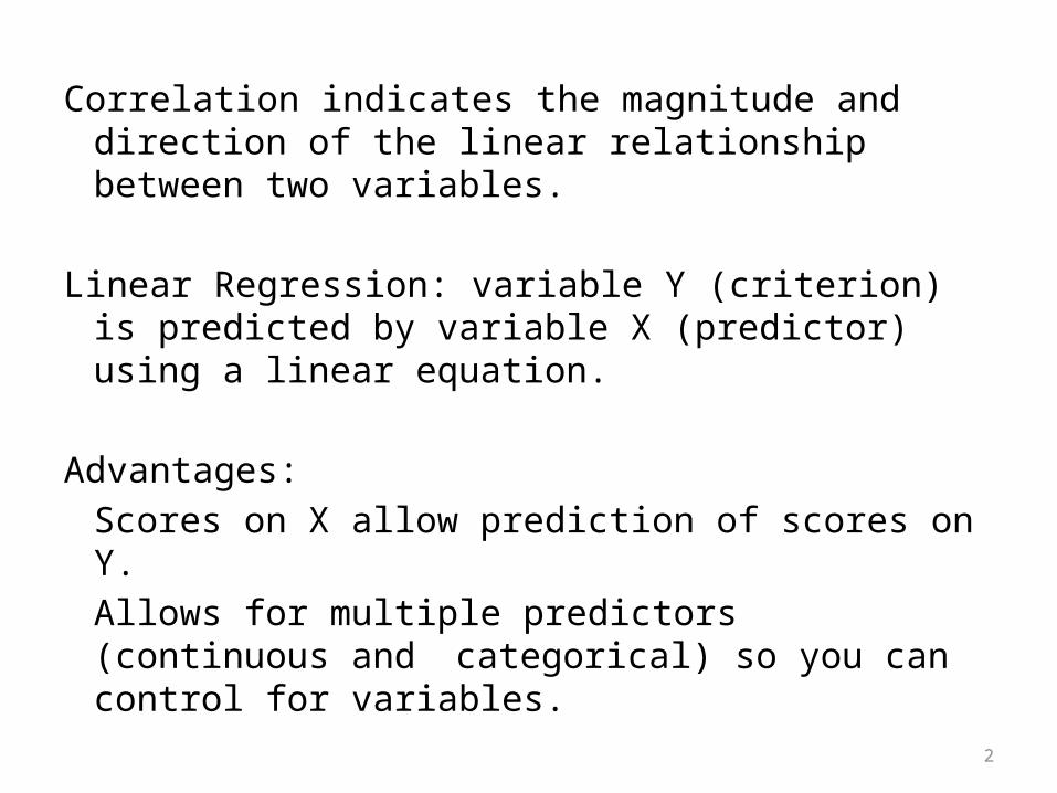
Correlation indicates the magnitude and direction of the linear relationship between two variables.
Linear Regression: variable Y (criterion) is predicted by variable X (predictor) using a linear equation.
Advantages: Scores on X allow prediction of scores on Y. Allows for multiple predictors (continuous and categorical) so you can control for variables.
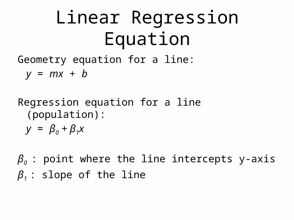
Linear Regression Equation
Geometry equation for a line: y = mx + b
Regression equation for a line (population): y = β0 + β1x
β0 : point where the line intercepts y-axis
β1 : slope of the line
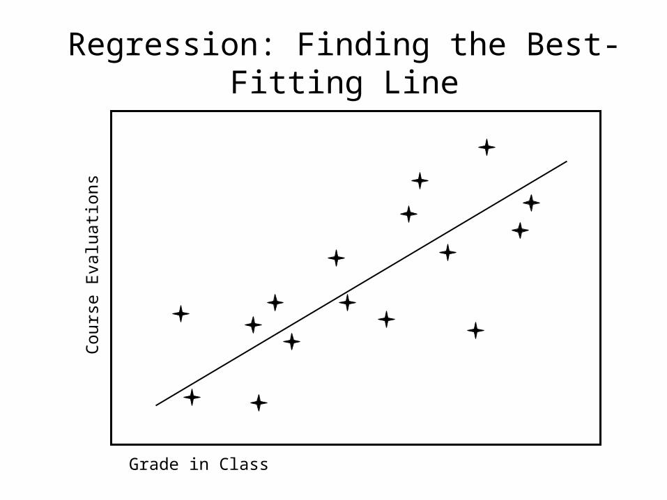
Regression: Finding the Best-Fitting LineCo
urse
Eva
luati
ons
Grade in Class
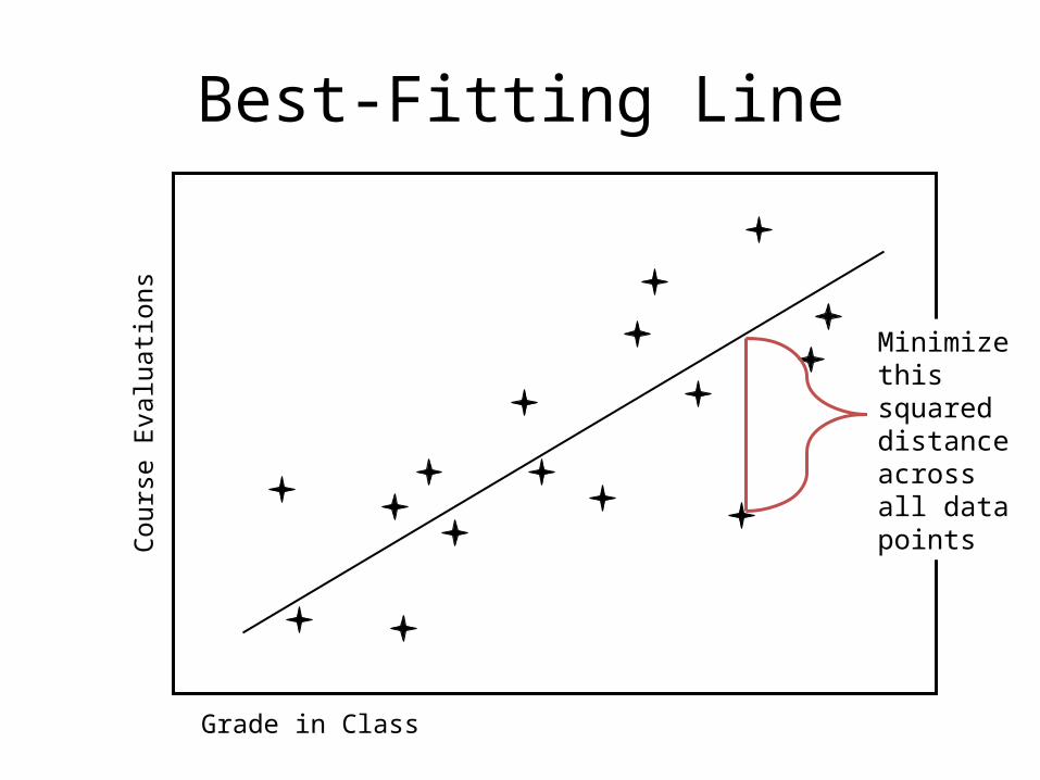
Best-Fitting LineCo
urse
Eva
luati
ons
Grade in Class
Minimize this squared distance across all data points
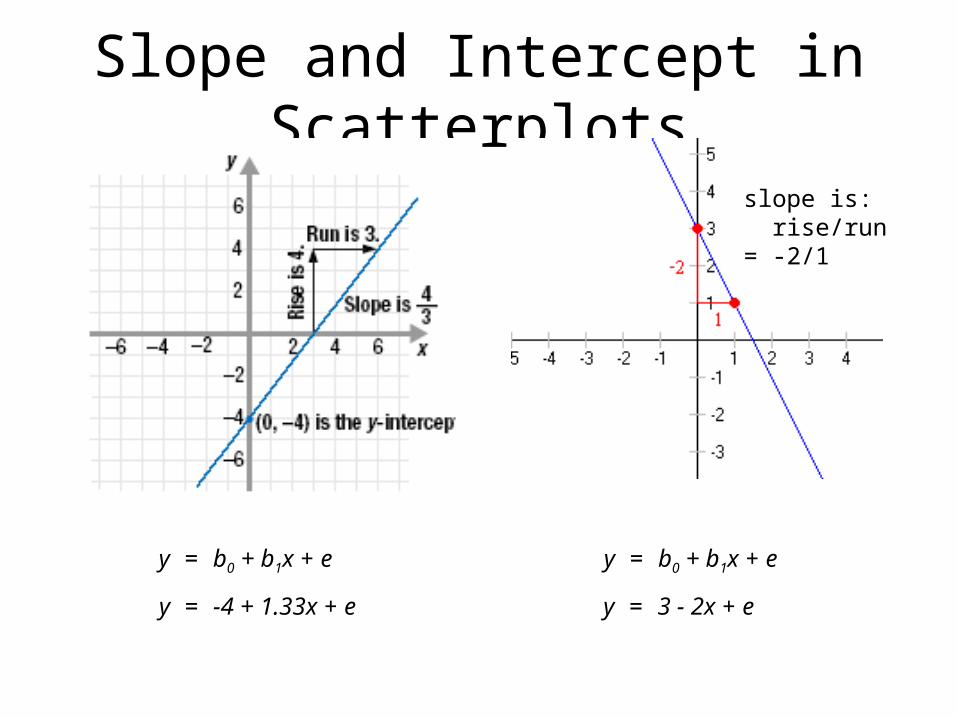
Slope and Intercept in Scatterplots
y = b0 + b1x + e
y = -4 + 1.33x + e
y = b0 + b1x + e
y = 3 - 2x + e
slope is: rise/run = -2/1
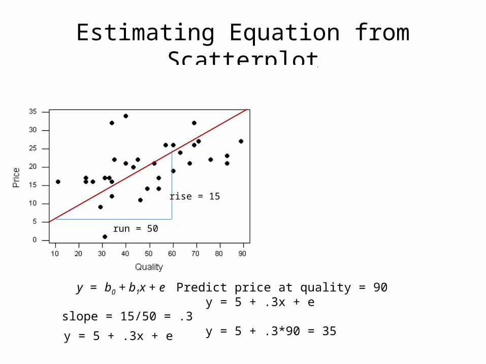
Estimating Equation from Scatterplot
y = b0 + b1x + e
y = 5 + .3x + e
run = 50
rise = 15
slope = 15/50 = .3
Predict price at quality = 90 y = 5 + .3x + e
y = 5 + .3*90 = 35
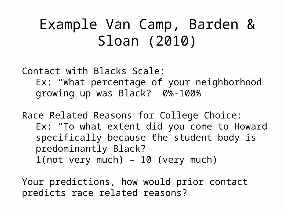
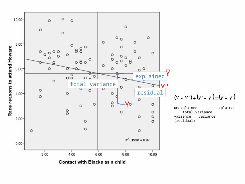
Example Van Camp, Barden & Sloan (2010)
Contact with Blacks Scale: Ex: “What percentage of your neighborhood growing up was Black?” 0%-100%
Race Related Reasons for College Choice: Ex: “To what extent did you come to Howard specifically because the student body is predominantly Black?” 1(not very much) – 10 (very much)
Your predictions, how would prior contact predicts race related reasons?
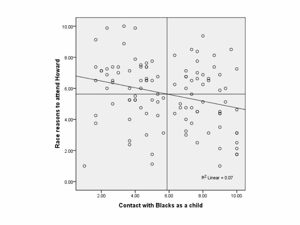
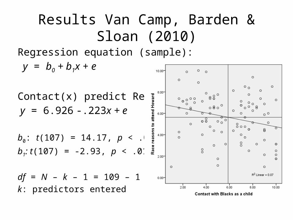
Results Van Camp, Barden & Sloan (2010)
Regression equation (sample): y = b0 + b1x + e
Contact(x) predict Reasons: y = 6.926 -.223x + e
b0: t(107) = 14.17, p < .01
b1: t(107) = -2.93, p < .01
df = N – k – 1 = 109 – 1 – 1 k: predictors entered
Unstandardized and Standardized b
unstandardized b: in the original units of X and Y
tells us how much a change in X will produce a change in Y in the original units (meters, scale points…)
not possible to compare relative impact of multiple predictors
standardized b: scores 1st standardized to SD units
+1 SD change in X produces b*SD change in Yindicates relative importance of multiple predictors of Y
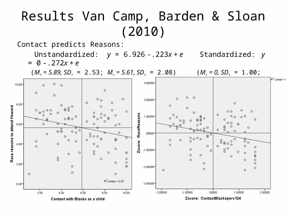
Results Van Camp, Barden & Sloan (2010)Contact predicts Reasons: Unstandardized: y = 6.926 -.223x + e Standardized: y = 0 -.272x + e (Mx = 5.89, SDx = 2.53; My = 5.61, SDy = 2.08) (Mx = 0, SDx = 1.00; My = 0, SDy = 1.00)

save new variables that are standardized versions of current variables
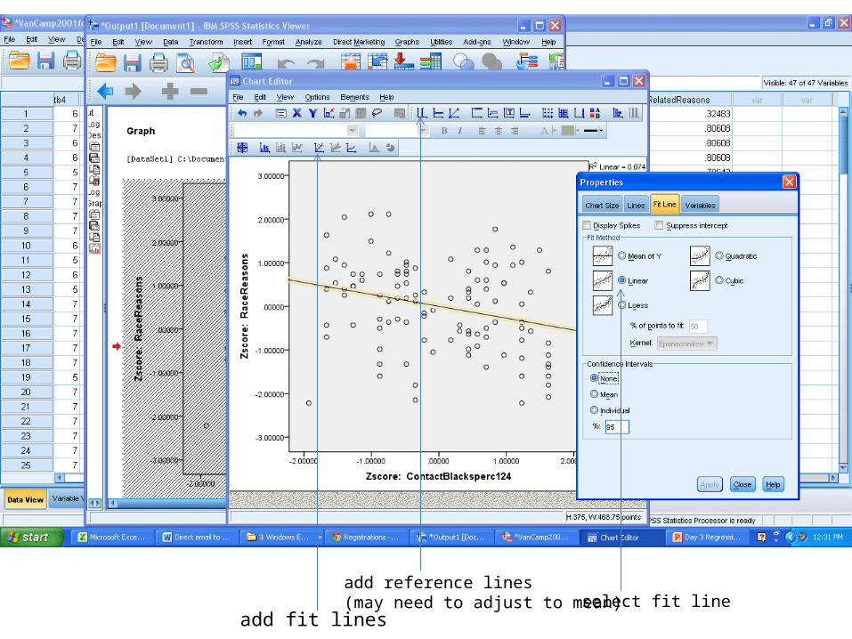
add fit lines
add reference lines(may need to adjust to mean) select fit line
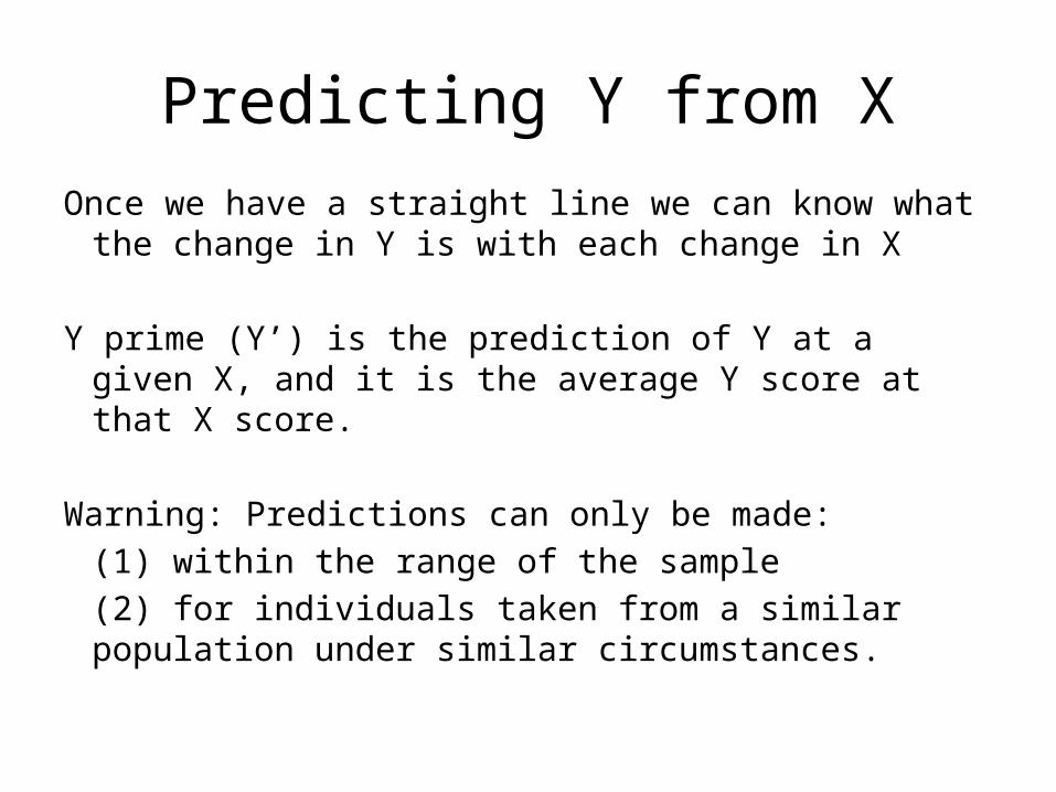
Predicting Y from X
Once we have a straight line we can know what the change in Y is with each change in X
Y prime (Y’) is the prediction of Y at a given X, and it is the average Y score at that X score.
Warning: Predictions can only be made:(1) within the range of the sample (2) for individuals taken from a similar population under similar circumstances.
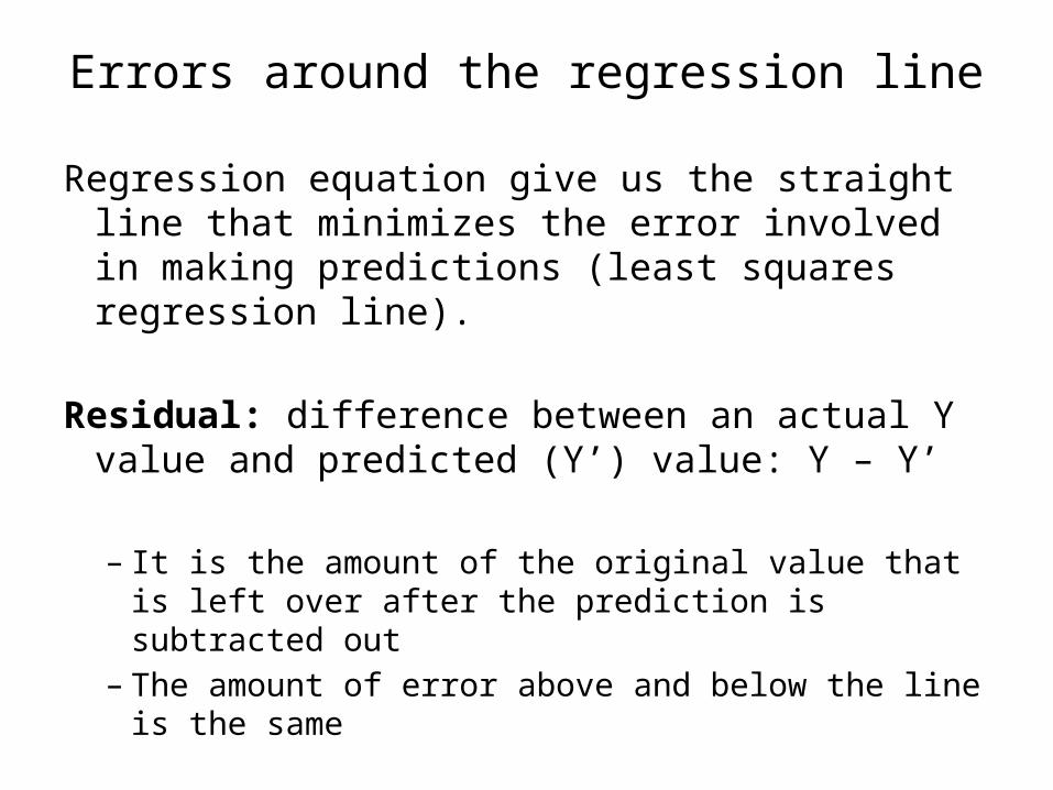
Errors around the regression line
Regression equation give us the straight line that minimizes the error involved in making predictions (least squares regression line).
Residual: difference between an actual Y value and predicted (Y’) value: Y – Y’
– It is the amount of the original value that is left over after the prediction is subtracted out
– The amount of error above and below the line is the same
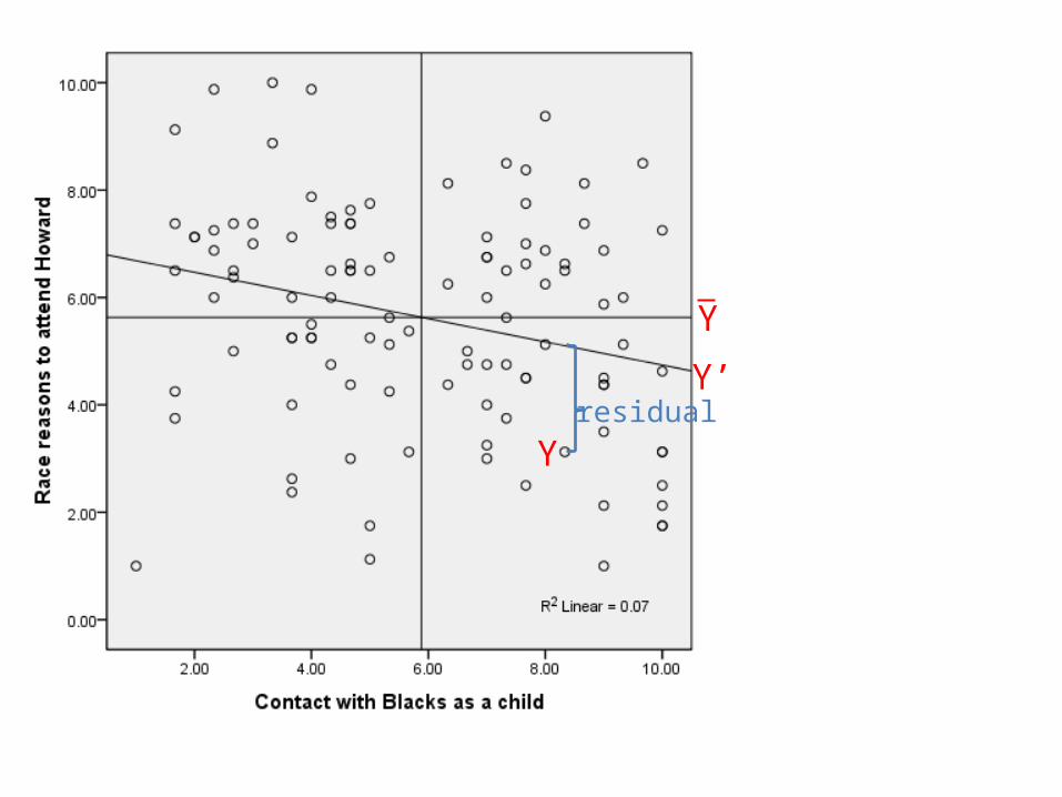
Y’
Y residual
Y
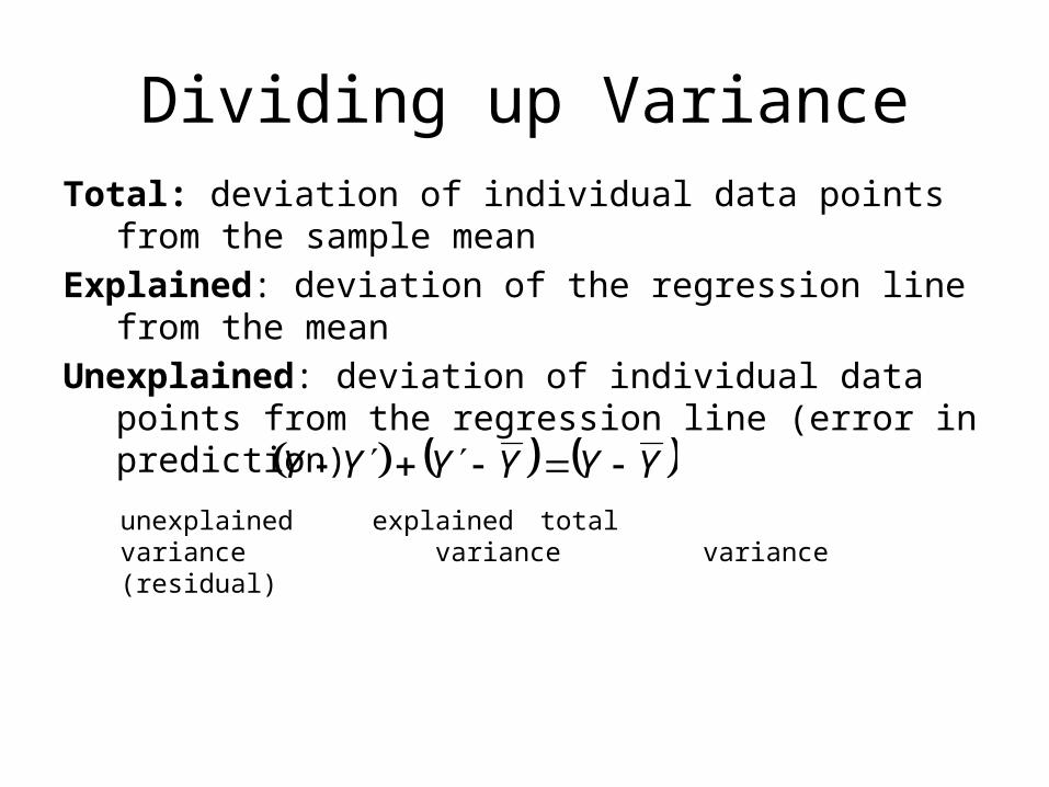
Dividing up VarianceTotal: deviation of individual data points from the sample meanExplained: deviation of the regression line from the meanUnexplained: deviation of individual data points from the
regression line (error in prediction)
YYYYYY unexplained explained total variance variance variance(residual)
Y
Y’
Y
residual
explainedtotal variance
YYYYYY unexplained explained total variancevariance variance(residual)
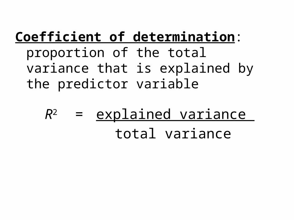
Coefficient of determination: proportion of the total variance that is explained by the predictor variable
R2 = explained variance total variance
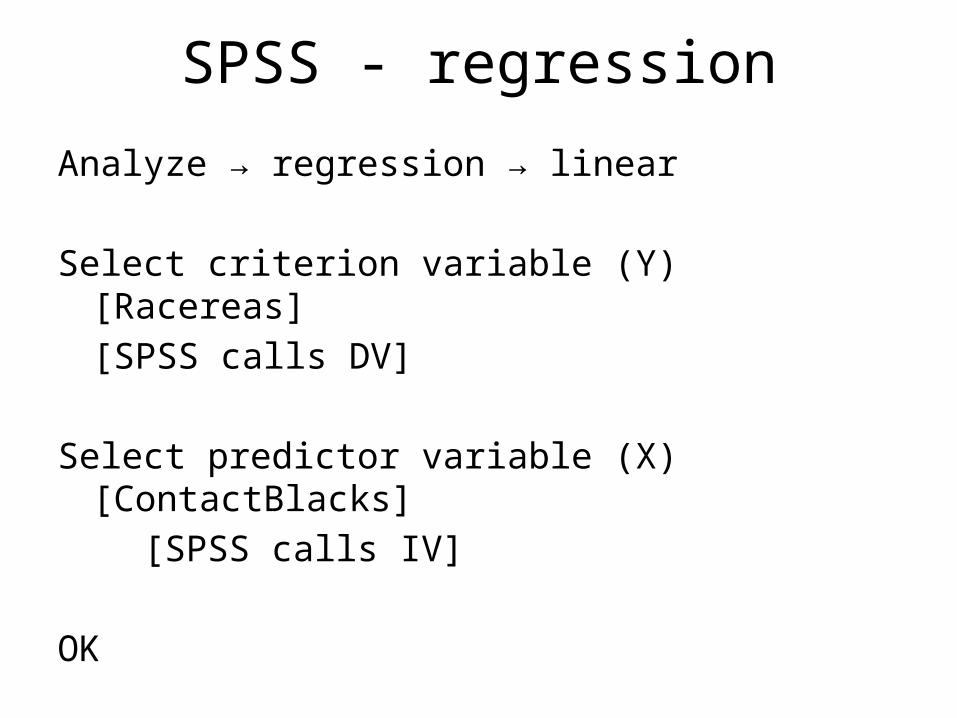
SPSS - regression
Analyze → regression → linear
Select criterion variable (Y) [Racereas][SPSS calls DV]
Select predictor variable (X) [ContactBlacks] [SPSS calls IV]
OK
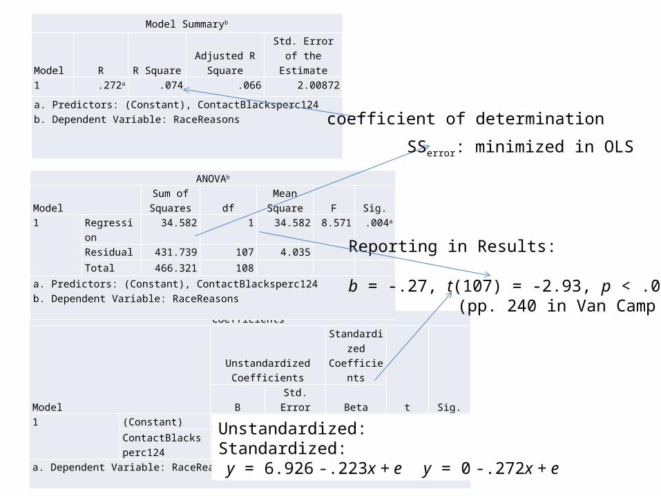
Coefficientsa
Model
Unstandardized Coefficients
Standardized Coefficients
t Sig.B Std. Error Beta1 (Constant) 6.926 .489 14.172 .000
ContactBlacksperc124
-.223 .076 -.272 -2.928 .004
a. Dependent Variable: RaceReasons
ANOVAb
ModelSum of Squares df
Mean Square F Sig.
1 Regression 34.582 1 34.582 8.571 .004a
Residual 431.739 107 4.035
Total 466.321 108
a. Predictors: (Constant), ContactBlacksperc124b. Dependent Variable: RaceReasons
Model Summaryb
Model R R SquareAdjusted R
SquareStd. Error of the
Estimate1 .272a .074 .066 2.00872
a. Predictors: (Constant), ContactBlacksperc124b. Dependent Variable: RaceReasons
Unstandardized: Standardized: y = 6.926 -.223x + e y = 0 -.272x + e
coefficient of determination
Reporting in Results:
b = -.27, t(107) = -2.93, p < .01. (pp. 240 in Van Camp 2010)
SSerror: minimized in OLS
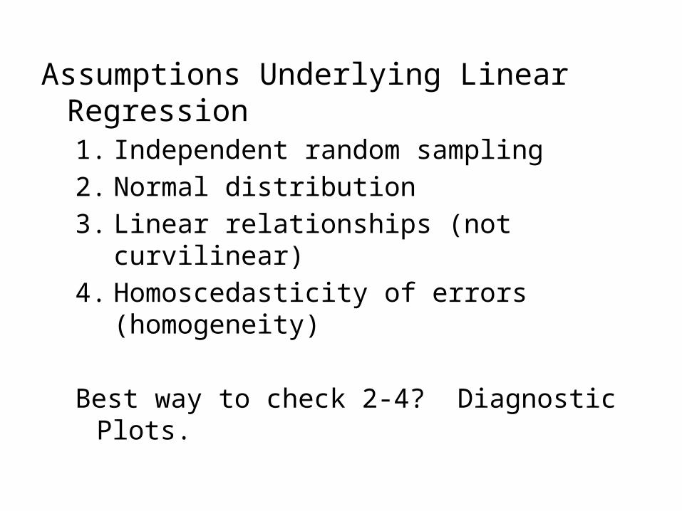
Assumptions Underlying Linear Regression1. Independent random sampling2. Normal distribution3. Linear relationships (not curvilinear) 4. Homoscedasticity of errors (homogeneity)
Best way to check 2-4? Diagnostic Plots.
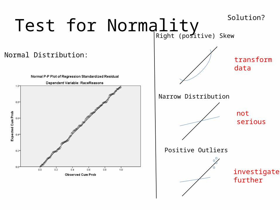
Test for NormalityRight (positive) Skew
Narrow Distribution
Positive Outliersooo
o
Normal Distribution:
Solution?
transformdata
notserious
investigatefurther
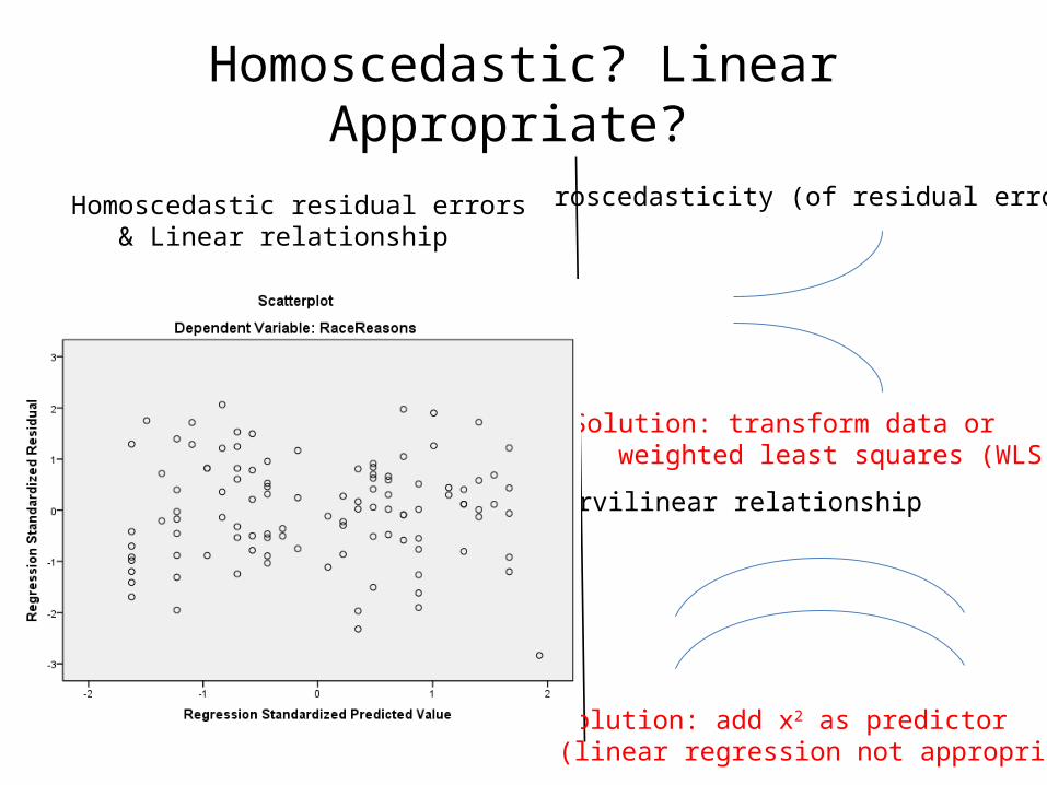
Homoscedastic? Linear Appropriate?
Heteroscedasticity (of residual errors)
Curvilinear relationship
Homoscedastic residual errors & Linear relationship
Solution: add x2 as predictor(linear regression not appropriate)
Solution: transform data or weighted least squares (WLS)
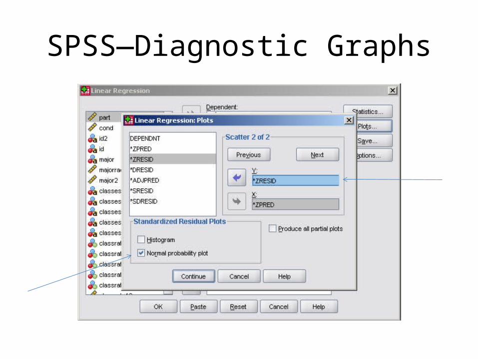
SPSS—Diagnostic Graphs

END


