Page 1
Simplified Trellis Decoding of Block Codesby Selective Pruning
Eric Bertrand
Department of Electrical & Computer EngineeringMcGill UniversityMontreal, Canada
February 2005
A thesis submitted to the Faculty of Graduate Studies and Research in partial fulfillmentof the requirements for the degree of Master of Engineering.
c© 2005 Eric Bertrand
Page 2
i
Abstract
Error correcting codes are of paramount importance for reliable communications. By adding
redundancy to the transmitted data they allow the decoder to detect and correct errors.
However in favorable channel conditions, a part of this redundancy can be removed in order
to increase throughput. Unfortunately most coding schemes are poorly adapted to these
higher coding rates. For example, the decoding of block codes grows exponentially with
code length. In this thesis we propose a novel solution to this problem: selective trellis
pruning.
Selective trellis pruning reduces decoding complexity by removing certain codewords
from the trellis. This reduction is accomplished by making hard decisions on the values
of bits in the received sequence above the certainty threshold. This method can produce
near-optimal results with only a fraction of the operation required by full decoding thanks
to the reduced trellis size. In this work we also introduce an innovative way of obtaining
the pruned trellis directly from a simplified version of the generator matrix. By using this
method we avoid the long process of constructing and then pruning the full trellises, thus
making the selective trellis pruning algorithm an efficient decoding tool. Finally we apply
this algorithm to the parallel concatenated turbo block code decoder in order to reduce its
complexity.
Page 3
ii
Sommaire
Les codes correcteurs d’erreur sont essentiels a une communication fiable. Ils rajoutent
une certaine quantite de redondance a l’information transmise afin que le decodeur puisse
detecter et corriger les erreurs de transmission. Cependant, lorsque les conditions de
transmission sont favorables, une partie de cette redondance peut etre enlevee afin de
d’augmenter la capacite du canal. Malheureusement, la majorite des techniques d’encodage
sont mal adaptees a ces taux d’encodage. Dans ces conditions, les codes convolutionels souf-
frent d’une perte de performance due au perforage tandis que la complexite du decodage des
codes en bloc augmente exponentiellement avec la longueur de ceux-ci. Dans ce memoire,
nous proposons une solution novatrice a ce probleme: la reduction selective du treillis.
La technique de reduction selective du treillis diminue la complexite de decodage des
codes en bloc en enlevant certains mots codes de leur treillis. Cette diminution est effectuee
en choisissant, avant le decodage, la valeur de tout les bits dans le signal recu au dessus
du seuil de simplification. En operant de cette facon il est possible d’atteindre un perfor-
mance quasi-optimale tout en n’utilisant qu’une infime partie des operation requises par
le decodage du treillis complet. Dans ce travail nous introduisons egalement une nouvelle
technique qui permet d’obtenir le treillis simplifie directement d’une version modifiee de la
matrice generatrice. De cette facon il est possible d’eviter le long processus de construction
et de reduction du treillis complet. En combinant ces deux techniques nous avons cree
un outil de decodage tres efficace. Finalement, nous avons applique ces principes a un
decodeur turbo utilisant de l’encodage en bloc parallele afin de reduire sa complexite.
Page 4
iii
Acknowledgments
First and foremost I thank my supervisor Fabrice Labeau for the support and guidance he
has provide over the course of this work. I also extend my deepest gratitude to my parents,
Linda and Jean-Claude, for their constant support throughout all my different endeavors.
I would also like to thank Caroline Rossi for her love, support and understanding during
the course of this work. I thank the National Science and Engineering Research Council of
Canada financial support over the past two years. Finally I would also like to acknowledge
the help of two friends: Fred Monfet for our fruitful discussions and Karim Ali for his lucid
insight.
Page 5
iv
Contents
1 Introduction 1
1.1 Thesis Contribution . . . . . . . . . . . . . . . . . . . . . . . . . . . . . . . 2
1.2 Thesis Organization . . . . . . . . . . . . . . . . . . . . . . . . . . . . . . . 3
2 Background 5
2.1 Linear Block Codes . . . . . . . . . . . . . . . . . . . . . . . . . . . . . . . 5
2.2 Trellis Representation of Block Codes . . . . . . . . . . . . . . . . . . . . . 7
2.2.1 Trellises . . . . . . . . . . . . . . . . . . . . . . . . . . . . . . . . . 7
2.2.2 Trellis representation of Block Codes and Trellis Construction . . . 8
2.3 Viterbi Decoding . . . . . . . . . . . . . . . . . . . . . . . . . . . . . . . . 14
2.3.1 Hard Input, Hard Output . . . . . . . . . . . . . . . . . . . . . . . 15
2.3.2 Soft Input, Hard Output . . . . . . . . . . . . . . . . . . . . . . . . 16
2.3.3 SOVA or Soft Input, Soft Output . . . . . . . . . . . . . . . . . . . 16
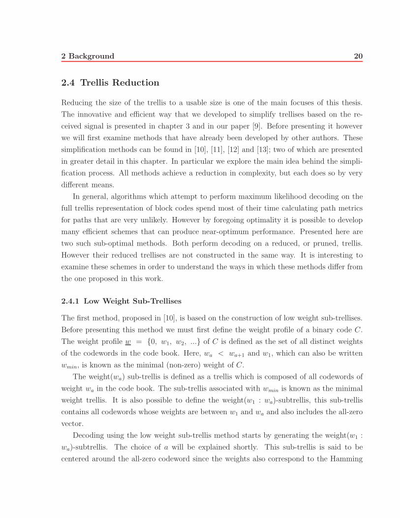
2.4 Trellis Reduction . . . . . . . . . . . . . . . . . . . . . . . . . . . . . . . . 20
2.4.1 Low Weight Sub-Trellises . . . . . . . . . . . . . . . . . . . . . . . . 20
2.4.2 Chase Decoding . . . . . . . . . . . . . . . . . . . . . . . . . . . . . 21
2.5 Turbo Codes . . . . . . . . . . . . . . . . . . . . . . . . . . . . . . . . . . . 21
2.5.1 Serial Concatenated Block Codes . . . . . . . . . . . . . . . . . . . 22
2.5.2 Parallel Concatenated Block Codes . . . . . . . . . . . . . . . . . . 22
2.5.3 Product Codes . . . . . . . . . . . . . . . . . . . . . . . . . . . . . 23
2.5.4 Turbo Decoding . . . . . . . . . . . . . . . . . . . . . . . . . . . . . 25
3 Selective Trellis Pruning 28
3.1 Selective Trellis Pruning . . . . . . . . . . . . . . . . . . . . . . . . . . . . 29
3.1.1 Bit Selection . . . . . . . . . . . . . . . . . . . . . . . . . . . . . . . 29
Page 6
Contents v
3.1.2 Simplification Order . . . . . . . . . . . . . . . . . . . . . . . . . . 31
3.1.3 Amount of simplification . . . . . . . . . . . . . . . . . . . . . . . . 33
3.1.4 Implementation Issues . . . . . . . . . . . . . . . . . . . . . . . . . 36
3.1.5 Trellis Pruning via Generator Matrix Simplification . . . . . . . . . 37
3.2 Trellis Pruning as Applied to a Turbo Decoder . . . . . . . . . . . . . . . . 41
4 Experimental Results 44
4.1 Systematic vs. Redundant Bit Simplification . . . . . . . . . . . . . . . . . 44
4.2 Trellis Reduction Using Selective Trellis Pruning . . . . . . . . . . . . . . . 47
4.2.1 Test Setup . . . . . . . . . . . . . . . . . . . . . . . . . . . . . . . . 47
4.2.2 Results . . . . . . . . . . . . . . . . . . . . . . . . . . . . . . . . . . 49
4.2.3 Behavior . . . . . . . . . . . . . . . . . . . . . . . . . . . . . . . . . 53
4.2.4 Simplifications and Appropriate Thresholds . . . . . . . . . . . . . 54
4.3 Turbo Decoding . . . . . . . . . . . . . . . . . . . . . . . . . . . . . . . . . 57
4.3.1 Test Setup . . . . . . . . . . . . . . . . . . . . . . . . . . . . . . . . 57
4.3.2 Results . . . . . . . . . . . . . . . . . . . . . . . . . . . . . . . . . . 58
4.3.3 Behavior . . . . . . . . . . . . . . . . . . . . . . . . . . . . . . . . . 61
4.3.4 Savings . . . . . . . . . . . . . . . . . . . . . . . . . . . . . . . . . 62
5 Conclusion 63
5.1 Summary . . . . . . . . . . . . . . . . . . . . . . . . . . . . . . . . . . . . 63
5.2 Future Work . . . . . . . . . . . . . . . . . . . . . . . . . . . . . . . . . . . 65
5.2.1 Dynamic Threshold Updating . . . . . . . . . . . . . . . . . . . . . 65
5.2.2 Best k Bit Simplification Method . . . . . . . . . . . . . . . . . . . 65
5.2.3 Additional Turbo Simplifications . . . . . . . . . . . . . . . . . . . 66
A Generator Matrices 67
References 71
Page 7
vi
List of Figures
2.1 Trellis representation of the (7,3) block code using 56 edges and 50 states. . 9
2.2 Trellis representation of the (7,3) block code using 28 edges and 22 states. . 10
2.3 Trellis representation of the (7,3) block code using 22 edges and 18 states. . 10
2.4 Pseudo Code for the Viterbi Algorithm. . . . . . . . . . . . . . . . . . . . . 15
2.5 Pseudo Code for the SOVA Algorithm. . . . . . . . . . . . . . . . . . . . . 19
2.6 Serial Concatenated Block Code Encoder . . . . . . . . . . . . . . . . . . . 22
2.7 Parallel Concatenated Block Code Encoder . . . . . . . . . . . . . . . . . . 23
2.8 Serial Concatenated Product Code Encoder. . . . . . . . . . . . . . . . . 24
2.9 Parallel Concatenated Product Block Code Encoder. . . . . . . . . . . . . 24
2.10 Parallel Iterative Turbo Decoder . . . . . . . . . . . . . . . . . . . . . . . . 25
3.1 Pseudo Code of the selective trellis pruning algorithm . . . . . . . . . . . . 35
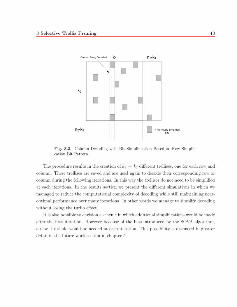
3.2 Row Decoding with Bit Simplification. . . . . . . . . . . . . . . . . . . . . 42
3.3 Column Decoding with Bit Simplification Based on Row Simplification Bit
Pattern. . . . . . . . . . . . . . . . . . . . . . . . . . . . . . . . . . . . . . 43
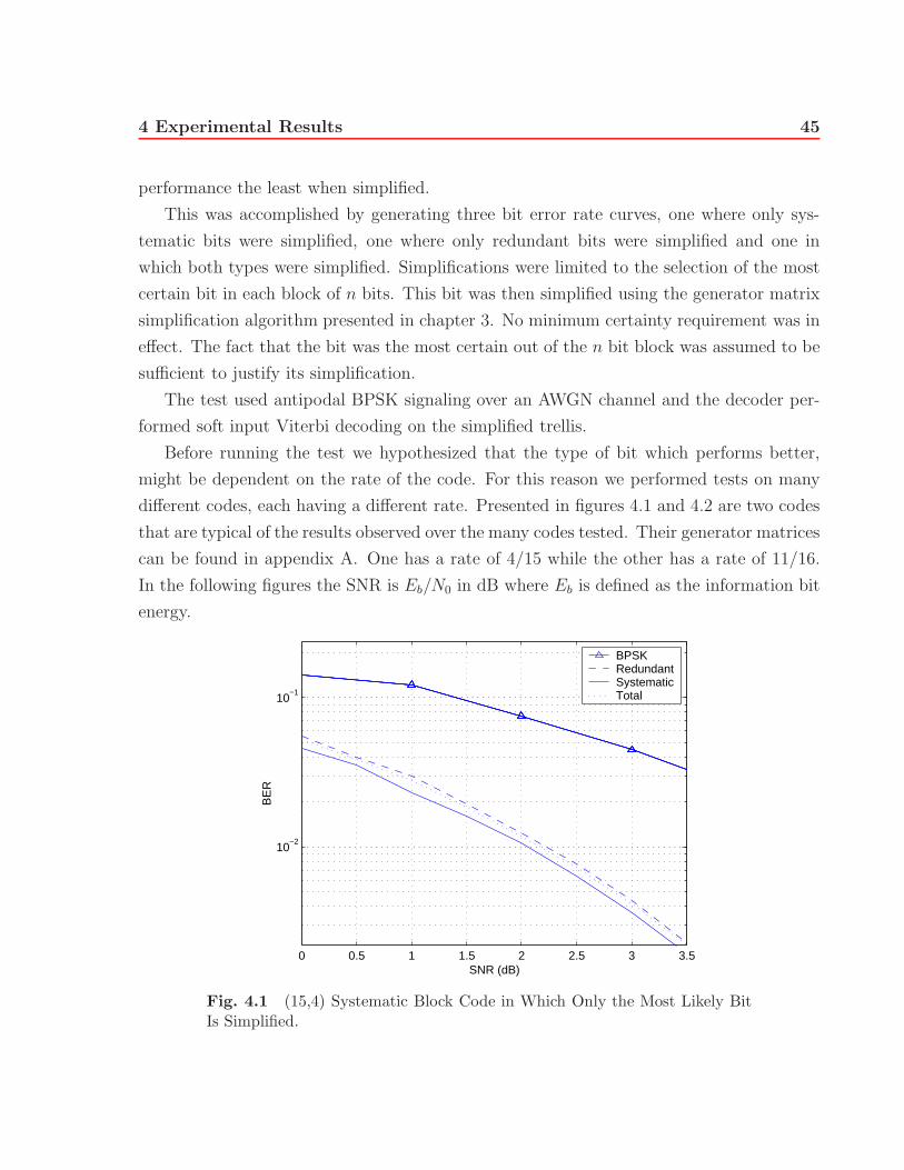
4.1 (15,4) Systematic Block Code in Which Only the Most Likely Bit Is Simplified. 45
4.2 (16,11) Systematic Block Code in Which Only the Most Likely Bit Is Simplified. 46
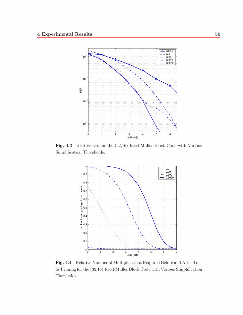
4.3 BER curves for the (32,16) Reed-Muller Block Code with Various Simplifi-
cation Thresholds. . . . . . . . . . . . . . . . . . . . . . . . . . . . . . . . 50
4.4 Relative Number of Multiplications Required Before and After Trellis Prun-
ing for the (32,16) Reed-Muller Block Code with Various Simplification
Thresholds. . . . . . . . . . . . . . . . . . . . . . . . . . . . . . . . . . . . 50
4.5 BER curves for the (31,16) BCH Block Code with Various Simplification
Thresholds. . . . . . . . . . . . . . . . . . . . . . . . . . . . . . . . . . . . 51
Page 8
List of Figures vii
4.6 Relative Number of Multiplications Required Before and After Trellis Prun-
ing for the (31,16) BCH Block Code with Various Simplification Thresholds. 51
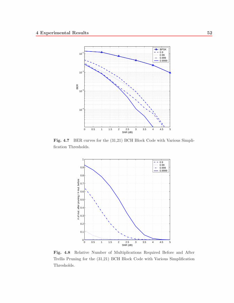
4.7 BER curves for the (31,21) BCH Block Code with Various Simplification
Thresholds. . . . . . . . . . . . . . . . . . . . . . . . . . . . . . . . . . . . 52
4.8 Relative Number of Multiplications Required Before and After Trellis Prun-
ing for the (31,21) BCH Block Code with Various Simplification Thresholds. 52
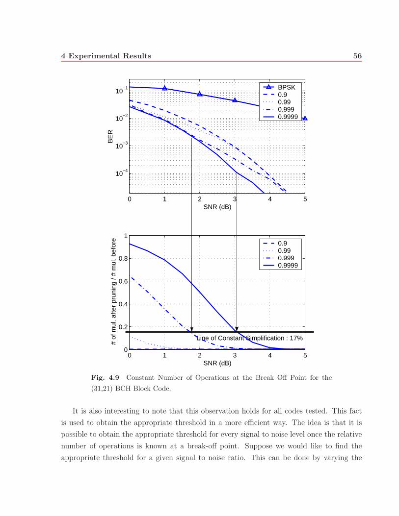
4.9 Constant Number of Operations at the Break Off Point for the (31,21) BCH
Block Code. . . . . . . . . . . . . . . . . . . . . . . . . . . . . . . . . . . . 56
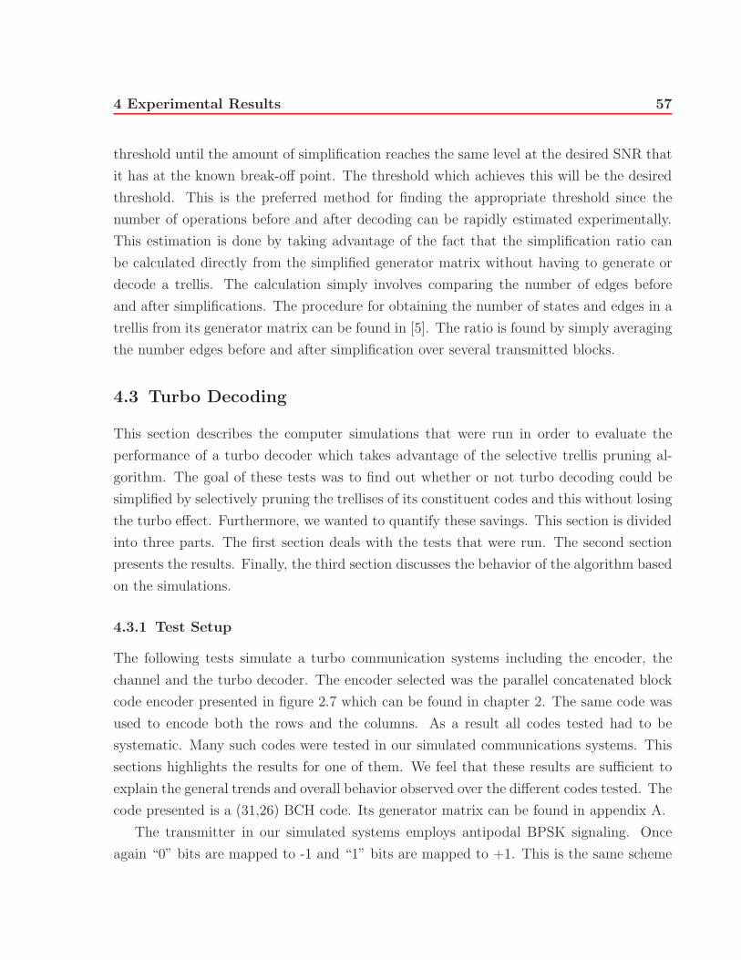
4.10 Bit Error Rate Curves for the First 3 Iterations of Turbo Decoding Using
No Simplifications for the (31,26) BCH Block Code. . . . . . . . . . . . . . 59
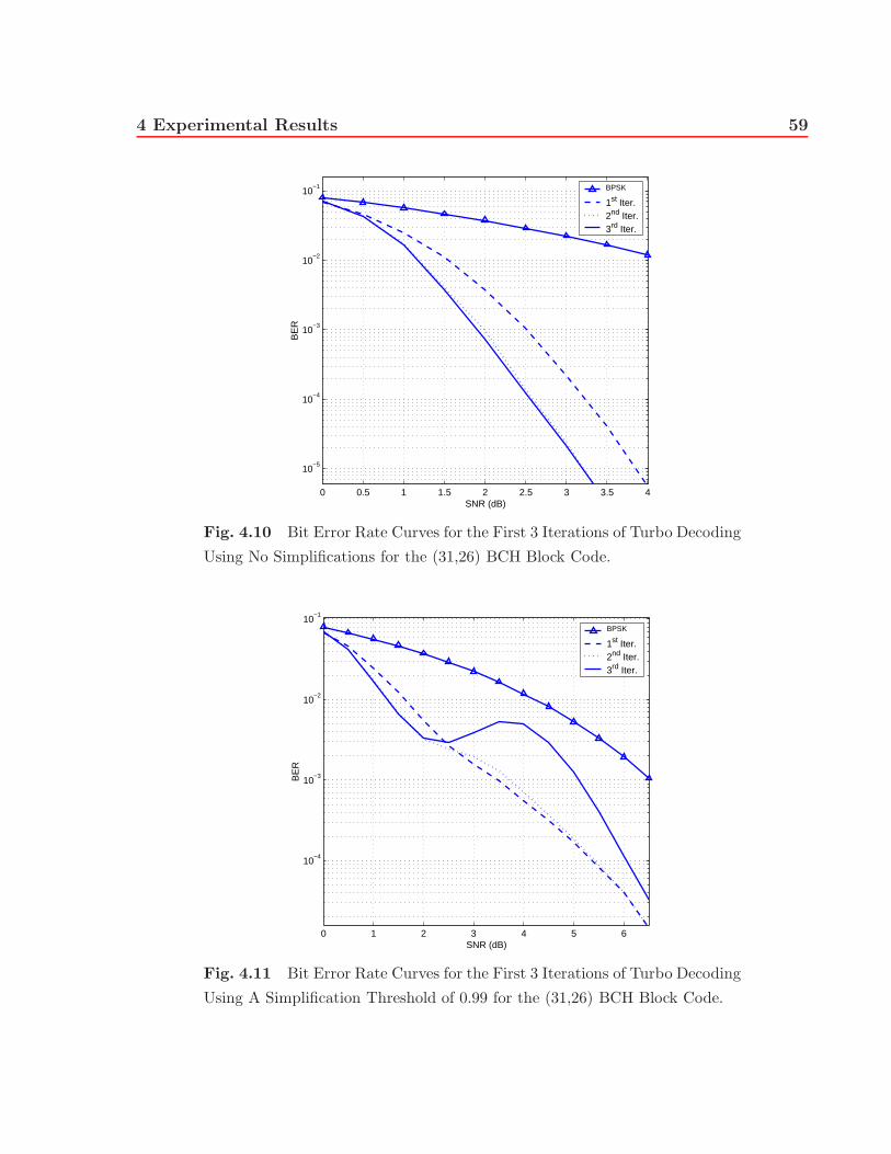
4.11 Bit Error Rate Curves for the First 3 Iterations of Turbo Decoding Using A
Simplification Threshold of 0.99 for the (31,26) BCH Block Code. . . . . . 59
4.12 Bit Error Rate Curves for the First 3 Iterations of Turbo Decoding Using A
Simplification Threshold of 0.999 for the (31,26) BCH Block Code. . . . . . 60
4.13 Relative Number of Multiplications Required Before and After Trellis Prun-
ing for the Turbo Decoder of the (31,21) BCH Block Code with Various
Simplification Thresholds. . . . . . . . . . . . . . . . . . . . . . . . . . . . 60
Page 9
1
Chapter 1
Introduction
Digital communications have become part of our everyday life. From the internet, to
cell phones, to satellite television, our society now relies heavily on this technology. New
applications are constantly popping up and the number of people using these systems
increases daily. This increase in demand has lead designers to develop communication
systems that are incredibly efficient and reliable. However, new applications are now being
developed which will require systems to be even more efficient then in the past. Third
generation, or 3G cell phones push the envelope by proposing mobile video conferencing
and mobile high speed internet. Home internet speeds have increased more then ten-fold
in the past years. All this leads to an increased demand on data transmission. As more
and more data is sent over these networks it is important that they remain reliable.
Error-correcting codes play a key role in these systems, be they wireline or wireless.
For unidirectional systems, they add a certain amount of redundancy to the data that en-
ables the receivers to detect and correct errors. For bidirectional communication systems
this redundancy limits the number of retransmissions needed to ensure reliable commu-
nication. This increases throughput not only by minimizing retransmissions but also by
allowing transmitters to use more efficient modulation schemes. These schemes pack more
bits/second per Hertz and could not be used on some channels due to error rate consid-
erations. In case of extremely poor conditions, error correcting codes allow systems to
communicate on channels that would otherwise be unusable.
On the other hand when channel conditions are favorable, the amount of redundancy
introduced can be reduced in order to augment throughput. At these rates however conven-
Page 10
1 Introduction 2
tional error correcting schemes are not at their best. This is because the implementation
of error correcting systems using convolution codes become very complex and their perfor-
mance can sometimes suffer due to the use of puncturing. Systems using block codes can
easily be designed for these higher rates but the computational complexity of the trellis
decoding algorithm is prohibitive. In order to solve this problem we investigated different
ways of reducing the computational complexity of decoding block codes.
The source of the complexity required by the decoding algorithm was identified as the
extremely large trellis representation of block codes. The idea behind the methods we
developed was to reduce the size of this trellis representation while still maintaining near-
optimal performance. In other words our method trades optimality in order to reduce
decoding complexity.
From a throughput point of view turbo codes could also benefit from a reduction in the
amount of redundancy added to the data when channel conditions are favorable. For this
reason we also investigated applying one of our trellis simplification methods to the decoder
of a parallel concatenated turbo block code encoder. More specifically the algorithm is used
to simplify the decoding of the different constituent codes. This work presents our research
into these computationally efficient decoding algorithms.
1.1 Thesis Contribution
This thesis proposes a new algorithm which can select a certain number of codewords, based
on the received signal, which, when removed from the trellis representation of a block code,
do not affect performance significantly. These codewords do, on the other hand, reduce
the number of operations required by the decoder to a fraction of those required by full
decoding. This algorithm is referred to as the selective trellis pruning algorithm.
An innovative algorithm for removing these codewords from the trellis is also proposed.
This algorithm is capable of modifying the generator matrix of the code so that it generates
only the codewords in the pruned trellis. In this way the simplified trellis can be generated
directly instead of having to generate a complete trellis and then reduce it.
This thesis also introduces a turbo decoding scheme with reduced complexity. This
scheme incorporates our innovative selective trellis pruning algorithm inside the soft output
Viterbi decoders of the constituent codes.
Page 11
1 Introduction 3
1.2 Thesis Organization
Chapter 2 discusses a variety of subjects related to error correcting codes. More specifically
it deals with various coding techniques and the trellis representations of block codes. The
coding technique presented include linear block codes in their general form. The concepts
of the generator and parity check matrices are defined and the way in which block codes
are used in error detection and correction is explored. Turbo coding is also presented with
various encoders and decoders. In particular product codes are discussed. This is also
where the Viterbi algorithm is presented in its different forms. The coding techniques
are followed by a discussion on the different ways a block code can be represented by a
trellis. In particular we focus on the selection of the optimal representation. Two methods
proposed in previous work for reducing the trellis to a usable size are also presented. These
methods are the low-weight sub-trellis method and the Chase method. This chapter also
introduce the notations that will be used throughout this thesis.
The third chapter focuses on the novel contributions proposed in this work. The design
of the selective pruning algorithm is discussed in detail. This includes the selection of the
bits to be simplified, the selection of the simplification order as well as the introduction
of the simplification threshold. It also explores different implementation issues regarding
this algorithm. The innovative way in which we obtain the pruned trellis directly from a
simplified version of the generator matrix and a translation vector is derived. This method
results in significant computational savings during the selective trellis pruning algorithm.
We also propose a novel way of using our pruning algorithm to reduce the complexity of a
turbo decoder. This algorithm simplifies bits in the received signal, before the first iteration
of decoding is performed, in the same way as it would in a non-turbo setting.
In chapter four we present the experimental results obtained for the different tests run
during the course of this work. These tests are divided into three main parts. The first part
presents the tests used to determine which bits should be simplified by our algorithm. They
determine whether it is better to simplify systematic or redundant bits. This is followed by
the tests that were run in order to analyze the behavior of the selective pruning algorithm
under different operating conditions. In particular it examines how certain block code char-
acteristics affect performance as well as the amount of savings that can be achieved when
using our algorithm. This is also where we develop a method for finding an appropriate
simplification threshold based on a code and signal to noise ratio. Finally, the results of
Page 12
1 Introduction 4
tests run on the turbo decoder using trellis simplifications are presented. Again our focus
is on algorithm behavior and the amount of simplifications that can be achieved.
While developing these algorithms new ideas often occurred to us. Some of these were
related to improvements that could be made to the algorithms developed while others were
new ideas based on similar principles that we believe could be exploited. However these
ideas are beyond the scope of this work and for this reason are presented in chapter 5.
Page 13
5
Chapter 2
Background
2.1 Linear Block Codes
Error correcting codes are of paramount importance to reliable communications. These
codes add a certain amount of redundancy to the data which can be used to detect and/or
correct errors that occur during transmission. Forward error correcting codes (FEC) are
used in one-way communication systems. When errors are detected these systems cannot
send a request for retransmission to the transmitter, thus it is up to the receiver to correct
the errors with the information present in the received signal. Linear block codes are just
one of many types of codes that can be used to accomplish this. In this section we will
mathematically describe them as well as present many related concepts.
A linear block code is defined by a set of codewords known as the code book [1]. Each
codeword is a vector which contains exactly n symbols. The symbols can be chosen for
an alphabet containing any number of elements. However when the alphabet has only two
elements we say that the code is binary and each symbol is known as a bit. This is the case
for all codes used in this work and for this reason all definitions and proofs will suppose
that the codes in question are binary.
Given n bits 2n, different possible combinations can be created. We define the code
book of a block code by choosing a subset of say 2k combinations, or code words, out of
2n possibilities. In this fashion 2k k-tuples are mapped into 2k n-tuples and we say the
we have an (n, k) code. If a k × n generator matrix G is used to map the k-tuples to the
n-tuples the resulting code is known as (n, k) linear block code.
Mathematically, given a k-bit message u = (u1, u2, ..., uk) we introduce n − k bits of
Page 14
2 Background 6
redundancy using a k-by-n generator matrix G in order to obtain an n bit codeword
c = (c1, c2, ..., cn). This is accomplished as follows :
c = uG (2.1)
It should be noted that since the elements of the vectors and of the matrices are all
binary the operations of addition and multiplication are carried out in GF(2). Related to
the generator matrix is the parity check matrix H. This matrix is the generator matrix
for the dual code associated to the linear code defined by G. The dual code is made up of
the 2n−k code words that constitute the null space of G. This implies that any code word
generated by G is orthogonal to all code words in the dual code and hence:
cH′ = 0 (2.2)
Using Eq. (2.1) we can see that:
uGH′ = 0 ⇒ GH′ = 0 (2.3)
The fact that all codewords are orthogonal to their parity check matrix is often used in
error detection. If the result of the multiplication between the received signal and the parity
check matrix is not 0 then the received sequence is not a codeword and a transmission error
has occurred. Error correction using block codes is achieved by selecting the n-tuple, out
of the 2k valid n-tuples, which is closest to the noisy observation of c.
In order to compare different block codes we will now define several concepts that
characterize them. First, the rate of a block code is defined as the ratio k/n. This represents
the amount of redundancy added by the code. The lower the rate, the more redundancy is
present. A ratio of 1 means no redundancy is present and is equivalent to an interleaver.
Unlike some types of error correcting codes, block codes can easily be designed with high
or low coding rates.
Another important characteristic of a linear block code is whether or not it is systematic.
In a systematic code the k-bit message can be seen directly in the n-bit codeword. In other
words for a systematic code it is possible to re-write the generator matrix in the following
form :
G =[
Ik×k Pk×(n−k)
](2.4)
Page 15
2 Background 7
simply by reordering the columns of G. Here Ik×k is the identity matrix and Pk×(n−k) is
the matrix responsible for the parity bits. For the case of non-systematic codes, obtaining
the message bits from the coded bits is more involved since each code bit is part message
and part redundancy.
The weight of a codeword denoted w(c) is equal to the number of non-zero entries in
the codeword. For example:
w(1 0 1 0 0 1) = 3 (2.5)
Finally block codes can also be characterized by their minimum distance, denoted by
dmin. It is not uncommon to refer to a code as a (n, k, dmin) code. This distance is defined
as the the smallest Hamming distance between two codewords in the code book. The
Hamming distance between two codewords is simply equal to the number of bit positions
in which the two differ. The minimum distance is closely related to the error correcting
capability of a code. The greater the minimum distance the better since the valid code
words are farther apart.
2.2 Trellis Representation of Block Codes
Trellises are often used in the decoding process in order to keep track of all valid codewords
and compare them to the received signal. Coupled with efficient decoding algorithms such
as Viterbi and BCJR, they can be powerful tools. In this section we first define trellises
in general terms, while introducing the notation that will be used throughout this work.
This is followed by the detailed presentation of the trellis representation of block codes.
And finally we examine the process of trellis generation. For full details on the trellis
representation of block codes we refer the reader to [2].
2.2.1 Trellises
Mathematically a trellis T is a layered directed graph. It is defined by three different sets.
They are, a set of states V , a set of edges E and a set of labels λ. States are grouped
together to form depths. In figures 2.1, 2.2, 2.3 the states are represented by numbers.
These states are numbered from 0 at each depth. Edges in the trellis are responsible for
linking states at different depths. They are represented by arrows in the trellis figures.
Page 16
2 Background 8
Finally, each label is associated to a specific edge and contains information related to that
edge. In the figures, the labels are represented by solid and dashed lines. A solid line
represents a binary value of 0 in the corresponding code word at the appropriate position
while a dashed line represents a 1.
Specifically, the layers of the trellis are organized by depth and are indexed by x ∈[0, 1, 2, ..., n] where n, known as the length of the code, is defined as the greatest depth in
the trellis.
We denote the set of all states in all depths by V and the set of all states at depth given
depth x by Vx. The number of states at each depth depends on the code which is being
represented.
E is defined as the set of all edges in the trellis and Ex,x+1 are subsets of E and contain
all edges linking a state in Vx to a state in Vx+1. Each state in the trellis must have at least
one edge entering it and one edge leaving it unless the state is on the limits of the graph
(i.e. x = 0 or x = n). Edges must not jump over a depth. In other words an edge cannot
connect a state in Vx to one in Vx+a where a is any integer greater than 1. Each edge in E
also has an associated label λe in λ.
The two operators start() and end() return the start and end states of a given edge.
For example given and edge e that links state v1 to state v2, start(e) is v1 and end(e) is v2.
A path is defined as a set of uninterrupted edges which links two states in a trellis.
Let v1 and v2 be two states in V where v1 ∈ Va and v2 ∈ Vb and a < b. We define a
path Pv1,v2 as a set of edges (e1, ..., eb−a) for which start(e1) = v1, end(eb−a) = v2 and
end(ex) = start(ex+1) where x ∈ 1, ..., b−a−1. It is possible that more than one path link
two given states and the set of all such paths is denoted by Φv1,v2.
Finally the label of a path denoted λ(P ) is equal to the concatenation of the labels of
the edges in P , i.e. λ(P ) = (λe1λe2 ...λeb−a).
2.2.2 Trellis representation of Block Codes and Trellis Construction
We say that a trellis T (V, E, λ) represents a block code C if and only if λ(ΦσI ,σF) is identical
to the codewords of C. In other words only when the labels of each and every path from
σI to σF corresponds to a codeword in C and that all codewords in C have a corresponding
path in T can we say that T represents C.
This definition leads to many possible trellis representations of a given code. That is to
Page 17
2 Background 9
say the trellis representation of a block code is not unique. To illustrate this point we will
examine three different representations for the (7,3) code defined by:
G =
1 0 1 0 0 1 1
1 0 1 0 1 0 0
1 1 1 1 0 0 0
(2.6)
We can see from the generator matrix that this code is systematic. Figures 2.1, 2.2, 2.3
show three possible trellis representations for this code.
0 ��
������
���
�����
����
����
���
�����
����
����
����
����
��
��
��
��
��
0 �� 0 �� 0 �� 0 �� 0 �� 0 �� 0
1 �� 1 �� 1 �� 1 �� 1 �� 1
��
2 �� 2 �� 2 �� 2 �� 2 �� 2
����������������
3 �� 3 �� 3 �� 3 �� 3 �� 3
4 �� 4 �� 4 �� 4 �� 4 �� 4
�����������������������������
5 �� 5 �� 5 �� 5 �� 5 �� 5
��
6 �� 6 �� 6 �� 6 �� 6 �� 6
����������������������������������������������
7 �� 7 �� 7 �� 7 �� 7 �� 7
��
Fig. 2.1 Trellis representation of the (7,3) block code using 56 edges and 50states.
Since many different trellises can represent a given block code a choice must be made
as to which representation should be selected. The first representation 2.1 is the most
straightforward and can be easily constructed directly from the code book. This is done by
simply adding n − 1 states and n edges for each codeword in the code book to the trellis
presenting the all-zero codeword in such a way that each path from start to finish represents
Page 18
2 Background 10
0 ��
������
���
��
��
0 �� 0 �� 0 �� 0 �� 0 �� 0 �� 0
1 �� 1 �� 1 �� 1 �� 1 �� 1
��
2 �� 2 �� 2 �� 2
���������
��
3 �� 3 �� 3 �� 3
����������������
Fig. 2.2 Trellis representation of the (7,3) block code using 28 edges and 22states.
0 ��
��
0 ��
��
0 �� 0 �� 0 ��
��
0 �� 0 �� 0
1
�����
����
����
���
��
1 �� 1
��
1 ��
��
1 �� 1
��
2 �� 2
��
3 �� 3
����������������
Fig. 2.3 Trellis representation of the (7,3) block code using 22 edges and 18states.
Page 19
2 Background 11
one of the codewords. However, as we will present shortly, the decoding complexity of the
Viterbi algorithm is directly related to the number of edges and states in the trellis. Seeing
as the ultimate goal of our algorithm is to simplify decoding we would obviously like to select
the representation with the smallest decoding complexity and hence the smallest number
of edges and states. With this in mind, we note that despite the fact that the trellis in 2.1
is easy to construct, it uses the greatest number of states and edges. Specifically the trellis
contains 8 paths, since there are 23 = 8 codewords, each requiring 7 edges, since n = 7.
8 paths ∗ 7 edges
path= 56 edges (2.7)
This means that a total of 56 edges and 50 states are required to represent the code
using this trellis representation. The graphs in in figures 2.2 and 2.3 take advantage of the
fact it is possible to share certain states and edges between different paths. This sharing
reduces the number edges required to 28 and the number of states to 22 in figure 2.3. The
third representation (figure 2.3) does even better, using only 22 edges and 18 states to
represent the entire code book.
We say that a trellis is in minimal form when it uses no more edges or states than is
strictly necessary. In other words a trellis with fewer states or edges could not represent
all codewords in the code book. It can be shown that for each code there exist such a
representation [3]. A full discussion on the dimension of the trellis representation of block
codes can be found in [4]. This minimal trellis is the desired representation and will be
used throughout the rest of this work.
We now focus on the construction of this minimal trellis. There are many algorithms for
finding the minimal trellis of a block code directly from its generator matrix. The approach
that we use can be found in [5]. The process is quite involved but is computationally
efficient. Re-deriving this algorithm in its entirety would be overly complicated and would
not provide the reader with additional insight into our selective pruning algorithm. This
is because the trellis construction algorithm is only used to provide the simplest trellis
representation given a generator matrix. In other words it provides a starting point for our
simplifications. For these reason we only present the main idea behind this algorithm.
The first step in constructing the minimal trellis is to put the generator matrix into its
minimal-span form. In order to define this form is we introduce several other definitions.
First, the span of a non-zero vector x is the discrete interval or indices between the smallest
Page 20
2 Background 12
index (Left(x)) such that xi �= 0 and the largest index (Right(x)) such xi �= 0. The span
length of x denoted spanlenght(x) is equal to the number of elements in the span. The span
length of a matrix is then defined as the sum of the span length of it rows. Finally a matrix
is in minimal-span form when its span length is as small as possible and is row-equivalent to
the original matrix. Full details on two algorithms for obtaining the minimal span matrix
can be found in [5]. Minimal span matrices are part of a useful class of generator matrices
for linear codes said to be ‘’trellis oriented”. In this form many useful properties can be
read directly from generator matrix.
We now define some of these properties. First we say that a vector x is active at
coordinate i if i is in the span of x. Second we say that a vector is active at depth i if both
i and i + 1 are in the span of x. It is clear that it is possible to determine if a row in a
matrix is active at coordinate i or at depth i directly. Using these concepts we now define
two set Ai and Bi. Ai is defined as the set of row indices which are active at coordinate i
in matrix. Similarly Bi is defined as the set of row indices which are active at depth i in
the matrix. Finally αi and βi are the cardinalities of Ai and Bi respectively. For example
if a generator matrix G is active at coordinate i = 3 in rows 2 and 3 then A3 = {2, 3} and
α3 = 2.
We can now proceed with construction of the trellis. This is done in two steps. First
the states are added and then they are linked together. The number of states allocated
at depth i is 2βi since |Vi| = 2βi [5]. The number of edges required to link these states
is 2αi. The linking procedure uses Ai, Bi, αi and βi in order to determine how to link
the different states together as well as assign their corresponding label. This procedure is
fairly straight forward but quite lengthy. For this reason we refer the reader to [5] for full
details. However it is clear that all four of these values can be obtained directly from the
generator matrix. The trellis that is generated is minimal when the generator matrix is in
its minimal-span form. In this way it is possible to obtain the desired minimal trellis from
any generator matrix.
The trellis representation is well known when it comes to convolutional codes. There
are however several differences between these trellises and those that represent block codes.
First the trellises used for decoding convolutional codes normally have an undefined length.
For this reason only a certain number of past depths are considered during the decoding
process. On the other hand the depth in the case of block code is well defined and is equal
to n. Bits are output during the decoding process only after the entire trellis has been
Page 21
2 Background 13
searched.
It is also typical for the trellis of convolutional codes to have the same structure at
each depth of the trellis and they do not tend to be very wide. This regularity can be
used to simplify the implementation of the decoding algorithm. On the other hand, block
codes have a trellis structures that can vary greatly from depth to depth. In other words
some depth can have a great many states while others can have very few. This means that
the decoding complexity of the different depths varies from depth to depth and requires a
decoding algorithm capable of dealing with this situation. This variation is obvious when
one considers the fact that all codewords in a block code start and end in the same states,
these states are known as the initial (σi) and final (σf ) states respectively. This means that
at at least two depths the number of states is equal to 1. In between these two depths the
number of states can vary greatly.
Another difference between convolution trellises and block code trellises is the fact the
states in a convolutional trellis normally represent the state of the shift register in its
corresponding encoder. Using the state of the shift register and the input information
bit only certain states can be reached. These legal transitions can be seen in the trellis
representation of the code. States in a block code trellis on the other hand have no such
signification. However in both cases the edge labels represent the value of the bit associated
with that edge.
In this section we have justified our selection of minimal trellis as the representation of
choice. However, even when using the minimal trellis representation, which is optimal in
the number of states and edges used, decoding block codes in the conventional way quickly
becomes impractical for most block codes as n and the number of redundant bits n − k
increases due to the size of their minimal trellises. To illustrate we consider the number
of edges and states required to represent three different codes. As mentioned the (7,3)
code described by the the generator matrix in Eq. 2.6 requires 22 edges and 18 states. We
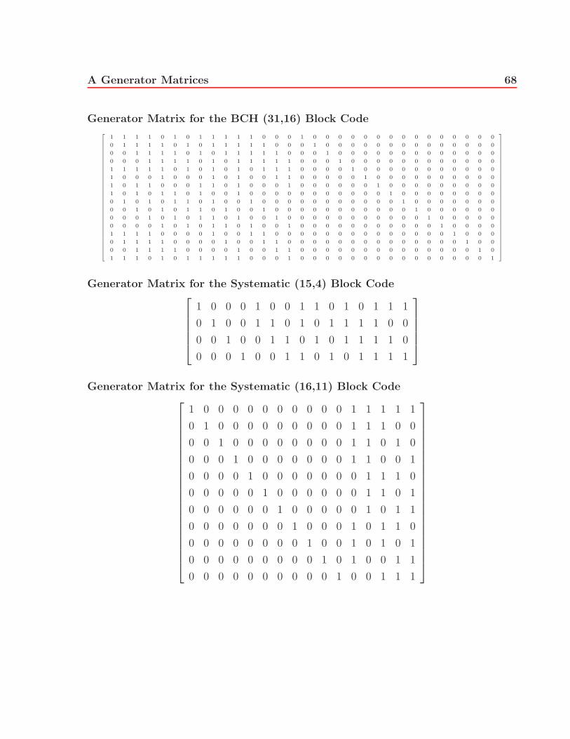
now consider two slightly more complex codes. Namely the Reed-Muller (16,11) and the
BCH (31,16) codes whose generator matrices can be found in appendix A. The first of
these two codes requires 252 edges and 149 states. This is still acceptable. However the
second code requires 196,604 edges and 131,069 states. In practical terms this means that
196,604 multiplications and 65,536 additions need to be performed to decode each block of
only 31 bits [5]. These numbers clearly show the impracticality of decoding certain block
codes using a minimal trellis. To solve this problem we propose the algorithm presented in
Page 22
2 Background 14
chapter 3 which reduces the number of states even further by selectively removing certain
codewords from the trellis.
2.3 Viterbi Decoding
Viterbi decoding is one of the most widespread decoding algorithm in use today. This
algorithm, proposed by Andrew J. Viterbi [6], a founder of the Qualcomm Corporation,
has since been studied at length and now has many variants. This section presents the
general idea behind the algorithm as well as some of the variants that have been developed.
The Viterbi algorithm is a computationally efficient way to find the maximum likelihood
sequence in a trellis given a received signal r = (r1, r2, ..., rn). The brute force approach to
finding this most likely codeword is to simply calculate a path metric for every path. A path
metric is a measurement of the reliability of a path and can be calculated in many different
ways. The Viterbi algorithm, as opposed to the brute force method, takes advantage of
the fact that paths sometimes merge. At the state where a merger occurs the algorithm
selects the path with the best metric as the survivor path. It is clear that all other paths
to the state in question are not optimal and thus continuing to calculate their metric only
wastes resources. These paths are therefore excluded from the list of possible most likely
codewords. Hence, only one survivor path and its associated metric need be saved at each
state. This procedure starts at σi and works its way to σf . Finally, the output of the
decoder is the path form σi to σf with the best path metric. If at a point of merger two
paths have equal metrics then one is chosen arbitrarily.
Different metrics can be chosen to determine the “best path” in the trellis, two of which
will be discussed shortly. It is important to note that the computation of the metric is the
operation in the Viterbi algorithm which is performed most often. For this reason the com-
plexity of the metric greatly affects the computational complexity of the overall algorithm.
Before going into more detailed explanations on metrics, we present the pseudo-code for
the Viterbi algorithm in figure 2.4.
In figure 2.4 we see that the metric operator can be used on either a state or and edge.
When it is used on a state it returns the value stored at that state; the Viterbi algorithm is
responsible for setting this value equal to the best metric from σi to the state in question.
When it is used on an edge, it simply returns the metric calculated for that edge.
Page 23
2 Background 15
Set initial state path metric = 0;
For( x = 1 ; x ≤ n, x ++){For(v ∈ Vx){
Select emin = argmine∈Ex,x+1 : end(e)=v
(metric(start(e)) + metric(e))
Set metric(v) = (metric(start(e)) + metric(e))Set path(v) = P(σi, end(emin))
}}
Fig. 2.4 Pseudo Code for the Viterbi Algorithm.
As we see from this pseudo-code the number of operations required in order to decode
the trellis is proportional to the number of edges in the trellis. It is for this reason that it is
important to select the simplest trellis representation possible for our trellis when wanting
to minimize decoding complexity. This also means that by removing states and edges from
this trellis it is possible to simplify decoding further but no guarantee can be made on
performance. There are many variations on the Viterbi algorithm depending on the type
of input and type of output that are available or are needed. A list of several of them as
well as some of their respective advantages is detailed below.
2.3.1 Hard Input, Hard Output
This is one of the simplest forms of the Viterbi algorithm, the output of which is a sequence
of ones and zeros with no reliability measurement. For this reason we say that the decoder
makes hard decisions. The input in this case is also a series of hard decisions (ones and
zeros) made by the detector based on the received signal before the Viterbi algorithm is
performed. This sequence does not take into account the trellis structure of the code and
thus the input need not be a valid codeword.
The metric used in this case is the Hamming distance and the codeword with the
smallest Hamming distance from the received signal is declared to be the most likely. This
implementation is computationally efficient due to the fact that the Hamming distance can
be calculated using a simple exclusive or operation. However in most real communication
systems soft information, i.e. information about the reliability of each input bit, is also
available to the decoder. This is not the case for this implementation because of the hard
Page 24
2 Background 16
decisions made on the input signal before decoding.
2.3.2 Soft Input, Hard Output
In this variation, the output of the Viterbi algorithm is still a sequence of ones and zeros
with no reliability measurements. However the reliability of the input signal is taken into
account when computing this output. For this reason we say that we have a soft input.
For example, if an antipodal ±1 BPSK signal is being sent over and AWGN channel, a
received value of +1.01 instills more certainty than a value of 0.17. Thus if ever it came
time to choose which of two values was in error, we would obviously choose the latter.
The metric used must be able to accommodate this new information. Since the square
of the Euclidian distance is the ML metric under AWGN conditions it is chosen instead of
the Hamming distance when soft information is available. It is calculated as follows:
dEuclidian = (r − x)2 (2.8)
Where r is the received value and x is the candidate. Once again the codeword with
the smallest distance from the received signal is declared most likely. By using this soft
information a gain of roughly 2 dB is achieved over hard input. This gain comes at the
price of a more complicated path metric. Again since the output is hard, no reliability
measurements of the output bits are available. This information would be useful when
further processing of the data is required.
2.3.3 SOVA or Soft Input, Soft Output
The SOVA or Soft Output Viterbi Algorithm is used when a reliability measurement of the
output bits is required. It was first proposed in [7]. This soft information can be used for
further processing such as in Turbo decoding applications. The log likelihood ratio is used
to measure this reliability at each depth of the trellis. For BPSK the ratio is given by [2]:
Lx = log
[( ∑c:cx=1
P (c|r))
/
( ∑c:cx=−1
P (c|r))]
(2.9)
In equation 2.9, P (c|r) is the probability that codeword c was sent given that vector r
was received. The MAP algorithm can calculate the exact values of Lx given the underlying
Page 25
2 Background 17
coding mechanism. However the computational complexity of this algorithm is extremely
high. The optimality of the MAP algorithm is foregone in SOVA in order to reduce the
complexity of the decoder. SOVA requires far fewer operations than MAP because it makes
uses of the following approximation [2]:
log
(N∑
j=1
δj
)≈ log
(max
j∈{1,2,...,N}{δj}
)(2.10)
Substituting Eq. 2.10 into Eq. 2.9 we obtain:
Lx ≈ log
(maxc:cx=1
P (c|r))− log
(max
c:cx=−1P (c|r)
)(2.11)
Eq. 2.11 has two terms. One corresponds to the maximum likelihood codeword. This is
the codeword that can be found using the conventional Viterbi algorithm. The other is the
most likely codeword which differs from this ML codeword at position x. The hard output of
the decoder is based on the sign of this difference. If the term on the left corresponds to the
maximum likelihood codeword then the sign of Lx will be positive and hard output of the
decoder will be 1. Otherwise the sign will be negative and the output will be a 0. In other
words the maximum likelihood codeword is also equal to (sign(L1), sign(L2), ..., sign(LN )).
As we can see the soft information is proportional to the reliability difference between
different paths in the trellis. In AWGN the reliability difference is defined as the difference
in the squared Euclidian distance separating the respective codewords (c1 & c2) from the
received signal.
reliability difference = ‖r − c1‖2 − ‖r − c2‖2 (2.12)
It is also possible to define the reliability difference between two paths merging at an
arbitrary state v ∈ Vx, denoted ∆v, as the difference between the cumulative correlation
metric of the most likely path from σi to v and that of the second most likely path with
the same start and end points. This difference is used to update the reliability, or soft
information, of each bit by the SOVA algorithm. Here the cumulative correlation metric
M(σi, vx) is defined as follows:
M(σi, vx) =
x∑i=1
ri · (2ci − 1) (2.13)
Page 26
2 Background 18
It is important to note that this metric is equivalent to the Euclidian distance men-
tioned in equation 2.8. By expanding the square we notice that maximizing the cumulative
correlation matrix is equivalent to minimizing the Euclidian distance. The SOVA algo-
rithm is very similar to the traditional Viterbi algorithm. Decoding is done is the same
order and the survivor paths are chosen in the same way. However, the SOVA algorithm
needs to keep track not only of the survivor paths but also of a list of their associated soft
information. This is where SOVA differs from conventional Viterbi. An additional step
needs to be performed each time two paths merge in order to update the soft information
of the surviving path. In other words the soft information for every bit in the merged path
needs to be updated taking into account the soft information found in both merging paths.
In order to explain the update procedure we rely on the following example. Suppose
that two paths p1 and p2 merge at state v where v ∈ Vx. We will denote the soft information
vector associated to p1 and p2 as Ll(v) = {Ll1, L
l1, ..., L
lx−1} where l ∈ {1, 2} corresponds to
the path number. For ease of discussion we will assume, without loss of generality, that p1 is
selected as the survivor path. The first thing to do in order to update the soft information
is to set Lmergedx = ∆v since this latest bit is the deciding factor between p1 and p2 and the
difference between them is ∆v. Then we need to update the rest of Lmerged(v). Suppose
that the first i − 1 values have already been updated. We would like to update the ith
value, namely Lmergedi . This value is linked to the bit at position i where i < x.
There are two possible scenarios for this update and each requires a different update
function. In the first scenario the bit at position i in p1 is different than the one in p2. In
other words the paths do not agree on the bit at this position. It follows that Lmergedi cannot
be greater than the reliability difference between the two paths, since this would imply that
we are more sure about the bit at position i than we are about the choice between p1 and
p2, which is a contradiction. Also, if this bit is less likely than the reliability difference,
i.e. L1i < ∆v, then Lmerged
i cannot be larger then L1i since this value was determined by a
previous merger between p1 and a path for which the reliability difference was even smaller
than the one in progress. In other words if an error occurs at this position it is more likely
that the error will be due to the previous merger than the one in progress. Thus Lmergedi (v)
is updated as follows when p1(i) �= p2(i) [2]:
Lmergedi (v) = min{∆v, L1
i } (2.14)
Page 27
2 Background 19
In the second situation, the two paths do agree on the bit at position i. The update
function must therefore be different. For the same reasons as previously stated, Lmergedi
cannot be greater than the current L1i . However it could be smaller due to p2’s uncertainty
about bit i, denoted L2i , . We must therefore also take this uncertainty into account,
with an additional penalty of ∆v due to the reliability difference between the two paths,
when updating the soft information of the survivor path. Thus the update function when
p1(i) = p2(i) is [2]:
Lmergedi = min{∆v + L2
i , L1i } (2.15)
This procedure is repeated for each bit in the surviving path when a merger occurs
in the decoding process. The final output of the algorithm is the sole surviving path and
Lmerged(σf ). This vector contains the approximations of the log likelihood ratios we were
trying to obtain. A sliding window version of the SOVA algorithm can be found in [8]. We
conclude this section with the presentation of the pseudo-code for the SOVA algorithm.
This algorithm is very similar to the Viterbi algorithm but includes an additional loop
which updates all the soft values for the new merged path based on the previous values and
the reliability difference between the two merging paths. This loop considerably increases
the overall decoding complexity.
Set initial state path metric = 0;
For( x = 1 ; x ≤ n, x ++){For(v ∈ Vx){
Select the surviving path and calculate ∆v
Update the path and set Lmergedx = ∆v
For( a = 0 ; a < x ; a++){If(p1(a) �= p2(a))
Set Lmergeda (v) = min{∆v, L1
a}Else If(p1(a) = p2(a))
Set Lmergeda = min{∆v + L2
a, L1a}
}}
}Fig. 2.5 Pseudo Code for the SOVA Algorithm.
Page 28
2 Background 20
2.4 Trellis Reduction
Reducing the size of the trellis to a usable size is one of the main focuses of this thesis.
The innovative and efficient way that we developed to simplify trellises based on the re-
ceived signal is presented in chapter 3 and in our paper [9]. Before presenting it however
we will first examine methods that have already been developed by other authors. These
simplification methods can be found in [10], [11], [12] and [13]; two of which are presented
in greater detail in this chapter. In particular we explore the main idea behind the simpli-
fication process. All methods achieve a reduction in complexity, but each does so by very
different means.
In general, algorithms which attempt to perform maximum likelihood decoding on the
full trellis representation of block codes spend most of their time calculating path metrics
for paths that are very unlikely. However by foregoing optimality it is possible to develop
many efficient schemes that can produce near-optimum performance. Presented here are
two such sub-optimal methods. Both perform decoding on a reduced, or pruned, trellis.
However their reduced trellises are not constructed in the same way. It is interesting to
examine these schemes in order to understand the ways in which these methods differ from
the one proposed in this work.
2.4.1 Low Weight Sub-Trellises
The first method, proposed in [10], is based on the construction of low weight sub-trellises.
Before presenting this method we must first define the weight profile of a binary code C.
The weight profile w = {0, w1, w2, ...} of C is defined as the set of all distinct weights
of the codewords in the code book. Here, wa < wa+1 and w1, which can also be written
wmin, is known as the minimal (non-zero) weight of C.
The weight(wa) sub-trellis is defined as a trellis which is composed of all codewords of
weight wa in the code book. The sub-trellis associated with wmin is known as the minimal
weight trellis. It is also possible to define the weight(w1 : wa)-subtrellis, this sub-trellis
contains all codewords whose weights are between w1 and wa and also includes the all-zero
vector.
Decoding using the low weight sub-trellis method starts by generating the weight(w1 :
wa)-subtrellis. The choice of a will be explained shortly. This sub-trellis is said to be
centered around the all-zero codeword since the weights also correspond to the Hamming
Page 29
2 Background 21
distances between the other codewords and this vector. Next, hard decision decoding is
performed on the received signal in order to obtain a first hard-decision ML estimate z.
Then, the search for the most likely codeword is performed using the weight(w1 : wa)-
subtrellis centered around z instead of using the full trellis. Centering the weight(w1 :
wa)-subtrellis around z is accomplished by simply adding this vector to the paths in the
weight(w1 : wa)-subtrellis centered around the all-zero codeword. Reducing the size of the
trellis in this way results in considerable computational savings. However if the most likely
codeword in the full trellis is not in the pruned trellis a loss in optimality occurs. For this
reason we say that this method is sub-optimal.
Determining an appropriate value for a is an important part of this method since this
parameter determines the size of the pruned trellis and thus the computational complexity
of the decoding process. In general a is chosen to be small, hence the name “low weight
sub-trellis”. The smaller the value of a, the fewer codewords are present in the trellis since
all codewords that differ from the received codeword in more then wa positions are pruned
from the trellis. When a = 1 the search is performed on the minimal weight trellis.
However a value of a which is too low can lead to poor performance.
2.4.2 Chase Decoding
Another method of reducing the size of a block code’s trellis to a usable size was proposed
by Chase in [11]. His method is based on the idea that if errors in transmission have
occurred they most likely have occurred in the least reliable bits of the received sequence.
By selecting the a least reliable bits from the received sequence it is possible to create
2a error test patterns. These patterns are more likely to occur than others due to the low
reliability of the received signal at these positions. Once again the choice of a determines
the complexity of decoding. These test patterns are then used in order to decode the re-
ceived sequence. In this way the computational complexity of decoding can be dramatically
reduced. Chase demonstrated that his algorithm achieves good performance by using these
error patterns and by selecting a = dmin
2.
2.5 Turbo Codes
Turbo codes are a type of FEC that have very strong error correcting capabilities. Many
other codes have this characteristic yet most result in decoder solutions which are far too
Page 30
2 Background 22
complex to implement. Turbo codes avoid this problem by combining two relatively simple
codes rather than using one very complex code. This combination results in long powerful
codes which can be decoded using a relatively simple decoder.
Although there exists many different ways to select and combine the constituent codes,
this work will focus primarily on concatenated block codes. This section is based on the in
depth presentation of the turbo codes presented in [8] and [14] .
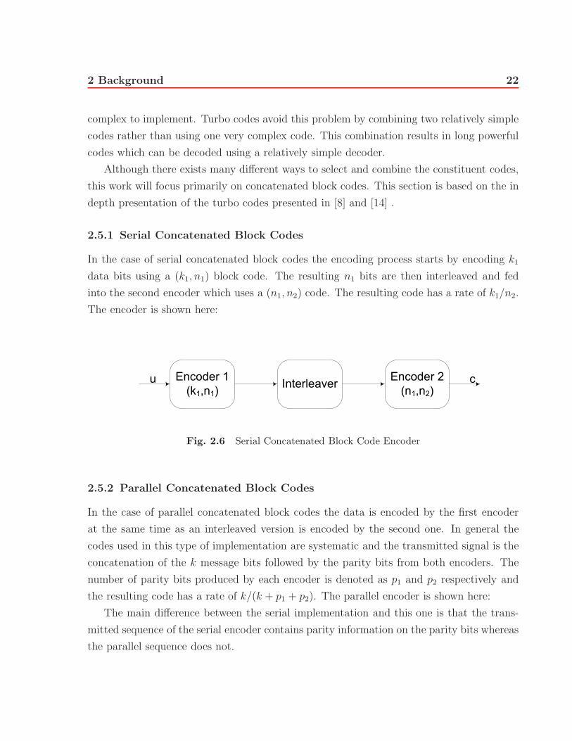
2.5.1 Serial Concatenated Block Codes
In the case of serial concatenated block codes the encoding process starts by encoding k1
data bits using a (k1, n1) block code. The resulting n1 bits are then interleaved and fed
into the second encoder which uses a (n1, n2) code. The resulting code has a rate of k1/n2.
The encoder is shown here:
Encoder 1
(k1,n1)Interleaver
Encoder 2
(n1,n2)u c
Fig. 2.6 Serial Concatenated Block Code Encoder
2.5.2 Parallel Concatenated Block Codes
In the case of parallel concatenated block codes the data is encoded by the first encoder
at the same time as an interleaved version is encoded by the second one. In general the
codes used in this type of implementation are systematic and the transmitted signal is the
concatenation of the k message bits followed by the parity bits from both encoders. The
number of parity bits produced by each encoder is denoted as p1 and p2 respectively and
the resulting code has a rate of k/(k + p1 + p2). The parallel encoder is shown here:
The main difference between the serial implementation and this one is that the trans-
mitted sequence of the serial encoder contains parity information on the parity bits whereas
the parallel sequence does not.
Page 31
2 Background 23
Encoder 1
(k1,n1)
Encoder 2
(k2,n2)
Interleaver
u u
P1
P2
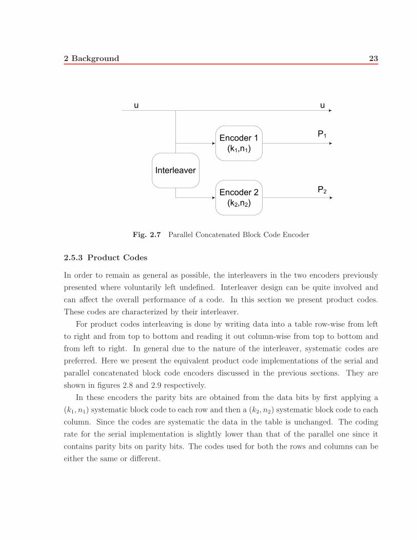
Fig. 2.7 Parallel Concatenated Block Code Encoder
2.5.3 Product Codes
In order to remain as general as possible, the interleavers in the two encoders previously
presented where voluntarily left undefined. Interleaver design can be quite involved and
can affect the overall performance of a code. In this section we present product codes.
These codes are characterized by their interleaver.
For product codes interleaving is done by writing data into a table row-wise from left
to right and from top to bottom and reading it out column-wise from top to bottom and
from left to right. In general due to the nature of the interleaver, systematic codes are
preferred. Here we present the equivalent product code implementations of the serial and
parallel concatenated block code encoders discussed in the previous sections. They are
shown in figures 2.8 and 2.9 respectively.
In these encoders the parity bits are obtained from the data bits by first applying a
(k1, n1) systematic block code to each row and then a (k2, n2) systematic block code to each
column. Since the codes are systematic the data in the table is unchanged. The coding
rate for the serial implementation is slightly lower than that of the parallel one since it
contains parity bits on parity bits. The codes used for both the rows and columns can be
either the same or different.
Page 32
2 Background 24
Data Bits
Parity Bits
Parity
Bits
k1 n1-k1
k2
n2-k2
Parity
On
Parity
Fig. 2.8 Serial Concatenated Product Code Encoder.
Data Bits
Parity Bits
Parity
Bits
k1 n1-k1
k2
n2-k2
Fig. 2.9 Parallel Concatenated Product Block Code Encoder.
Page 33
2 Background 25
2.5.4 Turbo Decoding
Before going into the specific implementations of turbo decoders we will first explain the
underlying idea. Turbo decoding is accomplished by iteratively using information gained
during the decoding of one code to help in the decoding of the next. In other words
information is fed back into the decoder in much the same way as a turbo compressor
sends air back into the motor of an automobile, hence the name turbo codes.
Consider the case of a product code in which the rows of the table are decoded first.
This decoding results in new information being available to the decoder. This information
can then be used in combination with the channel information to decode the columns. This
in turn results in new information which can be used to re-decode the rows, and so on and
so forth. This is much like solving a crossword puzzle. Each new word found in the rows
allows you to solve words in the columns and vice versa. Finally after a set number of
iterations or another stopping criterion is met the final version of the data is output.
This procedure is illustrated in the next figure. It should be noted that this iterative
decoding process performs significantly better when the decoders output soft values instead
of hard decisions. It is for this reason that outputs of the decoders in the diagram presented
below are log likelihood ratios. Specifically figure 2.10 represents the turbo decoder for the
parallel encoder presented in figure 2.7.
SISO
Decoder 1SISO
Decoder 2
Deinterleaver Interleaver
Interleaver
& Hard
DecisionsDeinterleaver
)ˆ(1 uLe
)ˆ(2 uLe
0)(uL
rLc
)ˆ(2 uL u
)ˆ(1 uL
Fig. 2.10 Parallel Iterative Turbo Decoder
Here U and U are the k × k matrices containing the transmitted data and the esti-
mates of the transmitted data respectively in matrix form. They correspond to the k × k
information bits in figure 2.9. L(U) is the a priori log likelihood ratio of the data, L1e(U)
Page 34
2 Background 26
and L2e(U) are the extrinsic information from decoder 1 and decoder 2 respectively, R is
the k × k matrix containing the received signal and Lc is called the reliability value of
the channel. This reliability factor is linked to the signal to noise ratio and the fading
attenuation. It is equal to 4aEs
N0, where a is the fading. For AWGN channels a = 1 and Es
N0
is the SNR estimate at the receiver.
In order to estimate the transmitted data U the decoder uses all three sources of infor-
mation at its disposal. They are: the information from the channel, the a priori knowledge
about the bits and the extrinsic information obtained during decoding. SISO Decoder 1 in
figure 2.10 has two different outputs. The first L1(U) is the estimate based on the three
sources of information just mentioned. It is the main output from the decoder. This output
can be broken down as follows [14]:
L(U) = LcR + L(U) + Le(U) (2.16)
During the first iteration we set L(U) = 0 if no a priori information is available. The
second output of the decoder is L1e(U), this output is the information that was gained during
decoding and is known as extrinsic information, it is found by subtracting the information
gained via the channel and that known a priori from the estimate L(U) output by the soft-
output decoders. It is important that extrinsic information not be used more than once
due to the danger of positive feed back. For the same reason we do not use the a priori
information more than once either. Instead the extrinsic information from the previous
decoder is used as the a priori information for the current decoder. The only exception
of course is the very first iteration. Thus, after the first iteration, when the switch in
figure 2.10 is set to the output of the interleaver rather then L(U), we see that extrinsic
information from the most recent iteration can be written as [14]:
L1e(U) = L1(U) − LcR − L2
e(U) (2.17)
L2e(U) = L2(U) − LcR − L2
e(U) (2.18)
At each iteration this update is performed and the process is terminated once a set
number of iterations have been completed or another stopping criterion has been met. The
final output is obtained by making hard decisions on the sign of L2(U), which combines
channel information as well as the extrinsic information from both decoders.
Page 35
2 Background 27
This information on turbo decoders as well as the information contained in the other
sections of this chapter is the foundation upon which we have developed our innovative
algorithms. The topics covered in this chapter are used extensively throughout this entire
thesis. Now that the foundations have been laid the next chapiter presents the work that
we have done which brings together these various subjects.
Page 36
28
Chapter 3
Selective Trellis Pruning
When channel conditions are favorable, higher coding rates are desired in order to increase
channel throughput. Recall that at these rates the performance of convolutional codes
suffers due to the use of puncturing. For this reason designers look to block codes for a better
solution. However, their extremely large trellis representations makes them impractical to
decode.
In this chapter we examine a way to reduce the size of the trellis representation to
usable sizes while still maintaining near-optimal performance. This is done by way of trel-
lis pruning. Pruning a trellis consists of removing various edges and states from it thus
reducing the corresponding decoding complexity. However this procedure also results in
the fact that trellis no longer represents all codewords in the code book. The decoder can
therefore no longer guarantee that the maximum a posteriori probability (MAP) codeword
will be found since it may have been removed from the trellis. For this reason we see that
removing edges and states at random can be disastrous with respect to performance. In
order to reduce the risk that the MAP codeword be pruned from the trellis we perform
selective trellis pruning. Selective pruning consists in intelligently choosing which code-
words to remove based on the information available to the decoder. In this way we hope to
remove many states and edges from the trellis without removing the MAP codeword. In
the case of our algorithm, pruning in our trellis is based on the soft information contained
in the received signal. The price to pay for this reduction in complexity is obviously a loss
in performance. However when the pruning is done correctly, the MAP codeword is rarely
pruned, and this loss can be quite small.
Page 37
3 Selective Trellis Pruning 29
This chapter focuses on our selective trellis pruning algorithm. It will be presented in
two parts. The part first focuses on how to choose the codewords that can be pruned. The
second details the innovative way in which these codewords are removed from the trellis.
This last part is of the utmost importance since the overall computational complexity of
the algorithm depends greatly on the efficiency of this removal. Finally we explain how
this algorithm can be used in the context of a turbo decoder.
3.1 Selective Trellis Pruning
The presentation of the algorithm, although having two main parts (namely: codeword
selection and codeword removal), will be subdivided into five subsections. The first three
are related to codeword selection. They will respectively focus on the selection of the bits
to be simplified, the order in which to simplify them and how many should be simplified.
Codeword removal will be divided in two subsections, each explaining a different way to
prune the selected codewords from the trellis.
3.1.1 Bit Selection
In order to reduce the size of the trellis certain codewords must be removed from the trellis.
The selection of these codewords is key to the performance of the decoding algorithm. For
this reason codewords cannot be eliminated at random but must be carefully selected
based on information available to the decoder. There are two sources of information that
the decoder can take advantage of. They are the a priori probabilities of the transmitted
bits and received signal itself. Based on this information it is possible to make certain
assumptions and thus eliminate certain codewords.
It is possible to simplify the trellis of a code by not including codewords which, based on
the a priori information, are very unlikely. However due to the equiprobable nature of the
codewords in most real systems, using this information yields few simplifications. This is
because few codewords are very unlikely a priori. For this reason most methods developed
rely on the received signal in order to prune the trellis.
The two methods presented in the previous chapter are perfect examples. The low
weight sub-trellis method, seen in section 2.4.1, bases its simplification on the hard decision
sequence of the received signal which it uses to construct the weight(w1 : wa)-subtrellis.
Thus all codewords not belonging to this sub-trellis are removed as possible candidates.
Page 38
3 Selective Trellis Pruning 30
The method does not however take into account the reliability of each individual bit. The
Chase algorithm, presented in section 2.4.2, on the other hand does consider these individual
reliabilities. Based on the x least likely bits of the received signal it selects its candidates.
The method we propose is similar to the Chase algorithm in the sense that it considers
the likelihood of bits individually. It is based on the simple idea that most likely bits in the
received signal are least likely to be in error. Thus by assuming them to be known one can
simplify decoding without affecting performance significantly. This is similar to the Chase
algorithm. The difference between the two being that Chase varies the x least likely bits
to generate test patterns while ours makes hard decisions on the x most likely ones. By
fully determining these bits, codewords which do not respect these determinations are no
longer needed and can be pruned from the trellis.
The terms likelihood and likely have been used frequently in this chapter when refer-
ring to bits in the received sequence. These terms refer to the likelihood ratio for each
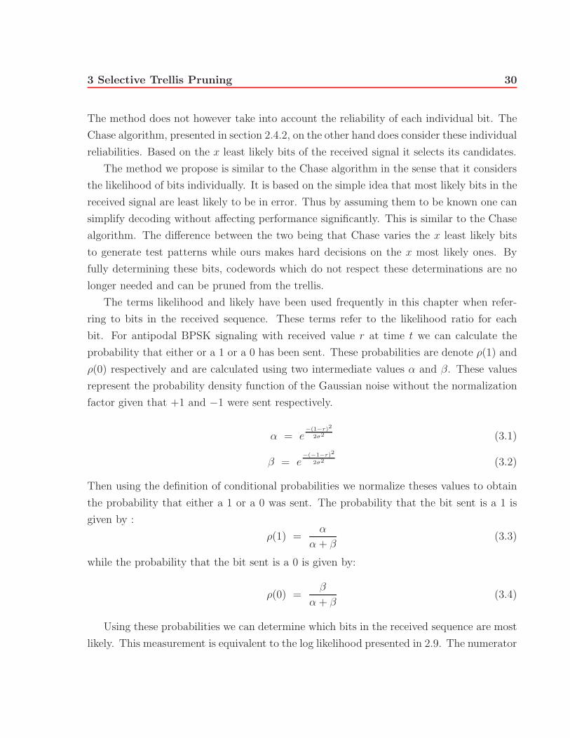
bit. For antipodal BPSK signaling with received value r at time t we can calculate the
probability that either or a 1 or a 0 has been sent. These probabilities are denote ρ(1) and
ρ(0) respectively and are calculated using two intermediate values α and β. These values
represent the probability density function of the Gaussian noise without the normalization
factor given that +1 and −1 were sent respectively.
α = e−(1−r)2
2σ2 (3.1)
β = e−(−1−r)2
2σ2 (3.2)
Then using the definition of conditional probabilities we normalize theses values to obtain
the probability that either a 1 or a 0 was sent. The probability that the bit sent is a 1 is
given by :
ρ(1) =α
α + β(3.3)
while the probability that the bit sent is a 0 is given by:
ρ(0) =β
α + β(3.4)
Using these probabilities we can determine which bits in the received sequence are most
likely. This measurement is equivalent to the log likelihood presented in 2.9. The numerator
Page 39
3 Selective Trellis Pruning 31
in 2.9 simply corresponds to ρ(1) while the denominator corresponds to ρ(0) which is also
equal to 1 − ρ(1). For example if ρ(1) = 0.999 then the equivalent log likelihood ratio is
given by:
Lx = log [(0.999) / (1 − 0.999)] = 2.999 (3.5)
We therefore conclude that theses measurements are interchangeable. These equations
do not include the terms that would factor in the a priori knowledge [15], therefore they
assume that the symbols are equiprobable. This same assumption is made when the a
priori knowledge is unknown, which is the case in most real systems.
The likelihood of each bits was chosen in order to determine which bits could be declared
known in our algorithm. Before selecting this characteristic however, we also examined
other possibilities. Amongst other things, we examined if simplifying two bit near each other
was better than simplifying two bits further apart. This turned out to be very dependent on
the generator matrix and was not useful when trying to implement a general algorithm. We
also explored the possibility that certain types of bits might yield greater performance gains
than others. In other words, was there more to gain from the simplification of a systematic
than a redundant bit or vice versa. Several tests were run in order to determine if this could
be taken advantage of. It was found that when a systematic bit was simplified performance
suffered marginally less then when a redundant bit was chosen. However we determined
that the increase in complexity required at the decoder was not worth the limited gain in
performance. For this reason no further effort was made to push this concept further. The
tests as well as the results that were used to make this determination are presented in the
chapter 4.
3.1.2 Simplification Order
When more than one bit can be simplified, and only a given number of simplifications
may be performed, it is important to determine wether or not the order of simplification is
important and if so which order should be chosen. We based our order on two criteria. The
first is the complexity of the pruned trellis. We chose this criterion because it determines the
overall computational complexity of the decoding algorithm. Based on this criterion, bits
that reduce the size of the trellis the most should be selected before bits that simplify the
trellis less. The second criterion is performance. By this we mean selecting a simplification
Page 40
3 Selective Trellis Pruning 32
order that will affect performance as little as possible. Presented now are the reasons,
based on these two criteria, which motivated the choice of our simplification order.
Recall that the goal of our algorithm is to minimize complexity by reducing the size of
the trellis. Given equiprobable symbols in the codewords, trellis size is reduced by a given
amount independently of which simplification order is chosen. Therefore, with respect to
our complexity minimization criterion, the order of simplification is irrelevant. This means
that we can choose the order of simplification based solely on the criterion of performance.
The performance of a decoding algorithm is based on the amount of information avail-
able to the decoder and how it is used. When decoding is performed on the full trellis we
say that it is optimal because it makes use of all the information at its disposal. However,
making simplifications implies a certain loss of information. In other words, each time
we remove a codeword from the trellis we remove information from the system. There-
fore the goal when performing pruning is to remove as little information as possible. This
also implies that some codewords contain more information than others. These codewords
were determined to be the ones nearest the received signal. This can be understood by
considering the fact that the act of simplifying bits is equivalent to making hard decisions
on their values. It is obvious that less information is lost when quantizing 0.99 = 1 then
when quantizing 0.55 = 1. For this same reason simplifications should not be made which
contradict the received signal, i.e. setting a received value of −0.1 = +1 should not be
selected over setting it to −1.
Based on the criteria set forth, we determined that the optimal simplification order is
based on the likelihood of the received bits. Thus simplification should be made in direction
of the received signal in decreasing order of likelihood, from most likely to least likely. This
order ensures that trellis size is reduced as much as possible while not removing information
unnecessarily.
This order has other advantages as well. Suppose that some bits in the received se-
quence are in error. Knowing that simplifications are always made in the same direction as
the received bit, they inevitably lead to errors in the decoded sequence since these simpli-
fications permanently flip received bits. In other words, the transmitted codeword in these
cases is pruned from the trellis. It is also possible that the simplification of two different
bits lead to conflicting simplifications in the trellis. For example, suppose we make two
simplifications. First we simplify the a bit at position x1. After pruning the trellis we note
that all remaining codewords have a value of 0 at position x2. Now suppose that the next
Page 41
3 Selective Trellis Pruning 33
simplification that is to be made is to set the bit at position x2 = 1. This is obviously a
conflicting simplification. If carried out, all codewords would be pruned from the trellis and
the trellis would be empty. This is impossible since a codeword was obviously transmitted
and we must therefore conclude that one of our simplifications is in error. Simplifying bits
in order of likelihood ensures that in the case of conflicting simplifications the most likely
simplification is always performed first. Furthermore, if ever a conflicting simplification
were to occur, it would simply be ignored. This is because any such simplification would
conflict with a previous simplification which was based on a more likely bit. The second
simplification is therefore considered to be erroneous.
3.1.3 Amount of simplification
Once the order of simplification has been determined, it is important to determine the
amount of simplifications that should be made. The low-weight sub-trellis algorithm deter-
mines the amount of simplifications to be made via the selection of simplification weight wa
and the Chase algorithm determines the number of least significant bits that will be used
to create its test patterns. The algorithm we propose must select how many bits can be
declared known in the received sequence. The more bits that are chosen the more simpli-
fications will be performed. However as simplifications are made, performance inevitably
suffers. For this reason the choice of how many simplifications are made represents a
trade-off between complexity and performance.
It is possible with our algorithm to trade as much or as little complexity as one desires.
Specifically, by making no simplifications the algorithm is equivalent to the regular Viterbi
algorithm and thus achieves ML optimal performance with regards to the code in use. On
the other hand if all bits are declared known without regard for the trellis structure and
hard decisions are made on every bit, the algorithm behaves in same way as un-coded
BPSK. It is thus possible to operate anywhere between optimal performance and that of
un-coded BPSK. For this reason there is no set answer to how much complexity can be
saved. The answer depends only on the performance the user would like to achieve and
what he is willing to sacrifice. However it is possible for two simplification thresholds to
yield very similar performance for a given point of operation while using a very different
number of operations. We will now discuss how we chose what we feel is the best trade-off
between performance and computational complexity.
Page 42
3 Selective Trellis Pruning 34
One possible choice we explores was to select a set number of bits to be simplified in
each block. This is similar to what the Chase and the low-weight sub-trellis methods do.
They select the optimal value of wa or the optimum number or the least likely bits to
be used for a given operating point. This could be implemented with our simplification
scheme by simplifying a set number of the most likelihood bits. For example we can choose
to only simplify the most certain bit in each received block. This roughly results, when
bits are equiprobable, in half the codewords being removed from the trellis, a significant
saving. The question that then needed to be asked wa whether or not more bits could
be simplified. Ideally we wanted to simplify as many bits as possible while not affecting
performance significantly.
This idea leads to the possibility of selecting a different number of bits to be simplified
in each block. This solution is more dynamic. Using this scheme it is possible to tailor the
simplifications to each received block. In other words we take advantage of the soft infor-
mation in the received signal not only in the decoding process but also in the simplification
process. Previous works in this area do not make use of this information.
In order to take advantage of the soft information in the simplification process in an
efficient way we introduced a simplification threshold, denoted θ. θ represents the minimum
probability which a bit can have and still be simplified. In other words if either ρ(1) or ρ(0)
is above the simplification threshold θ then the bit at time t can be assumed known as either
a 1 or a 0 respectively. It is logical that the choice of the number of bits to be simplified is
based on the same criterion that was used to determine the order of simplification.
It is clear that by using this type of threshold the amount of simplifications that occur
in each block depends on the received signal. The more bits above the threshold, the more
simplifications can be made. The threshold also adds the assurance that although many
simplifications may be made the decoder has a certain degree of confidence in each one.
Alternatively if the received signal is particulary poor, it is possible that no simplifications
be made. When this is the case however, full trellis decoding is performed, which, from
a performance point of view, is a good idea when the received values are unclear. It
is important to note that when only one codeword remains in the trellis this codeword is
output and the simplification process stops. This is not equivalent to making hard decisions
on the received signal since the trellis structure is taken into account. This guaranties that
the output of the decoder will be a valid codeword. This is not the case with un-coded
BPSK.
Page 43
3 Selective Trellis Pruning 35
The choice of the simplification threshold is an important part of the algorithm. Se-
lecting a threshold which is too low will lead to unwanted performance degradation while
selecting one that is too high diminished the computational savings. The next question is
whether how to find an appropriate threshold exists. It was determined by simulation that
some thresholds outperform others, these threshold values depend on many factors such as
the code in use, the signal to noise level of the operating point as well as the desired bit
error rate. This will be discussed in much greater detail in the section 4.2.4.
We also studied the behavior of our algorithm under different operating conditions. We
studied the effects of choosing a very low threshold as well as one that was very high.
In particular we examined the effects of the simplification threshold on the performance
of different codes establishing links between their performance and various block code
characteristics. A full list of the tests conducted and the corresponding results are presented
in chapter 4.
The next section focuses on the implementation issues related to our algorithm. However
before going into these details we first summarize the likelihood based selective trellis
pruning algorithm developed in figure 3.1.3.
Pseudo Code
1. Calculate ρ for all n bits
2. Select x as the unsimplified bit with the greatest ρ
3. While (ρx > θ and S �= {} ) repeat 4 & 5
4. Prune the trellis
5. Select x as the unsimplified bit with the next greatest ρ
6. Decode with Viterbi or SOVA using the pruned trellis
Fig. 3.1 Pseudo Code of the selective trellis pruning algorithm
Page 44
3 Selective Trellis Pruning 36
3.1.4 Implementation Issues
The algorithm proposed can efficiently select the codewords that need to be removed from
the trellis in order to reduce the computational complexity while affecting performance as
little as possible. However, several steps were added to the decoding process. They are: the
computation of the probabilities for each bit, the selection of the bits to be simplified and
the removal of codewords from the trellis. If these operations require as many operations
as they save in the decoding process, no overall savings are achieved. For this reason it is
important to consider the complexity of these extra steps.
The first two steps are quite straightforward. They do not increase complexity substan-
tially since they require only a few multiplications and comparisons. The total number of
operations is on the order of n since they are only performed once for each bit in the n bit
received signal. For this reason we conclude that these steps will not adversely affect the
overall complexity of our decoding algorithm.
On the other hand the fourth step in the pseudo code, the pruning of the trellis, might
require a very larger number of operations if implemented inefficiently. This is because the
number of codewords that need to be removed is on the order of 2k. This number grows
exponentially as the size of the code increases. For this reason it is very important to have
en efficient pruning algorithm. In the course of this work, two algorithms for obtaining the
pruned trellis were developed.
The first method is the most straightforward and intuitive. It begins by generating the
full minimal trellis representation of the code directly from its generator matrix using the
method proposed in [5]. Recall that this trellis contains all valid codewords and employs
the minimal number of edges and states. A recursive pruning function is then called with
the first bit in the simplification order as a parameter. This function removes all edges at
simplification depth that have labels opposite to the one of the bit being simplified. The
removal of these edges sometimes results in states becoming unneeded. Unneeded states
are states which no longer have at least one edge entering and leaving them, they are thus
not part of any codeword and can be pruned. All edges attached to an unneeded state can
also be removed. This can lead to removal of more states and so on and so forth. It is for
this reason that the pruning algorithm is implemented recursively. This function is called
in order to simplify all bits in the simplification order above the likelihood threshold. After
the last bit is simplified the trellis is in the desired pruned form. Decoding can then be
Page 45
3 Selective Trellis Pruning 37
performed on this trellis.
This method presents several drawbacks. The first is due to the complexity and the
sheer number of times that the recursive function must be called. This function can only
remove one edge or one state at a time and only after a series of tests have been performed.
These tests insure that the current element should in fact be removed and also identifies
other elements that might need to be pruned. The tests also verify that at least one valid
codeword is still present in the trellis after the removal of the selected elements is completed.
Another problem is that once a block is decoded the full trellis must be restored. Trellis
restoration is required since the simplifications performed on each block are not necessarily
the same. The problem is that this restoration can also requires a fair amount of operations
even when it is accomplished by using a copy of a previously stored version of the full trellis.
This is especially true when the size of the full trellis is large. Using this method of pruning,
observe that the trellis always starts and ends in its full version . A lot of unnecessary work
is thus put into reducing and then restoring the trellis.
Due to these problems it was determined that a more efficient way of pruning the trellis
should be found. The innovative method for pruning the trellis which we developed and
which avoids these problems is presented in the next section.
3.1.5 Trellis Pruning via Generator Matrix Simplification
Recall that the problem with the recursive pruning algorithm is the number of wasted
operations during the reduction and restoration of the full trellis. The solution we propose
avoids these problems by building a pruned trellis directly. In other words the full trellis
no longer has to be pruned and then restored each time a block is decoded. Instead only
a pruned version has to be constructed.
We found that it was possible to construct the pruned trellis directly from a modified
generator matrix using the same algorithm previously used to obtain the full minimal trellis.
The inspiration for our solution came from the fact that if the full trellis could be built
directly from a generator matrix, so too could the pruned trellis. The matrix used however
was not the generator matrix G but a modified version of this matrix. Our method also
requires a translation vector denoted e. This is due to the fact that matrices can only
represent linear codes, and, simplifications that set the value of a bit to 1 lead to non-linear
codes. We did however choose G as a starting point since a pruned trellis represents a coset
Page 46
3 Selective Trellis Pruning 38
of a sub-code of C. In other words this method does not simplify the trellis, it simplifies
the generator matrix. In this way, the problem of wasted operations during the pruning
and restoration of the trellis are solved.
This way of simplifying is clearly better than the previous method because of the fact
that simplifications take place at the generator matrix level. Therefore we only need to
generate a trellis which contains 2k−a codewords where a is the number of simplifications
made. This represents a significant reduction in complexity when the value of a is large.
Even when a = 1 savings are significant since the number of codewords is reduced by 50%.
However when no simplification are made our method must generate a full trellis. In this
worst case scenario the recursive algorithm is superior since its trellis is already in its final
form. On average however, when an appropriate simplification threshold is in use, the value
of a > 1.
The procedure used to modify the generator matrix of C and obtain the translation
vector will be explained in detail shortly. Before proceeding however we first expand the
idea behind our method in order to facilitate the understanding of the mathematics. We
first discuss the necessity of the the translation vector. To illustrate, suppose we would like
to find the matrix that can generate the pruned trellis in which we have declared the ith bit
to be equal to 1. Mathematically this simplification constrains all codewords to have a 1
at position i. This also means that the all-zero codeword will not be in the pruned trellis.
However any matrix multiplied by the all-zero input message equals the all-zero codeword.
For this reason we see that a generator matrix alone cannot represent the codewords in the
pruned trellis. It is for this reason that the translation vector is required.
The simplified generator matrix’s role in our algorithm is not to represent the coset of
the sub-code, but the sub-code. This is the version in which all of the simplified codewords
are present but have all been translated by the same vector e, the coset leader. In this way
the sub-code can be obtained by simply translating the sub-code by the translation vector.
The constrained codewords can then be constructed using the translation vector e and the
modified generator matrix.
Let G =(
gT1
gT2
... gTn
)be the generator matrix of a kxn code, where gT
iis kx1.
We are looking for a way to constrain a code bit.
Let i1, ..., iγ be the set of locations where we want to constrain the bits : {i1, ..., iγ} ⊆{1, ..., n}.
Page 47
3 Selective Trellis Pruning 39
Let α1, ..., αγ be the corresponding constrained values, i.e., we are looking for a parametriza-
tion of codewords :
S = {c ∈ {0, 1}n : ∃ u ∈ {0, 1}k : c = uG and cij = αj, j = 1, ..., γ} (3.6)
This is possible with a series of generator matrices G(j) and vectors e(j);
The procedure to determine G(j) and e(j) is the following:
1. Given G(j−1) with (G(0) .= G) compute a matrix P(j) such that
P(j)g(j−1)T
ij= 0 (3.7)
If g(j−1)Tij
= 0, then:
P(j) = Ikj−1 x kj−1(3.8)
otherwise: P(j) is (kj−1 x kj−1), where kj−1 is the number of rows of G(j−1).
2. It is then clear that :
∀ u(j) ∈ {0, 1}kj : u(j)P(j)G(j−1) = 0 (3.9)
So {(u(j)P(j)) : u(j) ∈ {0, 1}kj} generates all possible information words such that
they result in the ij-th bit of the codeword being 0.
3. Pick e(j) ∈ {0, 1}kj−1 such that
α(j) .=
e(j)G(j−1), if j = 1;
e(j)G(j−1) +j−1∑r=1
e(r)G(r−1), otherwise(3.10)
has its ij-th bit equal to (α(j))ij := αj .
This is easy to do :
Page 48
3 Selective Trellis Pruning 40
• if j = 1 or αj = (j−1∑r=1
e(r)G(r−1))ij : e(j) = 0 will do.
• if αj �= (j−1∑r=1
e(r)G(r−1))ij then choose e(j) = g(j−1)Ti
where (g(j−1)Ti
)ij = 1.
4. Then , all codewords of G with bits i1, ..., iγ equal to α1, ..., αγcan be written as :
S = {c = u(γ)G(γ) +
γ∑j=1
e(j)G(j−1), uγ ∈ {0, 1}kγ} (3.11)
It is important to note that if (g(j−1)Ti
)ij = 0 and αj �= (j−1∑r=1
e(r)G(r−1))ij then the process
cannot set cij= αj since this would lead to an empty set of codewords S = {}.
Equation (3.11) is the desired parametrization of the constrained codewords with re-
spect to the translation vector and the modified generator matrix. Obtaining the pruned
trellis now only requires applying the minimal trellis generating algorithm to this modified
generator matrix and then translating the resulting trellis by e =γ∑
j=1
e(j)G(j−1). Trans-
lating a trellis is done by adding the value of the translation vector to the labels of each
edge at the corresponding depths.
The algorithm presented in this chapter is capable of efficiently reducing the trellis
representation of a block code to a usable size. It selects the bits, and the order in which
they should be simplified, based on the soft information in the received signal. It provides
a simplification order which maximize the reduction in the size of the trellis while removing
as little information as possible from it. It also provides a threshold parameter θ which can
be used to trade performance for complexity in order to set an efficient point of operation.
It also provides an effective method for pruning the trellis based on the simplification of its
generator matrix. The behavior of this algorithm under different operating conditions is
the focus of chapter 4. The choice of an appropriate threshold value will also be discussed
based on the simulations that were done. However, before going into these results, we will
present how the algorithm we developed can be used in a turbo decoding setup.
Page 49
3 Selective Trellis Pruning 41
3.2 Trellis Pruning as Applied to a Turbo Decoder
Turbo coding often utilizes block codes: two example are the serial and parallel concate-
nated block codes presented in chapter 2, each using two block codes. The turbo decoder
presented in figure 2.10 uses two SOVA decoders; each one hindered by the size of the
trellis representation of its constituent code. The computational complexity of this turbo
decoder could obviously benefit from a trellis simplification algorithm. This is especially
true considering the fact that for each iteration SOVA decoding is performed k1 +k2 times,
once for each row and once for each column of data. The goal of this section is to present
the way in which we applied our simplification algorithm to the turbo decoder. Although
not discussed in this work other turbo decoding simplification schemes are proposed in [16]
and [17].
Before doing this however, we first expose the main concern we had during the design
process. The concern was how well turbo codes withstood simplifications. Recall that a
turbo decoder decodes iteratively, each iteration generally improving the overall perfor-
mance. This gain is achieved by using the extrinsic information obtained from the previous
step in decoding. The concern was that by simplifying the trellises the turbo effect might
easily be lost. In other words it was unclear if we could substantially decrease complexity
without affecting performance. Computer simulations were run in order to determine the
behavior of turbo codes in the face of these simplifications. As it turns out it is possible to
achieve a considerable amount of savings. Full results and discussions are presented in the
next chapter.
In a parallel concatenated block code, bits are sent in large blocks. These block were
coded using two codes, one applied to the rows and one to the columns. Instead of perform-
ing decoding on the entire block, the decoder breaks it up into k1 + k2 smaller sections.
These sections correspond to the k1 columns and the k2 rows that were used for encoding.
Using this decomposition it is possible to apply regular SOVA decoding to each section
using the appropriate code. In other words k1 + k2 regular SOVA decodings must be
performed for each iteration. In order to reduce the overall computational complexity, we
simply apply our simplification algorithm to each of these decoders.
In the context of a turbo decoder, new possibilities exist as to the number of bits chosen
to be simplified. For example we can choose to simplify a fixed number in each column
or row, a variable number in each column or row, or a fixed number in the entire table.
Page 50
3 Selective Trellis Pruning 42
For the same reasons as previously presented we chose to simplify as many bits as possible
without affecting performance. The bits were chosen once again based on the likelihood of
the received signal and the simplification threshold θ.
Having found an appropriate value for this threshold in previous experiments we chose to
take advantage of this information. This however is only possible during the first iteration.
This is because a bias is introduced by the extrinsic information during decoding. This
bias can be quite large because of the fact the simplified bits add a considerable amount of
certainty to the trellis. As a result many bits that have not been simplified have very large
likelihoods compared to the threshold; likelihoods that are almost impossible to achieve
during transmission. If a different threshold is not used at each iteration most bits are
rapidly simplified and the turbo effect is lost.
We star by identifying and simplifying bits row by row. We then simplify the same bit
pattern with respect to the columns. The only difference is that the simplification order
for the columns is respected. This means that even if a bit was simplified first in its row it
will not necessarily be simplified first in its column. The procedure is shown graphically in
figures 3.2 and 3.3.
k1 n1-k1
k2
n2-k2
Row Being Decoded
= Simplified Bit
Fig. 3.2 Row Decoding with Bit Simplification.
Page 51
3 Selective Trellis Pruning 43
k1 n1-k1
k2
n2-k2 = Previously Simplified
Bits
Column Being Decoded
Fig. 3.3 Column Decoding with Bit Simplification Based on Row Simplifi-cation Bit Pattern.
The procedure results in the creation of k1 + k2 different trellises, one for each row and
column. These trellises are saved and are used again to decode their corresponding row or
column during the following iterations. In this way the trellises do not need to be simplified
at each iterations. In the results section we present the different simulations in which we
managed to reduce the computational complexity of decoding while still maintaining near-
optimal performance over many iterations. In other words we manage to simplify decoding
without losing the turbo effect.
It is also possible to envision a scheme in which additional simplifications would be made
after the first iteration. However because of the bias introduced by the SOVA algorithm,
a new threshold would be needed at each iteration. This possibility is discussed in greater
detail in the future work section in chapter 5.
Page 52
44
Chapter 4
Experimental Results
This chapter focuses on the various computer simulations that were run in the scope of
this work. We used these simulations in order to verify many of the hypotheses made
during the design process, to evaluate the computational savings provided by algorithms
developed, as well as to study the behavior of these algorithms under different operating
conditions. The chapter is divided into three main sections. The first section presents the
tests that were run in order to determine the effects of simplifying different types of bits on
performance. The second section studies the effects of our selective pruning algorithm on
the performance of different codes. It also presents the tests that were run which allowed
us to select an appropriate simplification threshold. Finally, the third section focuses on
the performance of a turbo decoder which takes advantage of our simplification algorithm.
Each of these sections has roughly the same structure. First, a summary highlights
the most important aspects of the problem in question. Then the tests that were run are
described in detail. This is followed by the presentation and analysis of the experimental
results.
4.1 Systematic vs. Redundant Bit Simplification
In order to determine which bits we wanted to simplify in the received signal we examined
the possibility that some types of bits might be more advantageous to simplify than others.
For systematic codes, there are two types of bits, systematic bits and redundant bits. Recall
that a systematic bit is directly related to a data bit while a redundant bit only contains
parity information. The goal of this test was to determine which type of bit affected
Page 53
4 Experimental Results 45
performance the least when simplified.
This was accomplished by generating three bit error rate curves, one where only sys-
tematic bits were simplified, one where only redundant bits were simplified and one in
which both types were simplified. Simplifications were limited to the selection of the most
certain bit in each block of n bits. This bit was then simplified using the generator matrix
simplification algorithm presented in chapter 3. No minimum certainty requirement was in
effect. The fact that the bit was the most certain out of the n bit block was assumed to be
sufficient to justify its simplification.
The test used antipodal BPSK signaling over an AWGN channel and the decoder per-
formed soft input Viterbi decoding on the simplified trellis.
Before running the test we hypothesized that the type of bit which performs better,
might be dependent on the rate of the code. For this reason we performed tests on many
different codes, each having a different rate. Presented in figures 4.1 and 4.2 are two codes
that are typical of the results observed over the many codes tested. Their generator matrices
can be found in appendix A. One has a rate of 4/15 while the other has a rate of 11/16.
In the following figures the SNR is Eb/N0 in dB where Eb is defined as the information bit
energy.
0 0.5 1 1.5 2 2.5 3 3.5
10−2
10−1
SNR (dB)
BE
R
BPSKRedundantSystematicTotal
Fig. 4.1 (15,4) Systematic Block Code in Which Only the Most Likely BitIs Simplified.
Page 54
4 Experimental Results 46
0 0.5 1 1.5 2 2.5 3 3.5
10−3
10−2
10−1
SNR (dB)
BE
R
BPSKRedundantSystematicTotal
Fig. 4.2 (16,11) Systematic Block Code in Which Only the Most Likely BitIs Simplified.
From figures 4.1 and 4.2 we clearly see that performance suffers less when systematic
bits are simplified. This is true in both cases. For this reason we conclude that the rate of
the code does not determine the type of bit which performs better. The rate does however
affect the average performance of decoding. This average value is represented by the curve
that did not take into account the type of bit being simplified. Figure 4.1 shows the results
for the code with the lower of the two rates. In this figure we see that the average is much
closer to the curve corresponding to redundant bit simplification then it is to the curve
corresponding to systematic bit simplification. This is because only 4 out of the 15 bits are
systematic. Since the channel is AWGN, the position of the most likely bit should be evenly
distributed over all positions. This means that on average 4 out of 15 simplifications will
be performed on a systematic bit. The other 11 out 15 times the simplification is done on
a redundant bit. It is only logical based on this information that the average performance
be closer to the curve corresponding to redundant bit simplification then it would to the
one in which systematic bit were simplified. The situation is inverted in figure 4.2 where
there are more systematic bits than redundant ones.
The key aspect to note in these figures is not that the systematic simplifications outper-
form the redundant ones, but rather the gap between these two curves. This gap represents
Page 55
4 Experimental Results 47
the performance gain that can be achieved by taking advantage of the fact the systematic
bit simplification affects performance less than the redundant bit simplification. As we can
see this gap is relatively small. This implies that at best an algorithm could gain 0.1 dB in
performance when taking into consideration the type of bit being simplified. This gain was
determined to be too small to warrant the required increase in decoder complexity. For
this reason more effort was not put into furthering this concept.
4.2 Trellis Reduction Using Selective Trellis Pruning
This section focuses on the performance and behavior of the selective pruning algorithm
presented in chapter 3. The goal of this algorithm is to reduce the size of the trellis as
much as possible while not significantly affecting performance. Recall that this algorithm
trades performance for complexity via the selection of the simplification threshold. We will
show that the algorithm can achieve its goal when an appropriate threshold is selected.
This effectively reduces the total number of operations required to only a fraction of that
required by full trellis decoding.
This will be done in four parts. The first part deals with the test setup, it details the
tests that were run and introduces the codes that were tested. The second part presents the
experimental results obtained by computer simulations. The third and fourth sections focus
on the analysis of this data. More specifically, the third part discusses the behavior of the
algorithm when applied to different codes while the forth part explores the computational
savings provided by the algorithm. This last section also discusses appropriate threshold
selection.
4.2.1 Test Setup
This section details the test setup that was used to study the behavior and computational
savings provided by the selective trellis pruning algorithm. Presented first are the tests
that were run as well as the measurements that were taken during these simulations. This
is followed by the presentation of the various codes that were used to test the algorithm.
Finally the details concerning the specific implementation of the algorithm we used are
explored.
In order to study the behavior of our algorithm we examined its bit error rate perfor-
mance under different operating conditions. Each test consisted of measuring the BER
Page 56
4 Experimental Results 48
curve for a given code and simplification threshold. For each code tested several BER
curves were generated by varying the simplification threshold. The different BER curves
were then compared to each other in order to determine the effects of the simplification
threshold. Many codes were tested in this way and similarities between the curves of dif-
ferent codes were also observed. These results are discussed in greater detail later in this
chapter.
Apart from the bit error rate performance, we also measured the number of multipli-
cations that were required by the Viterbi algorithm before and after trellis simplification.
The comparison of these two values yields the relative number of operations required by
the simplified decoder. By comparing this relative number of operations and the BER
performance other interesting characteristic emerge. Again these results will be discussed
in greater detail after the presentation of the results.
As mentioned earlier a large number of block codes were used in order to test the trellis
reduction algorithm. In this thesis we decided to present three of these codes. We feel
that they are representative of the ensemble of codes tested and follow the general trends
observed. We selected two BCH block codes and one Reed-Muller code. They are the 16-31
BCH block code, the (31,21) BCH block code and the (32,16) Reed-Muller code. In general
BCH codes tend to be more powerful than Reed-Muller codes at similar coding rates. This
can be understood by examining the size of their trellis representations. For example, the
(32,16) Reed-Muller code has 4,797 states and 6,396 edges while the (31,16) BCH code has
131,069 states and 196,604 edges, a considerable difference. The (31,21) BCH code with its
14,333 states and 26,620 still has more states and edges than the (32,16) Reed-Muller code
which has a much lower rate and should therefore be more complex. It is also interesting to
note that we chose two codes with similar rates. This fact will be used later in the analysis
of our results. The generator matrices for all three codes can be found in Appendix A.
The selective trellis pruning algorithm can be implemented in many different ways.
This was discussed in chapter 3. For all tests run in this section we chose to use the
implementation that we feel is the best trade-off between performance and complexity, the
details of which are presented now.
In the selected implementation all bits above the certainty threshold are simplified,
from most likely to least likely. There are however two exceptions to this rule. First, if
many bits have been simplified and only one codeword remains in the trellis, decoding
stops and this codeword is output. Second, if a conflicting simplification were to occur the
Page 57
4 Experimental Results 49
simplification process is stopped and decoding is performed. This is true even if subsequent
simplifications could be made to the trellis. This was chosen in order to give the decoder
the best chance at correct decoding, given the fact that the situation implies that either
the bit that was about to be simplified or one of the previous simplifications was in error.
We stop decoding despite the added complexity.
All tests were simulated for an Additive White Gaussian Noise channel (AWGN) using
BPSK signaling. This signaling schemes maps the coded bits to their transmission symbols
t in the following way:
t = 2c − 1 (4.1)
In other words, zeros are mapped to -1 and ones are mapped to +1. The channel simply
adds analog noise to the transmitted signal which is independent from symbol to symbol.
The received signal is the sum of the symbols and the noise. This signal is used to
simplify the trellis using the selective trellis pruning algorithm we developed. The actual
trellis simplifications are done via generator matrix simplification in order to minimize
computational complexity. A new trellis is thus constructed for every block of n bits. This
trellis is constructed using the trellis generating algorithm proposed in [5] and uses the
simplified generator matrix and its corresponding translation vector instead of the original
generator matrix.
Finally, decoding is performed on the pruned trellis using the soft-input hard output
Viterbi algorithm. Recall that in the upcoming figures the simplification thresholds are
probabilities, see equations 3.3 and 3.4, and not log likelihood ratios. Soft input was
chosen over hard input in order to maximize performance.
4.2.2 Results
This section presents the results of the computer simulations run on the three codes tested.
They are the (32,16) Reed-Muller block code, the (31,16) BCH block code and the (31,21)
BCH block code. For each code, bit error rate curves are given for different simplification
thresholds. The relative number of operations required by the algorithm at these signal
to noise levels and simplification thresholds are also given. In this way it is possible to
visualize the savings obtained by the selective trellis pruning algorithm. In the following
figures the SNR is Eb/N0 in dB where Eb is defined as the information bit energy.
Page 58
4 Experimental Results 50
0 1 2 3 4 5 6
10−4
10−3
10−2
10−1
SNR (dB)
BE
R
BPSK0.90.990.9990.9999
Fig. 4.3 BER curves for the (32,16) Reed-Muller Block Code with Various
Simplification Thresholds.
0 1 2 3 4 5 6 70
0.1
0.2
0.3
0.4
0.5
0.6
0.7
0.8
0.9
1
SNR (dB)
# of
mul
. afte
r pr
unin
g / #
mul
. bef
ore
0.90.990.9990.9999
Fig. 4.4 Relative Number of Multiplications Required Before and After Trel-
lis Pruning for the (32,16) Reed-Muller Block Code with Various Simplification
Thresholds.
Page 59
4 Experimental Results 51
0 0.5 1 1.5 2 2.5 3 3.5 4
10−4
10−3
10−2
10−1
SNR (dB)
BE
R
BPSK0.90.990.9990.9999
Fig. 4.5 BER curves for the (31,16) BCH Block Code with Various Simpli-
fication Thresholds.
0 0.5 1 1.5 2 2.5 3 3.5 40
0.1
0.2
0.3
0.4
0.5
0.6
0.7
SNR (dB)
# of
mul
. afte
r pr
unin
g / #
mul
. bef
ore
0.90.990.9990.9999
Fig. 4.6 Relative Number of Multiplications Required Before and After
Trellis Pruning for the (31,16) BCH Block Code with Various Simplification
Thresholds.
Page 60
4 Experimental Results 52
0 0.5 1 1.5 2 2.5 3 3.5 4 4.5 5
10−4
10−3
10−2
10−1
SNR (dB)
BE
R
BPSK0.90.990.9990.9999
Fig. 4.7 BER curves for the (31,21) BCH Block Code with Various Simpli-
fication Thresholds.
0 0.5 1 1.5 2 2.5 3 3.5 4 4.5 50
0.1
0.2
0.3
0.4
0.5
0.6
0.7
0.8
0.9
1
SNR (dB)
# of
mul
. afte
r pr
unin
g / #
mul
. bef
ore
0.90.990.9990.9999
Fig. 4.8 Relative Number of Multiplications Required Before and After
Trellis Pruning for the (31,21) BCH Block Code with Various Simplification
Thresholds.
Page 61
4 Experimental Results 53
4.2.3 Behavior
This section focuses on the overall trends observed in the different simulations. We will
comment on the effects of over-simplifying the trellis and try to establish which charac-
teristics of a codes influence its performance. Questions concerning the amount of savings
provided by the algorithm are dealt with in the next section.
From the BER curves we see that the overall behavior of the algorithm depends greatly
on the code being used. In other words, the better a code performs without selective
trellis pruning, the better it will perform with selective trellis pruning. This is apparent in
figures 4.3 and 4.5, which present two codes with approximately the same rate but with far
different performances. This was to be expected since our algorithm attempts to maintain
near-optimal performance and, as was mentioned previously, the (31,16) BCH code is more
powerful than its (32,16) Reed-Muller counterpart. As expected, we see from figure 4.7
that the (31,21) BCH code also outperforms the (32,16) Reed-Muller code.
However, the most interesting thing to note in the various bit error rate curves is
how similar they are. In all three graphs the bit error rate curves for all thresholds lie
between two bounds. The lower bound is the BER curve for the fully decoded trellis. This
represents the best performance which can be achieved using soft decision Viterbi decoding.
The upper bound is what we will refer to as the oversimplified bound. This bound
represents the performance that is achieved when the threshold is set too low and a number
of simplifications are made which hinder decoding. Over simplification understandably
results in performance degradation.
A general trend that can be observed over the different BER curves is that they start on
the lower bound and break off to join the upper bound as the signal to noise ratio increases.
The only exception is the BER curves associated with the 0.9 simplification threshold. This
is because even at 0 dB the simplification threshold is too low, so the curves start and stay
on the over simplified bound. In all other cases however we can see a break-off point. This
break-off point depends on the simplification threshold. Beyond this point the performance
of the pruning algorithm strays from that of full decoding and for this reason we say that
the trellis is over simplified.
This over simplified region of operation still provides a considerable amount of gain
over un-coded BPSK. The reason our algorithm continues to outperform un-coded BPSK,
even when the simplification threshold is set too low is the fact that the trellis structure is
Page 62
4 Experimental Results 54
taken into account. Considering the low computational complexity required in this region
it might be advantageous to operate at these threshold levels. Decoding in this way is
equivalent to reducing the trellis to one codeword based solely on the k most probable bits.
In other words this gain in performance is obtained without having to perform a trellis
search. This is discussed in greater detail in the future work section of chapter 5.
Another observation that can be made is that the distance, or gap, between the lower
and upper bound is greater in the case of the (32,16) Reed-Muller code and the (31,16)
BCH code than it is in the case of the (31,21) BCH code. This means that the fist two
codes suffer a greater loss in performance when over simplified. Both the (32,16) Reed-
Muller code and (31,16) BCH code have a gap of around 1.3 dB. On the other hand the
(31,21) BCH code has a gap of only 0.7 dB. What differentiates the third code from the
first two, other than its gap, is the number of redundant bits. The first two have 16 and
15 respectively while the third only has 10. This suggests that size of the gap is linked to
the amount of redundancy present in the code. It is also important to note that this trend
was observed in all codes tested, even those not presented here.
To understand this we examine the effects of simplifications on different codes. Sim-
plifications made to a hypothetical code with no redundancy affect only one trellis depth
at a time. On the other hand simplifications made to trellises with redundancy can affect
many depths at once. This implies that redundancy increases the possibility of several bits
being decoded erroneously when the original bit is simplified incorrectly. For this reason
codes with less redundancy tend to perform better when erroneous simplifications are made
and thus perform better when over simplified. The distance between the lower and upper
bound in our BER curves is linked to the amount of redundancy in the code in this way.
4.2.4 Simplifications and Appropriate Thresholds
In this section we turn our attention to the computational savings provided by the selective
pruning algorithm at various signal to noise ratios. Based on these observations and the
BER curves we determine the appropriate value of the simplification threshold.
The relative number of multiplications required before and after trellis simplification
for the different codes are presented in figures 4.4, 4.6 and 4.8. Recall that the appropriate
threshold maintains near-optimal performance while reducing the size of the trellis as much
as possible.
Page 63
4 Experimental Results 55
Suppose we would like to select which of the 4 threshold values used at the 2 dB signal
to noise level provides the best compromise between performance and complexity for the
(31,21) BCH code. To do this we examine the BER curves presented in figure 4.7 and the
relative number of operation presented in 4.8. From a performance point of view two of
the thresholds provide superior results while the others, 0.9 and 0.99, do not perform as
well. The performance of both the 0.9 and 0.99 thresholds at 2 dB are already too poor to
be considered near-optimal and for this reason they are eliminated as possible candidates.
Since the other two provide the same performance we must base our selection on the
number of operations required. As we can see from figure 4.8 the two remaining thresholds,
0.999 and 0.9999, require respectively 17% and 50% of the multiplication required by full
decoding. For this reason we select 0.999 as the best threshold.
We generalize this procedure using the fact that the number of operations monotoni-
cally decreases with respect to the SNR for a given code and simplification threshold. This
implies that we should lower the threshold up until the point where near-optimal perfor-
mance is lost. This corresponds exactly to the break-off point we identified earlier. We
therefore conclude that this point of operation maintains near-optimal performance while
using the least amount of operations. Given any specific code and signal to noise ratio
it is now possible to select the appropriate simplification threshold for our trellis pruning
algorithm. However doing so requires running many simulations in which the threshold is
varied until the break-off point coincides with the desired signal to noise ratio. A more
efficient way of obtaining this threshold will be presented shortly.
When using this appropriate threshold we see from figure 4.4 that in order to maintain
near-optimal performance the (32,16) Reed-Muller code needs to perform approximately
40% of operations required by full decoding. For the (31,21) BCH code this number drops to
17%. Finally in the case of the (31,16) BCH code our algorithm does even better requiring
only about 4% of said multiplications.
Another interesting observation is that the number of operations required at the break-
off point is independent of the threshold and the signal to noise ratio. This can be seen
more clearly in figure 4.9.
Page 64
4 Experimental Results 56
0 1 2 3 4 5
10−4
10−3
10−2
10−1
SNR (dB)
BE
R
BPSK0.90.990.9990.9999
0 1 2 3 4 50
0.2
0.4
0.6
0.8
1
SNR (dB)
# of
mul
. afte
r pr
unin
g / #
mul
. bef
ore 0.90.990.9990.9999
Line of Constant Simplification : 17%
Fig. 4.9 Constant Number of Operations at the Break Off Point for the
(31,21) BCH Block Code.
It is also interesting to note that this observation holds for all codes tested. This fact
is used to obtain the appropriate threshold in a more efficient way. The idea is that it is
possible to obtain the appropriate threshold for every signal to noise level once the relative
number of operations is known at a break-off point. Suppose we would like to find the
appropriate threshold for a given signal to noise ratio. This can be done by varying the
Page 65
4 Experimental Results 57
threshold until the amount of simplification reaches the same level at the desired SNR that
it has at the known break-off point. The threshold which achieves this will be the desired
threshold. This is the preferred method for finding the appropriate threshold since the
number of operations before and after decoding can be rapidly estimated experimentally.
This estimation is done by taking advantage of the fact that the simplification ratio can
be calculated directly from the simplified generator matrix without having to generate or
decode a trellis. The calculation simply involves comparing the number of edges before
and after simplifications. The procedure for obtaining the number of states and edges in a
trellis from its generator matrix can be found in [5]. The ratio is found by simply averaging
the number edges before and after simplification over several transmitted blocks.
4.3 Turbo Decoding
This section describes the computer simulations that were run in order to evaluate the
performance of a turbo decoder which takes advantage of the selective trellis pruning al-
gorithm. The goal of these tests was to find out whether or not turbo decoding could be
simplified by selectively pruning the trellises of its constituent codes and this without losing
the turbo effect. Furthermore, we wanted to quantify these savings. This section is divided
into three parts. The first section deals with the tests that were run. The second section
presents the results. Finally, the third section discusses the behavior of the algorithm based
on the simulations.
4.3.1 Test Setup
The following tests simulate a turbo communication systems including the encoder, the
channel and the turbo decoder. The encoder selected was the parallel concatenated block
code encoder presented in figure 2.7 which can be found in chapter 2. The same code was
used to encode both the rows and the columns. As a result all codes tested had to be
systematic. Many such codes were tested in our simulated communications systems. This
sections highlights the results for one of them. We feel that these results are sufficient to
explain the general trends and overall behavior observed over the different codes tested. The
code presented is a (31,26) BCH code. Its generator matrix can be found in appendix A.
The transmitter in our simulated systems employs antipodal BPSK signaling. Once
again “0” bits are mapped to -1 and “1” bits are mapped to +1. This is the same scheme
Page 66
4 Experimental Results 58
that was used in order to simulate the performance of the selective trellis pruning algorithm
presented in the previous section. We also chose to use the same AWGN channel. The soft
output decoding algorithm that was selected is the SOVA algorithm.
The turbo decoding method selected was presented in great detail in chapter 3. For this
reason we now present only the most important aspects. First, simplifications were made
on a row by row basis based on the selected simplification threshold. The same bit pattern
was then simplified column by column using the optimal order of simplification. The
simplified generator matrices for each row and each column were saved in order to perform
simplified decoding during the following iterations. Furthermore, simplifications were made
exclusively during the first iteration. In other words no subsequent simplifications were
made during the second and third iterations.
Bit error rate data was collected for different codes and different thresholds. This data
includes the BER curves for the first three iterations. Each code was also tested with
different simplification thresholds. Despite the fact that many turbo codes continue to
improve significantly after the third iteration, data was not presented for these iterations.
This is because most of the performance gain was already achieved by the third iteration
in the codes tested due to their relatively small block and interleaver sizes. Subsequent
iterations were therefore of little interest.
4.3.2 Results
This section presents the BER curves for the different codes tested in our simulated com-
munications systems. Each bit error rate figure presented has a different simplification
threshold namely, 1, 0.99 and 0.999. The only variable is the signal to noise ratio. As
mentioned earlier only the results for the first three iterations are presented. The BER
curve for un-coded BPSK is also presented as a reference. In the following figures the SNR
is Eb/N0 in dB where Eb is defined as the information bit energy.
Page 67
4 Experimental Results 59
0 0.5 1 1.5 2 2.5 3 3.5 4
10−5
10−4
10−3
10−2
10−1
SNR (dB)
BE
R
BPSK
1st Iter.2nd Iter.3rd Iter.
Fig. 4.10 Bit Error Rate Curves for the First 3 Iterations of Turbo Decoding
Using No Simplifications for the (31,26) BCH Block Code.
0 1 2 3 4 5 6
10−4
10−3
10−2
10−1
SNR (dB)
BE
R
BPSK
1st Iter.2nd Iter.3rd Iter.
Fig. 4.11 Bit Error Rate Curves for the First 3 Iterations of Turbo Decoding
Using A Simplification Threshold of 0.99 for the (31,26) BCH Block Code.
Page 68
4 Experimental Results 60
0 1 2 3 4 5 6
10−5
10−4
10−3
10−2
SNR (dB)
BE
R
BPSK
1st Iter.2nd Iter.3rd Iter.
Fig. 4.12 Bit Error Rate Curves for the First 3 Iterations of Turbo Decoding
Using A Simplification Threshold of 0.999 for the (31,26) BCH Block Code.
0 0.5 1 1.5 2 2.5 3 3.5 4 4.5 5 5.50
0.1
0.2
0.3
0.4
0.5
0.6
0.7
0.8
0.9
SNR (dB)
# of
mul
. afte
r pr
unin
g / #
mul
. bef
ore
0.9990.99
Fig. 4.13 Relative Number of Multiplications Required Before and After
Trellis Pruning for the Turbo Decoder of the (31,21) BCH Block Code with
Various Simplification Thresholds.
Page 69
4 Experimental Results 61
4.3.3 Behavior
Recall that the goal of these simulations was to determine whether or not our selective
trellis pruning algorithm could be used in a turbo decoding context and if so what amount
of savings could be obtained. We start our discussion of the results by examining the
figures as a whole. In the first part of the graphics in figure 4.11 and 4.12, at low signal
to noise ratios, the turbo decoding algorithm behaves as it would without simplifications,
shown in figure 4.10. However as the SNR increase there is an explosion of sorts in BER
performance. In other words, instead of improving performance, each additional iteration
worsens it. This explosion occurs due to oversimplification of the trellises caused by an
inadequate threshold value.
Threshold selection is once again based on maintaining near-optimal performance with
as few operations as possible. Each figure having a set threshold, we identify the SNR for
which the threshold value is appropriate instead of selecting the appropriate threshold for a
given SNR. This is done by choosing the largest SNR for which near-optimal performance
is still achieved. The near-optimal performance we wish to maintain is not that of the first
iteration but that of the latest iteration. In other words, we want to simplify the decoding
and still retain the turbo effect. In the case of figure 4.12 this SNR is 2.3 dB.
In order to study the behavior of the algorithm in more detail, the shape of individual
bit error rate curves is examined. These curves give a better understanding of the inner
workings of the algorithm. The BER curve of the first iteration follows a pattern similar
to those observed in the case of non-turbo decoders presented in the previous section. It
starts by following the optimal curve then it breaks off to join the oversimplified bound,
which are not show in these figures. This is because of the fact that simplifications made
during the first iteration are done in the same way as when no turbo decoding is performed.
The second and third iterations on the other hand do not follow a previously encountered
pattern. In fact at first glance they appear to be quite peculiar. At low SNRs they follow
the optimal curves. This is because the simplifications being made during the first iteration
are mostly correct and a sufficient amount of information is still present to allow further
decoding. However when the first iteration starts to make erroneous simplifications these
errors are propagated to the second iteration. In turn, the second iteration produces more
errors, errors which lead to even more errors in the third iteration. For this reason we
see that error propagation leads to each iteration producing more errors than the previous
Page 70
4 Experimental Results 62
one. In this way the order of the curves are inverted. We also see that the effect of error
propagation diminishes at high signal to noise ratios. This is because at these levels very
few bits are received in error and therefore the first iteration makes very few erroneous
simplifications. As a result there are fewer errors to propagate.
This drop in performance could be avoided if a measurement was taken on the output
and the extrinsic information which could ensure coherence between different iterations. In
other words the algorithm should not blindly perform a predetermined number of iterations,
but use some sort of stopping criterion. It should instead try to detect the propagation
of errors and, if detected, should cease decoding before performance suffers unnecessarily.
Once again this aspect is left for future work.
4.3.4 Savings
Figure 4.13 presents the relative number of multiplications required by the turbo decoder
before and after selective trellis pruning was applied to its constituent codes. We see from
figures 4.11 and 4.12 that the appropriate SNR for the thresholds of 0.99 and 0.999 are
1.3 dB and 2.5 dB respectively. At these points of operation the simplified turbo decoding
algorithm requires only 35% and 47% of the number of operations required by full decoding.
Two things are important to note.
First, the amount of savings in not constant for different SNRs as was the case in the
non-turbo decoder. This could be caused by the fact that simplifications made based on
the row are not necessarily suitable in the case of the columns.
Second we note that the amount of savings are not as significant as in the case of the
non-turbo decoder. This is explained by the fact that in order to achieve a turbo effect a
sufficient amount of information must circulate between the decoders. In other words if the
trellis size is reduced too much the following iterations do not have sufficient information
to work with and thus more errors are made.
Page 71
63
Chapter 5
Conclusion
5.1 Summary
As channel conditions improve we can increase throughput by using error correcting codes
with higher rates. These codes include less redundancy and therefore more message bits are
sent in each transmitted block. The problem is that traditional coding schemes are difficult
to implement at these rates. On one hand convolutional codes suffer performance losses
due to puncturing and on the other the size of the trellis representation of block codes is
prohibitively large. In this thesis we chose to research computationally efficient decoding
algorithms for block codes. This decision was based on the fact that despite their large
trellis representations these codes can easily be designed to accommodate higher rates.
The key to the simplification of the decoding algorithms was to reduce the size of the
trellis. This was done by removing certain codewords from the full trellis. This removal
takes place in two parts: first the codewords to be removed are selected, then they are
removed. The main idea behind our selection process is that the most “certain” bits in the
received sequence are least likely to be in error, thus by making hard decisions on their
values it is possible to reduce the size of the trellis while not affecting performance signifi-
cantly. The measurement of certainty used in making this determination was the likelihood
ratio of each bit. To this end our algorithm selects the codewords to be removed by sim-
plifying all bits above the certainty threshold from most likely to least likely. This order of
simplification was determined since it minimizes the amount of information removed from
the trellis and avoids problems related to conflicting simplifications. It was also determined
that the type of bit should not be taken into account when simplifying the trellis due to
Page 72
5 Conclusion 64
the limited gain and added complexity involved.
Once the codewords to be removed have been selected they still need to be pruned
from the trellis. To this end we presented two methods used for trellis simplification. The
first involves constructing the full trellis and then using a recursive function to remove the
selected codewords. The problem with this method however was that the amount of opera-
tions needed to pruned the trellis was on the same order as the operations needed to decode
the full trellis. We solved this problem by proposing a novel trellis reduction algorithm.
This algorithm is capable of obtaining the pruned trellis directly from a modified version of
the generator matrix and an associated translation vector. This matrix is used to represent
the sub-code associated with the simplifications. Its trellis can then be generated using the
method proposed in [5]. Finally this trellis is translated so that it corresponds exactly to
the desired pruned trellis. In other words simplifications are made at the generator matrix
level instead of at the trellis level.
It was shown that there exist an appropriate threshold for which near-optimal perfor-
mance can be maintained with only a fraction of the operations required by full decoding.
It was also shown that setting the threshold above the appropriate value increased the com-
putational complexity of decoding but did not increase performance significantly. Setting
the threshold bellow the appropriate value resulted in additional computational savings but
also caused performance to wain. At worst however performance followed the oversimplified
bound. We also showed that the relative amount of operations required during decoding,
when using the appropriate threshold, was independent of the signal to noise ratio. This
fact was used to develop an algorithm capable of finding appropriate thresholds at different
SNR.
A turbo decoding scheme using selective trellis pruning was also developed and tested.
It was shown that the turbo decoding of a parallel concatenated block code could be simpli-
fied by a considerable amount without losing the turbo effect. However when oversimplified
the performance suffered more than its non-turbo counterpart. This was due to the prop-
agation of errors in the different iterations. The operation point was once again set using
a simplification threshold.
We believe, based on our research, that selective trellis pruning combined with the
generator matrix simplification algorithm is a novel and powerful decoding tool. This
near-optimal method is a good alternative to methods previously used in the decoding of
high rate codes. The next section presents future work that can be done relating to this
Page 73
5 Conclusion 65
algorithm.
5.2 Future Work
5.2.1 Dynamic Threshold Updating
Recall that the ratio of operations required before and after simplification is constant when
decoding block codes using the selective trellis pruning algorithm with the appropriate
threshold. This fact was used to elaborate a scheme for finding the appropriate threshold
at any signal to noise level. This was done by varying the simplification threshold until
the ratio of operations required at the desired signal to noise level coincided with the ratio
required at the break-off point.
The identification of the appropriate thresholds however had to be done manually for
each signal to noise ratio. This setup is not particulary useful in a real system where
the SNR can vary. We therefore propose looking into a system which could dynamically
update the simplification threshold. This could be accomplished by always maintaining
the amount of operations performed by the decoder at the same level as that needed at
known break-off point. In other words when the signal to noise ratio goes up the number of
simplifications increases and we notice a drop in the number of operations. This signals to
the decoder that the simplification threshold needs to be increased. On the other hand as
the signal to noise ratio drops, fewer simplifications are performed and thus more operations
are required. This signals that the decoder can lower the simplification threshold without
loss of performance.
5.2.2 Best k Bit Simplification Method
By examining the behavior of the selective trellis pruning algorithm when the threshold was
set extremely low we noticed that many codewords were being output directly without a
trellis search being performed. This was explained by the fact the trellis had been simplified
down to a single path. Based on this observation we propose a new method of decoding.
In the method we propose to explore, the generator matrix simplification algorithm
would be used in order to reduce the size of the trellis to one codeword for each received
block. This reduction would be based on the the k most likely bits. In this way codewords
ccould be output without having to search through a trellis. The amount of operations
Page 74
5 Conclusion 66
required by this algorithm would be almost negligible. This method could be used as
a better alternative to un-coded BPSK because of its performance and extremely low
complexity. The performance gain over BPSK stems from the fact that the trellis structure
and the soft information in the received signal are both taken into account despite the fact
that no trellis search is performed.
It is clear that this method will not produce optimal results, in fact it corresponds
roughly to the over simplified bound in our simulations, however it does provide significant
gain over un-coded BPSK with little additional complexity. For this reason we believe that
further research should be put into the performance of such a decoding scheme.
5.2.3 Additional Turbo Simplifications
The turbo decoder developed simplifies as many bits as possible during the first iteration.
However no simplifications are made during the subsequent iterations. It is possible to
envision systems which, based on the extrinsic information of the previous decoder, could
simplify bits after the first iteration. In this way, bits that gain sufficient certainty as the
iterations progress could be simplified in order to provide additional computational savings.
Schemes could also be designed that simplify fewer bits during the first iteration and
more during the second and third. The ways in which the simplifications can be dis-
tributed over the different iterations are almost endless. Research could therefore be done
in determining the distribution which provides the best trade-off between performance and
complexity.
Page 75
67
Appendix A
Generator Matrices
This appendix contains the generator matrices for the various codes used through this work.
Generator Matrix for the Reed-Muller (16,11) Block Code
1 1 1 1 1 1 1 1 1 1 1 1 1 1 1 1
0 1 0 1 0 1 0 1 0 1 0 1 0 1 0 1
0 0 1 1 0 0 1 1 0 0 1 1 0 0 1 1
0 0 0 1 0 0 0 1 0 0 0 1 0 0 0 1
0 0 0 0 1 1 1 1 0 0 0 0 1 1 1 1
0 0 0 0 0 1 0 1 0 0 0 0 0 1 0 1
0 0 0 0 0 0 1 1 0 0 0 0 0 0 1 1
0 0 0 0 0 0 0 0 1 1 1 1 1 1 1 1
0 0 0 0 0 0 0 0 0 1 0 1 0 1 0 1
0 0 0 0 0 0 0 0 0 0 1 1 0 0 1 1
0 0 0 0 0 0 0 0 0 0 0 0 1 1 1 1
Page 76
A Generator Matrices 68
Generator Matrix for the BCH (31,16) Block Code
1 1 1 1 0 1 0 1 1 1 1 1 0 0 0 1 0 0 0 0 0 0 0 0 0 0 0 0 0 0 0
0 1 1 1 1 0 1 0 1 1 1 1 1 0 0 0 1 0 0 0 0 0 0 0 0 0 0 0 0 0 0
0 0 1 1 1 1 0 1 0 1 1 1 1 1 0 0 0 1 0 0 0 0 0 0 0 0 0 0 0 0 0
0 0 0 1 1 1 1 0 1 0 1 1 1 1 1 0 0 0 1 0 0 0 0 0 0 0 0 0 0 0 0
1 1 1 1 1 0 1 0 1 0 1 0 1 1 1 0 0 0 0 1 0 0 0 0 0 0 0 0 0 0 0
1 0 0 0 1 0 0 0 1 0 1 0 0 1 1 0 0 0 0 0 1 0 0 0 0 0 0 0 0 0 0
1 0 1 1 0 0 0 1 1 0 1 0 0 0 1 0 0 0 0 0 0 1 0 0 0 0 0 0 0 0 0
1 0 1 0 1 1 0 1 0 0 1 0 0 0 0 0 0 0 0 0 0 0 1 0 0 0 0 0 0 0 0
0 1 0 1 0 1 1 0 1 0 0 1 0 0 0 0 0 0 0 0 0 0 0 1 0 0 0 0 0 0 0
0 0 1 0 1 0 1 1 0 1 0 0 1 0 0 0 0 0 0 0 0 0 0 0 1 0 0 0 0 0 0
0 0 0 1 0 1 0 1 1 0 1 0 0 1 0 0 0 0 0 0 0 0 0 0 0 1 0 0 0 0 0
0 0 0 0 1 0 1 0 1 1 0 1 0 0 1 0 0 0 0 0 0 0 0 0 0 0 1 0 0 0 0
1 1 1 1 0 0 0 0 1 0 0 1 1 0 0 0 0 0 0 0 0 0 0 0 0 0 0 1 0 0 0
0 1 1 1 1 0 0 0 0 1 0 0 1 1 0 0 0 0 0 0 0 0 0 0 0 0 0 0 1 0 0
0 0 1 1 1 1 0 0 0 0 1 0 0 1 1 0 0 0 0 0 0 0 0 0 0 0 0 0 0 1 0
1 1 1 0 1 0 1 1 1 1 1 0 0 0 1 0 0 0 0 0 0 0 0 0 0 0 0 0 0 0 1
Generator Matrix for the Systematic (15,4) Block Code1 0 0 0 1 0 0 1 1 0 1 0 1 1 1
0 1 0 0 1 1 0 1 0 1 1 1 1 0 0
0 0 1 0 0 1 1 0 1 0 1 1 1 1 0
0 0 0 1 0 0 1 1 0 1 0 1 1 1 1
Generator Matrix for the Systematic (16,11) Block Code
1 0 0 0 0 0 0 0 0 0 0 1 1 1 1 1
0 1 0 0 0 0 0 0 0 0 0 1 1 1 0 0
0 0 1 0 0 0 0 0 0 0 0 1 1 0 1 0
0 0 0 1 0 0 0 0 0 0 0 1 1 0 0 1
0 0 0 0 1 0 0 0 0 0 0 0 1 1 1 0
0 0 0 0 0 1 0 0 0 0 0 0 1 1 0 1
0 0 0 0 0 0 1 0 0 0 0 0 1 0 1 1
0 0 0 0 0 0 0 1 0 0 0 1 0 1 1 0
0 0 0 0 0 0 0 0 1 0 0 1 0 1 0 1
0 0 0 0 0 0 0 0 0 1 0 1 0 0 1 1
0 0 0 0 0 0 0 0 0 0 1 0 0 1 1 1
Page 77
A Generator Matrices 69
Generator Matrix for the Reed-Muller (32,16) Block Code
1 1 1 1 1 1 1 1 1 1 1 1 1 1 1 1 1 1 1 1 1 1 1 1 1 1 1 1 1 1 1 1
0 1 0 1 0 1 0 1 0 1 0 1 0 1 0 1 0 1 0 1 0 1 0 1 0 1 0 1 0 1 0 1
0 0 1 1 0 0 1 1 0 0 1 1 0 0 1 1 0 0 1 1 0 0 1 1 0 0 1 1 0 0 1 1
0 0 0 1 0 0 0 1 0 0 0 1 0 0 0 1 0 0 0 1 0 0 0 1 0 0 0 1 0 0 0 1
0 0 0 0 1 1 1 1 0 0 0 0 1 1 1 1 0 0 0 0 1 1 1 1 0 0 0 0 1 1 1 1
0 0 0 0 0 1 0 1 0 0 0 0 0 1 0 1 0 0 0 0 0 1 0 1 0 0 0 0 0 1 0 1
0 0 0 0 0 0 1 1 0 0 0 0 0 0 1 1 0 0 0 0 0 0 1 1 0 0 0 0 0 0 1 1
0 0 0 0 0 0 0 0 1 1 1 1 1 1 1 1 0 0 0 0 0 0 0 0 1 1 1 1 1 1 1 1
0 0 0 0 0 0 0 0 0 1 0 1 0 1 0 1 0 0 0 0 0 0 0 0 0 1 0 1 0 1 0 1
0 0 0 0 0 0 0 0 0 0 1 1 0 0 1 1 0 0 0 0 0 0 0 0 0 0 1 1 0 0 1 1
0 0 0 0 0 0 0 0 0 0 0 0 1 1 1 1 0 0 0 0 0 0 0 0 0 0 0 0 1 1 1 1
0 0 0 0 0 0 0 0 0 0 0 0 0 0 0 0 1 1 1 1 1 1 1 1 1 1 1 1 1 1 1 1
0 0 0 0 0 0 0 0 0 0 0 0 0 0 0 0 0 1 0 1 0 1 0 1 0 1 0 1 0 1 0 1
0 0 0 0 0 0 0 0 0 0 0 0 0 0 0 0 0 0 1 1 0 0 1 1 0 0 1 1 0 0 1 1
0 0 0 0 0 0 0 0 0 0 0 0 0 0 0 0 0 0 0 0 1 1 1 1 0 0 0 0 1 1 1 1
0 0 0 0 0 0 0 0 0 0 0 0 0 0 0 0 0 0 0 0 0 0 0 0 1 1 1 1 1 1 1 1
Generator Matrix for the BCH (31,21) Block Code
1 0 0 1 0 1 1 0 1 1 1 0 0 0 0 0 0 0 0 0 0 0 0 0 0 0 0 0 0 0 0
1 1 0 1 1 1 0 1 1 0 0 1 0 0 0 0 0 0 0 0 0 0 0 0 0 0 0 0 0 0 0
0 1 1 0 1 1 1 0 1 1 0 0 1 0 0 0 0 0 0 0 0 0 0 0 0 0 0 0 0 0 0
1 0 1 0 0 0 0 1 1 0 0 0 0 1 0 0 0 0 0 0 0 0 0 0 0 0 0 0 0 0 0
0 1 0 1 0 0 0 0 1 1 0 0 0 0 1 0 0 0 0 0 0 0 0 0 0 0 0 0 0 0 0
1 0 1 1 1 1 1 0 1 0 0 0 0 0 0 1 0 0 0 0 0 0 0 0 0 0 0 0 0 0 0
0 1 0 1 1 1 1 1 0 1 0 0 0 0 0 0 1 0 0 0 0 0 0 0 0 0 0 0 0 0 0
1 0 1 1 1 0 0 1 0 1 0 0 0 0 0 0 0 1 0 0 0 0 0 0 0 0 0 0 0 0 0
1 1 0 0 1 0 1 0 0 1 0 0 0 0 0 0 0 0 1 0 0 0 0 0 0 0 0 0 0 0 0
1 1 1 1 0 0 1 1 1 1 0 0 0 0 0 0 0 0 0 1 0 0 0 0 0 0 0 0 0 0 0
1 1 1 0 1 1 1 1 0 0 0 0 0 0 0 0 0 0 0 0 1 0 0 0 0 0 0 0 0 0 0
0 1 1 1 0 1 1 1 1 0 0 0 0 0 0 0 0 0 0 0 0 1 0 0 0 0 0 0 0 0 0
0 0 1 1 1 0 1 1 1 1 0 0 0 0 0 0 0 0 0 0 0 0 1 0 0 0 0 0 0 0 0
1 0 0 0 1 0 1 1 0 0 0 0 0 0 0 0 0 0 0 0 0 0 0 1 0 0 0 0 0 0 0
0 1 0 0 0 1 0 1 1 0 0 0 0 0 0 0 0 0 0 0 0 0 0 0 1 0 0 0 0 0 0
0 0 1 0 0 0 1 0 1 1 0 0 0 0 0 0 0 0 0 0 0 0 0 0 0 1 0 0 0 0 0
1 0 0 0 0 1 1 1 1 0 0 0 0 0 0 0 0 0 0 0 0 0 0 0 0 0 1 0 0 0 0
0 1 0 0 0 0 1 1 1 1 0 0 0 0 0 0 0 0 0 0 0 0 0 0 0 0 0 1 0 0 0
1 0 1 1 0 1 1 1 0 0 0 0 0 0 0 0 0 0 0 0 0 0 0 0 0 0 0 0 1 0 0
0 1 0 1 1 0 1 1 1 0 0 0 0 0 0 0 0 0 0 0 0 0 0 0 0 0 0 0 0 1 0
0 0 1 0 1 1 0 1 1 1 0 0 0 0 0 0 0 0 0 0 0 0 0 0 0 0 0 0 0 0 1
Page 78
A Generator Matrices 70
Generator Matrix for the BCH (31,26) Block Code
1 0 0 0 0 0 0 0 0 0 0 0 0 0 0 0 0 0 0 0 0 0 0 0 0 0 1 0 1 0 0
0 1 0 0 0 0 0 0 0 0 0 0 0 0 0 0 0 0 0 0 0 0 0 0 0 0 0 1 0 1 0
0 0 1 0 0 0 0 0 0 0 0 0 0 0 0 0 0 0 0 0 0 0 0 0 0 0 0 0 1 0 1
0 0 0 1 0 0 0 0 0 0 0 0 0 0 0 0 0 0 0 0 0 0 0 0 0 0 1 0 1 1 0
0 0 0 0 1 0 0 0 0 0 0 0 0 0 0 0 0 0 0 0 0 0 0 0 0 0 0 1 0 1 1
0 0 0 0 0 1 0 0 0 0 0 0 0 0 0 0 0 0 0 0 0 0 0 0 0 0 1 0 0 0 1
0 0 0 0 0 0 1 0 0 0 0 0 0 0 0 0 0 0 0 0 0 0 0 0 0 0 1 1 1 0 0
0 0 0 0 0 0 0 1 0 0 0 0 0 0 0 0 0 0 0 0 0 0 0 0 0 0 0 1 1 1 0
0 0 0 0 0 0 0 0 1 0 0 0 0 0 0 0 0 0 0 0 0 0 0 0 0 0 0 0 1 1 1
0 0 0 0 0 0 0 0 0 1 0 0 0 0 0 0 0 0 0 0 0 0 0 0 0 0 1 0 1 1 1
0 0 0 0 0 0 0 0 0 0 1 0 0 0 0 0 0 0 0 0 0 0 0 0 0 0 1 1 1 1 1
0 0 0 0 0 0 0 0 0 0 0 1 0 0 0 0 0 0 0 0 0 0 0 0 0 0 1 1 0 1 1
0 0 0 0 0 0 0 0 0 0 0 0 1 0 0 0 0 0 0 0 0 0 0 0 0 0 1 1 0 0 1
0 0 0 0 0 0 0 0 0 0 0 0 0 1 0 0 0 0 0 0 0 0 0 0 0 0 1 1 0 0 0
0 0 0 0 0 0 0 0 0 0 0 0 0 0 1 0 0 0 0 0 0 0 0 0 0 0 0 1 1 0 0
0 0 0 0 0 0 0 0 0 0 0 0 0 0 0 1 0 0 0 0 0 0 0 0 0 0 0 0 1 1 0
0 0 0 0 0 0 0 0 0 0 0 0 0 0 0 0 1 0 0 0 0 0 0 0 0 0 0 0 0 1 1
0 0 0 0 0 0 0 0 0 0 0 0 0 0 0 0 0 1 0 0 0 0 0 0 0 0 1 0 1 0 1
0 0 0 0 0 0 0 0 0 0 0 0 0 0 0 0 0 0 1 0 0 0 0 0 0 0 1 1 1 1 0
0 0 0 0 0 0 0 0 0 0 0 0 0 0 0 0 0 0 0 1 0 0 0 0 0 0 0 1 1 1 1
0 0 0 0 0 0 0 0 0 0 0 0 0 0 0 0 0 0 0 0 1 0 0 0 0 0 1 0 0 1 1
0 0 0 0 0 0 0 0 0 0 0 0 0 0 0 0 0 0 0 0 0 1 0 0 0 0 1 1 1 0 1
0 0 0 0 0 0 0 0 0 0 0 0 0 0 0 0 0 0 0 0 0 0 1 0 0 0 1 1 0 1 0
0 0 0 0 0 0 0 0 0 0 0 0 0 0 0 0 0 0 0 0 0 0 0 1 0 0 0 1 1 0 1
0 0 0 0 0 0 0 0 0 0 0 0 0 0 0 0 0 0 0 0 0 0 0 0 1 0 1 0 0 1 0
0 0 0 0 0 0 0 0 0 0 0 0 0 0 0 0 0 0 0 0 0 0 0 0 0 1 0 1 0 0 1
Page 79
71
References
[1] J. G. Proakis, Digital Communications. McGraw Hill, fourth ed., 2001.
[2] S. Lin, T. Kasami, T. Fujiwara, and M. Fossorier, Trellis and Trellis-Based DecodingAlgorithms for Linear Block Codes. Kluwer Academic Publishers, first ed., 1998.
[3] D. Muder, “Minimal trellises for block codes,” IEEE Transactions on InformationTheory, vol. 34, pp. 1049 – 1053, September 1988.
[4] G. D. Forney, “Dimension/length profiles and trellis complexity of linear block codes,”IEEE Transactions on Information Theory, vol. 40, pp. 1741 – 1752, November 1994.
[5] R. McEliece, “On the BCJR trellis for linear block codes,” IEEE Trans. on InformationTheory, vol. 42, pp. 1072–1092, July 1996.
[6] A. J. Viterbi, “Error bounds for convolutional codes and an asymptotically optimumdecoding algorithm,” IEEE Transactions on Information Theory, vol. IT-13, pp. 260–269, April 1967.
[7] J. Hagenauer and P. Hoeher, “A viterbi algorithm with soft-decision outputs and itsapplications,” in Global Telecommunications Conference, 1989, and Exhibition. Com-munications Technology for the 1990s and Beyond, vol. 3, pp. 1680 – 1686, November1989.
[8] B. Vulcetic and J. Yuan, Turbo Codes : Principles and Applications. Kluwer AcademicPublishers, first ed., 2000.
[9] E. Bertrand and F. Labeau, “Simplified trellis decoding of block codes by selectivepruning,” in Asilomar Conference On Signals, Systems, and Computers, November2004.
[10] T. Kasami, K. Koumoto, T. Fujiwara, H. Yamamoto, Y. Desaki, and S. Lin, “Lowweight subtrellises for binary linear block codes and their application,” IEICE Trans.Fundamentals Electron., Commun. Comput. Sci., vol. E80-A, p. 2095–2103, November1997.
Page 80
References 72
[11] D. Chase, “Class of algorithms for decoding block codes with channel measurement in-formation,” IEEE Transactions on Information Theory, vol. 18, pp. 170–782, January1972.
[12] Y. Berger and Y. Be’ery, “Soft trellis-based decoder for linear block codes,” IEEETransactions on Information Theory, vol. 40, pp. 764 – 773, May 1994.
[13] H. Moorthy, S. Lin, and T. Kasami, “Soft-decision decoding of binary linear blockcodes based on an iterative search algorithm,” IEEE Transactions on InformationTheory, vol. 43, pp. 1030 – 1040, May 1997.
[14] R. Soleymani, Y. Gao, and U. Vilaipornsawai, Turbo Coding for Satellite and WirelessCommunications. Kluwer Academic Publishers, first ed., 2002.
[15] B. Sklar, Digital Communications : Fundamentals and Applications. P T R PrenticeHall, first ed., 1988.
[16] R. Pyndiah, “Near-optimum decoding of product codes: block turbo codes,” IEEETransactions on Communications, vol. 46, pp. 1009–1010, August 1998.
[17] S. Dave, J. Kim, and S. Kwatra, “An efficient decoding algorithm for block turbocodes,” IEEE Transactions on Communications, vol. 49, pp. 41 – 46, January 2001.