Page 1
Saimaa University of Applied Sciences Faculty of Technology, Lappeenranta Degree Programme in Mechanical Engineering and Production Technology David Bolek
Simplification methods for reducing computational effort in mechanical analysis Thesis 2018
Page 2
2
Abstract David Bolek Simplification methods for reducing computational effort in mechanical analysis, 44 pages Saimaa University of Applied Sciences Faculty of Technology, Lappeenranta Degree Programme in Mechanical Engineering and Production Technology Thesis 2018 Instructor: D.Sc. (Tech.) Janne Heikkinen, Lappeenranta University of
Technology Many finite element models have large amount of degrees of freedom, analysing such models can take tens of hours. The main goal of the bachelor thesis was to present model simplification methods which can help to reduce solution time.
The thesis consists of two parts. The first part of this work describes four simpli-fication methods and their use in practice. In the second part, the applicability of each method is demonstrated on several examples. The functionality of simplifi-cation methods is verified comparing the full model analysis and the simplified model analysis. The thesis focuses mainly on static and modal analysis. The analyses are performed using software ANSYS Workbench 18.0 and MATLAB.
Keywords: model simplification methods, Guyan reduction, symmetry, geometry simplification, multibody system, static analysis, modal analysis, ANSYS, MATLAB
Page 3
3
Table of contents
Terminology ........................................................................................................ 4
1 Introduction .................................................................................................. 6 2 Model simplification methods ....................................................................... 7
2.1 Guyan static reduction method .............................................................. 7 2.1.1 Definition ......................................................................................... 7 2.1.2 Numerical demonstration ................................................................ 8
2.1.3 How to select master coordinates ................................................. 10 2.1.4 Advantages and disadvantages .................................................... 10
2.2 Symmetry ............................................................................................. 10 2.2.1 Axial symmetry .............................................................................. 11 2.2.2 Planar or reflective symmetry ........................................................ 11
2.2.3 Repetitive or translational symmetry ............................................. 12
2.2.4 Cyclic or rotational symmetry ........................................................ 12 2.3 Simplification of the geometry .............................................................. 12
2.4 Multibody system ................................................................................. 13 2.5 Summary ............................................................................................. 15
3 Practical part .............................................................................................. 16
3.1 Disks .................................................................................................... 16 3.1.1 Full model analysis in ANSYS ....................................................... 16 3.1.2 Simplified multibody model ............................................................ 17
3.1.3 Results .......................................................................................... 21 3.1.4 Discussion ..................................................................................... 22
3.2 Beam ................................................................................................... 23 3.2.1 Results .......................................................................................... 24 3.2.2 Discussion ..................................................................................... 25
3.3 Simplification of the geometry .............................................................. 25
3.3.1 Models preparation ........................................................................ 26 3.3.2 Results .......................................................................................... 28 3.3.3 Discussion ..................................................................................... 31
3.4 Impeller ................................................................................................ 31
3.4.1 Modal cyclic symmetry in ANSYS ................................................. 32 3.4.2 Full model ...................................................................................... 33 3.4.3 One segment ................................................................................. 34 3.4.4 Results – static analysis ................................................................ 35 3.4.5 Results – modal analysis ............................................................... 36
3.4.6 Discussion ..................................................................................... 38 4 Conclusion ................................................................................................. 40 Figures and tables ............................................................................................ 42
References........................................................................................................ 43
Page 4
4
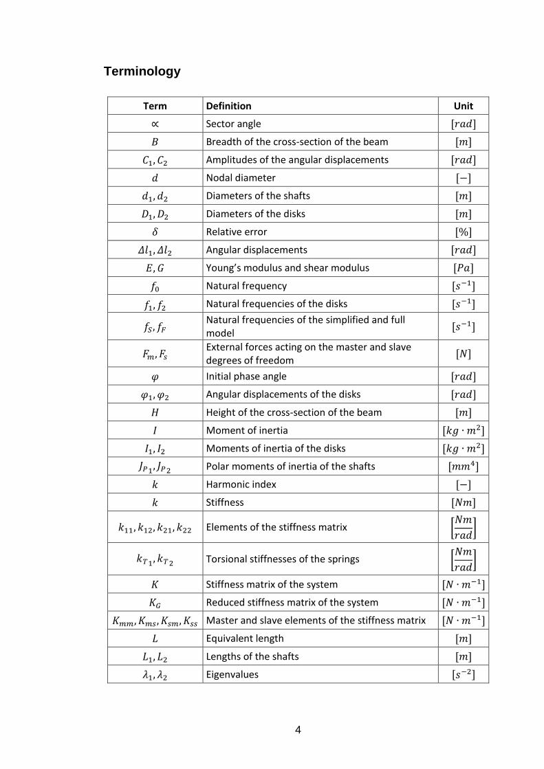
Terminology
Term Definition Unit
∝ Sector angle [𝑟𝑎𝑑]
𝐵 Breadth of the cross-section of the beam [𝑚]
𝐶1, 𝐶2 Amplitudes of the angular displacements [𝑟𝑎𝑑]
𝑑 Nodal diameter [−]
𝑑1, 𝑑2 Diameters of the shafts [𝑚]
𝐷1, 𝐷2 Diameters of the disks [𝑚]
𝛿 Relative error [%]
𝛥𝑙1, 𝛥𝑙2 Angular displacements [𝑟𝑎𝑑]
𝐸, 𝐺 Young’s modulus and shear modulus [𝑃𝑎]
𝑓0 Natural frequency [𝑠−1]
𝑓1, 𝑓2 Natural frequencies of the disks [𝑠−1]
𝑓𝑆 , 𝑓𝐹 Natural frequencies of the simplified and full model
[𝑠−1]
𝐹𝑚, 𝐹𝑠 External forces acting on the master and slave degrees of freedom
[𝑁]
𝜑 Initial phase angle [𝑟𝑎𝑑]
𝜑1, 𝜑2 Angular displacements of the disks [𝑟𝑎𝑑]
𝐻 Height of the cross-section of the beam [𝑚]
𝐼 Moment of inertia [𝑘𝑔 ∙ 𝑚2]
𝐼1, 𝐼2 Moments of inertia of the disks [𝑘𝑔 ∙ 𝑚2]
𝐽𝑃1, 𝐽𝑃2
Polar moments of inertia of the shafts [𝑚𝑚4]
𝑘 Harmonic index [−]
𝑘 Stiffness [𝑁𝑚]
𝑘11, 𝑘12, 𝑘21, 𝑘22 Elements of the stiffness matrix [𝑁𝑚
𝑟𝑎𝑑]
𝑘𝑇1, 𝑘𝑇2
Torsional stiffnesses of the springs [𝑁𝑚
𝑟𝑎𝑑]
𝐾 Stiffness matrix of the system [𝑁 ∙ 𝑚−1]
𝐾𝐺 Reduced stiffness matrix of the system [𝑁 ∙ 𝑚−1]
𝐾𝑚𝑚, 𝐾𝑚𝑠, 𝐾𝑠𝑚, 𝐾𝑠𝑠 Master and slave elements of the stiffness matrix [𝑁 ∙ 𝑚−1]
𝐿 Equivalent length [𝑚]
𝐿1, 𝐿2 Lengths of the shafts [𝑚]
𝜆1, 𝜆2 Eigenvalues [𝑠−2]
Page 5
5
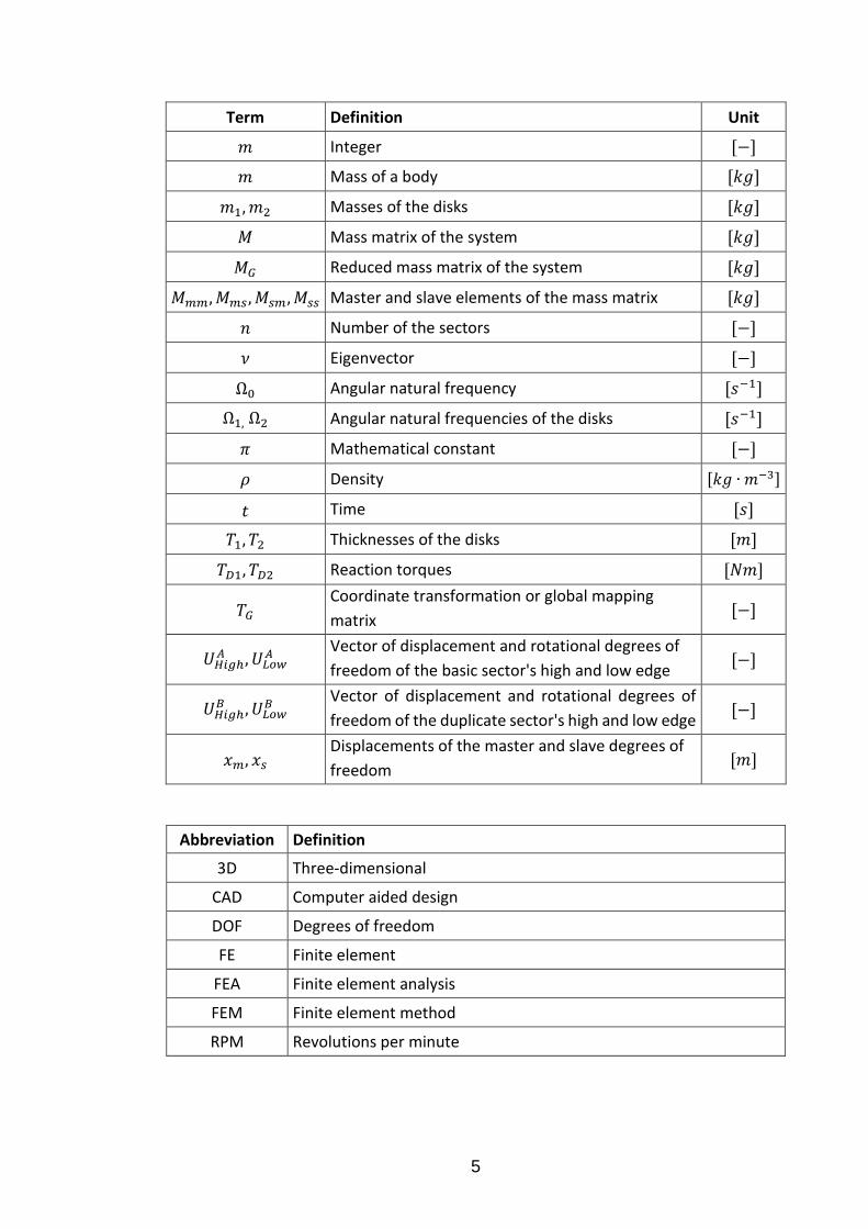
Term Definition Unit
𝑚 Integer [−]
𝑚 Mass of a body [𝑘𝑔]
𝑚1, 𝑚2 Masses of the disks [𝑘𝑔]
𝑀 Mass matrix of the system [𝑘𝑔]
𝑀𝐺 Reduced mass matrix of the system [𝑘𝑔]
𝑀𝑚𝑚, 𝑀𝑚𝑠 , 𝑀𝑠𝑚, 𝑀𝑠𝑠 Master and slave elements of the mass matrix [𝑘𝑔]
𝑛 Number of the sectors [−]
𝜈 Eigenvector [−]
Ω0 Angular natural frequency [𝑠−1]
Ω1, Ω2 Angular natural frequencies of the disks [𝑠−1]
𝜋 Mathematical constant [−]
𝜌 Density [𝑘𝑔 ∙ 𝑚−3]
𝑡 Time [𝑠]
𝑇1, 𝑇2 Thicknesses of the disks [𝑚]
𝑇𝐷1, 𝑇𝐷2 Reaction torques [𝑁𝑚]
𝑇𝐺 Coordinate transformation or global mapping
matrix [−]
𝑈𝐻𝑖𝑔ℎ𝐴 , 𝑈𝐿𝑜𝑤
𝐴 Vector of displacement and rotational degrees of
freedom of the basic sector's high and low edge [−]
𝑈𝐻𝑖𝑔ℎ𝐵 , 𝑈𝐿𝑜𝑤
𝐵 Vector of displacement and rotational degrees of
freedom of the duplicate sector's high and low edge [−]
𝑥𝑚, 𝑥𝑠 Displacements of the master and slave degrees of
freedom [𝑚]
Abbreviation Definition
3D Three-dimensional
CAD Computer aided design
DOF Degrees of freedom
FE Finite element
FEA Finite element analysis
FEM Finite element method
RPM Revolutions per minute
Page 6
6
1 Introduction
An integral part of the product’s design is performing simulations, which can
model a stress, deformations or dynamical behaviors of the product. One of the
most commonly used simulations is based on Finite element method FEM also
called Finite element analysis FEA. The basic principle of this method is dividing
a model into small pieces called finite elements. Each finite element is described
with a set of equations. Those equations are then assembled into larger set of
equations describing the whole model [1]. Static analysis of the simple model
consisting of a small number of finite elements can be quickly calculated on the
paper, however with more complicated models a number of finite elements and
thus, a number of equations increases. In that case, computers are involved.
Nowadays, models are larger and more complex and even using computers with
higher performance, calculations can last tens of hours. Right from the beginning
of the FEM analysis, engineers had to deal with limited computation resources.
Later, companies started to demand shorter time for the development of the prod-
ucts. Therefore, a need of methods dealing with large complex mechanical sys-
tems arose. The main question was how the model can be simplified so that it
will use less computational effort and simultaneously results would be precise
enough compared with a full model analysis results.
The aim of the thesis is to present four widely used model simplification methods
which can reduce computation effort in mechanical analysis. These methods are
Guyan static reduction method, Symmetry, Geometry simplification method and
Multibody system.
The thesis is divided into two parts. In the first part, simplification methods are
described along with their advantages, disadvantages and usage. The second
part demonstrates the functionality of methods on simple and understandable ex-
amples.
Page 7
7
2 Model simplification methods
During the last decades many simplification methods for reducing the computa-
tion time have been developed. In this chapter, four methods are presented.
These methods are Guyan static reduction method, Symmetry, Geometry simpli-
fication method and Multibody system. Each method has its own advantages and
disadvantages, and can be used in various cases.
2.1 Guyan static reduction method
As mentioned in the Introduction, large models can have several millions degrees
of freedom and analysing such models would take lots of time. The idea of Guyan
reduction method is that when a structure is excited some degrees of freedom
may have a more significant response than the others. By eliminating those de-
grees of freedom, which do not contribute on the model’s response, we can sig-
nificantly reduce the model. [1]
2.1.1 Definition
All degrees of freedom in the discrete model can be re-ordered as master de-
grees of freedom (retained) and slave degrees of freedom (discarded) so that the
system equation of motion can be written as
[𝑀𝑚𝑚 𝑀𝑚𝑠
𝑀𝑠𝑚 𝑀𝑠𝑠]
𝑥
𝑥 + [
𝐾𝑚𝑚 𝐾𝑚𝑠
𝐾𝑠𝑚 𝐾𝑠𝑠]
𝑥𝑚
𝑥𝑠 =
𝐹𝑚
𝐹𝑠 (1)
where m refers to master degrees of freedom and s indicates slave degrees of
freedom.
The Guyan approximation considers static solution in which neglects the inertia
effects [2] so that Eq. (1) condense to
[𝐾𝑚𝑚 𝐾𝑚𝑠
𝐾𝑠𝑚 𝐾𝑠𝑠]
𝑥𝑚
𝑥𝑠 =
𝐹𝑚
𝐹𝑠 (2)
After multiplication of matrices Eq. (2) is in the form
𝐾𝑚𝑚𝑥𝑚 + 𝐾𝑚𝑠𝑥𝑠 = 𝐹𝑚 (3)
𝐾𝑠𝑚𝑥𝑚 + 𝐾𝑠𝑠𝑥𝑠 = 𝐹𝑠 (4)
Page 8
8
Guyan (1965) assumed that external forces acting on the slave degrees of free-
dom are equal to zero, 𝐹𝑠 = 0, hence Eq. (4) leads to
𝐾𝑠𝑚𝑥𝑚 + 𝐾𝑠𝑠𝑥𝑠 = 𝐹𝑠 (5)
and after separation the 𝑥𝑠, it is received
𝑥𝑠 = −𝐾𝑠𝑠−1𝐾𝑠𝑚𝑥𝑚 (6)
Eq. (6) shows relations between master and slave displacements. Displacement
vector from the Eq. (6) can be written as
𝑥 = 𝑥𝑚
𝑥𝑠 = 𝑇𝐺𝑥𝑚 (7)
where 𝑇𝐺 is coordinate transformation matrix or global mapping matrix
𝑇𝐺 = [𝐼
−𝐾𝑠𝑠−1𝐾𝑠𝑚
] (8)
Then reduced stiffness matrix is
𝐾𝐺 = 𝑇𝐺𝑇𝐾𝑇𝐺 (9)
𝐾𝐺 = 𝐾𝑚𝑚 − 𝐾𝑚𝑠𝐾𝑠𝑠−1𝐾𝑠𝑚 (10)
And reduced mass matrix [3] is
𝑀𝐺 = 𝑇𝐺𝑇𝑀𝑇𝐺 (11)
𝑀𝐺 = 𝑀𝑚𝑚 − 𝐾𝑠𝑚𝑇 𝐾𝑠𝑠
−1𝑀𝑠𝑚 − 𝑀𝑚𝑠𝐾𝑠𝑠−1𝐾𝑠𝑚 + 𝐾𝑠𝑚
𝑇 𝐾𝑠𝑠−1𝑀𝑚𝑚𝐾𝑠𝑠
−1𝐾𝑠𝑚 (12)
Substituting Eq. (7) to the Eg. (1) and multiplying this expression by 𝑇𝐺 results in
a reduced-order system [1]
𝑇𝐺𝑇𝑀𝑇𝐺𝑥 + 𝑇𝐺
𝑇𝐾𝑇𝐺𝑥𝑚 = 𝑇𝐺𝑇𝐹 (13)
2.1.2 Numerical demonstration
Creating of the reduced mass and stiffness matrices is presented on the following
example. In Figure 1 3 DOF mass-stiffness system is shown. A mass 𝑚 = 1 𝑘𝑔
and a stiffness 𝑘 = 1 𝑁 ∙ 𝑚−1. The stiffness and mass matrices of the system can
be quickly obtained as
Page 9
9
𝐾 = [2 −1 0
−1 2 −10 −1 1
] , 𝑀 = [1 0 00 1 00 0 1
]
Figure 1. 3 DOF mass-stiffness system
Assuming the first and the third degree of freedom are selected as master de-
grees of freedom, rows and columns in the stiffness and mass matrices can be
reordered as
[𝐾𝑚𝑚 𝐾𝑚𝑠
𝐾𝑠𝑚 𝐾𝑠𝑠], [
𝑀𝑚𝑚 𝑀𝑚𝑠
𝑀𝑠𝑚 𝑀𝑠𝑠]
In our case, the mass matrix remains the same and for the reordering of the stiff-
ness matrix two steps can be done. Firstly, the 2nd row will change place with
the 3rd row, and secondly, the 2nd column will change a place with the 3rd col-
umn as shown below
[2 −1 0
−1 2 −10 −1 1
] → [2 −1 00 −1 1
−1 2 −1] → [
2 0 −10 1 −1
−1 −1 2]
From this can be extracted
𝐾𝑚𝑚 = [2 00 1
], 𝐾𝑠𝑠 = [2], 𝐾𝑚𝑠 = [−1−1
], 𝐾𝑠𝑚 = [−1 −1]
Then a reduced stiffness matrix is calculated according to the Eq. (10)
𝐾𝐺 = 𝐾𝑚𝑚 − 𝐾𝑚𝑠𝐾𝑠𝑠−1𝐾𝑠𝑚 = [
2 00 1
] − [−1−1
] [2]−1[−1 −1] = [1.5 −0.5
−0.5 0.5]
In the same way a reduced mass matrix can be calculated using Eq. (12).
Page 10
10
2.1.3 How to select master coordinates
The question is how the master degrees of freedom should be selected. Guyan
approximation neglects inertias associated with slave degrees of freedom, there-
fore master degrees of freedom are chosen where the inertia, damping and load
is high. [4]
2.1.4 Advantages and disadvantages
The main advantages of Guyan reduction method are that it is computationally
efficient and easy to implement. The method is also used in many commercial
FEA softwares including MSC-NASTRAN and ANSYS [5].
The main disadvantage of Guyan reduction method is that it neglects inertias
associated with the slave degrees of freedom. The method is unacceptable for
systems with high mass/stiffness ratios. The method is exact for static problems,
but for dynamic problems the accuracy is very low and depends on selection of
masters. Furthermore, with increasing natural frequencies, the error is increasing
as well, therefore this method is suitable only for calculating lower modes. [3], [5]
2.2 Symmetry
Many objects and structures have some kind of symmetry. Using the symmetry,
the system’s total number of degrees of freedom can be significantly reduced,
and therefore solution time to solve the problem. The use of symmetry does not
cause the loss of accuracy. Furthermore, a designer does not have to create full
model, but just its symmetrical part. [3], [6]
The symmetry can be used if the physical system exhibits symmetry in geometry,
loads, constraints and material properties. [7]
Types of symmetry (Figure 2)
Axial symmetry
Cyclic or rotational symmetry
Planar or reflective symmetry
Repetitive or translational symmetry [7]
Page 11
11
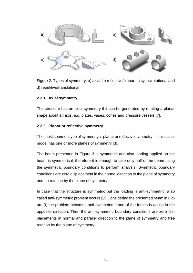
Figure 2. Types of symmetry: a) axial, b) reflective/planar, c) cyclic/rotational and
d) repetitive/translational
2.2.1 Axial symmetry
The structure has an axial symmetry if it can be generated by rotating a planar
shape about an axis, e.g. plates, vases, cones and pressure vessels [7].
2.2.2 Planar or reflective symmetry
The most common type of symmetry is planar or reflective symmetry. In this case,
model has one or more planes of symmetry [3].
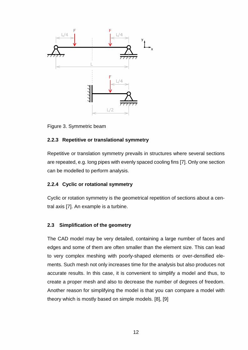
The beam presented in Figure 3 is symmetric and also loading applied on the
beam is symmetrical, therefore it is enough to take only half of the beam using
the symmetric boundary conditions to perform analysis. Symmetric boundary
conditions are zero displacement in the normal direction to the plane of symmetry
and no rotation by the plane of symmetry.
In case that the structure is symmetric but the loading is anti-symmetric, a so
called anti-symmetric problem occurs [8]. Considering the presented beam in Fig-
ure 3, the problem becomes anti-symmetric if one of the forces is acting in the
opposite direction. Then the anti-symmetric boundary conditions are zero dis-
placements in normal and parallel direction to the plane of symmetry and free
rotation by the plane of symmetry.
Page 12
12
Figure 3. Symmetric beam
2.2.3 Repetitive or translational symmetry
Repetitive or translation symmetry prevails in structures where several sections
are repeated, e.g. long pipes with evenly spaced cooling fins [7]. Only one section
can be modelled to perform analysis.
2.2.4 Cyclic or rotational symmetry
Cyclic or rotation symmetry is the geometrical repetition of sections about a cen-
tral axis [7]. An example is a turbine.
2.3 Simplification of the geometry
The CAD model may be very detailed, containing a large number of faces and
edges and some of them are often smaller than the element size. This can lead
to very complex meshing with poorly-shaped elements or over-densified ele-
ments. Such mesh not only increases time for the analysis but also produces not
accurate results. In this case, it is convenient to simplify a model and thus, to
create a proper mesh and also to decrease the number of degrees of freedom.
Another reason for simplifying the model is that you can compare a model with
theory which is mostly based on simple models. [8], [9]
Page 13
13
There are many simplification techniques [10], e.g. face clustering [11], edge dec-
imation based approach [12], decimation-cell transformation based technique
[13] and others. One of the most used techniques is removing details and features
such as chamfers, fillets, rounds and holes. The critical part is to determine
whether those features are important or not important for further analysis, in other
words, how much the model can be simplified to still obtain accurate results [14].
An example of a model with features, which can be removed or which cannot, is
illustrated in Figure 4. Considering modal analysis, this sheet metal model con-
tains several holes, projections and fillets which are very small and do not con-
tribute to its lowest mode shapes. Those features can be removed and then, the
simplified model is obtained including all necessary features which can affect the
analysis.
Figure 4. Left – full model, right – simplified model
Considering a complex model, trying to manually simplify such a model can be
very time-consuming. Therefore, many algorithms were created, which can ex-
tract CAD model information, remove unnecessary details and thus, make the
simplification process automatic.
2.4 Multibody system
The number of natural frequencies of the finite element model corresponds to its
number of degrees of freedom. The complex structures might have hundreds of
Page 14
14
thousands of degrees of freedom and thus, the same amount of natural frequen-
cies, however only ten or twenty modes could be enough to capture the overall
dynamic behavior of the structure [15].
The main goal of a multi-body model simplification is to create such a model
which can describe real systems behaviors using only the minimum of model en-
tities and ignoring the other features. This leads to dramatic reduction of the num-
ber of degrees of freedom. Basically, the problem is to know which features
should be neglected and which should sustain in a particular situation [16].
For example, a grinder mounted on the pedestal can be simplified as a vertical
beam vibrating in horizontal direction, with a mass at the top, shown in Figure 5.
It makes the grinder to be only 1 DOF system. Considering that the beam is fixed
to the floor, the bending stiffness of the beam can be calculated as [17]
𝑘 =3𝐸𝐼
𝐿3 (14)
where 𝐸 is Youngus Modulus, 𝐼 is a moment of inertia of the beam and 𝐿 is the
equivalent length of the beam.
Then the natural frequency of the beam is [17]
𝑓0 =1
2𝜋√
𝑘
𝑚 (15)
where 𝑘 is the beam stiffness and 𝑚 is a mass of the grinder.
Figure 5. Grinder on the pedestal on the left, 1 DOF model on the right (modified
figure [18])
Page 15
15
Although this example may seem to be simple and easy to implement, creating a
simplified system many times requires knowledge based on experience.
2.5 Summary
In the previous chapters, simplification methods were introduced. Table 1 sum-
marizes whether each method is applicable in the static and modal analysis or
not.
Guyan reduction
method Symmetry
Geometry simplification
Multibody system
Static analysis + +++ ++ + Modal analysis +++ ++ ++ ++
Table 1. Application of simplification methods in static and modal analysis
The most common approach in daily practice is to just remove unnecessary
grooves and fillets on a CAD model - Geometry simplification method. Also if
possible, it is recommended to use an advantage of symmetry. Guyan reduction
method is used in commercial FEA softwares including MSC-NASTRAN and AN-
SYS. Creation of multibody system highly depends on a particular study case.
All methods demand more or less of time for the preparation. An engineer has to
decide, firstly, if the simplification method is applicable for a particular case and
secondly, if a process of the model simplification does not consume more time
than the full model analysis itself.
Finally, mechanical simulations should be followed by practical measurements in
order to confirm reliability of both, measurements and simulations. This is espe-
cially true in the case when the model is simplified using any of the presented
simplification methods.
Page 16
16
3 Practical part
The main purpose of the practical part is to present several case studies which
can show the reliability of model simplification methods presented in the theoret-
ical part. The first study case is made as a multibody system. The second study
case deals with Guyan static reduction method. In the third study case an exam-
ple of a geometrical simplification is presented. In the fourth study case a cyclic
symmetry is used in order to simplify the model.
3.1 Disks
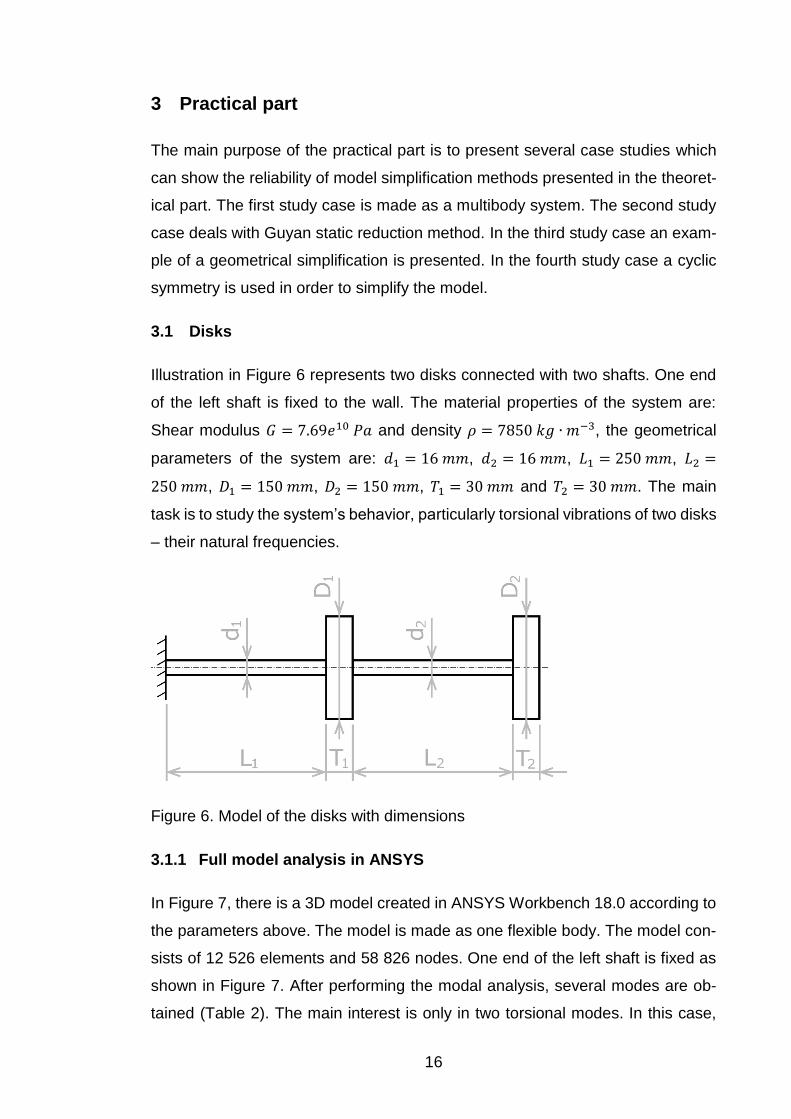
Illustration in Figure 6 represents two disks connected with two shafts. One end
of the left shaft is fixed to the wall. The material properties of the system are:
Shear modulus 𝐺 = 7.69𝑒10 𝑃𝑎 and density 𝜌 = 7850 𝑘𝑔 ∙ 𝑚−3, the geometrical
parameters of the system are: 𝑑1 = 16 𝑚𝑚, 𝑑2 = 16 𝑚𝑚, 𝐿1 = 250 𝑚𝑚, 𝐿2 =
250 𝑚𝑚, 𝐷1 = 150 𝑚𝑚, 𝐷2 = 150 𝑚𝑚, 𝑇1 = 30 𝑚𝑚 and 𝑇2 = 30 𝑚𝑚. The main
task is to study the system’s behavior, particularly torsional vibrations of two disks
– their natural frequencies.
Figure 6. Model of the disks with dimensions
3.1.1 Full model analysis in ANSYS
In Figure 7, there is a 3D model created in ANSYS Workbench 18.0 according to
the parameters above. The model is made as one flexible body. The model con-
sists of 12 526 elements and 58 826 nodes. One end of the left shaft is fixed as
shown in Figure 7. After performing the modal analysis, several modes are ob-
tained (Table 2). The main interest is only in two torsional modes. In this case,
Page 17
17
torsional modes are 3 and 6 with natural frequencies 40.192 Hz and 105 Hz re-
spectively (torsional modes can be recognized from total deformation animations
in ANSYS).
Figure 7. Full model – fixed support
Mode 1 2 3 4 5 6 7
Frequency [Hz] 8.0638 8.0643 40.192 53.311 53.319 105 186.170
Table 2. Modes with corresponding frequencies
3.1.2 Simplified multibody model
Figure 8 illustrates a simplified multibody model consisting of two inertias and two
torsional springs. Inertias of springs are neglected. The system has the following
parameters: torsional stiffness of the 1st spring 𝑘𝑇1, torsional stiffness of the 2nd
spring 𝑘𝑇2, the 1st moment of inertia 𝐼1 and the 2nd moment of inertia 𝐼2. The
system has 2 DOFs – rotations about x-axis.
Figure 8. Simplified model
Page 18
18
Pre-calculations
Firstly, simplified multibody model parameters are obtained from the dimensions
of the full model. Beginning with masses of the disks
𝑚1 = 𝜌 ∙ 𝜋 (𝐷1
2)
2
∙ 𝑇1 = 7850 ∙ 𝜋 (0.15
2)
2
∙ 0.03 = 4.16 𝑘𝑔 (16)
𝑚2 = 𝜌 ∙ 𝜋 (𝐷2
2)
2
∙ 𝑇2 = 7850 ∙ 𝜋 (0.15
2)
2
∙ 0.03 = 4.16 𝑘𝑔 (17)
moments of inertia of the disks can be calculated as
𝐼1 =1
2𝑚1 (
𝐷1
2)
2
=1
2∙ 4.16 ∙ (
0.15
2)
2
= 0.0117 𝑘𝑔 ∙ 𝑚2 (18)
𝐼2 =1
2𝑚2 (
𝐷2
2)
2
=1
2∙ 4.16 ∙ (
0.15
2)
2
= 0.0117 𝑘𝑔 ∙ 𝑚2 (19)
Polar moments of inertia of the shafts are
𝐽𝑃1= 𝜋
𝑑14
32= 𝜋
0.0164
32= 6.434e−9 𝑚𝑚4 (20)
𝐽𝑃2= 𝜋
𝑑24
32= 𝜋
0.0164
32= 6.434e−9 𝑚𝑚4 (21)
From which can be calculated torsional stiffness of the springs
𝑘𝑇1=
𝐺 ∙ 𝐽𝑃1
𝐿1=
7.69𝑒10 ∙ 6.434e−9
0.25= 1979.69
𝑁 ∙ 𝑚
𝑟𝑎𝑑(22)
𝑘𝑇2=
𝐺 ∙ 𝐽𝑃2
𝐿2=
7.69𝑒10 ∙ 6.434e−9
0.25= 1979.69
𝑁 ∙ 𝑚
𝑟𝑎𝑑(23)
Calculations
Equations of motion can be derived using Newton’s force method. Figure 9 shows
the free body diagram of the system.
Page 19
19
Figure 9. Free body diagram
Equations of motion are
𝐼1 ∙ 𝜑1 = ∑ 𝑇1𝑖 = − 𝑇𝐷1 + 𝑇𝐷2 (24)
𝐼2 ∙ 𝜑2 = ∑ 𝑇2𝑖 = − 𝑇𝐷2 (25)
Reaction torques are
𝑇𝐷1 = 𝑘𝑇1𝛥𝑙1 = 𝑘𝑇1
𝜑1 (26)
𝑇𝐷2 = 𝑘𝑇2𝛥𝑙2 = 𝑘𝑇2
(𝜑2 − 𝜑1) (27)
where 𝛥𝑙1 and 𝛥𝑙2 are angular displacements.
Introducing Eq. (26) and (27) into Eq. (24) and (25) produces
𝐼1 ∙ 𝜑1 + 𝑘𝑇1𝜑1 − 𝑘𝑇2
(𝜑2 − 𝜑1) = 0 (28)
𝐼2 ∙ 𝜑2 + 𝑘𝑇2(𝜑2 − 𝜑1) = 0 (29)
and after reordering
𝐼1 ∙ 𝜑1 + (𝑘𝑇1+ 𝑘𝑇2
)𝜑1 − 𝑘𝑇2𝜑2 = 0 (30)
𝐼2 ∙ 𝜑2 − 𝑘𝑇2𝜑1 + 𝑘𝑇2
𝜑2 = 0 (31)
Eq. (30) and Eq. (31) can be written as
[𝐼1 00 𝐼2
] ∙ 𝜑1
𝜑2 + [
𝑘𝑇1+ 𝑘𝑇2
−𝑘𝑇2
−𝑘𝑇2𝑘𝑇2
] ∙ 𝜑1
𝜑2 =
00
(32)
Page 20
20
Assuming the solution as
𝜑1(𝑡) = 𝐶1 ∙ sin(𝛺0 ∙ 𝑡 + 𝜑) (33)
𝜑2(𝑡) = 𝐶2 ∙ sin(𝛺0 ∙ 𝑡 + 𝜑) (34)
and
1(𝑡) = −𝐶1 ∙ 𝛺02 ∙ sin(𝛺0 ∙ 𝑡 + 𝜑) (35)
2(𝑡) = −𝐶2 ∙ 𝛺02 ∙ sin(𝛺0 ∙ 𝑡 + 𝜑) (36)
where 𝛺0 is a natural frequency and 𝜑 is an initial phase angle.
And substituting solution into Eq. (30) and Eq. (31) is obtained
(𝑘11 − 𝜆 ∙ 𝐼1) ∙ 𝐶1 + 𝑘12𝐶2 = 0 (37)
𝑘21𝐶1 + (𝑘22 − 𝜆 ∙ 𝐼2) ∙ 𝐶2 = 0 (38)
which can be written as
(𝐾 − 𝜆 ∙ 𝑀) ∙ 𝑣 = 0 (39)
System of equations has a trivial solution. Searching for non-trivial solution 𝐶1 ≠
0, 𝐶2 ≠ 0, determinant of the expression in brackets has to be equal to zero
|𝐾 − 𝜆 ∙ 𝑀| = |𝑘11 − 𝜆 ∙ 𝐼1 𝑘12
𝑘21 𝑘22 − 𝜆 ∙ 𝐼2| =
= 𝐼1𝐼2𝜆2 − (𝑘11 ∙ 𝐼2 + 𝑘22 ∙ 𝐼1) ∙ 𝜆 + 𝑘11 ∙ 𝑘22 − 𝑘21 ∙ 𝑘12 = 0
This is the quadratic equation with the eigenvalue 𝜆 as an unknown parameter.
After inserting calculated values the quadratic equation results into
𝜆1 = 64604.9 𝑠−2 Ω1 = √𝜆1 = 254.1749 𝑠−1 𝑓1 =Ω1
2𝜋= 40.4532 𝐻𝑧 (41)
𝜆2 = 442808.45 𝑠−2 Ω2 = √𝜆2 = 665.4385 𝑠−1 𝑓2 =Ω2
2𝜋= 105.9078 𝐻𝑧 (42)
In order to get results and make changes quickly, all equations from this section
were implemented in MATLAB code.
(40)
Page 21
21
3.1.3 Results
Natural frequencies of simplified and full model and a relative error are written in
Table 3. The relative error 𝛿 in percents is calculated using formula
𝛿 =𝑓𝑆 − 𝑓𝐹
𝑓𝐹∙ 100 (43)
where 𝑓𝐹 is a natural frequency of the full model and 𝑓𝑆 is a natural frequency of
the simplified model.
Observing natural frequencies, it can be seen that the natural frequency of the
simplified model is higher than the frequency of the full model. A relative error for
the first mode is 0.6 % and for the second mode is 0.9 % which is a very small
error.
Natural frequencies [Hz]
Full Simplified delta [%]
Mode 1 40.1920 40.4532 0.6
Mode 2 105 105.9078 0.9
Table 3. Comparison of the natural frequencies
Considering several modifications of the model when the disks’ diameters 𝐷1 =
𝐷2 = 𝐷 are equally changing and other dimensions remain the same (Figure 10),
it can be observed how the ratio between the shaft diameter 𝑑 and disk diame-
ter 𝐷 affects results. Figure 11 shows the relation between a relative error and a
shaft/disk diameter ratio.
Figure 10. Changing of the shaft/disk diameter ratio
Page 22
22
Figure 11. Relation between a relative error and a shaft/disk diameter ratio
3.1.4 Discussion
In this case, it can be concluded that the results obtained from the simplified
model are accurate. Because of using different software for calculating the full
and simplified model, the time for solving the analysis was not provided. Never-
theless, the solution time can be presented as the number of degrees of freedom
entering the analysis. Comparing the full model with thousands of DOFs and the
simplified model with only two DOFs, in can be concluded that the solution time
was significantly reduced. However, the solution time does not include time for
the model’s preparation. In this case, creating and analyzing of the simplified
model and analyzing of the full model were both quick procedures. Considering
a more complex structure, a simplification process can take a lot of time (as men-
tioned in Chapter 2.5), therefore, an engineer has to consider which option is the
best for the particular case, if to analyze the full model or to make the simplifica-
tion.
The advantage of a simple model is that it is easy to perform a sensitivity analysis
and study how sensitive the system is for certain parameter changes. In this case
was examined how the changing of the model dimensions affects results. It has
to be noted that the inertias of the shafts were neglected due to the big difference
between the diameter of the disk and shaft. If both diameters are close to each
other (d/D increases to 0.5 as shown in Figure 11), inertias of the shafts cannot
be neglected.
0
2
4
6
8
10
12
14
16
0 0,1 0,2 0,3 0,4 0,5
Rel
ativ
e er
ror
[%]
d/D
Mode 1 Mode 2
Page 23
23
3.2 Beam
A cantilever beam is shown in Figure 12. One end of the beam is fixed. The ge-
ometrical parameters of the beam are 𝐿 = 200 𝑚𝑚, 𝐻 = 20 𝑚𝑚 and 𝐵 = 20 𝑚𝑚.
The material properties of the beam are Elastic modulus 𝐸 = 210000 𝑀𝑃𝑎 and
density 𝜌 = 7850 𝑘𝑔 ∙ 𝑚−3.
Figure 12. Cantilever beam
MATLAB code developed and provided by Dr. Jussi Sopanen is used to create
the finite element model of the beam, and perform full model analysis, Guyan
reduction method and simplified model analysis. [19]
The FE model of the beam in Figure 13 consists of 8 elements and 9 nodes. Each
node has three DOFs: translation in x-axis, translation in y-axis, and rotation in x-
y plane. The full model has 27 DOFs. The node no. 1 is fully constrained. The
natural frequencies for the first three modes of the model are 41.5807 Hz,
249.3972 Hz, and 649.6355 Hz respectively. The mode shapes are shown in
Figure 14.
Figure 13. Finite element model of the cantilever beam
The reduced model is created using Guyan reduction method (the procedure is
explained in Chapter 2.1.2) by selecting master nodes 4, 6 and 9. Each node has
3 DOFs, therefore the reduced model has 9 DOFs. The calculated natural fre-
quencies of the reduced model are 41.5927 Hz, 250.3926 Hz and 656.6683 Hz.
Page 24
24
Figure 14. Mode shapes of the cantilever beam
Let us see how the natural frequencies change using different master nodes. Ta-
ble 4 describes several variations of selected master nodes and corresponding
natural frequencies of the first three modes.
Master nodes 2, 9 4, 8 5, 8 2, 5, 9 4, 6, 8 4, 6, 9 5, 6, 7 Full
Mode 1 41,647 41,601 41,591 41,612 41,586 41,593 41,632 41,581
Mode 2 273,202 253,639 253,013 251,351 250,640 250,393 258,325 249,397
Mode 3 670,090 661,628 657,596 664,355 653,076 656,668 659,522 649,636
Table 4. Selected master nodes and corresponding natural frequencies
3.2.1 Results
Using Guyan static reduction method it can be seen from Table 4 that the se-
lected master nodes 4, 6, 8 give the closest values to the full system’s 1st and
3rd natural frequencies, and master nodes 4, 6, 9 to the 2nd natural frequency. It
can also be seen that the natural frequencies of the simplified models are all
higher than the natural frequencies of the full model. This is because of Guyan
reduction which makes the stiffness of the beam higher and mass of the beam
lower.
Focusing on the 1st mode, it can be observed that all frequencies using different
master nodes are very close to the full system frequency. It means that all nodes
Page 25
25
(except the fixed node no. 1) participate in the 1st mode, so for the 1st mode
frequency it does not matter that much which or how many nodes are set as
master nodes. In the 2nd mode, the calculated frequencies using different master
nodes, are also close to the full system’s frequency. However, frequencies in the
3rd mode differ a lot using different master nodes. Generally, with higher modes
the relative error is increasing.
3.2.2 Discussion
A simple example of the cantilever beam showed that using Guyan reduction
method can significantly reduce the analysis time and provide accurate results,
however selecting master degrees of freedom is crucial to obtain precise results.
Therefore, the question: How to correctly select master degrees of freedom? has
to be examined. The basic approach is to imagine a complex structure as a sim-
ple structure and then to observe how it acts. This may help to identify which parts
of the complex structure contribute in certain modes.
From Table 4 it can be seen that choosing three master nodes yields to more
precise results than choosing two master nodes, in other words, the more master
nodes, the higher precision. However, comparing natural frequencies for all
modes when master nodes are selected in the first case as 5, 8 and in the second
case as 5, 6, 7, can be concluded that choosing more master nodes does not
guarantee better results. This has to be also taken into account when selecting
master degrees of freedom.
3.3 Simplification of the geometry
In this section, three examples are presented (Figure 15) to validate how the sim-
plification of the geometry affects a static analysis. These examples were se-
lected because of the variety of geometrical details and boundary conditions.
Page 26
26
Figure 15. Case A, B and C (from the left to the right)
3.3.1 Models preparation
Figure 16 shows the boundary conditions BC applied on the full models (the same
BC are applied on simplified models). Figure 17 presents the models after sim-
plification. The following paragraphs describe how the models are simplified and
what boundary conditions are used.
Case A – All grooves on the left and right side of the model are eliminated. A
small hole going through the walls is suppressed and all small radiuses are re-
moved. Only bigger radiuses which are considered as critical places are kept
(Figure 17). The bottom of the model is fixed and the force was applied in the
vertical direction on the upper face (Figure 16).
Case B – In this case, only small radiuses are removed (Figure 17). Constraints
are applied on the holes where the part will be mounted with bolts to the wall. The
force is applied on the horizontal desk in the normal direction (Figure 16).
Case C – Straight stripes on the pedal are removed and all small radiuses are
eliminated (Figure 17). The hole is fully constraint and the force is applied on the
stripes in the normal direction to their faces (Figure 16).
For both models - full and simplified - such a mesh was generated which corre-
sponds to the model’s shape and geometrical details. This guarantees obtaining
precise results from the static analysis.
After an execution of a finite element analysis, the results between the original
and the simplified model are compared, namely equivalent stress, total defor-
mation and solution time.
Page 27
27
Figure 16. Boundary conditions – a) Case A, b) Case B, and c) Case C
Figure 17. Simplified models
Page 28
28
3.3.2 Results
Figures 18, 19 and 20 represent the results from the static analysis of the finite
element models of the three studied parts before and after removing details. The
results are summarized in Tables 5, 6 and 7. The left side of Figures 18, 19 and
20 shows the equivalent stress and the total displacement of the full model. The
right side of Figure 18, 19 and 20 shows the equivalent stress and the total dis-
placement of the simplified model.
Figure 18. Stress and deformation results for the full and simplified model – Case
A
CASE A Full model Simplified model Percentage [%]
Max Stress [MPa] 26.697 25.698 3.74
Max Displacement [mm] 4.62 ∙ 10−3 4.57 ∙ 10−3 0.89
Solution time [sec] 28 18 35.71
Table 5. Comparison of stress and deformation results – Case A
For Case A, the computation time saved by simplification of the model is 36%.
The equivalent stress error is 3.74% and the error related to the displacement is
0.89%.
Page 29
29
Figure 19. Stress and deformation results for the full and simplified model - Case
B
CASE B Full model Simplified model Percentage [%]
Max Stress [MPa] 53.299 55.549 4.22
Max Displacement [mm] 4.8 ∙ 10−2 5.11 ∙ 10−2 6.47
Solution time [sec] 38 29 23.68
Table 6 – Comparison of stress and deformation results – Case B
For Case B, the saved computation time is 24%, the equivalent stress is 4.22%,
whereas the displacement error reaches the value 6.47%.
Page 30
30
Figure 20. Stress and deformation results for the full and simplified model – Case
C
CASE C Full model Simplified model Percentage [%]
Max Stress [MPa] 82.659 82.814 0.19
Max Displacement [mm] 2.98 ∙ 10−1 2.99 ∙ 10−1 0.61
Solution time [sec] 30 19 36.67
Table 7. Comparison of stress and deformation results – Case C
For Case C, the saved computation time is 37%. The equivalent stress error is
0.19% and the displacement error is 0.61%.
Comparing the results of all three cases, it can be seen that for Case C, the sim-
plification brought the highest saved computation time with a minimum error. It
can be concluded that removing details on Case C did not affect the results of
static analysis. Acceptance of errors of Case A and B has to be decided according
to the model’s purpose and function. Another noticeable point is that the simplifi-
cation of the model causes increasing or decreasing of equivalent stress and the
total deformation in a particular case.
Page 31
31
3.3.3 Discussion
The whole process of simplification of the models was made manually using a 3D
modelling software. Details such as small fillets, holes and grooves were consid-
ered to be removed from the full model, whereas several fillets and features were
kept because they could significantly affect analysis results. This can be seen on
Case A, where the maximum equivalent stress was found on one of the bigger
fillets. In Case B, only small radiuses were removed. This caused around 4%
stress error. Case C shows that changes on the geometry (e.g. removing stripes)
made far from the critical place, do not affect the analysis results.
Manual removing of the details can take a long time, therefore it is convenient to
use an algorithm as mentioned in Chapter 2.3, which makes the process auto-
matic. However, it still has to be considered if the simplification and analysis of
the model does not consume more time than a direct analysis of the full model.
3.4 Impeller
In this section a simplification using a cyclic symmetry is presented on an exam-
ple of impeller (Figure 21). Firstly, the static analysis is performed on a full model
and on one segment from the impeller. Secondly, the modal analysis is performed
on the full model and on the segment. Analyses are made in ANSYS Workbench
18.0, the process of applying the cyclic symmetry in ANSYS is explained in the
following section.
Figure 21. Models of the full impeller and its one segment
Page 32
32
3.4.1 Modal cyclic symmetry in ANSYS
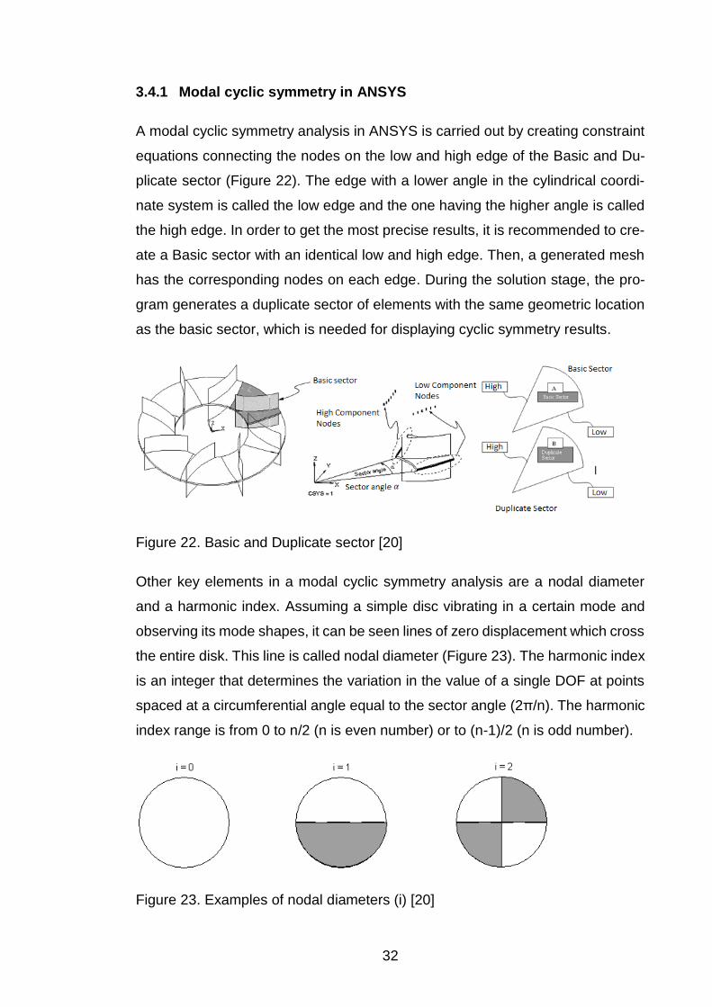
A modal cyclic symmetry analysis in ANSYS is carried out by creating constraint
equations connecting the nodes on the low and high edge of the Basic and Du-
plicate sector (Figure 22). The edge with a lower angle in the cylindrical coordi-
nate system is called the low edge and the one having the higher angle is called
the high edge. In order to get the most precise results, it is recommended to cre-
ate a Basic sector with an identical low and high edge. Then, a generated mesh
has the corresponding nodes on each edge. During the solution stage, the pro-
gram generates a duplicate sector of elements with the same geometric location
as the basic sector, which is needed for displaying cyclic symmetry results.
Figure 22. Basic and Duplicate sector [20]
Other key elements in a modal cyclic symmetry analysis are a nodal diameter
and a harmonic index. Assuming a simple disc vibrating in a certain mode and
observing its mode shapes, it can be seen lines of zero displacement which cross
the entire disk. This line is called nodal diameter (Figure 23). The harmonic index
is an integer that determines the variation in the value of a single DOF at points
spaced at a circumferential angle equal to the sector angle (2π/n). The harmonic
index range is from 0 to n/2 (n is even number) or to (n-1)/2 (n is odd number).
Figure 23. Examples of nodal diameters (i) [20]
Page 33
33
The nodal diameter is the same as the harmonic index in only some cases. The
relationship between the harmonic index 𝑘 and the nodal diameter 𝑑 for a model
consisting of 𝑛 sectors is:
𝑑 = 𝑚 ∙ 𝑛 ± 𝑘, 𝑚 = 0, 1, 2 …
Finally, the constraint equations for edge-component nodes are
𝑈𝐻𝑖𝑔ℎ
𝐴
𝑈𝐻𝑖𝑔ℎ𝐵 = [
𝑐𝑜𝑠𝑘𝛼 𝑠𝑖𝑛𝑘𝛼𝑠𝑖𝑛𝑘𝛼 𝑐𝑜𝑠𝑘𝛼
] 𝑈𝐿𝑜𝑤
𝐴
𝑈𝐿𝑜𝑤𝐵
where 𝑘 is harmonic index, 𝛼 is sector angle and 𝑈 is a vector of displacement
and rotational degrees of freedom. The equation is a function of harmonic in-
dex, and generates different sets of constraint equations for each harmonic in-
dex. [20]
3.4.2 Full model
A CAD model of the impeller was created in Solidworks. A base of the impeller is
formed from a disk with a hole in the middle. The impeller has five blades con-
nected with the ring, which are equally placed 72° from each other about the
central axis. A generated mesh is made from tetrahedrons, the mesh contains
106 233 nodes and the number of elements is 60 855. Boundary conditions for a
static analysis are displayed in Figure 24. A hole in the middle of the impeller is
fully constrained. A rotational velocity 942 rad/s (9 000 RPM) is about z-axis of
Global Coordinate System, which is located to the Centre of Gravity of the impel-
ler. The results to be observed in the static analysis are equivalent stress and
total deformation.
Figure 24. Full model - mesh (left) and boundary conditions (right)
Page 34
34
As a boundary condition for the modal analysis the fixed support of the hole is
chosen. The results to be observed in the modal analysis are natural frequencies
and mode shapes. The main focus is on the first 6 modes.
3.4.3 One segment
The impeller contains a circular pattern of 5 sections. One section can be ex-
tracted to perform the modal analysis. A cut section, displayed in Figure 25, con-
tains one blade, the angle between two cutting planes is 360/5=72°. Before cre-
ating a mesh, a new cylindrical coordinate system was created with x-axis in the
radial direction, y-axis presenting the angle coordinate and z-axis in the axial di-
rection. As explained in Chapter 3.4.1, a cyclic symmetry feature with its low and
high boundary conditions has to be set up. A low boundary condition was selected
on the right face and a high boundary condition was selected on the left face of
the section according to the growing angle coordinate (Figure 25).
Fig. 25 – High and low edges
A mesh was created from tetrahedrons, the number of nodes in the mesh is 22
562 and the number of elements is 12 621 which is approximately 5 times less
than in the full model (Figure 26).
Page 35
35
Figure 26. One segment - mesh (left) and boundary conditions (right)
Similarly, as in the full model, the boundary conditions for the static analysis ap-
plied on one section are fixed support for the inner surface of the hole and a
rotational velocity 942 rad/s acting along z-axis of the cylindrical coordinate sys-
tem (Figure 26). The results to be observed in the static analysis are equivalent
stress and total deformation. A boundary condition in the modal analysis is a fixed
support applied on the inner surface of the hole. The results to be observed are
natural frequencies and mode shapes. The main interest is on the first 6 modes.
In our case, a full model has 5 repeating segments, therefore the range of the
harmonic indices is from 0 to (5-1)/2 = 2. Together it is 3 harmonic indices. How-
ever, setting up 6 modes in ANSYS analysis settings using a cyclic symmetry
would result into a number of modes which is equal to a number of searched
modes times a number of harmonic indices, in our case, it is 6x3=18 modes. In
order to obtain just 6 modes from the analysis, a needed number of searched
modes is 2.
3.4.4 Results – static analysis
Figure 27 shows the results from the static analysis – the equivalent stress and
total deformation of the full model (on the left) and of one segment from the im-
peller (on the right). Even though just one segment of the impeller was analysed,
ANSYS displays the whole model by multiplying the results of one segment.
Page 36
36
Figure 27. Stress and deformation results for the full model and one segment
The values of the maximum equivalent stress and the total deformation are writ-
ten in Table 8. The equivalent stress error is 0.88% and the error related to the
displacement is 0.1%. The solution time saved using a cyclic symmetry is 50%.
Full model One section Percentage [%]
Max Stress [MPa] 140.61 139.37 0.88
Max Displacement [mm] 7.02 ∙ 10−2 7.02 ∙ 10−2 0.10
Solution time [sec] 22 11 50.00
Table 8. Comparison of stress and deformation results
3.4.5 Results – modal analysis
Beginning with the modal analysis of one segment, ANSYS provides results in a
form of harmonic indices and its corresponding frequencies as shown in Table 9.
Page 37
37
Table 9. Results from the modal cyclic symmetry analysis
Agreed with the calculation before, there are 3 harmonic indices. The mode
shapes corresponding to the natural frequencies are shown in Figure 28.
Figure 28. Mode shapes – harmonic index 0, 1 and 2 (from the top to the bottom)
Mode Harmonic index Frequency [Hz]
1 0 1198.9
2 0 1235.9
1 1 647.41
2 1 647.41
1 2 1009.9
2 2 1009.9
Page 38
38
The mode shapes of the harmonic index 0 represent the so called umbrella shape
where the middle of the impeller is fixed and the rest is moving in the same direc-
tion up and down. The mode shapes of the harmonic index 1 represent a travel-
ling wave passing through the circumference. The modes shapes are similar with
90° angle shift, their corresponding natural frequencies are the same. Mode
shapes of the harmonic index 2 show two zero displacement planes perpendicu-
lar to each other. The mode shapes of the full model are not displayed because
they are similar to the mode shapes of one segment.
Natural frequencies of one segment are sorted from the least to the highest fre-
quency, and compared with natural frequencies of the full model in Table 10. A
maximum relative error between natural frequencies is approximately 0.2%.
Mode Full model
frequency [Hz] One segment
frequency [Hz]
1 647.94 647.41
2 648.72 647.41
3 1009.8 1009.9
4 1009.8 1009.9
5 1199.2 1198.9
6 1236.2 1235.9
Table 10. Comparison of the natural frequencies of the full model and one seg-
ment
The solution time for analysing of the full model is 40 seconds and the analysis
using cyclic symmetry takes 32 seconds, which makes a saving time 20%.
3.4.6 Discussion
The results from the static analysis state that the relative stress error is under one
percent. The difference between the results of the full model and one section of
the model can be caused due to a different mesh on each model. The advantage
of the cyclic symmetry is that even a denser mesh can be generated on one seg-
ment in order to receive more precise results, and still it consumes less time for
solving the analysis than analysing of the full model.
Page 39
39
In this case, creating a cyclic symmetry saved 50% of the solution time in the
static analysis. This work presented just one example, still it can be assumed that
if a part would have had more cyclic segments, the saved solution time would
significantly increase.
Setting up a cyclic symmetry in ANSYS is not difficult. However, it is necessary
to calculate the number of harmonic indices before starting the analysis in order
to set up the right number of modes as explained in Chapter 3.4.3.
In this work, the main interest was in the first 6 modes and the relative error be-
tween the natural frequencies turned out to be very small. Nevertheless, calcu-
lating more modes is needed to verify if cyclic symmetry in ANSYS provides ac-
ceptable results for higher frequencies.
Page 40
40
4 Conclusion
The main goal of the thesis was to present four simplification methods for model
reduction in mechanical analysis, and demonstrate their applicability on simple
examples. For each example analysis of its full model and simplified model was
performed. The results from both analyses were compared in order to verify the
functionality of the methods.
In the first example, a multibody system was created based on the model of two
disks connected with shafts. A relative error of natural frequencies for two modes
did not reach 1%. It was also shown that if there is a small difference between
the size of the disk diameter and the shaft diameter, the relative error significantly
increases.
Another example of the cantilever beam demonstrated application of Guyan re-
duction method. Different master nodes were selected in order to observe how
much selected nodes contribute on particular mode shapes. From the results it
was visible that Guyan reduction method is beneficial in the modal analysis, how-
ever it highly depends which nodes are selected as master nodes.
Simplification of geometry was studied on three examples – Case A, B and C.
The static analyses of models were performed. By removing unnecessary details
from the models saving of the computation time up to 37% was achieved. Re-
moving details had different impact on the results in each case. It was pointed
out that several details cannot be removed, because they are a part of critical
places where the maximum stress is.
In the last example, cyclic symmetry in ANSYS was applied on the model of the
impeller. The solution time in the static analysis was reduced to 50% and in the
modal analysis to 20%. It was shown that cyclic symmetry in ANSYS is easy to
implement. The obtained results were precise enough reaching only the relative
stress error 0.9% in the static analysis and the relative frequency error 0.2% in
the modal analysis.
The thesis showed that applications of presented simplification methods were
beneficial for reducing computational effort in mechanical analysis for the given
Page 41
41
cases. In the future work, the main interest would lay on discovering more simpli-
fication methods followed with more complex examples.
Page 42
42
Figures and tables
Figure 1. 3 DOF mass-stiffness system .............................................................. 9
Figure 2. Types of symmetry: a) axial, b) reflective/planar, c) cyclic/rotational and
d) repetitive/translational ................................................................................... 11
Figure 3. Symmetric beam ................................................................................ 12
Figure 4. Left – full model, right – simplified model ........................................... 13
Figure 5. Grinder on the pedestal on the left, 1 DOF model on the right (modified
figure [18]) ......................................................................................................... 14
Figure 6. Model of the disks with dimensions ................................................... 16
Figure 7. Full model – fixed support .................................................................. 17
Figure 8. Simplified model ................................................................................ 17
Figure 9. Free body diagram ............................................................................. 19
Figure 10. Changing of the shaft/disk diameter ratio ......................................... 21
Figure 11. Relation between a relative error and a shaft/disk diameter ratio .... 22
Figure 12. Cantilever beam ............................................................................... 23
Figure 13. Finite element model of the cantilever beam ................................... 23
Figure 14. Mode shapes of the cantilever beam ............................................... 24
Figure 15. Case A, B and C (from the left to the right) ...................................... 26
Figure 16. Boundary conditions – a) Case A, b) Case B, and c) Case C .......... 27
Figure 17. Simplified models ............................................................................. 27
Figure 18. Stress and deformation results for the full and simplified model – Case
A ....................................................................................................................... 28
Figure 19. Stress and deformation results for the full and simplified model - Case
B ....................................................................................................................... 29
Figure 20. Stress and deformation results for the full and simplified model – Case
C ....................................................................................................................... 30
Figure 21. Models of the full impeller and its one segment ............................... 31
Figure 22. Basic and Duplicate sector [20] ....................................................... 32
Figure 23. Examples of nodal diameters (i) [20]................................................ 32
Figure 24. Full model - mesh (left) and boundary conditions (right) .................. 33
Fig. 25 – High and low edges............................................................................ 34
Figure 26. One segment - mesh (left) and boundary conditions (right) ............. 35
Figure 27. Stress and deformation results for the full model and one segment 36
Page 43
43
Figure 28. Mode shapes – harmonic index 0, 1 and 2 (from the top to the bottom)
.......................................................................................................................... 37
Table 1. Application of simplification methods in static and modal analysis ...... 15
Table 2. Modes with corresponding frequencies ............................................... 17
Table 3. Comparison of the natural frequencies ............................................... 21
Table 4. Selected master nodes and corresponding natural frequencies ......... 24
Table 5. Comparison of stress and deformation results – Case A .................... 28
Table 6 – Comparison of stress and deformation results – Case B .................. 29
Table 7. Comparison of stress and deformation results – Case C .................... 30
Table 8. Comparison of stress and deformation results .................................... 36
Table 9. Results from the modal cyclic symmetry analysis ............................... 37
Table 10. Comparison of the natural frequencies of the full model and one
segment ............................................................................................................ 38
References
1. INMAN, D. J. Engineering vibration. Fourth edition. Boston: Pearson, 2014. ISBN 978-0132871693.
2. Chung, Y. T. Model Reduction and Model Correlation Using MSC/NAS-TRAN. MSC 1995 World Users’ Conf. Proc., 1995.
3. QU, Zu-Qing. Model order reduction techniques. ISBN 18-523-3807-5, pp. 47-49.
4. Sopanen, J. 2017WK46_Lecture_10_FEM_Model_Reduction [Lecture]. Lap-peenranta, Lappeenranta University of Technology, 2017
5. Flanigan, C. C. Model Reduction Using Guyan IRS and Dynamic Methods. SPIE International Society for Optical Engineering, 1998, p. 174.
6. Barrett, P. The Lost Art of Anti-Symmetry [online]. https://caeai.com/blog/lost-art-anti-symmetry, 2017.
7. Madenci, E. and Guven, I. The finite element method and applications in en-gineering using ansys. Second Edition. New York, NY: Springer Science Busi-ness Media, 2014. ISBN 978-1489975492, pp. 20-21.
8. Foucault, G.; Cuillière, J.; FRANÇOIS, V.; LÉON J. and Maranzana, R. Adap-tation of CAD model topology for finite element analysis. Computer-Aided De-sign, 2008, p. 178.
Page 44
44
9. Rusu, C. FEA basics – CAD model simplification for FEA analysis [online]. 2013, http://feaforall.com/cad-model-simplification-for-fea-analysis/.
10. Yoon, Y. and Kim, B. C. CAD model simplification using feature simplifica-tions. Journal of Advanced Mechanical Design, Systems, and Manufacturing. 2016.
11. Sheffer, A.; Blacker, T. D; and Bercovier, M. Clustering: Automated detail sup-presion using virtual topology. Jerusalem, ASME, 1997.
12. Date, H.; Kanai, S.; Kisinami, T.; Nishigaki, I. and Dohi, T. High-quality and property controlled finite element meshgeneration from triangular meshes us-ing the multiresolutiontechnique, Journal of Computing and Information Sci-ence in Engineering, 2005.
13. Lee, S. H. A. CAD – CAE integration approach using feature-based multi res-olution and multi-abstraction modelling techniques, Computer-Aided Design, 2005.
14. Russ, B. H. Development of a cad model simplification framework for finite element analysis [online], University of Maryland, 2012, http://hdl.han-dle.net/1903/12447.
15. Bauchau, O.A. Flexible multibody dynamics [online]. Dordrecht: Springer, 2011, ISBN 978-940-0703-353.
16. Samin, J. and Fisette, P. Multibody dynamics: computational methods and applications [online]. New York: Springer, 2013, Computational methods in applied sciences (Springer (Firm)), v. 28. ISBN 978-94-007-5404-1.
17. Jia, J. Essentials of applied dynamic analysis [online]. Dordrecht: Springer, 2014, ISBN 978-364-2370-038.
18. 12” Heavy Duty Bench Grinder with Stand. In: CANBUILT [online]. http://www.canbuilt.com/catalogue_pdf/BG-1295HD.pdf. Accessed on 10 March 2018.
19. Sopanen, J. 2D_Beam_wk46 [Lecture]. Lappeenranta, Lappeenranta Univer-sity of Technology, 2017
20. ANSYS, Inc. ANSYS Release 18.0 Documentation. 2016. Available in the electronic form in ANSYS 18.0.