SIMPLIFIED PROCEDURES FOR SEISMIC ANALYSIS AND DESIGN OF PIERS AND WHARVES IN MARINE OIL AND LNG TERMINALS by Rakesh K. Goel California Polytechnic State University, San Luis Obispo Research Conducted for the California State Lands Commission Contract No. C2005-051 and Department of the Navy, Office of Naval Research Award No. N00014-08-1-1209 Department of Civil and Environmental Engineering California Polytechnic State University, San Luis Obispo, CA 93407 June 2010 Report No. CP/SEAM-08/01
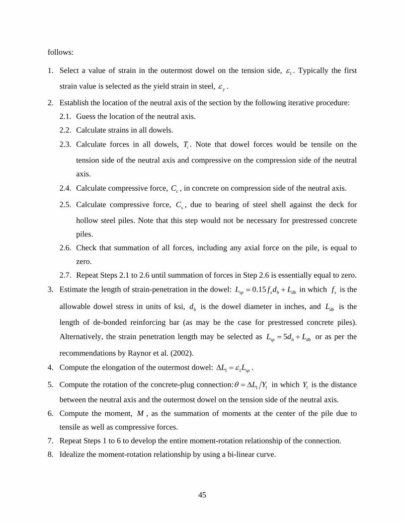
Transcript
SIMPLIFIED PROCEDURES FOR SEISMIC ANALYSIS AND
DESIGN OF PIERS AND WHARVES IN MARINE OIL AND LNG TERMINALS
by
Rakesh K. Goel California Polytechnic State University, San Luis Obispo
Research Conducted for the California State Lands Commission
Contract No. C2005-051 and
Department of the Navy, Office of Naval Research Award No. N00014-08-1-1209
Department of Civil and Environmental Engineering California Polytechnic State University, San Luis Obispo, CA 93407
June 2010
Report No. CP/SEAM-08/01
Report Documentation Page Form ApprovedOMB No. 0704-0188
Public reporting burden for the collection of information is estimated to average 1 hour per response, including the time for reviewing instructions, searching existing data sources, gathering andmaintaining the data needed, and completing and reviewing the collection of information. Send comments regarding this burden estimate or any other aspect of this collection of information,including suggestions for reducing this burden, to Washington Headquarters Services, Directorate for Information Operations and Reports, 1215 Jefferson Davis Highway, Suite 1204, ArlingtonVA 22202-4302. Respondents should be aware that notwithstanding any other provision of law, no person shall be subject to a penalty for failing to comply with a collection of information if itdoes not display a currently valid OMB control number.
1. REPORT DATE JUN 2010 2. REPORT TYPE
3. DATES COVERED 00-00-2010 to 00-00-2010
4. TITLE AND SUBTITLE Simplified Procedures for Sesmic Analysis and Design of Piers andWharves in Marine Oil and LNG Terminals
5a. CONTRACT NUMBER
5b. GRANT NUMBER
5c. PROGRAM ELEMENT NUMBER
6. AUTHOR(S) 5d. PROJECT NUMBER
5e. TASK NUMBER
5f. WORK UNIT NUMBER
7. PERFORMING ORGANIZATION NAME(S) AND ADDRESS(ES) California Polytechnic State University,Department of Civil andEnvironmental Engineering,San Luis Obispo,CA,93407
8. PERFORMING ORGANIZATIONREPORT NUMBER
9. SPONSORING/MONITORING AGENCY NAME(S) AND ADDRESS(ES) 10. SPONSOR/MONITOR’S ACRONYM(S)
11. SPONSOR/MONITOR’S REPORT NUMBER(S)
12. DISTRIBUTION/AVAILABILITY STATEMENT Approved for public release; distribution unlimited
13. SUPPLEMENTARY NOTES
14. ABSTRACT
15. SUBJECT TERMS
16. SECURITY CLASSIFICATION OF: 17. LIMITATION OF ABSTRACT Same as
Report (SAR)
18. NUMBEROF PAGES
92
19a. NAME OFRESPONSIBLE PERSON
a. REPORT unclassified
b. ABSTRACT unclassified
c. THIS PAGE unclassified
Standard Form 298 (Rev. 8-98) Prescribed by ANSI Std Z39-18
i
EXECUTIVE SUMMARY
This investigation developed simplified procedures for the seismic analysis and design of pile
supported wharves and piers in Marine Oil and LNG Terminals. A simplified coefficient-based
approach is proposed for estimating seismic displacement demand for regular structures. This
approach is adopted from the performance-based analysis procedure recently approved for
buildings in the ASCE/SEI 41-06 standard (ASCE, 2007). A modal pushover analysis (MPA)
approach is proposed for irregular structures. The MPA procedure accounts for the higher-mode
effects that are important in irregular structures (Chopra and Goel, 2004). The acceptability of
piles in terms of displacement ductility limitation, instead of the material strain limitation, is
proposed. For this purpose, simplified expressions for estimating displacement ductility capacity
of piles are recommended. These expressions are calibrated such that the material strain limits in
Title 24, California Code of Regulations, Chapter 31F, informally known as the Marine Oil
Terminal Engineering and Maintenance Standards (MOTEMS), would not be exceeded if the
displacement ductility demand is kept below the proposed displacement ductility capacity. These
simplified procedures can be used as an alternative to the procedures currently specified in the
MOTEMS. The simplified procedures can be used for preliminary design or as a quick check on
the results from detailed nonlinear analyses. The more sophisticated analysis methodology can
still be used for final design.
The following is a summary of the procedures to estimate displacement demands and
capacities for pile-supported wharves and piers.
DISPLACEMENT DEMAND
Regular Structures
It is proposed that the seismic displacement demand in a regular structure (MOTEMS 2007) be
estimated from
2
1 2 24d ATC C Sπ
Δ = (1)
in which AS is the spectral acceleration of the linear-elastic system at vibration period, T . The
coefficient 1C is given by
ii
1 2
1.0; 1.0s11.0 ; 0.2s< 1.0s
11.0 ; 0.2s0.04
TRC TaTR T
a
⎧⎪ >⎪ −⎪= + ≤⎨⎪
−⎪ + ≤⎪⎩
(2)
in which a is a site dependent constant equal to 130 for Site Class A and B, 90 for Site Class C,
and 60 for Site Class D, E, and F (definition of Site Class is available in ASCE/SEI 41-06
standard), and R is the ratio of the elastic and yield strength of the system and is defined as
A
y
S WRg V
= (3)
where W is the seismic weight of the system, yV is the yield force (or base shear) of the system,
and g is the acceleration due to gravity. The coefficient 2C is given by
22
1.0; 0.7s
1 11 ; 0.7s 800
TC R T
T
>⎧⎪= ⎨ −⎛ ⎞+ ≤⎪ ⎜ ⎟
⎝ ⎠⎩
(4)
Use of Equation (1) to compute the displacement demand should be restricted to systems
with maxR R≤ where maxR is given by
max 4
ted
y
Rα −
Δ= +Δ
(5)
in which dΔ is the smaller of the computed displacement demand, dΔ , from Equation (1) or the
displacement corresponding to the maximum strength in the pushover curve, yΔ is the yield
displacement of the idealized bilinear force-deformation curve, t is a constant computed from
( )1 0.15lnt T= + (6)
and eα is the effective post-elastic stiffness ratio computed from
( )2e P Pα α λ α α−Δ −Δ= + − (7)
where λ is a near-field effect factor equal to 0.8 for sites that are subjected to near-field effects
iii
and 0.2 for sites that are not subjected to near field effects. The near field effects may be
considered to exist if the 1 second spectral value, 1S , at the site for the maximum considered
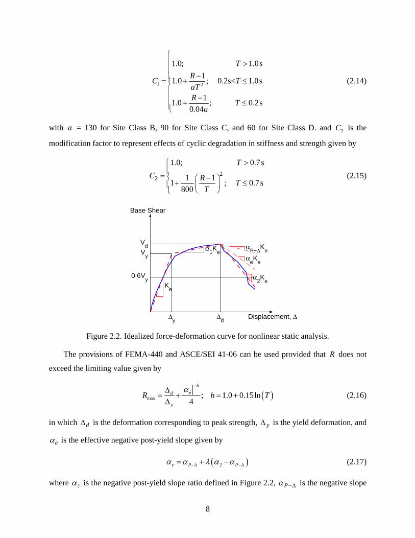
earthquake is equal to or exceeds 0.6g. The P-Delta stiffness ratio, Pα −Δ , and the maximum
negative post-elastic stiffness ratio, 2α , in Equation (7) are estimated from the idealized force-
deformation curve.
Irregular Structures
A modal pushover analysis (MPA) procedure is proposed to estimate displacement demands in
irregular Marine Oil and LNG Terminal structures (MOTEMS 2007). The following is a step-by-
step summary of the MPA procedure:
1. Compute the natural frequencies, nω and modes, nφ , for linearly elastic vibration of the
irregular Marine Oil and LNG Terminal structure.
2. Select a reference point where the displacement, rnu , is to be monitored in the selected
direction of analysis during the pushover analysis. Ideally, this reference point should be the
location on the structure with largest value of rnφ in the selected direction of analysis.
3. For the nth-mode, develop the pushover curve, bn rnV u− , for the nth modal force distribution,
*n n= Ms φ , where M is the mass matrix of the structure, and nφ is the nth mode shape. The
base shear bnV should be monitored in the same direction as the direction of the selected
reference point displacement rnu .
4. Convert the bn rnV u− pushover curve to the force-displacement, sn n nF L D− , relation for the
nth -“mode” inelastic SDF system by utilizing *sn n bn nF L V M= and n rn n rnD u φ= Γ in which
rnφ is the value of nφ at the reference point in the direction under consideration,
( )2* T Tn n n nM = M Mφ ι φ φ is the effective modal mass, and T T
n n n nΓ = M Mφ ι φ φ with ι equal to
the influence vector. The influence vector ι is a vector of size equal to the total number of
degrees of freedom. For analysis in the x-direction, the components of ι corresponding to x-
degree-of-freedom are equal to one and remaining components equal to zero. Similarly the
iv
components of ι corresponding to y-degree-of-freedom are equal to one and remaining
components equal to zero for analysis in the y-direction.
5. Idealize the force-displacement, sn n nF L D− , curve as a bilinear curve and compute the yield
value sny nF L .
6. Compute the yield strength reduction factor, ( )A sny nR S F L= .
7. Compute the peak deformation n dD = Δ of the nth-“mode” inelastic SDF system defined by
the force-deformation relation developed in Step 4 and damping ratio nζ , from Equation (1).
The elastic vibration period of the system is based on the effective slope of the sn n nF L D−
curve, which for a bilinear curve is given by ( )1/ 22n n ny snyT L D Fπ= .
8. Calculate peak reference point displacement rnu associated with the nth-“mode” inelastic
SDF system from rn n rn nu Dφ= Γ .
9. Push the structure to the reference point displacement equal to rnu and note the values of
desired displacement noδ .
10. Repeat Steps 3 to 9 for all significant modes identified.
11. Combine the peak modal displacement, noδ , by an appropriate modal combination rule, e.g.,
CQC, to obtain the peak dynamic response, oΔ .
DISPLACEMENT CAPACITY
It is proposed that the displacement capacity of piles in Marine Oil and LNG Terminals be
estimated from
c yμΔΔ = Δ (8)
where yΔ is the yield displacement of the pile and μΔ is the displacement ductility capacity of
the pile. Following are the recommendations that have been developed for the yield displacement
and displacement ductility of piles commonly used in Marine Oil and LNG Terminals. These
recommendations have been developed to ensure that the material strains in the pile at its
v
displacement capacity remain within the limits specified in the MOTEMS (2007).
The procedure to estimate the displacement capacity is intended to be a simplified procedure
for either initial design of piles or for checking results from more complex nonlinear finite
element analysis. The recommendations presented in this report are limited to: (1) piles with long
freestanding heights (length/diameter > 20) above the mud line; (2) piles with transverse
volumetric ratio greater than 0.5%; and (3) piles in which the displacement demand has been
estimated utilizing equivalent-fixity approximation. Results form this investigation should be
used with caution for parameters or cases outside of those described above.
Piles with Full-Moment- or Pin-Connection to the Deck Slab
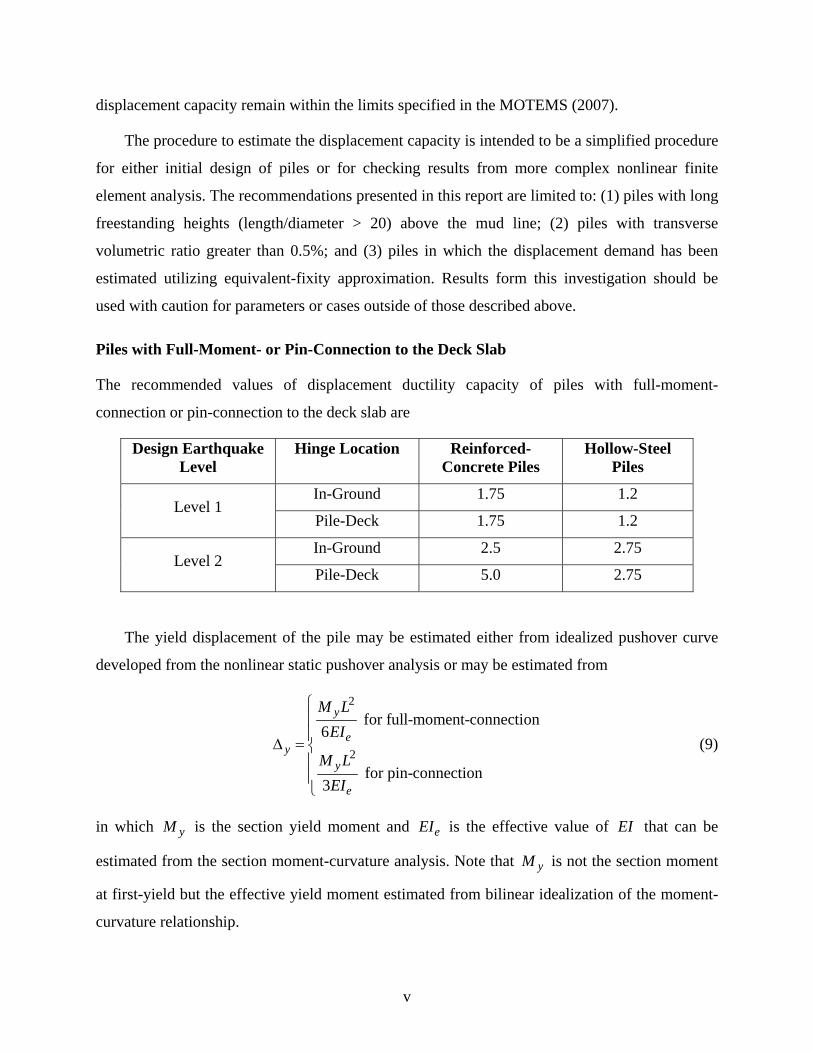
The recommended values of displacement ductility capacity of piles with full-moment-
connection or pin-connection to the deck slab are
Design Earthquake Level
Hinge Location Reinforced-Concrete Piles
Hollow-Steel Piles
In-Ground 1.75 1.2 Level 1
Pile-Deck 1.75 1.2
In-Ground 2.5 2.75 Level 2
Pile-Deck 5.0 2.75
The yield displacement of the pile may be estimated either from idealized pushover curve
developed from the nonlinear static pushover analysis or may be estimated from
2
2
for full-moment-connection6
for pin-connection 3
y
ey
y
e
M LEI
M LEI
⎧⎪⎪Δ = ⎨⎪⎪⎩
(9)
in which yM is the section yield moment and eEI is the effective value of EI that can be
estimated from the section moment-curvature analysis. Note that yM is not the section moment
at first-yield but the effective yield moment estimated from bilinear idealization of the moment-
curvature relationship.
vi
Piles with Dowel-Connection to the Deck Slab
Simplified formulas are proposed for estimating displacement ductility capacity of piles with
dowel-connection, such as hollow-steel piles or prestressed concrete piles connected to the deck
slab with dowels. The following is a step-by-step summary of the procedure to implement these
formulas to estimate displacement capacity of such piles:
1. Establish the axial load, P , on the pile.
2. Estimate the pile length based on equivalent-fixity assumption.
3. Select an appropriate design level – Level 1 or Level 2 – and establish various strain limits
for the selected design level.
4. Develop the moment-rotation relationship of the dowel-connection using the procedure
described in Chapter 8 of this report.
5. Determine rotational stiffness, kθ , yield moment, ,CyM , and yield rotation, ,Cyθ of the
dowel-connection from the moment-rotation relationship developed in Step 4.
6. Establish the rotation of the dowel-connection, Lθ , and corresponding ductility,
,CL yθμ θ θ= , when strain in the outer-most dowel of the connection reaches the strain limit
established in Step 3 for the selected design level.
7. Conduct the moment-curvature analysis of the pile section with appropriate axial load and
idealize the moment-curvature relationship by a bi-linear curve.
8. Compute the effective, eEI , and effective yield moment, y,PM , from the pile moment-
curvature relationship. Note that eEI is equal to initial elastic slope and y,PM is the yield
value of the moment of the idealized bi-linear moment-curvature relationship. For steel piles,
eEI may be computed from section properties and material modulus, and y,PM may be
17. Establish the displacement ductility capacity as lower of the values computed in Steps 15 and
16.
18. Compute the displacement capacity of the pile as product of the yield displacement computed
in Step14 and the displacement ductility capacity computed in Step 17.
The recommended value of displacement ductility for piles with full-moment-connection or
the simplified formulas for piles with dowel-connection have been shown to provide results that
are “accurate” enough for most practical applications. However, it may be useful to verify these
recommendations from experimental studies.
viii
ACKNOWLEDGMENTS
This research investigation is supported by the California State Lands Commission (CSLC)
under Contract No. C2005-051 for Development of LNGTEMS/MOTEMS Performance-Based
Seismic Criteria. This support is gratefully acknowledged. The author would especially like to
thank Martin Eskijian, CSLC Project Manager and Hosny Hakim of the CSLC for their
continuing support. The author would also like to acknowledge advice from following
individuals: Gayle Johnson and Bill Bruin of Halcrow; Bob Harn of Berger/ABAM Engineers
Inc.; Dr. Omar Jeradat of Moffatt & Nichol; Peter Yin of Port of Los Angeles; Eduardo Miranda
of Stanford University; and Dr. Hassan Sedarat and Tom Ballard of SC Solutions Inc. Finally,
the author would like to acknowledge the editorial support provided by John Freckman of the
CSLC. Additional support for this research is provided by a grant entitled "C3RP Building
Relationships 2008/2010” from the Department of the Navy, Office of Naval Research under
award No. N00014-08-1-1209. This support is also acknowledged.
ix
CONTENTS
EXECUTIVE SUMMARY ............................................................................................................. i DISPLACEMENT DEMAND..................................................................................................... i
Regular Structures.................................................................................................................... i Irregular Structures ................................................................................................................ iii
DISPLACEMENT CAPACITY ................................................................................................ iv Piles with Full-Moment- or Pin-Connection to the Deck Slab ............................................... v Piles with Dowel-Connection to the Deck Slab..................................................................... vi
ACKNOWLEDGMENTS ........................................................................................................... viii
CONTENTS................................................................................................................................... ix
2.1.1 Current MOTEMS Procedure ................................................................................. 4 2.1.2 Procedures to Compute Response of Single-Degree-of-Freedom (SDF) Systems ........ 5
8.2 MOMENT-ROTATION RELATIONSHIP OF DOWEL-CONNECTION ...................... 44
9. SIMPLIFIED MODEL OF PILE WITH DOWEL-CONNECTION........................................ 49 9.1 IDEALIZED CONNECTION AND PILE BEHAVIOR.................................................... 49
9.1.1 Moment-Rotation Behavior of Connection ................................................................. 49 9.1.2 Moment-Curvature Behavior of Pile Section .............................................................. 50 9.1.3 Force-Deformation Relationship of Pile with Dowel-Connection .............................. 51
9.2 FORCE-DEFORMATION RESPONSE OF PILE WITH DOWEL-CONNECTION ...... 52 9.2.1 Response at First Yielding in Connection ................................................................... 52 9.2.2 Response at First Yielding in Pile................................................................................ 54
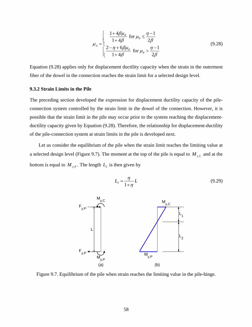
9.3 DISPLACEMENT DUCTILITY CAPACITY OF PILE ................................................... 55 9.3.1 Strain Limits in the Connection ................................................................................... 56 9.3.2 Strain Limits in the Pile ............................................................................................... 58
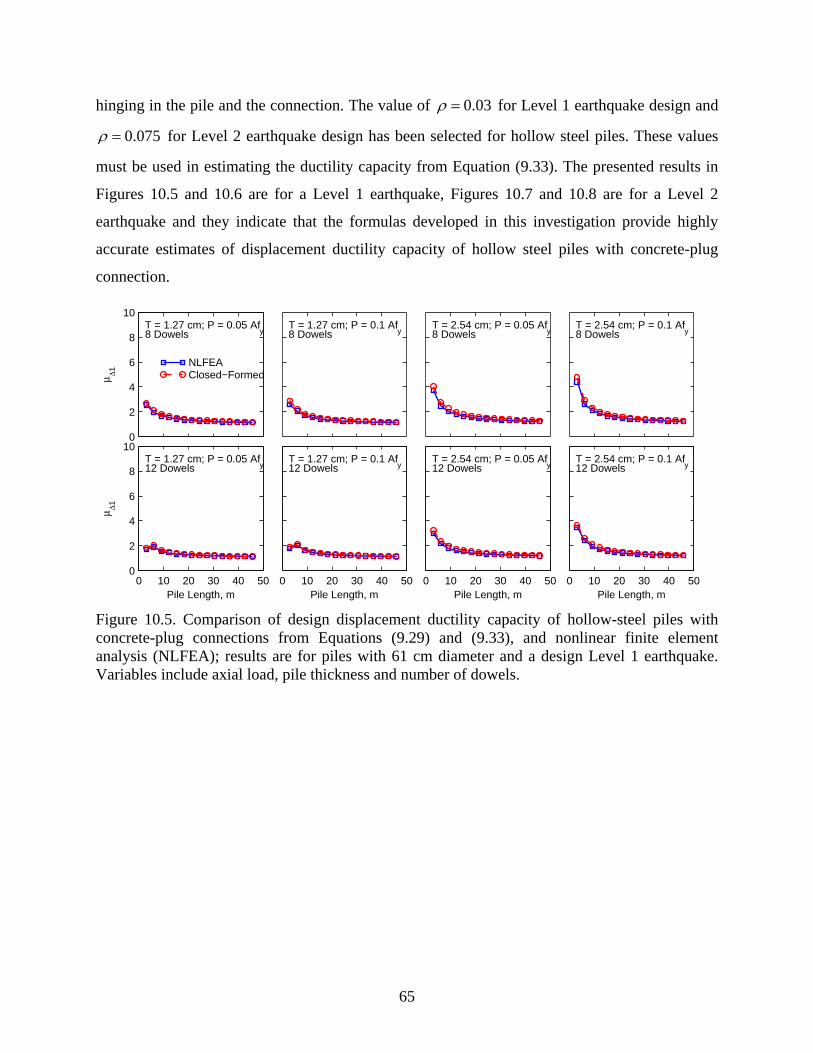
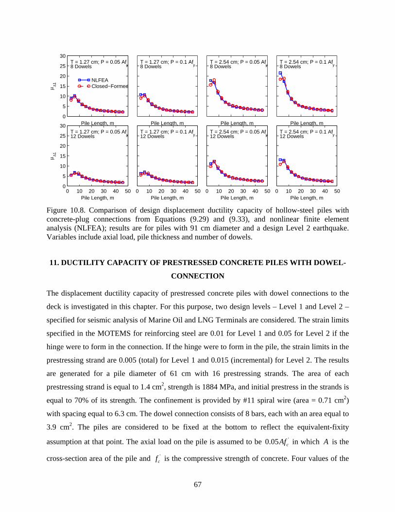
10. DUCTILITY CAPACITY OF HOLLOW STEEL PILES WITH DOWEL-CONNECTION62
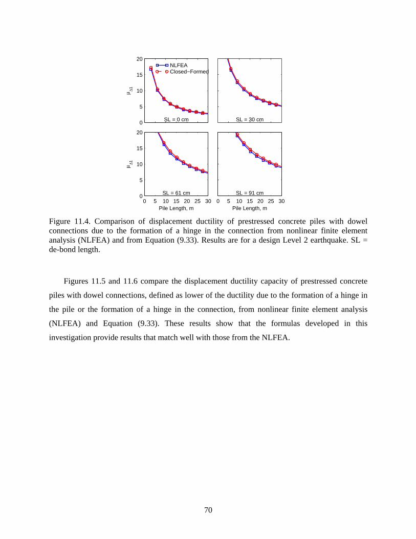
11. DUCTILITY CAPACITY OF PRESTRESSED CONCRETE PILES WITH DOWEL-CONNECTION............................................................................................................................. 67
12.2 DISPLACEMENT CAPACITY ....................................................................................... 75 12.2.1 Piles with Full-Moment- or Pin-Connection to the Deck Slab .................................. 75 12.2.2 Piles with Dowel-Connection to the Deck Slab......................................................... 76
12.3 RECOMMENDATIONS FOR FUTURE WORK ........................................................... 78
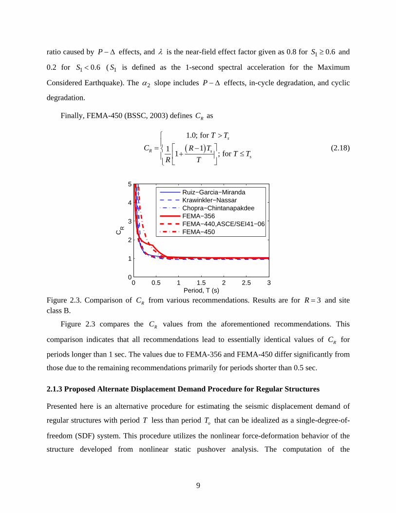
Figure 2.3. Comparison of RC from various recommendations. Results are for 3R = and site class B.
Figure 2.3 compares the RC values from the aforementioned recommendations. This
comparison indicates that all recommendations lead to essentially identical values of RC for
periods longer than 1 sec. The values due to FEMA-356 and FEMA-450 differ significantly from
those due to the remaining recommendations primarily for periods shorter than 0.5 sec.
2.1.3 Proposed Alternate Displacement Demand Procedure for Regular Structures
Presented here is an alternative procedure for estimating the seismic displacement demand of
regular structures with period T less than period oT that can be idealized as a single-degree-of-
freedom (SDF) system. This procedure utilizes the nonlinear force-deformation behavior of the
structure developed from nonlinear static pushover analysis. The computation of the
10
displacement demand is adopted from the procedure recommended in the FEMA-440 document
(ATC, 2005) and ASCE/SEI 41-06 standard (ASCE 2007). Although this procedure has been
described previously in Section 2.1.2, it is re-organized here to be compatible with the current
MOTEMS procedure. The proposed alternative procedure involves estimating the displacement
demand in a nonlinear SDF system from
2
1 2 24d ATC C Sπ
Δ = (2.19)
in which 1C and 2C are the coefficients that convert displacement demand of a linear-elastic
SDF system to displacement demand of nonlinear SDF system.
The coefficient 1C is given by
1 2
1.0; 1.0s11.0 ; 0.2s< 1.0s
11.0 ; 0.2s0.04
TRC TaTR T
a
⎧⎪ >⎪ −⎪= + ≤⎨⎪
−⎪ + ≤⎪⎩
(2.20)
in which a is a site dependent constant equal to 130 for Site Class A and B, 90 for Site Class C,
and 60 for Site Class D, E, and F; and R is the ratio of the elastic to the yield strength of the
system and is defined as
A
y
S WRg V
= (2.21)
in which AS is the spectral acceleration used in Equation (2.1), W is the seismic weight of the
system, yV is the yield force (or base shear) of the system, and g is the acceleration due to
gravity. The coefficient 2C is given by
22
1.0; 0.7s
1 11 ; 0.7s 800
TC R T
T
>⎧⎪= ⎨ −⎛ ⎞+ ≤⎪ ⎜ ⎟
⎝ ⎠⎩
(2.22)
Equation (2.19) can be used to compute the displacement demand for systems in which
maxR R≤ where maxR is given by
11
max 4
ted
y
Rα −
Δ= +Δ
(2.23)
in which dΔ is smaller than the computed displacement demand, dΔ , from Equation (2.19) or
the displacement corresponding to the maximum strength in the pushover curve, yΔ is the yield
displacement of the idealized bilinear force-deformation curve, t is a constant computed from
( )1 0.15lnt T= + (2.24)
and eα is the effective post-elastic stiffness ratio computed from
( )2e P Pα α λ α α−Δ −Δ= + − (2.25)
where λ is a near-field effect factor equal to 0.8 for sites that are subjected to near-field effects
and 0.2 for sites that are not subjected to near field effects. The near field effects may be
considered to exist if the 1 second spectral value, 1S , at the site for the maximum considered
earthquake is equal to or exceeds 0.6g. The P-Delta stiffness ratio, Pα −Δ , and the maximum
negative post-elastic stiffness ratio, 2α , in Equation (2.25) are estimated from the idealized
force-deformation curve in Figure 2.2. The Pα −Δ needed in Equation (2.25) may be estimated by
conducting pushover analysis with and without P-Delta effects.
2.2 IRREGULAR STRUCTURES
2.2.1 Current MOTEMS Procedure
The current MOTEMS procedure requires that the seismic displacement demand in irregular
concrete or steel structures with high or moderate seismic risk classification be computed from
linear modal analysis. This procedure assumes that the displacement demand in irregular
structures deformed beyond the linear elastic range may be approximated by that of a linear
elastic structure. For irregular concrete and steel structures with low seismic risk, the
displacement demand must be computed by a nonlinear static procedure; the nonlinear static
procedure for such irregular structures appears to be similar to that for regular structures.
12
2.2.2 Proposed Nonlinear Static Procedure for Irregular Structures
Presented here is a rational nonlinear static procedure for estimating displacement demand in
irregular structures. Proposed initially by Chopra and Goel (2004) to estimate seismic demands
in unsymmetric-plan buildings, this procedure has been slightly modified to estimate
displacement demands in irregular Marine Oil and LNG Terminals. The following is a step-by-
step summary of this procedure.
1. Compute the natural frequencies, nω and modes, nφ , for linearly elastic vibration of the
irregular Marine Oil and LNG Terminal.
2. Select a reference point where the displacement, rnu , is to be monitored in the selected
direction of analysis during the pushover analysis. Ideally, this reference point should be the
location on the structure with largest value of rnφ in the selected direction of analysis.
3. For the nth-mode, develop the pushover curve, bn rnV u− , for the nth modal force distribution,
*n n= Ms φ , where *
ns is the vector of lateral forces used during the pushover analysis, M is
the mass matrix of the structure, and nφ is the nth mode shape. The base shear bnV should be
monitored in the same direction as the direction of selected reference point displacement rnu .
4. Convert the bn rnV u− pushover curve to the force-displacement, sn n nF L D− , relation for the
nth -“mode” inelastic SDF system by utilizing *sn n bn nF L V M= and n rn n rnD u φ= Γ in which
rnφ is the value of nφ at the reference point in the direction under consideration,
( )2* T Tn n n nM = M Mφ ι φ φ is the effective modal mass, and T T
n n n nΓ = M Mφ ι φ φ with ι equal to
the influence vector. The influence vector ι is a vector of size equal to the total number of
degrees of freedom. For analysis in the x-direction, the components of ι corresponding to x-
degree-of-freedom are equal to one and the remaining components equal to zero. Similarly
the components of ι corresponding to y-degree-of-freedom are equal to one and the
remaining components equal to zero for analysis in the y-direction.
5. Idealize the force-displacement, sn n nF L D− , curve as a bilinear curve and compute the yield
value sny nF L .
13
6. Compute the yield strength reduction factor, ( )A sny nR S F L= .
7. Compute the peak deformation n dD = Δ of the nth-“mode” inelastic SDF system defined by
the force-deformation relation developed in Step 4 and damping ratio nζ , from Equation
(2.19). The elastic vibration period of the system is based on the effective slope of the
sn n nF L D− curve, which for a bilinear curve is given by ( )1/ 22n n ny snyT L D Fπ= .
8. Calculate peak reference point displacement rnu associated with the nth-“mode” inelastic
SDF system from rn n rn nu Dφ= Γ .
9. Push the structure to reference point displacement equal to rnu and note the values of desired
displacement noδ .
10. Repeat Steps 3 to 9 for all significant modes identified.
11. Combine the peak modal displacement, noδ , by an appropriate modal combination rule, e.g.,
CQC, to obtain the peak dynamic response, oΔ .
14
3. SIMPLIFYING ASSUMPTION
Figure 3.1b shows the mathematical model of a free-head pile of Figure 3.1a supported on
bedrock (or other competent soil) and surrounded by soil between the bedrock and mud line. In
this model, the pile is represented by beam-column elements and soil by Winkler reaction
springs connected to the pile between the bedrock and the mud line (Priestley et al., 1996). The
properties of the beam-column element are established based on the pile cross section whereas
properties of the reaction springs are specified based on geotechnical data (e.g., see Priestley et
al., 1996; Dowrick, 1987). Figure 3.1c shows the height-wise distribution of bending moment
under lateral load applied to the pile tip. Note that the maximum bending moment occurs slightly
below the mud line at a depth equal to mD , typically denoted as the depth-to-maximum-moment
below the mud line (Figure 3.1c). Lateral displacement at the pile tip can be calculated based on
this bending moment distribution or from a discrete element model implemented in most
commonly available computer programs for structural analysis.
Mud Line
Bedrock
P
F
(a)
Mud Line
P
F
(b)
Δ
Mud Line
(c)
Dm
Mud Line
Δ
(d)
L
Df
P
F
Figure 3.1. Simplified model of the pile-soil system for displacement capacity evaluation: (a) Pile supported on bedrock; (b) Mathematical model of the pile; (c) Height-wise variation of bending moment; and (d) Equivalent fixity model for displacement calculation.
An alternative approach to modeling soil flexibility effects of the pile with discrete soil
springs is the effective fixity approach (Priestley et al., 1996: Sec. 4.4.2; Dowrick, 1987: Sec.
6.4.5.3). In this approach (Figure 3.1d), the depth-to-fixity, fD , is defined as the depth that
produces in a fixed-base column with soil removed above the fixed base the same top-of-the-pile
lateral displacement under the lateral load, F , as that in the actual pile-soil system (Priestley et
al., 1996). Both the axial load, P , and top-of-the-pile moment, M (not shown in Figure 3.1d)
15
need to be considered. The depth-to-fixity, which depends on the pile diameter and soil
properties, is typically provided by the geotechnical engineer, estimated from charts available in
standard textbooks on the subject (e.g., Priestley, et al., 1996; Dowrick, 1987) or from
recommendations in several recent references (e.g., Chai, 2002; Chai and Hutchinson, 2002).
The equivalent fixity model is typically used for estimating displacement of piles that
remain within the linear-elastic range. For piles that are expected to be deformed beyond the
linear-elastic range, however, nonlinear analysis of the discrete soil spring model approach of
Figure 3.1b is recommended (Priestley et al., 1996: Sec. 4.4.2) because the plastic hinge forms at
the location of the maximum bending moment, i.e., at the depth-to-maximum-moment, mD , and
not at the depth-to-fixity, fD . A recent investigation has developed equations for estimating
lateral displacement of equivalent fixity model of the nonlinear soil-pile system by recognizing
that the plastic hinge forms at the depth-to-maximum-moment (Chai, 2002); expressions for
estimating displacement ductility capacity of pile-soil system are also available (Priestley et al.,
1996: Sec. 5.3.1). However, calculation of lateral displacement capacity of nonlinear soil-pile
systems using these approaches requires significant information about the soil properties.
This investigation uses a simplifying assumption that the equivalent fixity model may
directly be used to estimate lateral displacement capacity of nonlinear piles. Clearly, such an
approach indicates that the plastic hinge would form at the depth-to-fixity, fD , which differs
from the actual location at the depth-to-maximum-moment, mD . It is useful to note that fD is
typically in the range of 3 to 5 pile diameter whereas mD is in the range of 1 to 2 pile diameter
(see Priestley et al., 1996). Obviously, plastic hinge at fD in the equivalent fixity model would
provide slightly larger plastic displacement compared to the plastic displacement if the plastic
hinge was correctly located at mD ; note that plastic displacement is given by
( ) or p p a f mL D DθΔ = + where pθ is the plastic hinge rotation and aL is the free-standing height
of the pile. However, the simplifying assumption used in this investigation is appropriate because
difference between fD and mD is unlikely to significantly affect the plastic displacement for
piles with very long free-standing height used in marine oil terminals. Note that the freestanding
height of piles in marine oil terminals is typically in excess of twenty times the pile diameter.
16
It is useful to emphasize that the simplified approach proposed in this investigation is
intended to be used for preliminary design of piles or as a check on the results from the detailed
nonlinear analysis. It is expected that this approach would provide results that are sufficiently
“accurate” for this purpose.
The recommendations to estimate displacement capacity of the pile using the equivalent
fixity approach are strictly valid only if the displacement demand is also estimated by utilizing
the equivalent fixity pile model – a practice that is commonly used for analysis of large piers and
wharves with many piles. The recommendations developed in this report should be used with
caution if the displacement demand is estimated from a model consisting of piles with soil
springs.
17
4. MOTEMS PROCEDURE FOR CAPACITY EVALUATION OF PILES
The displacement capacity of piles in the MOTEMS is estimated from nonlinear static pushover
analysis. In this analysis, a force of increasing magnitude is applied statically in the transverse
direction (perpendicular to the pile) permitting the materials in the pile – steel and/or concrete –
to deform beyond their linear-elastic range. The displacement capacity is defined as the
maximum displacement that can occur at the tip of the pile without material strains exceeding the
permissible values corresponding to the desired design level.
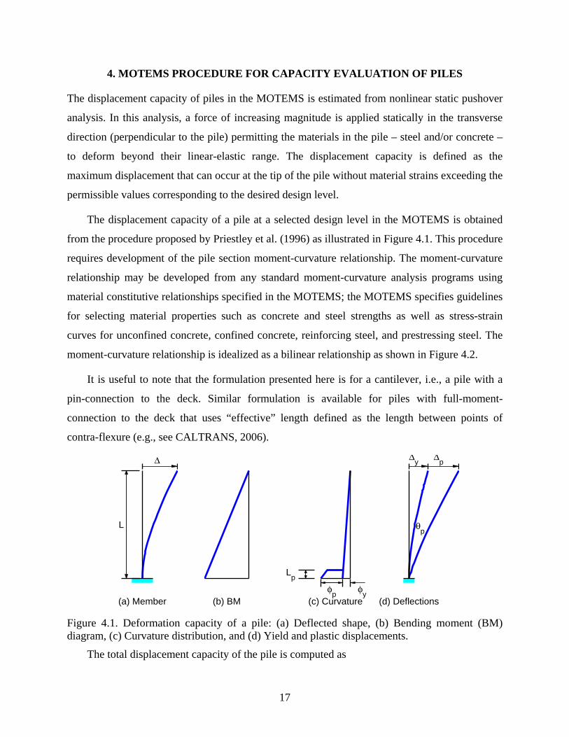
The displacement capacity of a pile at a selected design level in the MOTEMS is obtained
from the procedure proposed by Priestley et al. (1996) as illustrated in Figure 4.1. This procedure
requires development of the pile section moment-curvature relationship. The moment-curvature
relationship may be developed from any standard moment-curvature analysis programs using
material constitutive relationships specified in the MOTEMS; the MOTEMS specifies guidelines
for selecting material properties such as concrete and steel strengths as well as stress-strain
curves for unconfined concrete, confined concrete, reinforcing steel, and prestressing steel. The
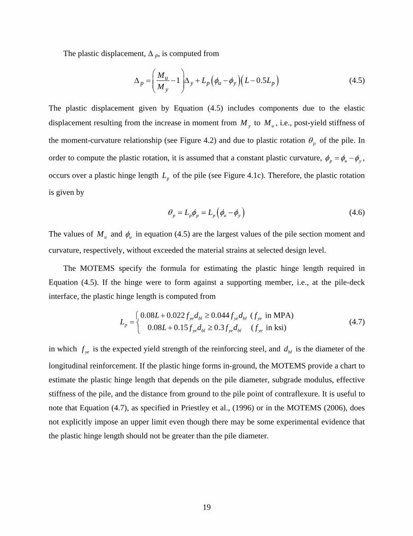
moment-curvature relationship is idealized as a bilinear relationship as shown in Figure 4.2.
It is useful to note that the formulation presented here is for a cantilever, i.e., a pile with a
pin-connection to the deck. Similar formulation is available for piles with full-moment-
connection to the deck that uses “effective” length defined as the length between points of
contra-flexure (e.g., see CALTRANS, 2006).
L
Δ
(a) Member (b) BM
Lp
φp
φy
(c) Curvature
Δy
Δp
θp
(d) Deflections
Figure 4.1. Deformation capacity of a pile: (a) Deflected shape, (b) Bending moment (BM) diagram, (c) Curvature distribution, and (d) Yield and plastic displacements.
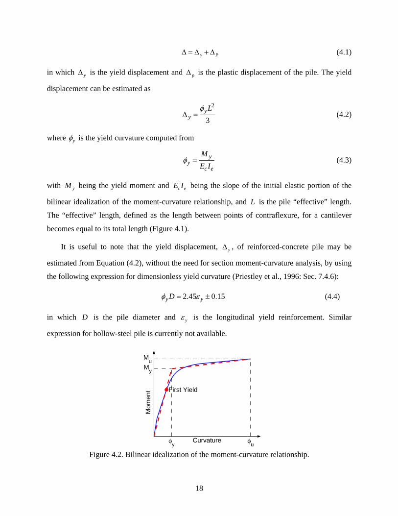
The total displacement capacity of the pile is computed as
18
y PΔ = Δ + Δ (4.1)
in which yΔ is the yield displacement and pΔ is the plastic displacement of the pile. The yield
displacement can be estimated as
2
3y
yLφ
Δ = (4.2)
where yφ is the yield curvature computed from
yy
c e
ME I
φ = (4.3)
with yM being the yield moment and c eE I being the slope of the initial elastic portion of the
bilinear idealization of the moment-curvature relationship, and L is the pile “effective” length.
The “effective” length, defined as the length between points of contraflexure, for a cantilever
becomes equal to its total length (Figure 4.1).
It is useful to note that the yield displacement, yΔ , of reinforced-concrete pile may be
estimated from Equation (4.2), without the need for section moment-curvature analysis, by using
the following expression for dimensionless yield curvature (Priestley et al., 1996: Sec. 7.4.6):
2.45 0.15y yDφ ε= ± (4.4)
in which D is the pile diameter and yε is the longitudinal yield reinforcement. Similar
expression for hollow-steel pile is currently not available.
φy
φu
My
Mu
Mom
ent
Curvature
First Yield
Figure 4.2. Bilinear idealization of the moment-curvature relationship.
19
The plastic displacement, Δ p, is computed from
( )( )1 0.5up y p u y p
y
M L L LM
φ φ⎛ ⎞
Δ = − Δ + − −⎜ ⎟⎜ ⎟⎝ ⎠
(4.5)
The plastic displacement given by Equation (4.5) includes components due to the elastic
displacement resulting from the increase in moment from yM to uM , i.e., post-yield stiffness of
the moment-curvature relationship (see Figure 4.2) and due to plastic rotation pθ of the pile. In
order to compute the plastic rotation, it is assumed that a constant plastic curvature, p u yφ φ φ= − ,
occurs over a plastic hinge length pL of the pile (see Figure 4.1c). Therefore, the plastic rotation
is given by
( )p p p p u yL Lθ φ φ φ= = − (4.6)
The values of uM and uφ in equation (4.5) are the largest values of the pile section moment and
curvature, respectively, without exceeded the material strains at selected design level.
The MOTEMS specify the formula for estimating the plastic hinge length required in
Equation (4.5). If the hinge were to form against a supporting member, i.e., at the pile-deck
interface, the plastic hinge length is computed from
0.08 0.022 0.044 ( in MPA)
0.08 0.15 0.3 ( in ksi)ye bl ye bl ye
pye bl ye bl ye
L f d f d fL
L f d f d f+ ≥⎧
= ⎨ + ≥⎩ (4.7)
in which yef is the expected yield strength of the reinforcing steel, and bld is the diameter of the
longitudinal reinforcement. If the plastic hinge forms in-ground, the MOTEMS provide a chart to
estimate the plastic hinge length that depends on the pile diameter, subgrade modulus, effective
stiffness of the pile, and the distance from ground to the pile point of contraflexure. It is useful to
note that Equation (4.7), as specified in Priestley et al., (1996) or in the MOTEMS (2006), does
not explicitly impose an upper limit even though there may be some experimental evidence that
the plastic hinge length should not be greater than the pile diameter.
20
The plastic hinge length formula of Equation (4.7) specified in the MOTEMS is based on
the recommendation by Priestley et al. (1996) for reinforced concrete sections. The MOTEMS
do not provide recommendations for plastic hinge length for steel piles or prestressed concrete
piles.
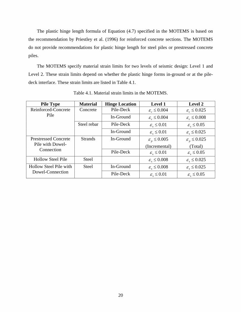
The MOTEMS specify material strain limits for two levels of seismic design: Level 1 and
Level 2. These strain limits depend on whether the plastic hinge forms in-ground or at the pile-
deck interface. These strain limits are listed in Table 4.1.
Table 4.1. Material strain limits in the MOTEMS.
Pile Type Material Hinge Location Level 1 Level 2 Pile-Deck 0.004cε ≤ 0.025cε ≤ Concrete In-Ground 0.004cε ≤ 0.008cε ≤ Pile-Deck 0.01sε ≤ 0.05sε ≤
Equation (6.5) indicates that member displacement ductility capacity can be computed directly
from the section curvature ductility capacity.
6.2 EVALUATION OF SIMPLIFIED EQUATIONS FOR DUCTILITY CAPACITY
The accuracy of Equations (6.5) in estimating displacement ductility capacity of reinforced
concrete piles at seismic design Level 2 and Level 1, respectively, is evaluated in this section.
For this purpose, displacement ductility capacity of reinforced concrete piles is evaluated from
nonlinear static pushover analysis of a finite element model. The pile is considered to be fixed at
top and bottom. These boundary conditions correspond to a pile that is connected to the pile-cap
with a full-moment connection, and utilizes the equivalent displacement fixity assumption at the
bottom. The axial load on the pile is assumed to be '0.05 g cA f in which gA is the gross cross-
25
section area of the pile and 'cf is the compressive strength of concrete. The longitudinal and
transverse reinforcements in the pile section are assumed to be equal to 1% and 0.6%,
respectively.
The pile is modeled with a nonlinear beam-column element in computer program Open
System for Earthquake Engineering Simulation (OpenSees) (McKenna and Fenves, 2001). The
distributed plasticity is considered by specifying the section properties by a fiber section model
and then using seven integration points along the element length; details of such modeling may
be found in McKenna and Fenves (2001). The material properties are specified as per the
MOTEMS specifications (MOTEMS, 2007; Mander et al., 1988).
Strains in the concrete and steel are monitored during the pushover analysis. The limiting
values of compressive strain in concrete and tensile strain in reinforcing steel are 0.004 and 0.01,
respectively, for Level 1 and 0.025 and 0.05, respectively, for Level 2. If the hinge forms below
ground, the limiting value of compressive strain in concrete and tensile strain in reinforcing steel
are 0.004 and 0.01, respectively, for Level 1 and 0.008 and 0.025, respectively, for Level 2. The
concrete strains are assumed to be specified just inside the reinforcement cage. The displacement
ductility at a selected design level corresponds to the largest displacement that can occur at the
tip of the pile without strain limits either in concrete or steel being exceeded.
The results are presented in Figure 6.1 for four pile diameters – 61 cm, 76 cm, 91 cm, and
107 cm – and pile length in the range of 5 m to 40 m. These results confirm expectations from
Equation (6.5) that the displacement ductility capacity is independent of the pile length. This
becomes apparent from essentially no variation in the ductility capacity from the nonlinear finite
element analysis of the pile lengths in Figure 6.1 for both design levels and all pile diameters.
The presented results also demonstrate that Equation (6.5) provides a very good estimate of the
displacement ductility capacity of reinforced concrete piles (see Figure 6.1).
It is useful to note that the plastic hinge length used in this investigation does not include
contribution to the plastic hinge length due to strain-penetration effects. It would be useful to
verify these findings from experiments on reinforced concrete piles.
26
1
2
3
4
5
6
7μ Δ1
, IG
or
PD
(a) Level 1, IG or PD
Pile Dia.= 61 cm
1
2
3
4
5
6
7
μ Δ2, I
G
(b) Level 2, IG
Pile Dia.= 61 cm
1
2
3
4
5
6
7
μ Δ2, P
D
(c) Level 2, PD
Pile Dia.= 61 cm
1
2
3
4
5
6
7
μ Δ1, I
G o
r P
D
Pile Dia.= 76 cm
1
2
3
4
5
6
7
μ Δ2, I
G
Pile Dia.= 76 cm
1
2
3
4
5
6
7
μ Δ2, P
D
Pile Dia.= 76 cm
1
2
3
4
5
6
7
μ Δ1, I
G o
r P
D
Pile Dia.= 91 cm
1
2
3
4
5
6
7
μ Δ2, I
G
Pile Dia.= 91 cm
1
2
3
4
5
6
7
μ Δ2, P
D
Pile Dia.= 91 cm
0 10 20 30 401
2
3
4
5
6
7
μ Δ1, I
G o
r P
D
Pile length, m
Pile Dia.= 107 cm
0 10 20 30 401
2
3
4
5
6
7
μ Δ2, I
G
Pile length, m
Pile Dia.= 107 cm
0 10 20 30 401
2
3
4
5
6
7
μ Δ2, P
D
Pile length, m
Pile Dia.= 107 cm
Figure 6.1. Displacement ductility capacity from simplified equation (shown in dashed line) and nonlinear finite element analysis (NLFEA) for seismic design (a) Level 1 for in-ground (IG) or pile-deck (PD) hinge formation, (b) Level 2 for IG hinge formation, and (c) Level 2 for PD hinge formation.
6.3 SENSITIVITY OF DISPLACEMENT DUCTILITY TO PILE PARAMETERS
6.3.1 Pile Length and Pile Diameter
Figure 6.2 presents variation of displacement ductility capacity with pile length for four values of
pile diameters: 61 cm, 76 cm, 91 cm, and 107 cm. The results are presented for piles with 1%
longitudinal reinforcement and 0.6% transverse reinforcement. As noted previously, results of
27
Figure 6.2 also indicate that the displacement ductility capacity of piles is essentially
independent of the pile length. This is expected because Equation (6.5) becomes independent of
the pile length. The results of Figure 6.2 indicate that the displacement ductility capacity of the
pile is also essentially independent of the pile diameter as apparent from almost identical curves
for the four pile diameters considered in Figure 6.2.
0 10 20 30 401
1.5
2
Pile Length, m
μ Δ1, I
G o
r P
D
(a) Level 1, IG or PD
0 10 20 30 401
2
3
4
Pile Length, m
μ Δ1, I
G
(b) Level 2, IG
0 10 20 30 401
3
5
7
Pile Length, m
μ Δ2, P
D
(c) Level 2, PD
NLFEA: Pile Dia.61 cm76 cm91 cm107 cm
Figure 6.2. Variation of displacement ductility capacity computed from nonlinear finite element analysis (NLFEA) with pile length and pile diameter: (a) Level 1 for in-ground (IG) or pile-deck (PD) hinge formation, (b) Level 2 for IG hinge formation, and (c) Level 2 for PD hinge formation.
In order to understand the aforementioned trend, i.e., independence of the displacement
ductility capacity of the pile diameter, it is useful to examine the variation of pile section
curvature ductility capacity. The results presented in Figure 6.3 indicate that the section
curvature ductility capacity is essentially independent of the pile diameter. This observation,
along with Equation (6.5), then confirms that the pile displacement ductility capacity should also
be independent of the pile diameter.
50 70 90 1100
2
4
6
Pile Diameter, cm
μ φ1, I
G o
r P
D
(a) Level 1, IG or PD
50 70 90 1100
5
10
15
20
Pile Diameter, cm
μ φ2, I
G
(b) Level 2, IG
50 70 90 1100
5
10
15
20
25
30
Pile Diameter, cm
μ φ2, P
D
(c) Level 2, PD
Figure 6.3. Variation of section curvature ductility capacity pile diameter: (a) Level 1 for in-ground (IG) or pile-deck (PD) hinge formation, (b) Level 2 for IG hinge formation, and (c) Level 2 for PD hinge formation.
28
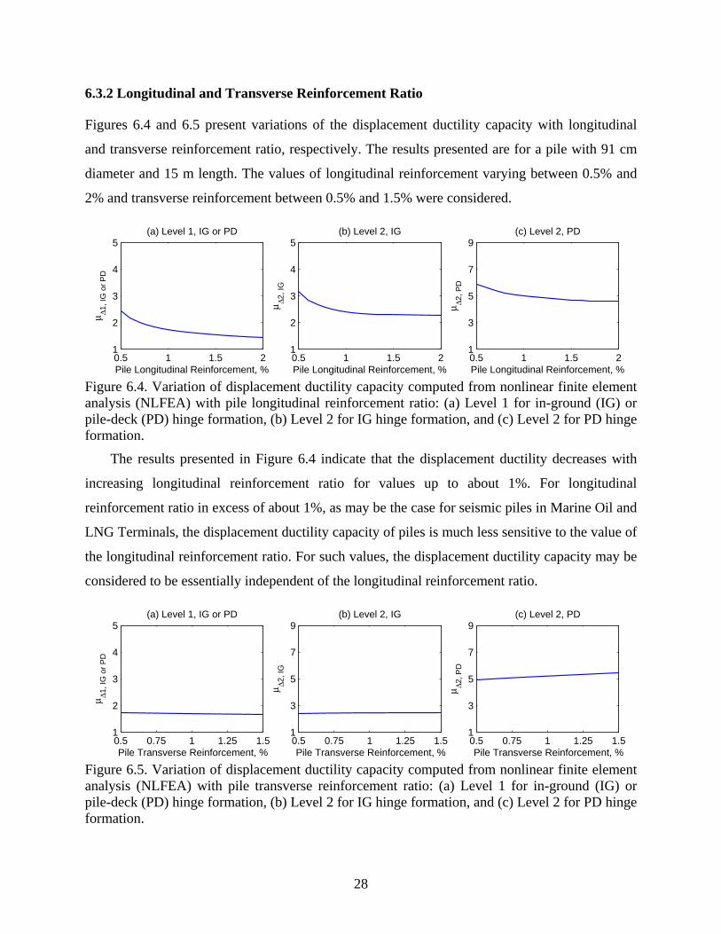
6.3.2 Longitudinal and Transverse Reinforcement Ratio
Figures 6.4 and 6.5 present variations of the displacement ductility capacity with longitudinal
and transverse reinforcement ratio, respectively. The results presented are for a pile with 91 cm
diameter and 15 m length. The values of longitudinal reinforcement varying between 0.5% and
2% and transverse reinforcement between 0.5% and 1.5% were considered.
0.5 1 1.5 21
2
3
4
5
Pile Longitudinal Reinforcement, %
μ Δ1, I
G o
r P
D
(a) Level 1, IG or PD
0.5 1 1.5 21
2
3
4
5
Pile Longitudinal Reinforcement, %
μ Δ2, I
G
(b) Level 2, IG
0.5 1 1.5 21
3
5
7
9
Pile Longitudinal Reinforcement, %
μ Δ2, P
D
(c) Level 2, PD
Figure 6.4. Variation of displacement ductility capacity computed from nonlinear finite element analysis (NLFEA) with pile longitudinal reinforcement ratio: (a) Level 1 for in-ground (IG) or pile-deck (PD) hinge formation, (b) Level 2 for IG hinge formation, and (c) Level 2 for PD hinge formation.
The results presented in Figure 6.4 indicate that the displacement ductility decreases with
increasing longitudinal reinforcement ratio for values up to about 1%. For longitudinal
reinforcement ratio in excess of about 1%, as may be the case for seismic piles in Marine Oil and
LNG Terminals, the displacement ductility capacity of piles is much less sensitive to the value of
the longitudinal reinforcement ratio. For such values, the displacement ductility capacity may be
considered to be essentially independent of the longitudinal reinforcement ratio.
0.5 0.75 1 1.25 1.51
2
3
4
5
Pile Transverse Reinforcement, %
μ Δ1, I
G o
r P
D
(a) Level 1, IG or PD
0.5 0.75 1 1.25 1.51
3
5
7
9
Pile Transverse Reinforcement, %
μ Δ2, I
G
(b) Level 2, IG
0.5 0.75 1 1.25 1.51
3
5
7
9
Pile Transverse Reinforcement, %
μ Δ2, P
D
(c) Level 2, PD
Figure 6.5. Variation of displacement ductility capacity computed from nonlinear finite element analysis (NLFEA) with pile transverse reinforcement ratio: (a) Level 1 for in-ground (IG) or pile-deck (PD) hinge formation, (b) Level 2 for IG hinge formation, and (c) Level 2 for PD hinge formation.
29
The results presented in Figure 6.5 show that displacement ductility capacity of piles does
not depend on the transverse reinforcement ratio. This becomes apparent from essentially flat
variation of the displacement ductility capacity with pile transverse reinforcement ratio.
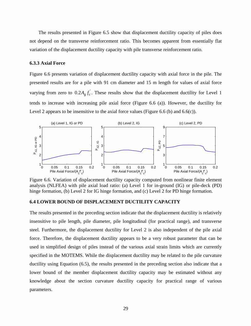
6.3.3 Axial Force
Figure 6.6 presents variation of displacement ductility capacity with axial force in the pile. The
presented results are for a pile with 91 cm diameter and 15 m length for values of axial force
varying from zero to '0.2 g cA f . These results show that the displacement ductility for Level 1
tends to increase with increasing pile axial force (Figure 6.6 (a)). However, the ductility for
Level 2 appears to be insensitive to the axial force values (Figure 6.6 (b) and 6.6(c)).
0 0.05 0.1 0.15 0.21
2
3
4
5
Pile Axial Force/(Acf′
c)
μ Δ1, I
G o
r P
D
(a) Level 1, IG or PD
0 0.05 0.1 0.15 0.21
2
3
4
5
Pile Axial Force/(Acf′
c)
μ Δ2, I
G
(b) Level 2, IG
0 0.05 0.1 0.15 0.21
3
5
7
9
Pile Axial Force/(Acf′
c)
μ Δ2, P
D
(c) Level 2, PD
Figure 6.6. Variation of displacement ductility capacity computed from nonlinear finite element analysis (NLFEA) with pile axial load ratio: (a) Level 1 for in-ground (IG) or pile-deck (PD) hinge formation, (b) Level 2 for IG hinge formation, and (c) Level 2 for PD hinge formation.
6.4 LOWER BOUND OF DISPLACEMENT DUCTILITY CAPACITY
The results presented in the preceding section indicate that the displacement ductility is relatively
insensitive to pile length, pile diameter, pile longitudinal (for practical range), and transverse
steel. Furthermore, the displacement ductility for Level 2 is also independent of the pile axial
force. Therefore, the displacement ductility appears to be a very robust parameter that can be
used in simplified design of piles instead of the various axial strain limits which are currently
specified in the MOTEMS. While the displacement ductility may be related to the pile curvature
ductility using Equation (6.5), the results presented in the preceding section also indicate that a
lower bound of the member displacement ductility capacity may be estimated without any
knowledge about the section curvature ductility capacity for practical range of various
parameters.
30
0 10 20 30 401
1.5
2
2.5
3
Pile Length, m
μ Δ1, P
D
(a) Level 1
μΔ1, PD = 1.75
0 10 20 30 401
3
5
7
Pile Length, m
μ Δ2, P
D
(b) Level 2
μΔ2, PD = 5
NLFEA: Pile Dia.61 cm76 cm91 cm107 cm
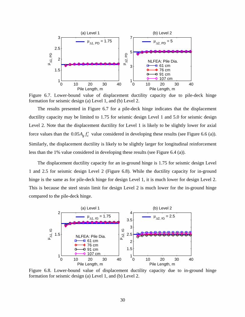
Figure 6.7. Lower-bound value of displacement ductility capacity due to pile-deck hinge formation for seismic design (a) Level 1, and (b) Level 2.
The results presented in Figure 6.7 for a pile-deck hinge indicates that the displacement
ductility capacity may be limited to 1.75 for seismic design Level 1 and 5.0 for seismic design
Level 2. Note that the displacement ductility for Level 1 is likely to be slightly lower for axial
force values than the 0.05 g cA f ′ value considered in developing these results (see Figure 6.6 (a)).
Similarly, the displacement ductility is likely to be slightly larger for longitudinal reinforcement
less than the 1% value considered in developing these results (see Figure 6.4 (a)).
The displacement ductility capacity for an in-ground hinge is 1.75 for seismic design Level
1 and 2.5 for seismic design Level 2 (Figure 6.8). While the ductility capacity for in-ground
hinge is the same as for pile-deck hinge for design Level 1, it is much lower for design Level 2.
This is because the steel strain limit for design Level 2 is much lower for the in-ground hinge
compared to the pile-deck hinge.
0 10 20 30 401
1.5
2
Pile Length, m
μ Δ1, I
G
(a) Level 1
μΔ1, IG = 1.75
NLFEA: Pile Dia.61 cm76 cm91 cm107 cm
0 10 20 30 401
1.5
2
2.5
3
3.5
4
Pile Length, m
μ Δ2, I
G
(b) Level 2
μΔ2, IG = 2.5
Figure 6.8. Lower-bound value of displacement ductility capacity due to in-ground hinge formation for seismic design (a) Level 1, and (b) Level 2.
31
6.5 SIMPLIFIED PROCEDURE TO COMPUTE DISPLACEMENT CAPACITY
Displacement capacity of piles at a selected design level may be estimated from
c yμΔΔ = Δ (6.6)
in which μΔ is the ductility capacity at a selected design level and location of hinge, i.e., equal
to 1.75 for Level 1 design and 5 for Level 2 design if the hinge were to form in the pile near the
deck, and equal to 1.75 for Level 1 and 2.5 for Level 2 if the hinge were to form in-ground, and
yΔ is the yield displacement of the pile. The yield displacement can be computed from nonlinear
pushover analysis of the pile. Alternatively, the yield displacement may be estimated based on
section yield moment and effective section eEI . For example, the yield displacement of a pile
that is fixed at the bottom and prevented from rotation at the top due to a rigid deck may be
estimated from
2
6y
ye
M LEI
Δ = (6.7)
and yield displacement of a cantilever may be estimated from
2
3y
ye
M LEI
Δ = (6.8)
in which yM is the section yield moment and eEI is the effective value of EI that can be
estimated from the section moment-curvature relationship analysis as the initial slope of the
idealized bilinear moment-curvature relationship (see Figure 4.2).
The accuracy of the procedure to estimate the displacement capacity of piles is evaluated
next. For this purpose, the approximate displacement capacity is computed first from Equation
(6.6) by utilizing the yield displacement from Equation (6.7) or (6.8) depending on the boundary
conditions. The exact displacement capacity is computed next from Equation (6.6) but with yield
displacement estimated from nonlinear static pushover analysis of the pile. For both cases, the
value of the ductility capacity obtained from the pushover analysis is used. The approximate and
exact displacement capacities are compared in Figure 6.9 for a pile with 91 cm diameter. These
32
results indicate that the approximate analysis provides an excellent estimate of the displacement
capacity of the pile for Level 1 as well as Level 2 design.
0 10 20 30 400
0.5
1
1.5
2
Pile Length, m
Δ 1, IG
or
PD
, m
(a) Level 1, IG or PD
ExactApproximate
0 10 20 30 400
0.5
1
1.5
2
2.5
3
Pile Length, mΔ 2,
IG, m
(b) Level 2, IG
0 10 20 30 400
1
2
3
4
5
Pile Length, m
Δ 2, P
D, m
(c) Level 2, PD
Figure 6.9. Comparison of displacement capacities due to pile-deck hinge formation from exact and approximate analyses.
The approximate analysis is attractive because it eliminates the need for nonlinear static
analysis of the pile. However, it must be noted that the approximate analysis may only be used
for the soil-pile-deck system that can be idealized either by a fixed-fixed column or by a
cantilever column – the two cases for which closed form solutions to estimate yield displacement
are available (see Equations 6.7 and 6.8) – using the equivalent displacement fixity concept. For
other cases, the yield displacement may have to be estimated from nonlinear static pushover
analysis of the soil-pile-deck system.
33
7. DISPLACEMENT CAPACITY OF HOLLOW STEEL PILES
This Chapter presents development of a simplified procedure for estimating displacement
capacity of hollow steel piles connected to the deck either by a pin connection or by a full-
moment-connection strong enough to force hinging in the steel pile. For this purpose, the current
approach in the MOTEMS (see Equations 4.1 to 4.6 in Chapter 4) is further simplified. Presented
first is the development of simplified equations to compute displacement ductility of hollow steel
piles that are independent of the pile length and depend only on the pile section ductility and
seismic design level. The accuracy of these equations is then evaluated against results from
nonlinear finite element analyses. Subsequently, results of a parametric study are presented to
show the sensitivity of the displacement ductility capacity on pile diameter, pile thickness, and
axial force level. Based on these results, lower bound estimates of the ductility capacity of
hollow steel piles for two design levels – Level 1 and Level 2 – are proposed. Finally, it is
demonstrated that the lower-bound displacement ductility values along with simplified
expressions for yield displacement provide very good estimates of the displacement capacity of
piles when compared against values from nonlinear finite element analysis.
7.1 THEORETICAL BACKGROUND
Similar to the displacement ductility of reinforced concrete piles, the displacement ductility
capacity of hollow steel piles may also be defined as
( )1 3 1 1 0.5p pL LL Lφμ μΔ
⎛ ⎞⎛ ⎞+ − −⎜ ⎟⎜ ⎟
⎝ ⎠⎝ ⎠ (7.1)
The MOTEMS does not explicitly provide guidelines for selecting length of the plastic hinge for
hollow steel piles. Based on calibration of results from finite element analysis against those from
Equation (7.1) (see results presented later in Figure 7.1), it was found that the following plastic
hinge lengths are appropriate for the two seismic design levels for hollow steel piles in Marine
Oil and LNG Terminals:
0.03 for Level 1pL L (7.2a)
0.075 for Level 2pL L (7.2b)
34
With the plastic hinge length selected as given by Equations (7.2(a) and 7.2(b)), Equation
(7.1) simplifies to
0.9113 0.0886 for Level 1φμ μΔ = + (7.3a)
0.7834 0.2166 for Level 2φμ μΔ = + (7.3b)
As noted previously for reinforced concrete piles, Equations (7.3(a) and 7.3(b)) for displacement
ductility capacity of hollow steel piles also indicates that the displacement ductility capacity is
independent of the pile length and it can be computed directly from the section curvature
ductility capacity. Because the plastic hinge length differs for the two design levels, the
displacement ductility also depends on the seismic design level.
7.2 EVALUATION OF SIMPLIFIED EQUATIONS FOR DUCTILITY CAPACITY
The accuracy of Equations (7.3(a) and 7.3(b)) in estimating displacement ductility capacity of
hollow steel piles at seismic design Level 1 and Level 2, respectively, is evaluated in this section.
For this purpose, displacement ductility capacity of hollow steel piles is evaluated from nonlinear
static pushover analysis of a finite element model. The pile is considered to be fixed at top and
bottom. These boundary conditions correspond to a pile that is connected to the pile-cap with a
full-moment connection that would force formation of a plastic hinge in the steel pile, and
utilizes the equivalent displacement fixity assumption at the bottom. The axial load on the pile is
assumed to be 0.05 yAf in which A is the cross section area of the pile and yf is the yield
strength of steel. The pile wall thickness is assumed to be 1.27 cm.
The pile is modeled with a nonlinear beam-column element using the computer program
“Open System for Earthquake Engineering Simulation (OpenSees)”, (McKenna and Fenves,
2001). The distributed plasticity is considered by specifying the section properties by a fiber
section model and the using seven integration points along the element length; details of such
modeling may be found in McKenna and Fenves (2001). Strains in steel are monitored during the
pushover analysis. The limiting values of strain in steel are 0.008 and 0.025 for Level 1 and
Level 2, respectively for in-ground or pile-deck hinge formation. The displacement ductility at a
selected design level corresponds to the largest displacement that can occur at the tip of the pile
without the strain limit in steel being exceeded.
35
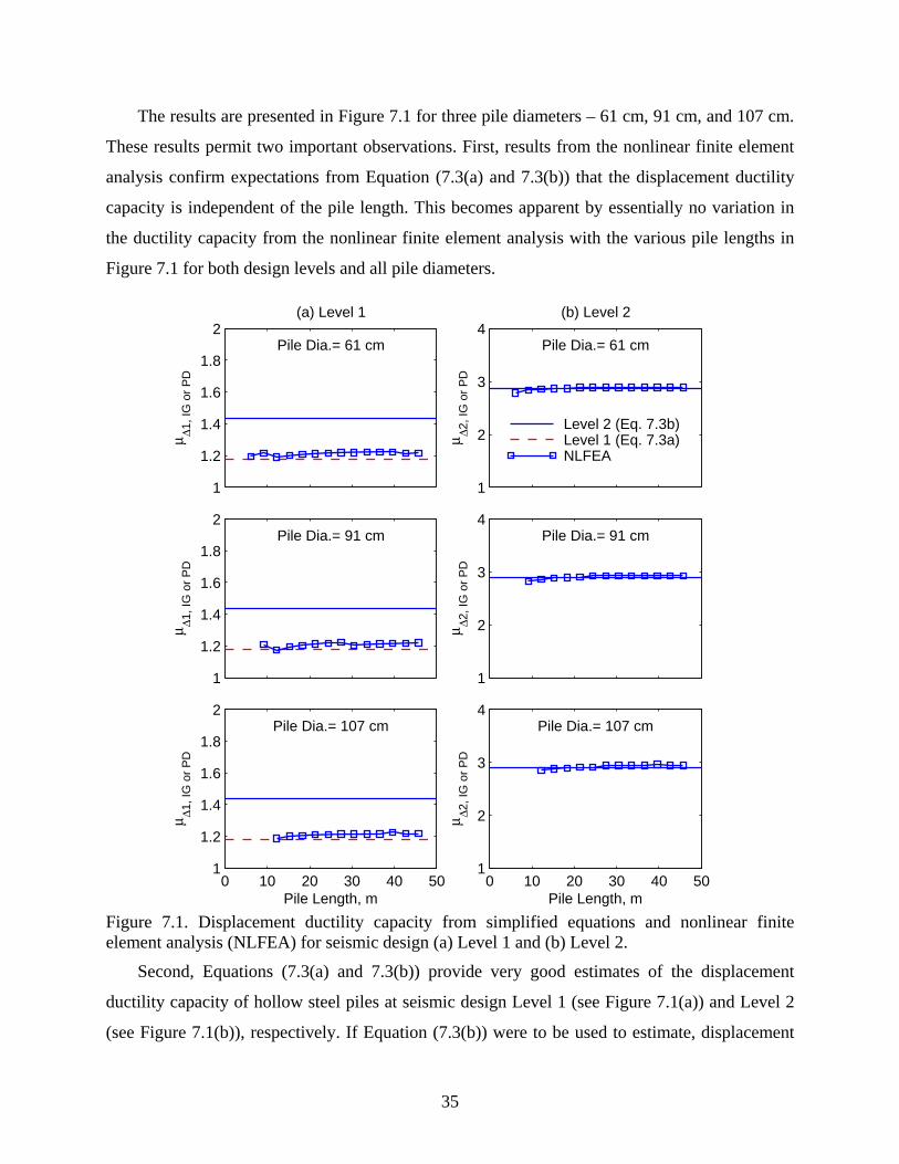
The results are presented in Figure 7.1 for three pile diameters – 61 cm, 91 cm, and 107 cm.
These results permit two important observations. First, results from the nonlinear finite element
analysis confirm expectations from Equation (7.3(a) and 7.3(b)) that the displacement ductility
capacity is independent of the pile length. This becomes apparent by essentially no variation in
the ductility capacity from the nonlinear finite element analysis with the various pile lengths in
Figure 7.1 for both design levels and all pile diameters.
1
1.2
1.4
1.6
1.8
2
μ Δ1, I
G o
r P
D
(a) Level 1
Pile Dia.= 61 cm
1
2
3
4
μ Δ2, I
G o
r P
D
(b) Level 2
Pile Dia.= 61 cm
Level 2 (Eq. 7.3b)Level 1 (Eq. 7.3a)NLFEA
1
1.2
1.4
1.6
1.8
2
μ Δ1, I
G o
r P
D
Pile Dia.= 91 cm
1
2
3
4
μ Δ2, I
G o
r P
D
Pile Dia.= 91 cm
0 10 20 30 40 501
1.2
1.4
1.6
1.8
2
μ Δ1, I
G o
r P
D
Pile Length, m
Pile Dia.= 107 cm
0 10 20 30 40 501
2
3
4
Pile Length, m
μ Δ2, I
G o
r P
D
Pile Dia.= 107 cm
Figure 7.1. Displacement ductility capacity from simplified equations and nonlinear finite element analysis (NLFEA) for seismic design (a) Level 1 and (b) Level 2.
Second, Equations (7.3(a) and 7.3(b)) provide very good estimates of the displacement
ductility capacity of hollow steel piles at seismic design Level 1 (see Figure 7.1(a)) and Level 2
(see Figure 7.1(b)), respectively. If Equation (7.3(b)) were to be used to estimate, displacement
36
ductility capacity at seismic design Level 1, it would provide an estimate that significantly
exceeds the value from nonlinear finite element analysis (see Figure 7.1(a)). Therefore, a lower
value of the plastic hinge length, as has been used in Equation (7.3(a)) for seismic design Level 1
is justified.
These results indicate that the moment-rotation relationship to be used in the concentrated
plasticity model of hollow steel piles should consider different plastic hinge lengths for the two
design levels. If the same plastic hinge length, i.e., that for seismic design Level 2, is used in the
model that computes the displacement ductility capacity for Level 1, it may significantly
overestimate the displacement capacity for that design level (Level 1).
It is useful to note that the plastic hinge length for hollow steel piles in this investigation is
proposed based on calibration against nonlinear finite element results. It would be useful to
verify these findings from experiments on hollow steel pile conducted at displacement levels that
are expected during seismic design Level 1 and Level 2.
0 10 20 30 40 501
1.2
1.4
1.6
1.8
2
Pile Length, ft
μ Δ1, I
G o
r P
D
(a) Level 1
NLFEA: Pile Dia.61 cm91 cm107 cm
0 10 20 30 40 501
2
3
4
Pile Length, ft
μ Δ2, I
G o
r P
D
(b) Level 2
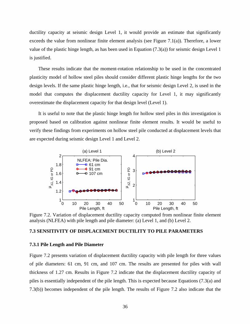
Figure 7.2. Variation of displacement ductility capacity computed from nonlinear finite element analysis (NLFEA) with pile length and pile diameter: (a) Level 1, and (b) Level 2.
7.3 SENSITIVITY OF DISPLACEMENT DUCTILITY TO PILE PARAMETERS
7.3.1 Pile Length and Pile Diameter
Figure 7.2 presents variation of displacement ductility capacity with pile length for three values
of pile diameters: 61 cm, 91 cm, and 107 cm. The results are presented for piles with wall
thickness of 1.27 cm. Results in Figure 7.2 indicate that the displacement ductility capacity of
piles is essentially independent of the pile length. This is expected because Equations (7.3(a) and
7.3(b)) becomes independent of the pile length. The results of Figure 7.2 also indicate that the
37
displacement ductility capacity of the pile is also essentially independent of the pile diameter as
apparent from almost identical curves for the three pile diameters considered.
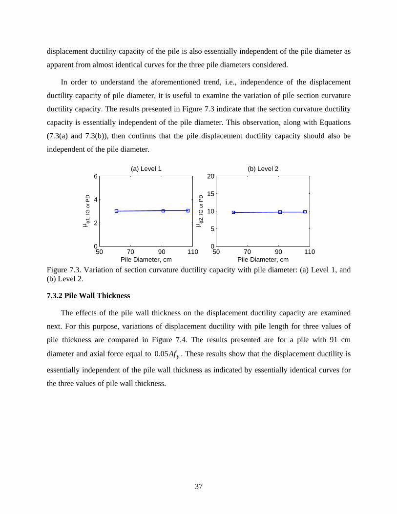
In order to understand the aforementioned trend, i.e., independence of the displacement
ductility capacity of pile diameter, it is useful to examine the variation of pile section curvature
ductility capacity. The results presented in Figure 7.3 indicate that the section curvature ductility
capacity is essentially independent of the pile diameter. This observation, along with Equations
(7.3(a) and 7.3(b)), then confirms that the pile displacement ductility capacity should also be
independent of the pile diameter.
50 70 90 1100
2
4
6
Pile Diameter, cm
μ φ1, I
G o
r P
D
(a) Level 1
50 70 90 1100
5
10
15
20
Pile Diameter, cm
μ φ2, I
G o
r P
D
(b) Level 2
Figure 7.3. Variation of section curvature ductility capacity with pile diameter: (a) Level 1, and (b) Level 2.
7.3.2 Pile Wall Thickness
The effects of the pile wall thickness on the displacement ductility capacity are examined
next. For this purpose, variations of displacement ductility with pile length for three values of
pile thickness are compared in Figure 7.4. The results presented are for a pile with 91 cm
diameter and axial force equal to 0.05 yAf . These results show that the displacement ductility is
essentially independent of the pile wall thickness as indicated by essentially identical curves for
the three values of pile wall thickness.
38
0 10 20 30 40 501
1.2
1.4
1.6
1.8
2
Pile Length, ft
μ Δ1, I
G o
r P
D
(a) Level 1
NLFEA: Wall Thickness1.27 cm2.54 cm3.81 cm
0 10 20 30 40 501
2
3
4
Pile Length, ft
μ Δ2, I
G o
r P
D
(b) Level 2
Figure 7.4. Variation of displacement ductility capacity computed from nonlinear finite element analysis (NLFEA) with pile length for three values of pile wall thickness: (a) Level 1, and (b) Level 2.
7.3.3 Axial Force
Figure 7.5 presents variation of displacement ductility capacity with axial force in the pile. The
presented results are for a pile with 91 cm diameter and 15 m length with values of axial force
varying from zero to 0.2 yAf . These results show that the displacement ductility for Level 1 is
essentially independent of the pile axial load (Figure 7.5(a)). For Level 2, while the displacement
ductility may depend on the axial load for very-low axial loads, it becomes essentially
independent of the axial load for more realistic values. However, the ductility for Level 2
appears to be insensitive to the axial force values, i.e., axial loads greater than 0.05 yAf (Figure
7.5(b)).
0 0.05 0.1 0.15 0.21
1.2
1.4
1.6
1.8
2
Pile Axial Force/(Afy)
μ Δ1, I
G o
r P
D
(a) Level 1
0 0.05 0.1 0.15 0.21
2
3
4
Pile Axial Force/(Afy)
μ Δ2, I
G o
r P
D
(b) Level 2
Figure 7.5. Variation of displacement ductility capacity computed from nonlinear finite element analysis with pile axial load ratio: (a) Level 1, and (b) Level 2.
39
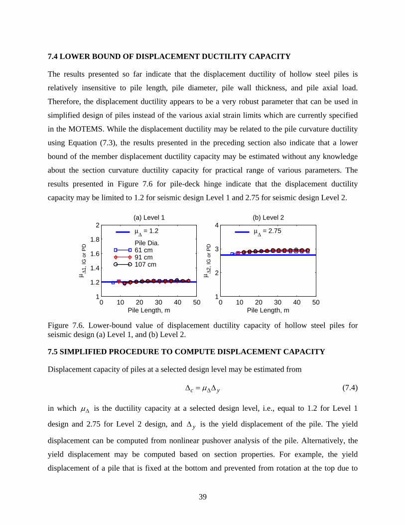
7.4 LOWER BOUND OF DISPLACEMENT DUCTILITY CAPACITY
The results presented so far indicate that the displacement ductility of hollow steel piles is
relatively insensitive to pile length, pile diameter, pile wall thickness, and pile axial load.
Therefore, the displacement ductility appears to be a very robust parameter that can be used in
simplified design of piles instead of the various axial strain limits which are currently specified
in the MOTEMS. While the displacement ductility may be related to the pile curvature ductility
using Equation (7.3), the results presented in the preceding section also indicate that a lower
bound of the member displacement ductility capacity may be estimated without any knowledge
about the section curvature ductility capacity for practical range of various parameters. The
results presented in Figure 7.6 for pile-deck hinge indicate that the displacement ductility
capacity may be limited to 1.2 for seismic design Level 1 and 2.75 for seismic design Level 2.
0 10 20 30 40 501
1.2
1.4
1.6
1.8
2
Pile Length, m
μ Δ1, I
G o
r P
D
(a) Level 1
μΔ = 1.2
Pile Dia.61 cm91 cm107 cm
0 10 20 30 40 501
2
3
4
Pile Length, m
μ Δ2, I
G o
r P
D
(b) Level 2
μΔ = 2.75
Figure 7.6. Lower-bound value of displacement ductility capacity of hollow steel piles for seismic design (a) Level 1, and (b) Level 2.
7.5 SIMPLIFIED PROCEDURE TO COMPUTE DISPLACEMENT CAPACITY
Displacement capacity of piles at a selected design level may be estimated from
c yμΔΔ = Δ (7.4)
in which μΔ is the ductility capacity at a selected design level, i.e., equal to 1.2 for Level 1
design and 2.75 for Level 2 design, and yΔ is the yield displacement of the pile. The yield
displacement can be computed from nonlinear pushover analysis of the pile. Alternatively, the
yield displacement may be computed based on section properties. For example, the yield
displacement of a pile that is fixed at the bottom and prevented from rotation at the top due to
40
rigid deck may be estimated from
2
6y
yM L
EIΔ = (7.5)
and yield displacement of a cantilever may be estimated from
2
3y
yM L
EIΔ = (7.6)
in which yM is the effective section yield moment that can be estimated from section moment-
curvature analysis and I is the section moment of inertia that can be estimated from the section
properties, and E is the modulus of elasticity for steel.
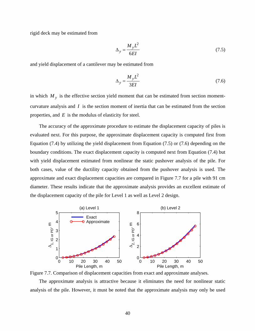
The accuracy of the approximate procedure to estimate the displacement capacity of piles is
evaluated next. For this purpose, the approximate displacement capacity is computed first from
Equation (7.4) by utilizing the yield displacement from Equation (7.5) or (7.6) depending on the
boundary conditions. The exact displacement capacity is computed next from Equation (7.4) but
with yield displacement estimated from nonlinear the static pushover analysis of the pile. For
both cases, value of the ductility capacity obtained from the pushover analysis is used. The
approximate and exact displacement capacities are compared in Figure 7.7 for a pile with 91 cm
diameter. These results indicate that the approximate analysis provides an excellent estimate of
the displacement capacity of the pile for Level 1 as well as Level 2 design.
0 10 20 30 40 500
1
2
3
4
5
Pile Length, m
Δ 1, IG
or
PD
, m
(a) Level 1
ExactApproximate
0 10 20 30 40 500
2
4
6
8
Pile Length, m
Δ 2, IG
or
PD
, m
(b) Level 2
Figure 7.7. Comparison of displacement capacities from exact and approximate analyses.
The approximate analysis is attractive because it eliminates the need for nonlinear static
analysis of the pile. However, it must be noted that the approximate analysis may only be used
41
for the soil-pile-deck system that can be idealized either by a fixed-fixed column or by a
cantilever column – the two cases for which closed form solutions to estimate yield displacement
are available (see Equations 7.5 and 7.6) – using equivalent displacement fixity concept. For
other cases, the yield displacement may have to be estimated from nonlinear static pushover
analysis of the soil-pile-deck system.
42
8. DISPLACEMENT CAPACITY OF PILES WITH DOWEL-CONNECTION
Piles are often connected to the deck using dowels. The size and number of dowel bars are
typically selected so that the moment capacity of the connection is smaller than the moment
capacity of the pile. As a result, the yielding is expected to occur in the connection rather than
the pile. The nonlinear behavior of piles with such partial-moment connection to the deck slab
may differ significantly compared to the piles with full-moment connections presented in the
previous chapters. This chapter describes two types of dowel-connections – hollow steel piles
connected to the deck by a concrete plug and dowels, and prestressed concrete piles connected to
the deck by dowels grouted into the pile and embedded in the deck concrete. Subsequently,
nonlinear behavior of such connections is examined. Finally, closed form solutions for
estimating displacement capacity of piles with partial-moment connections are presented.
8.1 DOWEL-CONNECTIONS
8.1.1 Hollow Steel Piles
Figure 8.1 shows details of the connections between a hollow steel pile and the concrete deck of
a Marine Oil or LNG Terminal. In this connection, denoted as the concrete-plug connection,
dowels are embedded in a concrete plug at the top of the pile. The concrete plug is held in place
by shear rings at its top and bottom; the shear rings would prevent the concrete plug from
slipping out (or popping-out) during lateral loads imposed by earthquakes. Others have proposed
details in which the concrete plug is held in place either by natural roughness of the inside
surface of the steel shell or use of weld-metal laid on the inside of the steel shell in a continuous
spiral in the connection region prior to placing the concrete plug (Ferritto et al., 1999). The
dowels are then embedded in the concrete deck to provide sufficient development length. A
small gap may or may not be provided between top of the pile and top of the concrete plug. This
concrete-plug connection has been shown to provide remarkable ductility capacity of hollow
steel piles (Priestley and Park, 1984; Park et al., 1987). The force transfer mechanism between
the steel pile and the concrete plug has also been investigated by Nezamian et al. (2006).
43
Steel Pipe Pile
Concrete Plug
Shear Rings
Deck
Dowel
Figure 8.1. Concrete-plug connection between hollow steel pile and concrete deck.
8.1.2 Prestressed Concrete Piles
Figure 8.2 shows details of the connections between a prestressed pile and the concrete deck of a
Marine Oil or LNG Terminal (Klusmeyer and Harn, 2004; Wray et al., 2007; Roeder et al.,
2005). Prestressed piles typically have corrugated metal sleeves that are embedded in the
concrete. These sleeves are located inside of the confined concrete core formed by the
prestressing strands and confining steel. Once the prestressed pile has been driven to the desired
depth, the dowels are grouted into the sleeves. If higher flexibility of the connection is desired, a
small portion of the dowel at the top of the pile may be wrapped in Teflon to ensure de-bonding
between the dowel and the grout. The dowels are then embedded in the concrete deck to provide
sufficient development length. Note that Figure 8.2 shows only two outermost dowels; the other
dowels are not shown to preserve clarity in the figure.
PrestressedConcrete Pile
Deck
DowelDe−BondedDowel
GroutedSleeve
Figure 8.2. Dowel-connection between prestressed concrete pile and concrete deck.
44
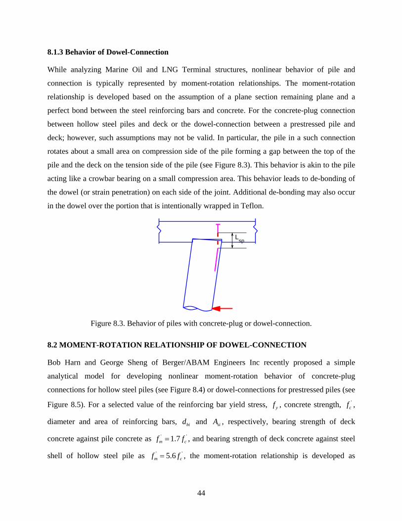
8.1.3 Behavior of Dowel-Connection
While analyzing Marine Oil and LNG Terminal structures, nonlinear behavior of pile and
connection is typically represented by moment-rotation relationships. The moment-rotation
relationship is developed based on the assumption of a plane section remaining plane and a
perfect bond between the steel reinforcing bars and concrete. For the concrete-plug connection
between hollow steel piles and deck or the dowel-connection between a prestressed pile and
deck; however, such assumptions may not be valid. In particular, the pile in a such connection
rotates about a small area on compression side of the pile forming a gap between the top of the
pile and the deck on the tension side of the pile (see Figure 8.3). This behavior is akin to the pile
acting like a crowbar bearing on a small compression area. This behavior leads to de-bonding of
the dowel (or strain penetration) on each side of the joint. Additional de-bonding may also occur
in the dowel over the portion that is intentionally wrapped in Teflon.
Lsp
Figure 8.3. Behavior of piles with concrete-plug or dowel-connection.
8.2 MOMENT-ROTATION RELATIONSHIP OF DOWEL-CONNECTION
Bob Harn and George Sheng of Berger/ABAM Engineers Inc recently proposed a simple
analytical model for developing nonlinear moment-rotation behavior of concrete-plug
connections for hollow steel piles (see Figure 8.4) or dowel-connections for prestressed piles (see
Figure 8.5). For a selected value of the reinforcing bar yield stress, yf , concrete strength, 'cf ,
diameter and area of reinforcing bars, bid and siA , respectively, bearing strength of deck
concrete against pile concrete as ' '1.7m cf f= , and bearing strength of deck concrete against steel
shell of hollow steel pile as ' '5.6m cf f= , the moment-rotation relationship is developed as
45
follows:
1. Select a value of strain in the outermost dowel on the tension side, 1ε . Typically the first
strain value is selected as the yield strain in steel, ε y .
2. Establish the location of the neutral axis of the section by the following iterative procedure:
2.1. Guess the location of the neutral axis.
2.2. Calculate strains in all dowels.
2.3. Calculate forces in all dowels, iT . Note that dowel forces would be tensile on the
tension side of the neutral axis and compressive on the compression side of the neutral
axis.
2.4. Calculate compressive force, cC , in concrete on compression side of the neutral axis.
2.5. Calculate compressive force, sC , due to bearing of steel shell against the deck for
hollow steel piles. Note that this step would not be necessary for prestressed concrete
piles.
2.6. Check that summation of all forces, including any axial force on the pile, is equal to
zero.
2.7. Repeat Steps 2.1 to 2.6 until summation of forces in Step 2.6 is essentially equal to zero.
3. Estimate the length of strain-penetration in the dowel: 0.15= +sp s b dbL f d L in which sf is the
allowable dowel stress in units of ksi, bd is the dowel diameter in inches, and dbL is the
length of de-bonded reinforcing bar (as may be the case for prestressed concrete piles).
Alternatively, the strain penetration length may be selected as 5= +sp b dbL d L or as per the
recommendations by Raynor et al. (2002).
4. Compute the elongation of the outermost dowel: 1 1 spL LεΔ = .
5. Compute the rotation of the concrete-plug connection: 1 1L Yθ = Δ in which 1Y is the distance
between the neutral axis and the outermost dowel on the tension side of the neutral axis.
6. Compute the moment, M , as the summation of moments at the center of the pile due to
tensile as well as compressive forces.
7. Repeat Steps 1 to 6 to develop the entire moment-rotation relationship of the connection.
8. Idealize the moment-rotation relationship by using a bi-linear curve.
46
5.6f′c
1.7f′c
Y1
ΔL1=ε
1L
sp
Y2
ΔLn=(Y
n/Y
1)ΔL
1
Y3Y
4Y5
θ=ΔL1/Y
1
Cs
Cc
T1T
2T3T
4
T5
P
M
Figure 8.4. Analytical model to generate the moment-rotation relationship of the concrete-plug connection between a hollow steel pile and a concrete deck.
Figures 8.6 and 8.7 show the moment rotation relationship of the concrete-plug connection
for a hollow steel pile, a dowel connection and for a prestressed concrete pile, respectively. The
nonlinear moment-rotation relationship (shown in solid line) has been idealized by a bilinear
moment-rotation relationship (shown in dashed line). It is apparent from these results that the
post-yield slope of the moment-rotation relationship is very small compared to the slope in the
linear-elastic portion. Therefore, it may be possible to simply idealize this curve with an elastic-
perfectly-plastic curve without much loss in accuracy.
47
1.7f′c
Y1
ΔL1=ε
1L
sp
Y2
ΔLn=(Y
n/Y
1)ΔL
1
Y3Y
4Y5
θ=ΔL1/Y
1
Cc
T1T
2T3T
4
T5
P
M
Figure 8.5. Analytical model to generate the moment-rotation relationship of a dowel connection between a prestressed concrete pile and a concrete deck.
48
0 0.01 0.02 0.03 0.04 0.05 0.060
200
400
600
800
Rotation, rad.
Mom
ent,
kN−
m
Figure 8.6. Moment-rotation relationship of a concrete-plug connection for hollow steel piles. The results are for a steel pile of 61 cm diameter, 1.27 cm wall thickness, axial load of 0.05 yf A , and 8 dowels each with an area of 8.2 cm2.
0 0.01 0.02 0.03 0.040
100
200
300
400
500
600
Rotation, rad.
Mom
ent,
kN−
m
Figure 8.7. Moment-rotation relationship of a dowel connection for prestressed concrete piles. The results are for a steel pile of 61 cm diameter pile, axial load of '0.05 cf A , 8 dowels each with an area of 3.9 cm2, and de-bonded length of reinforcing bars equal to 30 cm.
49
9. SIMPLIFIED MODEL OF PILE WITH DOWEL-CONNECTION
A hollow steel pile with a concrete-plug connection or a prestressed pile with a dowel connection
to the deck may be idealized as a beam-column element fixed at the base and a rotational spring
at the top (Figure 9.1). The length of the element is equal to the free-standing height of the pile
plus the depth of fixity below the mud-line. This length is selected as the length of a fixed-base
cantilever that would have same lateral displacement at the pile top as the actual pile (see
Priestley at al., 1996; Chai, 2002). The rotational spring at the top of the pile represents the
nonlinear behavior of the concrete-plug or the dowel connection. Ignoring axial deformations in
the pile, this system can be modeled with two displacement degrees-of-freedom: lateral
displacement, Δ , and rotation, θ , at the top. When a lateral force, F , is applied at the top of the
pile, a moment, M , also develops at the top due to the rotational resistance provided by the
rotational spring representing the concrete-plug or the dowel connection. Note that the rotation in
the rotational springs is equal to rotation at top of the pile.
L
Δ θ
M F
Figure 9.1. Simplified model of the pile with partial-moment connection to the deck.
Presented in this chapter is the development of a simplified procedure for estimating the
displacement capacity of hollow steel piles with concrete-plugs or prestressed piles with dowel
connections at the deck without the need to monitor strains during the pushover analysis. In
particular, formulas for estimating displacement capacity of such piles are developed.
9.1 IDEALIZED CONNECTION AND PILE BEHAVIOR
9.1.1 Moment-Rotation Behavior of Connection
The moment-rotation relationship for the concrete-plug or dowel connection between the pile
50
and the deck may be idealized as a bilinear (elastic-perfectly-plastic) curve (Figure 9.2). The
initial elastic stiffness and yield moment of the partial-moment-connection are defined by kθ and
,CyM , respectively. If Lθ is the rotation in the rotational spring when the strain in the outermost
dowel of the concrete-plug connection for hollow steel piles or the dowel connection in
prestressed concrete piles just reaches the strain limit specified for a selected design level, the
rotational ductility of the connection at specified strain limits is defined by
L
yθ
θμθ
= (9.1)
Rotation, θ
Mom
ent,
M
kθ
θy
My,Plug
θL
Figure 9.2. Idealized moment-rotation relationship of the dowel-connection.
9.1.2 Moment-Curvature Behavior of Pile Section
The moment-curvature relationship of the pile section can also be idealized as a bilinear curve
(Figure 9.3). The initial slope of this curve is equal to EI and post-yield slope is equal to EIα
in which α is the ratio of the post-yield slope and initial slope of the curve. The moment and
curvature at effective yielding of the pile are ,PyM and yφ , respectively. Note that the effective
yield moment, ,PyM , of the pile section in the idealized bi-linear moment-curvature relationship
differs slightly from the yield moment at initiation of first yielding in the outermost fiber of the
hollow steel pile or outermost strand of the prestressed concrete pile. While the ,PyM for
prestressed concrete piles should be estimated from the moment-curvature relationship, ,PyM for
51
hollow steel piles may be estimated from the formula for its plastic moment capacity as
3 3
y,P 6o i
yd dM f
⎛ ⎞−= ⎜ ⎟
⎝ ⎠ (9.2)
If Lφ is the curvature of the pile section when the material strain just reaches the strain limit
specified for a selected design level, the pile section curvature ductility is defined as
L
yφ
φμφ
= (9.3)
Curvature, φ
Mom
ent,
M
EI
φy
My,Pile
φL
ML,Pile
αEI
Figure 9.3. Idealized moment-curvature relationship of the pile section.
9.1.3 Force-Deformation Relationship of Pile with Dowel-Connection
The force-deformation behavior (or pushover curve) of a pile with fixed-base and a rotational
spring at the top may be idealized by a tri-linear relationship shown in Figure 9.3. For piles with
dowel-connections to the deck, the yield moment of the connection is typically selected to be
smaller than the yield moment of the pile section. For such a condition, the first yielding in the
pile system would occur in the connection at lateral force and displacement equal to ,CyF and
,CyΔ , respectively. Since the pile has not yet reached its yield moment, the lateral force in the
pile system would continue to increase with displacement until yielding occurs in the steel pile at
force and displacement equal to ,PyF and ,PyΔ , respectively. Subsequently, the lateral force in the
pile system would increase with displacement only due to strain-hardening effects in the pile
52
material.
Displacement, Δ
For
ce, F
Δy,C
Fy,C
Δy,P
Fy,P
Figure 9.4. Idealized pushover curve of pile with dowel-connection to the deck.
9.2 FORCE-DEFORMATION RESPONSE OF PILE WITH DOWEL-CONNECTION
This section presents development of formulas for estimating displacement capacity of piles with
dowel connections to the deck. For this purpose let us define two dimensionless constants, η and
β as
,P
,C
y
y
MM
η = (9.4)
EIk Lθ
β = (9.5)
in which η is the ratio of yield moment of the pile and the connection, and β is indicative of the
relative rotational stiffness of the pile and the connection.
9.2.1 Response at First Yielding in Connection
To compute the rotation and deflection at the top of the hollow steel pile with a concrete-plug in
the initial elastic region, i.e., ,CyΔ ≤ Δ , consider the cantilever with a moment equal to kθθ and a
lateral force equal to F at the top (Figure 9.5(a)) with a bending moment diagram (Figure
9.5(b)) and the curvature diagram (Figure 9.5(c)). Using the moment-area method for structural
53
analysis, the rotation and deflection at the top of the pile are given by
2 2
2 2k LFL FL
EI EI EIθ θ θθ
β= − = − (9.6)
and
23 3
3 2 3 2k LFL FL L
EI EI EIθθ θ
βΔ = − = − (9.7)
Equation (9.6) can be further simplified to obtain the rotation as
2
2 1FLEI
βθβ
⎛ ⎞⎛ ⎞= ⎜ ⎟⎜ ⎟+⎝ ⎠⎝ ⎠
(9.8)
Utilizing Equation (9.8), Equation (9.7) can also be simplified to obtain the deflection as
3 1 4
12 1FL
EIββ
⎛ ⎞⎛ ⎞+Δ = ⎜ ⎟⎜ ⎟+⎝ ⎠⎝ ⎠
(9.9)
The first yielding in the pushover curve (Figure 9.4) occurs at the yielding of the connection
at yield rotation at the top of the pile equal to
,C,C
yy
Mkθ
θ = (9.10)
Inserting Equation (9.10) in Equation (9.8) gives the lateral force at the yield level as
( ),C,C
21y
y
MF
Lβ= + (9.11)
and utilizing Equation (9.11) in Equation (9.9) gives the yield displacement as
( ) ( )2 2
,C ,C,C ,C
1 41 4 1 46 6
y yy y
M L k LL
EI EIθθ ββ β θ
β⎛ ⎞+
Δ = + = + = ⎜ ⎟6⎝ ⎠ (9.12)
54
L
ΔθM=kθ θF
F
FL − kθ θ(a)
FL − kθ θ
kθ θ
(b)
(FL − kθ θ)/EI
(kθ θ)/EI
(c)
Figure 9.5. Response behavior of a pile with dowel-connection up to yielding in the connection: (a) forces; (b) bending moment diagram; and (c) curvature diagram.
9.2.2 Response at First Yielding in Pile
The response in the range ,C ,Py yΔ ≤ Δ ≤ Δ may be computed by an incremental approach in
which the system may be treated as a cantilever fixed at the base and free at the top (Figure 9.6).
For this system, the incremental displacement and rotation at the top are given by
( ) ( )3
,C ,C3y yL F FEI
Δ −Δ = − (9.13)
( ) ( )2
,C ,C2y yL F FEI
θ θ− = − (9.14)
which leads to the expression for the total displacement and rotation as
( ) ( ) ( )23 3
,C,C ,C ,C1 4
3 6 3y
y y y
M LL LF F F FEI EI EI
βΔ = Δ + − = + + − (9.15)
( ) ( )2 2
,C,C ,C ,C2 2
yy y y
ML LF F F FEI k EIθ
θ θ= + − = + − (9.16)
55
L
Δ−Δy,C
θ−θy,C
F−Fy,C
F−Fy,C
(F−Fy,C
)L
(a)
(F−Fy,C
)L
(b)
(F−Fy,C
)L/EI
(c)
L
My,C
Fy,P
Fy,P
My,P
(d)
Figure 9.6. Response behavior of a pile with dowel-connection between yielding in the connection and yielding in the pile: (a) forces; (b) bending moment diagram; (c) curvature diagram; and (d) equilibrium at pile yielding.
The lateral force when the pile yields can be computed from the equilibrium of the
cantilever (Figure 9.6(d)) as
,C ,P,P L
y yy
M MF
+= (9.17)
Utilizing Equation (9.17) in Equations (9.15) and (9.16) leads to displacement and rotation at
yielding of the pile as
( ) ( )
( ) ( )
2 3,C
,P ,P ,C
2 2 2 3,C ,P ,C ,C
2,P
1 46 3
21 4 1
6 3 3 32 1
3 2
yy y y
y y y y
y
M L L F FEI EI
M L M L M L M LEI EI EI L EI
M LEI
β
β β
ηη
Δ = + + −
= + + + − +
⎛ ⎞⎛ ⎞−= ⎜ ⎟⎜ ⎟⎜ ⎟⎝ ⎠⎝ ⎠
(9.18)
( )
( )
2,C
,P ,P ,C
2,C ,P ,C ,C
,P
22
12 2 2
12
yy y y
y y y y
y
M L F Fk EI
M M L M L M Lk EI EI L EIM L
EI
θ
θ
θ
β
ηη
= + −
= + + − +
⎛ ⎞⎛ ⎞−= ⎜ ⎟⎜ ⎟
⎝ ⎠⎝ ⎠
(9.19)
9.3 DISPLACEMENT DUCTILITY CAPACITY OF PILE
This section develops the formulas for computing displacement ductility capacity of piles with a
56
partial-moment connection. Presented first are the formulas for the ductility controlled by
material strain limits in the connection. Subsequently, formulas for the ductility controlled by
material strains in the pile section are presented. The displacement ductility capacity is then
defined as the lower of the two ductility values. Finally, a step-by-step summary to compute the
displacement ductility capacity of piles with partial-moment connection is presented.
9.3.1 Strain Limits in the Connection
Let Lθ be the rotation in the connection spring for a selected design level, i.e., specified value of
strain in the outermost dowel for a selected design level. For the pile-connection system, this
rotation may occur either prior to pile yielding, i.e., ,C ,Py L yθ θ θ< < , or after pile yielding, i.e.,
,PL yθ θ> . The connection rotation ductility at onset of pile yielding is given by
,P ,P,P
,C ,C
,P
,C
12
12
12
y y
y y
y
y
M LkM EI
M k LM EI
θθ
θ
θ ημθ η
ηη
ηβ
⎛ ⎞⎛ ⎞−= = ⎜ ⎟⎜ ⎟
⎝ ⎠⎝ ⎠
⎛ ⎞ ⎛ ⎞−⎛ ⎞= ⎜ ⎟⎜ ⎟⎜ ⎟⎜ ⎟⎝ ⎠⎝ ⎠⎝ ⎠−
=
(9.20)
The displacement capacity of the pile-connection system when considering strain limits in
the outermost dowel of the connection depends on whether the pile remains elastic or the pile
yields when the dowel strain limit is reached. Note that the pile would remain elastic if θμ is less
than ,Pθμ as given by Equation (9.20). If the pile remains elastic, the rotation in the plug at a
selected design level, Lθ , is related to the lateral force F by Equation (9.16) as
17. Establish the displacement ductility capacity as the lower of the values computed in Steps 15
and 16.
18. Compute the displacement capacity of the pile as a product of the yield displacement
computed in Step14 and the displacement ductility capacity computed in Step 17.
62
10. DUCTILITY CAPACITY OF HOLLOW STEEL PILES WITH DOWEL-
CONNECTION
The displacement ductility capacity of hollow steel piles with a dowel-connection to the deck is
investigated in this chapter. For this purpose, two design levels – Level 1 and Level 2 – specified
for seismic analysis of Marine Oil and LNG Terminals in the MOTEMS are considered. The
strain limits specified in the MOTEMS for reinforcing steel are 0.01 for Level 1 and 0.05 for
Level 2 if the hinge were to form in the connection. If the hinge were to form in the steel pile
below the ground level, these strain limits are 0.008 for Level 1 and 0.025 for Level 2. Two pile
diameters – 61 cm and 91 cm – each with two wall thicknesses – 1.27 cm inch and 2.54 cm – are
considered. Furthermore, two configurations of reinforcing details in the concrete-plug
connection are considered: 8 dowels and 12 dowels, with area of each dowel being equal to 8.2
cm2. The piles are considered to be fixed at the bottom to reflect the equivalent-fixity assumption
at the bottom. The axial load on the pile is assumed to be 0.05 yAf or 0.1 yAf in which A is the
cross-section area of the pile and yf is the yield strength of steel. The pile is modeled in
computer program OPENSEES (McKenna and Fenves, 2001) using fiber section and nonlinear
beam-column elements.
Figures 10.1 to 10.4 present the variation of displacement ductility capacity of hollow-steel
piles with concrete-plug connections with pile length for two conditions: (1) formation of hinge
in the concrete-plug connection and (2) formation of hinge in the steel pile. These results were
generated by nonlinear-finite element analysis of the pile system shown in Figure 9.1. The
presented results indicate that the ductility capacity due to pile hinging tends to increase slightly
with pile length for shorter piles. For longer piles, however, the ductility capacity is essentially
independent of the pile length as apparent from the almost-flat curves. The ductility capacity due
to concrete-plug hinging, however, reduces significantly with pile length. However, this ductility
capacity may become insensitive to the pile length for longer piles.
The design ductility capacity of hollow steel piles with concrete plugs is lower for the
ductility capacities due to hinging in the steel pile and in the concrete plug. Therefore, the results
of Figures 10.1 to 10.4 also permit another important observation: hinging in the steel pile may
control the design ductility capacity of shorter piles whereas hinging in concrete-plug almost
always controls the design ductility capacity of longer piles. As such, for a given pile length, the
63
lower of the ductility capacity from hinging in the pile and hinging in the connection must be
selected as the design ductility capacity.
0
2
4
6
8
10
μ Δ1
Hinge LocationPileConnection
T = 1.27 cm; P = 0.05 Afy8 Dowels
T = 1.27 cm; P = 0.1 Afy8 Dowels
T = 2.54 cm; P = 0.05 Afy8 Dowels
T = 2.54 cm; P = 0.1 Afy8 Dowels
0 10 20 30 40 500
2
4
6
8
10
μ Δ1
Pile Length, m
T = 1.27 cm; P = 0.05 Afy12 Dowels
0 10 20 30 40 50Pile Length, m
T = 1.27 cm; P = 0.1 Afy12 Dowels
0 10 20 30 40 50Pile Length, m
T = 2.54 cm; P = 0.05 Afy12 Dowels
0 10 20 30 40 50Pile Length, m
T = 2.54 cm; P = 0.1 Afy12 Dowels
Figure 10.1. Displacement ductility capacity of hollow-steel piles with concrete-plug connections for a design Level 1 earthquake and a 61 cm pile diameter. Variables include axial load, pile thickness and number of dowels.
0
2
4
6
8
10
μ Δ1
Hinge LocationPileConnection
T = 1.27 cm; P = 0.05 Afy8 Dowels
T = 1.27 cm; P = 0.1 Afy8 Dowels
T = 2.54 cm; P = 0.05 Afy8 Dowels
T = 2.54 cm; P = 0.1 Afy8 Dowels
0 10 20 30 40 500
2
4
6
8
10
μ Δ1
Pile Length, m
T = 1.27 cm; P = 0.05 Afy12 Dowels
0 10 20 30 40 50Pile Length, m
T = 1.27 cm; P = 0.1 Afy12 Dowels
0 10 20 30 40 50Pile Length, m
T = 2.54 cm; P = 0.05 Afy12 Dowels
0 10 20 30 40 50Pile Length, m
T = 2.54 cm; P = 0.1 Afy12 Dowels
Figure 10.2. Displacement ductility capacity of hollow-steel piles with concrete-plug connections for a design Level 1 earthquake and 91 cm pile diameter. Variables include axial load, pile thickness and number of dowels.
64
0
5
10
15
20
25
30μ Δ2
T = 1.27 cm; P = 0.05 Afy8 Dowels
T = 1.27 cm; P = 0.1 Afy8 Dowels
T = 2.54 cm; P = 0.05 Afy8 Dowels
T = 2.54 cm; P = 0.1 Afy8 Dowels
0 10 20 30 40 500
5
10
15
20
25
30
μ Δ2
Pile Length, m
Hinge LocationPileConnection
T = 1.27 cm; P = 0.05 Afy12 Dowels
0 10 20 30 40 50Pile Length, m
T = 1.27 cm; P = 0.1 Afy12 Dowels
0 10 20 30 40 50Pile Length, m
T = 2.54 cm; P = 0.05 Afy12 Dowels
0 10 20 30 40 50Pile Length, m
T = 2.54 cm; P = 0.1 Afy12 Dowels
Figure 10.3. Displacement ductility capacity of hollow-steel piles with concrete-plug connections for a design Level 2 earthquake and 61 cm pile diameter. Variables include axial load, pile thickness and number of dowels.
0
5
10
15
20
25
30
μ Δ2
T = 1.27 cm; P = 0.05 Afy8 Dowels
T = 1.27 cm; P = 0.1 Afy8 Dowels
T = 2.54 cm; P = 0.05 Afy8 Dowels
T = 2.54 cm; P = 0.1 Afy8 Dowels
0 10 20 30 40 500
5
10
15
20
25
30
μ Δ2
Pile Length, m
Hinge LocationPileConnection
T = 1.27 cm; P = 0.05 Afy12 Dowels
0 10 20 30 40 50Pile Length, m
T = 1.27 cm; P = 0.1 Afy12 Dowels
0 10 20 30 40 50Pile Length, m
T = 2.54 cm; P = 0.05 Afy12 Dowels
0 10 20 30 40 50Pile Length, m
T = 2.54 cm; P = 0.1 Afy12 Dowels
Figure 10.4. Displacement ductility capacity of hollow-steel piles with concrete-plug connections for a design Level 2 earthquake and 91 cm pile diameter. Variables include axial load, pile thickness and number of dowels.
The accuracy of the formulas developed in Chapter 9 are examined next by comparing
design ductility capacity from nonlinear finite element analysis (NFEA) with that from Equations
(9.29) and (9.33). Note that the results presented are the higher of the ductility values due to
65
hinging in the pile and the connection. The value of 0.03ρ = for Level 1 earthquake design and
0.075ρ = for Level 2 earthquake design has been selected for hollow steel piles. These values
must be used in estimating the ductility capacity from Equation (9.33). The presented results in
Figures 10.5 and 10.6 are for a Level 1 earthquake, Figures 10.7 and 10.8 are for a Level 2
earthquake and they indicate that the formulas developed in this investigation provide highly
accurate estimates of displacement ductility capacity of hollow steel piles with concrete-plug
connection.
0
2
4
6
8
10
μ Δ1
NLFEAClosed−Formed
T = 1.27 cm; P = 0.05 Afy8 Dowels
T = 1.27 cm; P = 0.1 Afy8 Dowels
T = 2.54 cm; P = 0.05 Afy8 Dowels
T = 2.54 cm; P = 0.1 Afy8 Dowels
0 10 20 30 40 500
2
4
6
8
10
μ Δ1
Pile Length, m
T = 1.27 cm; P = 0.05 Afy12 Dowels
0 10 20 30 40 50Pile Length, m
T = 1.27 cm; P = 0.1 Afy12 Dowels
0 10 20 30 40 50Pile Length, m
T = 2.54 cm; P = 0.05 Afy12 Dowels
0 10 20 30 40 50Pile Length, m
T = 2.54 cm; P = 0.1 Afy12 Dowels
Figure 10.5. Comparison of design displacement ductility capacity of hollow-steel piles with concrete-plug connections from Equations (9.29) and (9.33), and nonlinear finite element analysis (NLFEA); results are for piles with 61 cm diameter and a design Level 1 earthquake. Variables include axial load, pile thickness and number of dowels.
66
0
2
4
6
8
10μ Δ1
Pile Length, m
NLFEAClosed−Formed
T = 1.27 cm; P = 0.05 Afy8 Dowels
Pile Length, m
T = 1.27 cm; P = 0.1 Afy8 Dowels
Pile Length, m
T = 2.54 cm; P = 0.05 Afy8 Dowels
Pile Length, m
T = 2.54 cm; P = 0.1 Afy8 Dowels
0 10 20 30 40 500
2
4
6
8
10
μ Δ1
Pile Length, m
T = 1.27 cm; P = 0.05 Afy12 Dowels
0 10 20 30 40 50Pile Length, m
T = 1.27 cm; P = 0.1 Afy12 Dowels
0 10 20 30 40 50Pile Length, m
T = 2.54 cm; P = 0.05 Afy12 Dowels
0 10 20 30 40 50Pile Length, m
T = 2.54 cm; P = 0.1 Afy12 Dowels
Figure 10.6. Comparison of design displacement ductility capacity of hollow-steel piles with concrete-plug connections from Equations (9.29) and (9.33), and nonlinear finite element analysis (NLFEA); results are for piles with 91 cm diameter and a design Level 1 earthquake. Variables include axial load, pile thickness and number of dowels.
0
5
10
15
20
25
30
μ Δ1
NLFEAClosed−Formed
T = 1.27 cm; P = 0.05 Afy8 Dowels
T = 1.27 cm; P = 0.1 Afy8 Dowels
T = 2.54 cm; P = 0.05 Afy8 Dowels
T = 2.54 cm; P = 0.1 Afy8 Dowels
0 10 20 30 40 500
5
10
15
20
25
30
μ Δ1
Pile Length, m
T = 1.27 cm; P = 0.05 Afy12 Dowels
0 10 20 30 40 50Pile Length, m
T = 1.27 cm; P = 0.1 Afy12 Dowels
0 10 20 30 40 50Pile Length, m
T = 2.54 cm; P = 0.05 Afy12 Dowels
0 10 20 30 40 50Pile Length, m
T = 2.54 cm; P = 0.1 Afy12 Dowels
Figure 10.7. Comparison of design displacement ductility capacity of hollow-steel piles with concrete-plug connections from Equations (9.29) and (9.33), and nonlinear finite element analysis (NLFEA); results are for piles with 61 cm diameter and a design Level 2 earthquake. Variables include axial load, pile thickness and number of dowels.
67
0
5
10
15
20
25
30μ Δ1
Pile Length, m
NLFEAClosed−Formed
T = 1.27 cm; P = 0.05 Afy8 Dowels
Pile Length, m
T = 1.27 cm; P = 0.1 Afy8 Dowels
Pile Length, m
T = 2.54 cm; P = 0.05 Afy8 Dowels
Pile Length, m
T = 2.54 cm; P = 0.1 Afy8 Dowels
0 10 20 30 40 500
5
10
15
20
25
30
μ Δ1
Pile Length, m
T = 1.27 cm; P = 0.05 Afy12 Dowels
0 10 20 30 40 50Pile Length, m
T = 1.27 cm; P = 0.1 Afy12 Dowels
0 10 20 30 40 50Pile Length, m
T = 2.54 cm; P = 0.05 Afy12 Dowels
0 10 20 30 40 50Pile Length, m
T = 2.54 cm; P = 0.1 Afy12 Dowels
Figure 10.8. Comparison of design displacement ductility capacity of hollow-steel piles with concrete-plug connections from Equations (9.29) and (9.33), and nonlinear finite element analysis (NLFEA); results are for piles with 91 cm diameter and a design Level 2 earthquake. Variables include axial load, pile thickness and number of dowels.
11. DUCTILITY CAPACITY OF PRESTRESSED CONCRETE PILES WITH DOWEL-
CONNECTION
The displacement ductility capacity of prestressed concrete piles with dowel connections to the
deck is investigated in this chapter. For this purpose, two design levels – Level 1 and Level 2 –
specified for seismic analysis of Marine Oil and LNG Terminals are considered. The strain limits
specified in the MOTEMS for reinforcing steel are 0.01 for Level 1 and 0.05 for Level 2 if the
hinge were to form in the connection. If the hinge were to form in the pile, the strain limits in the
prestressing strand are 0.005 (total) for Level 1 and 0.015 (incremental) for Level 2. The results
are generated for a pile diameter of 61 cm with 16 prestressing strands. The area of each
prestressing strand is equal to 1.4 cm2, strength is 1884 MPa, and initial prestress in the strands is
equal to 70% of its strength. The confinement is provided by #11 spiral wire (area = 0.71 cm2)
with spacing equal to 6.3 cm. The dowel connection consists of 8 bars, each with an area equal to
3.9 cm2. The piles are considered to be fixed at the bottom to reflect the equivalent-fixity
assumption at that point. The axial load on the pile is assumed to be '0.05 cAf in which A is the
cross-section area of the pile and 'cf is the compressive strength of concrete. Four values of the
68
de-bonded length of the bars in the dowel connection are considered: 0 cm, 30 cm, 61 cm, and 91
cm. The pile is modeled in computer program OPENSEES (McKenna and Fenves, 2001) using
fiber section and nonlinear beam-column elements.
Figures 11.1 and 11.2 compare the ductility of prestressed concrete piles with a dowel
connection due to the formation of a hinge in the pile from nonlinear finite element analysis
(NLFEA) and from Equation (9.33). Note that a value of 0.05ρ = has been used for both design
levels. These results show that Equation (9.33) provides results for Level 1 design that are almost
identical to those from the NLFEA (Figure 10.1). For Level 2 design, Equation (9.33) provides
results that are almost identical to those from the NLFEA for longer piles but provide a lower
bound for very short piles (Figure 11.2).
Figures 11.3 and 11.4 compare the ductility of prestressed concrete piles with a dowel
connection due to the formation of a hinge in the connection from nonlinear finite element
analysis (NLFEA) and from Equation (9.29). These results show that Equation (9.29) provides
results that are almost identical to those from the NLFEA.
0
2
4
6
8
10
μ Δ1
NLFEAClosed−Formed
SL = 0 cm SL = 30 cm
0 5 10 15 20 25 300
2
4
6
8
10
μ Δ1
Pile Length, m
SL = 61 cm
0 5 10 15 20 25 30Pile Length, m
SL = 91 cm
Figure 11.1. Comparison of displacement ductility of prestressed concrete piles with dowel connections due to the formation of a hinge in the piles from nonlinear finite element analysis (NLFEA) and from Equation (9.33). Results are for design Level 1 earthquake. SL = de-bond length.
69
0
3
6
9
12
15
μ Δ1
NLFEAClosed−Formed
SL = 0 cm SL = 30 cm
0 5 10 15 20 25 300
3
6
9
12
15μ Δ1
Pile Length, m
SL = 61 cm
0 5 10 15 20 25 30Pile Length, m
SL = 91 cm
Figure 11.2. Comparison of displacement ductility of prestressed concrete piles with dowel connections due to the formation of a hinge in the piles from nonlinear finite element analysis (NLFEA) and from Equation (9.33): results are for design Level 2 earthquake. SL = de-bond length.
0
2
4
6
8
10
μ Δ1
NLFEAClosed−Formed
SL = 0 cm SL = 30 cm
0 5 10 15 20 25 300
2
4
6
8
10
μ Δ1
Pile Length, m
SL = 61 cm
0 5 10 15 20 25 30Pile Length, m
SL = 91 cm
Figure 11.3. Comparison of displacement ductility of prestressed concrete piles with dowel connections due to the formation of a hinge in the connection from nonlinear finite element analysis (NLFEA) and from Equation (9.33). Results are for a design Level 1 earthquake. SL = de-bond length.
70
0
5
10
15
20
μ Δ1
NLFEAClosed−Formed
SL = 0 cm SL = 30 cm
0 5 10 15 20 25 300
5
10
15
20μ Δ1
Pile Length, m
SL = 61 cm
0 5 10 15 20 25 30Pile Length, m
SL = 91 cm
Figure 11.4. Comparison of displacement ductility of prestressed concrete piles with dowel connections due to the formation of a hinge in the connection from nonlinear finite element analysis (NLFEA) and from Equation (9.33). Results are for a design Level 2 earthquake. SL = de-bond length.
Figures 11.5 and 11.6 compare the displacement ductility capacity of prestressed concrete
piles with dowel connections, defined as lower of the ductility due to the formation of a hinge in
the pile or the formation of a hinge in the connection, from nonlinear finite element analysis
(NLFEA) and Equation (9.33). These results show that the formulas developed in this
investigation provide results that match well with those from the NLFEA.
71
0
2
4
6
8
10
μ Δ1
NLFEAClosed−Formed
SL = 0 cm SL = 30 cm
0 5 10 15 20 25 300
2
4
6
8
10μ Δ1
Pile Length, m
SL = 61 cm
0 5 10 15 20 25 30Pile Length, m
SL = 91 cm
Figure 11.5. Comparison of displacement ductility capacity of prestressed concrete piles with dowel connections, defined as the lower of the ductility due to the formation of a hinge in the pile or the formation of a hinge in the connection, from nonlinear finite element analysis (NLFEA) and from Equation (9.33). Results are for a design Level 1 earthquake. SL = de-bond length.
0
2
4
6
8
10
μ Δ1
SL = 0 cm SL = 30 cm
0 5 10 15 20 25 300
2
4
6
8
10
μ Δ1
Pile Length, m
SL = 61 cm
NLFEAClosed−Formed
0 5 10 15 20 25 30Pile Length, m
SL = 91 cm
Figure 11.6. Comparison of displacement ductility capacity of prestressed concrete piles with dowel connections, defined as the lower of the ductility due to the formation of a hinge in the pile or the formation of a hinge in the connection, from nonlinear finite element analysis (NLFEA) and from Equation (9.33). Results are for a design Level 2 earthquake. SL= de-bond length.
72
12. RECOMMENDATIONS
The following simplified procedures are recommended for estimating seismic displacement
demand and capacity of pile in Marine Oil and LNG Terminals. The seismic displacement
capacity recommended here is consistent with the strain limits specified in the MOTEMS.
12.1 DISPLACEMENT DEMAND
12.1.1 Regular Structures
It is recommended that the seismic displacement demand in a regular structure (MOTEMS 2007)
be estimated from the following procedure that was recently proposed in the ASCE/SEI 41-06
standard:
2
1 2 24d ATC C Sπ
Δ = (12.1)
in which AS is the spectral acceleration of the linear-elastic system at vibration period, T . The
coefficient 1C is given by
1 2
1.0; 1.0s11.0 ; 0.2s< 1.0s
11.0 ; 0.2s0.04
TRC TaTR T
a
⎧⎪ >⎪ −⎪= + ≤⎨⎪
−⎪ + ≤⎪⎩
(12.2)
in which a is a site dependent constant equal to 130 for Site Class A and B, 90 for Site Class C,
and 60 for Site Class D, E, and F (definition of Site Class is available in ASCE/SEI 41-06
standard), and R is the ratio of the elastic and yield strength of the system and is defined as
A
y
S WRg V
= (12.3)
where W is the seismic weight of the system, yV is the yield force (or base shear) of the system,
and g is the acceleration due to gravity. The coefficient 2C is given by
73
22
1.0; 0.7s
1 11 ; 0.7s 800
TC R T
T
>⎧⎪= ⎨ −⎛ ⎞+ ≤⎪ ⎜ ⎟
⎝ ⎠⎩
(12.4)
The estimation of displacement demand should be restricted to systems with
4
ted
y
Rα −
Δ≤ +Δ
(12.5)
in which dΔ is the smaller of the computed displacement demand, dΔ , or the displacement
corresponding to the maximum strength in the pushover curve, yΔ is the yield displacement of
the idealized bilinear force-deformation curve, ( )1 0.15lnt T= + , and eα is the effective post-
elastic stiffness ratio computed from
( )2e P Pα α λ α α−Δ −Δ= + − (12.6)
where λ is a near-field effect factor equal to 0.8 for sites that are subjected to near-field effects
and 0.2 for sites that are not subjected to near field effects. The near field effects may be
considered to exist if the 1 second spectral value, 1S , at the site for the maximum considered
earthquake is equal to or exceeds 0.6g. The P-Delta stiffness ratio, Pα −Δ , and the maximum
negative post-elastic stiffness ratio, 2α , are estimated from the idealized force-deformation
curve.
12.1.2 Irregular Structures
The following modal pushover analysis (MPA) procedure is recommended to estimate
displacement demands in irregular Marine Oil and LNG Terminal structures (MOTEMS 2007):
1. Compute the natural frequencies, nω and modes, nφ , for linearly elastic vibration of the
irregular Marine Oil and LNG Terminal structure.
2. Select a reference point where the displacement, rnu , is to be monitored in the selected
direction of analysis during the pushover analysis. Ideally, this reference point should be the
location on the structure with largest value of rnφ in the selected direction of analysis.
74
3. For the nth-mode, develop the pushover curve, bn rnV u− , for the nth modal force distribution,
*n n= Ms φ , where M is the mass matrix of the structure, and nφ is the nth mode shape. The
base shear bnV should be monitored in the same direction as the direction of the selected
reference point displacement rnu .
4. Convert the bn rnV u− pushover curve to the force-displacement, sn n nF L D− , relation for the
nth -“mode” inelastic SDF system by utilizing *sn n bn nF L V M= and n rn n rnD u φ= Γ in which
rnφ is the value of nφ at the reference point in the direction under consideration,
( )2* T Tn n n nM = M Mφ ι φ φ is the effective modal mass, and T T
n n n nΓ = M Mφ ι φ φ with ι equal to
the influence vector. The influence vector ι is a vector of size equal to the total number of
degrees of freedom. For analysis in the x-direction, the components of ι corresponding to x-
degree-of-freedom are equal to one and remaining components equal to zero. Similarly the
components of ι corresponding to y-degree-of-freedom are equal to one and remaining
components equal to zero for analysis in the y-direction.
5. Idealize the force-displacement, sn n nF L D− , curve as a bilinear curve and compute the yield
value sny nF L .
6. Compute the yield strength reduction factor, ( )A sny nR S F L= .
7. Compute the peak deformation n dD = Δ of the nth-“mode” inelastic SDF system defined by
the force-deformation relation developed in Step 4 and damping ratio nζ , from Equation (1).
The elastic vibration period of the system is based on the effective slope of the sn n nF L D−
curve, which for a bilinear curve is given by ( )1/ 22n n ny snyT L D Fπ= .
8. Calculate peak reference point displacement rnu associated with the nth-“mode” inelastic
SDF system from rn n rn nu Dφ= Γ .
9. Push the structure to the reference point displacement equal to rnu and note the values of
desired displacement noδ .
75
10. Repeat Steps 3 to 9 for all significant modes identified.
11. Combine the peak modal displacement, noδ , by an appropriate modal combination rule, e.g.,
CQC, to obtain the peak dynamic response, oΔ .
12.2 DISPLACEMENT CAPACITY
It is recommended that the displacement capacity of piles in Marine Oil and LNG Terminals be
estimated from
c yμΔΔ = Δ (12.7)
where yΔ is the yield displacement of the pile and μΔ is the displacement ductility capacity of
the pile.
The procedure to estimate the displacement capacity is intended to be a simplified procedure
for either initial design of piles or for checking results from more complex nonlinear finite
element analysis. The recommendations presented here are limited to: (1) piles with long
freestanding heights (length/diameter > 20) above the mud line; (2) piles with transverse
volumetric ratio greater than 0.5%; and (3) piles in which the displacement demand has been
estimated utilizing equivalent-fixity approximation. Results form this investigation should be
used with caution for parameters or cases outside of those described above.
12.2.1 Piles with Full-Moment- or Pin-Connection to the Deck Slab
The recommended values of displacement ductility capacity of piles with full-moment-
connection or pin-connection to the deck slab are
Design Earthquake Level
Hinge Location Reinforced-Concrete Piles
Hollow-Steel Piles
In-Ground 1.75 1.2 Level 1
Pile-Deck 1.75 1.2
In-Ground 2.5 2.75 Level 2
Pile-Deck 5.0 2.75
76
The yield displacement of the pile may be estimated either from idealized pushover curve
developed from the nonlinear static pushover analysis or may be estimated from
2
2
for full-moment-connection6
for pin-connection 3
y
ey
y
e
M LEI
M LEI
⎧⎪⎪Δ = ⎨⎪⎪⎩
(12.8)
in which yM is the section yield moment and eEI is the effective value of EI . Note that yM is
not the section moment at first-yield but the effective yield moment estimated from bilinear
idealization of the moment-curvature relationship.
12.2.2 Piles with Dowel-Connection to the Deck Slab
The following procedure is recommended for estimating displacement ductility capacity of piles
with dowel-connection, such as hollow-steel piles or prestressed concrete piles connected to the
deck slab with dowels:
1. Establish the axial load, P , on the pile.
2. Estimate the pile length based on equivalent-fixity assumption.
3. Select an appropriate design level – Level 1 or Level 2 – and establish various strain limits
for the selected design level.
4. Develop the moment-rotation relationship of the dowel-connection using the procedure
described in Chapter 8 of this report.
5. Determine rotational stiffness, kθ , yield moment, ,CyM , and yield rotation, ,Cyθ of the
dowel-connection from the moment-rotation relationship developed in Step 4.
6. Establish the rotation of the dowel-connection, Lθ , and corresponding ductility,
,CL yθμ θ θ= , when strain in the outer-most dowel of the connection reaches the strain limit
established in Step 3 for the selected design level.
7. Conduct the moment-curvature analysis of the pile section with appropriate axial load and
idealize the moment-curvature relationship by a bi-linear curve.
77
8. Compute the effective, eEI , and effective yield moment, y,PM , from the pile moment-
curvature relationship. Note that eEI is equal to initial elastic slope and y,PM is the yield
value of the moment of the idealized bi-linear moment-curvature relationship. For steel piles,
eEI may be computed from section properties and material modulus, and y,PM may be