Page 1
Simula'onThechallengefordatascience
Oxford Man InstituteMarch 9, 2018
J.DoyneFarmerMathema'calIns'tute,ComputerScienceDept.and
Ins'tuteforNewEconomicThinkingattheOxfordMar'nSchoolExternalprofessor,SantaFeIns'tute
Page 2
Computation has revolutionized physical and natural science
• Makes it possible to study nonlinear dynamics and complex systems.
• Over the last 50 years this has been the most important driver of progress in science.
• Social science (including economics) has not benefitted like physical and natural science.– elementary processes are not well understood– different cultural attitudes 2
Page 3
Bigdataandmachinelearning
• Computerhasalsogivenusbigdata• Machinelearning– fiGnganonlinearfunc'ontolotsofdata– difficulttomodelsitua'onsithasneverseen
• Simula'onsarebasedonanunderstandingofhowthingswork– canusebigdataforcalibra'on– candopolicyanalysis
3
Page 4
Simula'oninsocialscienceleadstoABM
• Agent-basedmodels(ABMs)areaclassofcomputa'onalmodelsforsimula'ngtheac'onsandinterac'onsofautonomousagents(individualsorcollec'veen''essuchasorganiza'onsorgroups)withaviewtoassessingtheireffectsonthesystemasawhole.
4
Page 5
Whyagent-basedmodeling?• Diversifies toolkit of economics: Complements
DSGE and econometric models.• Time is ripe: increased computer power, Big Data,
behavioral knowledge. • Hasn’t really been tried yet -- crude estimates:
– econometric models: 30,000 person-years– DSGE models: 20,000 person-years– agent-based models: 500 person-years
• Successes elsewhere: Traffic, epidemiology, defense
• Examples of successes in economics: – Endogenous explanations of clustered volatility and
heavy tails; firm size; neighborhood choice
5
Page 6
Advantages• Can faithfully represent real institutions• Easily captures instabilities, feedback,
nonlinearities, heterogeneity, network structure,...• Can capture endogenous dynamics• Easy to do policy testing• Easy to incorporate behavioral knowledge• Can calibrate modules independently using micro
data -- much stronger test of models!– In some sense between theory and econometrics
• ABMs synthesize knowledge: – Possible to understand what is not understood
6
Page 7
Designphilosophy• Assimpleaspossible• Designmodelaroundavailabledata• Fitmodulesandagentbehaviorsindependentlyfrom
targetdata,usingseveraldifferentmethods:– micro-dataforcalibra'onandtes'ng– consultdomainexpertsforbehavioralhypotheses– adap'veop'miza'ontocopewithLucascri'que– economicexperiments
• Systema'callyexploremodelsensi'vi'es• Plugandplay• Standardizedinterfaces• Industrialcode,soZwarestandards,opensource
7
Page 8
Formula'ngdecisionrules
• Makesomethingup• Takefrombehavioralliterature• PerformexperimentsincontextofABM• Interviewdomainexperts• Calibrateagainstmicrodata• Learningandselec'on,Lucascri'que• Ra'onality
8
Page 9
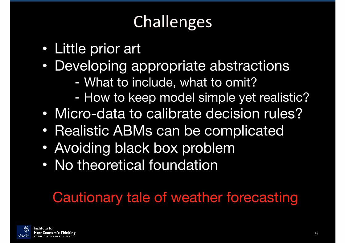
Challenges• Little prior art • Developing appropriate abstractions
- What to include, what to omit?- How to keep model simple yet realistic?
• Micro-data to calibrate decision rules?• Realistic ABMs can be complicated• Avoiding black box problem• No theoretical foundation
Cautionary tale of weather forecasting
9
Page 10
Housingmarkets
10
Page 11
Washingtonhousingmodelproject
• Seniorcollaborators:RobAxtell,JohnGeanakoplos,PeterHowie
• Juniorcollaborators:ErnestoCarella,BenConlee,JonGoldstein,MaehewHendrey,PhilipKalikman
11
Page 12
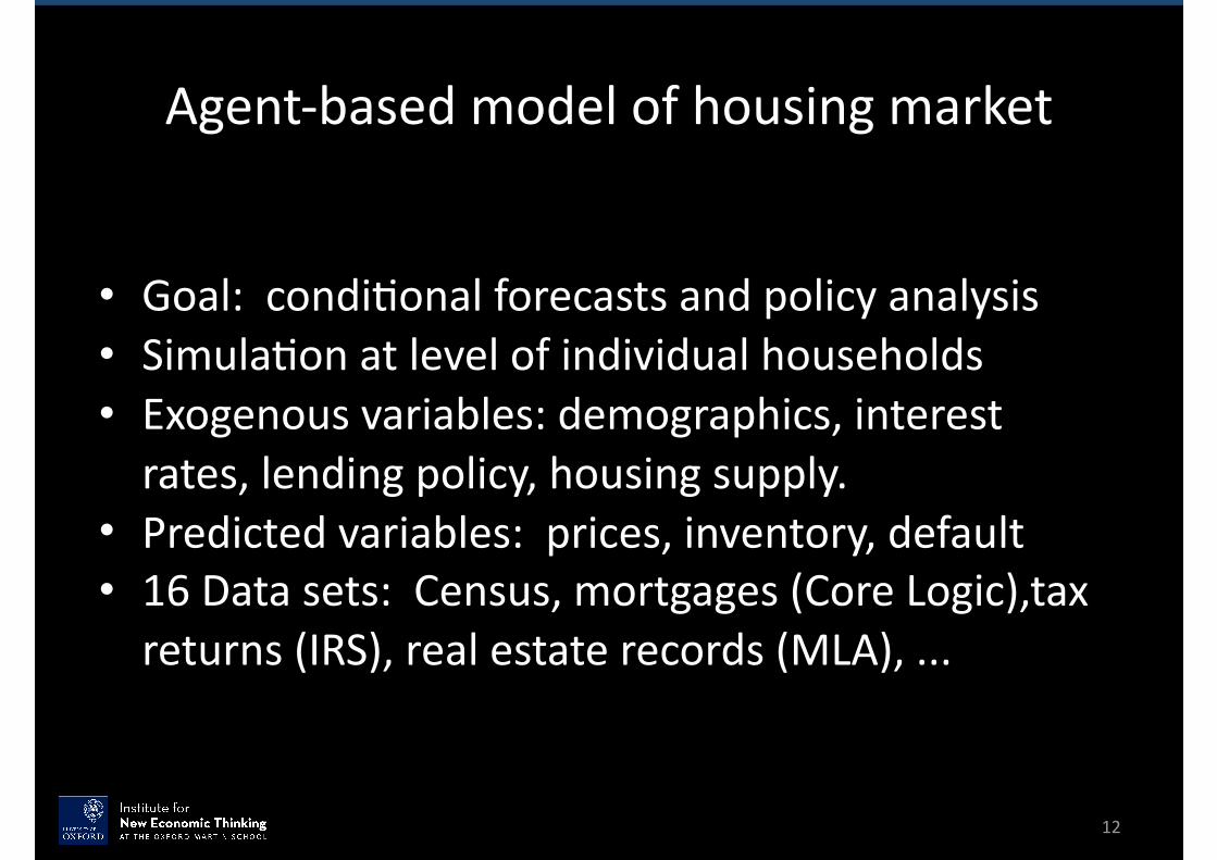
Agent-basedmodelofhousingmarket
• Goal:condi'onalforecastsandpolicyanalysis• Simula'onatlevelofindividualhouseholds• Exogenousvariables:demographics,interestrates,lendingpolicy,housingsupply.
• Predictedvariables:prices,inventory,default• 16Datasets:Census,mortgages(CoreLogic),taxreturns(IRS),realestaterecords(MLA),...
12
Page 13
Moduleexamples• Desiredexpendituremodel– buyers’desiredhomepriceasafunc'onofhouseholdincomeandwealth
• Seller’spricingmodel– seller’sofferingpriceasafunc'onofhomequality,'meonmarket,andtotalinventory
• Buyer-sellermatchingalgorithm– linksbuyersandsellerstomaketransac'ons
• Householdwealthdynamics– modelsconsump'onandsavings
• Loanapproval– qualifiesbuyersforloansbasedonincome,wealth;mustmatchissuedmortgages
13
Page 14
HousingmodelalgorithmAteach'mestep:
• Inputchangestoexogenousvariables• Updatestateofhouseholds– income,consump'on,wealth,foreclosures,...
• Buyers:–Who?Pricerange?Loanapproval,terms?
• Sellers:–Who?Offeringprice?Priceupdates?
• Matchbuyersandsellers– Computetransac'onsandprices
14
Page 15
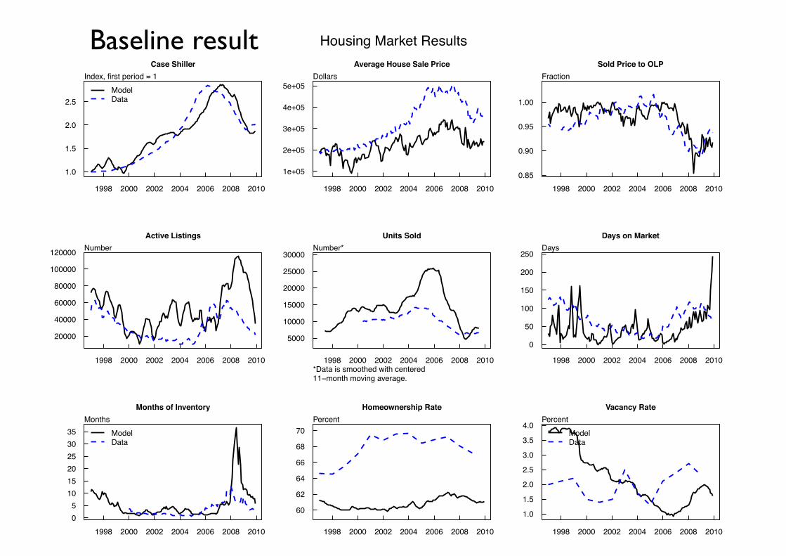
Resultswhenwefitparameterstomatchthetargetdata
15
Page 16
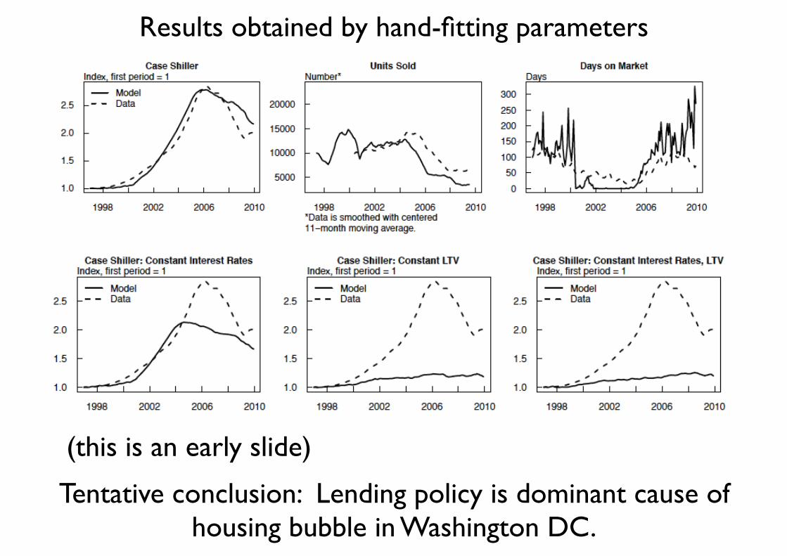
Tentative conclusion: Lending policy is dominant cause of housing bubble in Washington DC.
Results obtained by hand-fitting parameters
(this is an early slide)
Page 17
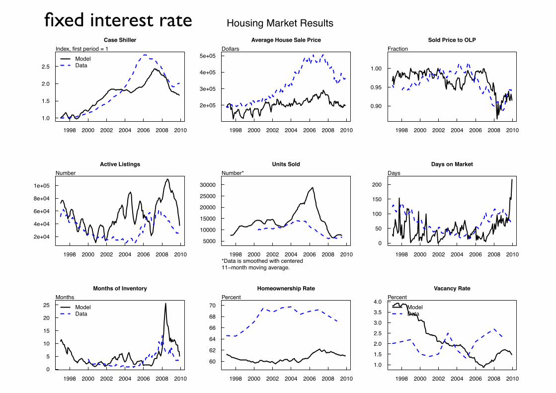
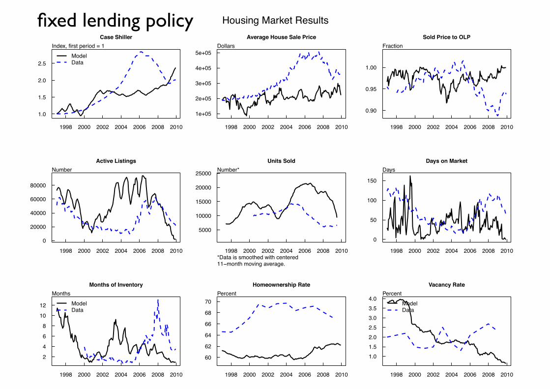
Resultswhenwefiteachmoduleseparatelyondatathatisnotthe
targetdata.
17
Page 18
Case Shiller
1998 2000 2002 2004 2006 2008 2010
1.0
1.5
2.0
2.5
Index, first period = 1ModelData
Average House Sale Price
1998 2000 2002 2004 2006 2008 2010
1e+05
2e+05
3e+05
4e+05
5e+05Dollars
Sold Price to OLP
1998 2000 2002 2004 2006 2008 20100.85
0.90
0.95
1.00
Fraction
Active Listings
1998 2000 2002 2004 2006 2008 2010
20000
40000
60000
80000
100000
120000 NumberUnits Sold
1998 2000 2002 2004 2006 2008 2010
5000
10000
15000
20000
25000
30000Number*
*Data is smoothed with centered11−month moving average.
Days on Market
1998 2000 2002 2004 2006 2008 2010
0
50
100
150
200
250Days
Months of Inventory
1998 2000 2002 2004 2006 2008 201005
101520253035
MonthsModelData
Homeownership Rate
1998 2000 2002 2004 2006 2008 2010
60
62
64
66
68
70Percent
Vacancy Rate
1998 2000 2002 2004 2006 2008 2010
1.0
1.5
2.0
2.5
3.0
3.5
4.0Percent
ModelData
Housing Market ResultsBaseline result
Page 19
Case Shiller
1998 2000 2002 2004 2006 2008 2010
1.0
1.5
2.0
2.5
Index, first period = 1ModelData
Average House Sale Price
1998 2000 2002 2004 2006 2008 2010
2e+05
3e+05
4e+05
5e+05Dollars
Sold Price to OLP
1998 2000 2002 2004 2006 2008 2010
0.90
0.95
1.00
Fraction
Active Listings
1998 2000 2002 2004 2006 2008 2010
2e+04
4e+04
6e+04
8e+04
1e+05
NumberUnits Sold
1998 2000 2002 2004 2006 2008 2010
5000
10000
15000
20000
25000
30000
Number*
*Data is smoothed with centered11−month moving average.
Days on Market
1998 2000 2002 2004 2006 2008 2010
0
50
100
150
200
Days
Months of Inventory
1998 2000 2002 2004 2006 2008 20100
5
10
15
20
25Months
ModelData
Homeownership Rate
1998 2000 2002 2004 2006 2008 2010
60
62
64
66
68
70Percent
Vacancy Rate
1998 2000 2002 2004 2006 2008 2010
1.0
1.5
2.0
2.5
3.0
3.5
4.0Percent
ModelData
Housing Market Resultsfixed interest rate
Page 20
Case Shiller
1998 2000 2002 2004 2006 2008 2010
1.0
1.5
2.0
2.5
Index, first period = 1ModelData
Average House Sale Price
1998 2000 2002 2004 2006 2008 2010
1e+05
2e+05
3e+05
4e+05
5e+05Dollars
Sold Price to OLP
1998 2000 2002 2004 2006 2008 2010
0.90
0.95
1.00
Fraction
Active Listings
1998 2000 2002 2004 2006 2008 2010
0
20000
40000
60000
80000
NumberUnits Sold
1998 2000 2002 2004 2006 2008 2010
5000
10000
15000
20000
25000 Number*
*Data is smoothed with centered11−month moving average.
Days on Market
1998 2000 2002 2004 2006 2008 2010
0
50
100
150
Days
Months of Inventory
1998 2000 2002 2004 2006 2008 2010
2
4
6
8
10
12
MonthsModelData
Homeownership Rate
1998 2000 2002 2004 2006 2008 2010
60
62
64
66
68
70Percent
Vacancy Rate
1998 2000 2002 2004 2006 2008 2010
1.01.52.02.53.03.54.0
PercentModelData
Housing Market Resultsfixed lending policy
Page 21
BankofEnglandmodel(Bap'sta,Farmer,Hinterberger,Low,Tang,Uluc)
• UsedtogiveadvicetotheFinancialPolicyCommieeeonlendingpolicyandforpolicyrela'ngtobuytoletinvestors
• Mainconclusion:Restric'ngdebttoincomera'ocanbeeffec'veindampingbubbles
21
Page 22
Challengeofquan'ta'vesimula'on
• Es'mateparameters• Ini'aliza'on• Valida'on– whatdoesthemodeldowell,whatdoesitdopoorly?
• Aeribu'ngcausality
22
Page 23
Parameteres'ma'on
• UsuallynoclosedformexpressionofABM• DangerofoverfiGng• Typicalmethod:minimizedistancetodata
23
Page 24
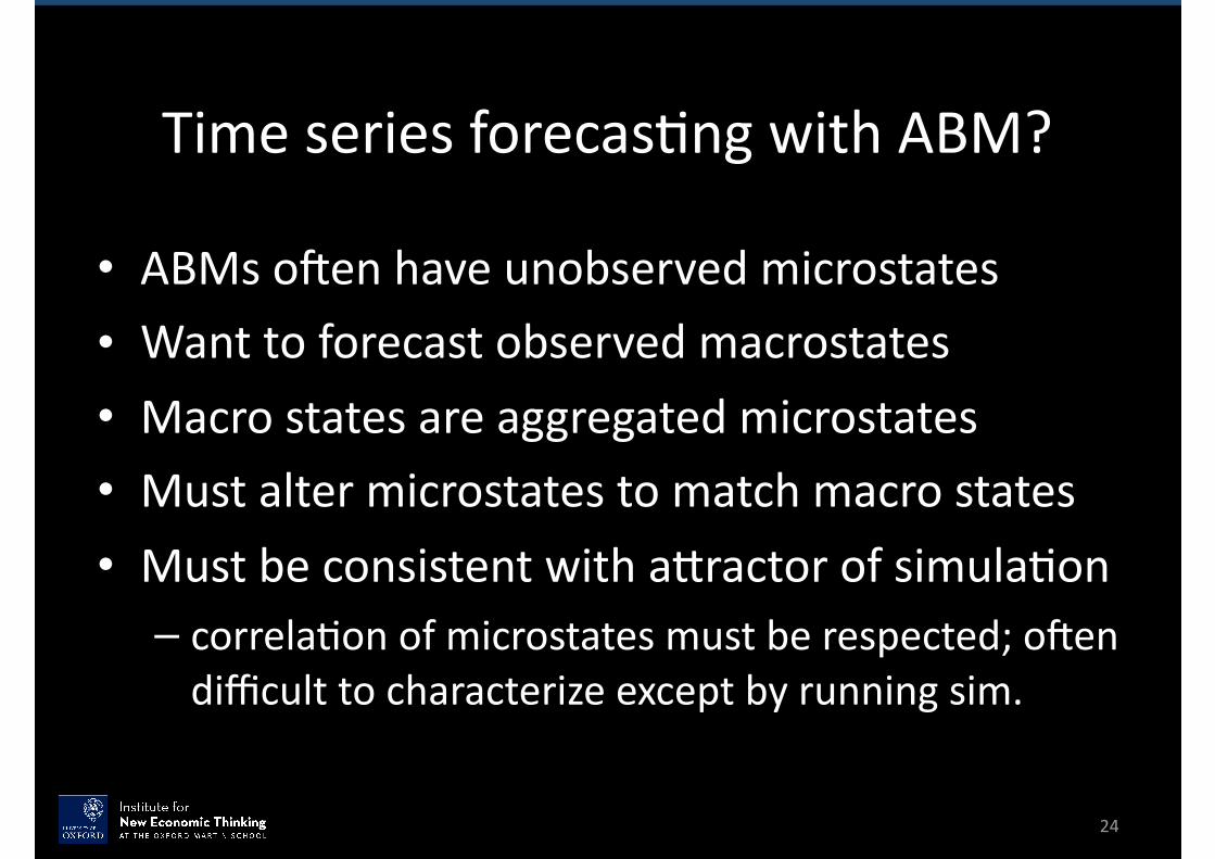
Timeseriesforecas'ngwithABM?
• ABMsoZenhaveunobservedmicrostates• Wanttoforecastobservedmacrostates• Macrostatesareaggregatedmicrostates• Mustaltermicrostatestomatchmacrostates• Mustbeconsistentwithaeractorofsimula'on– correla'onofmicrostatesmustberespected;oZendifficulttocharacterizeexceptbyrunningsim.
24
Page 25
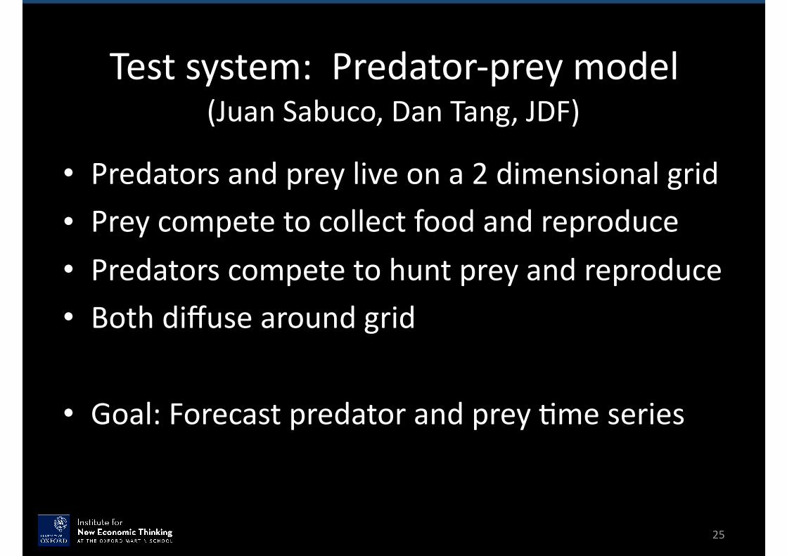
Testsystem:Predator-preymodel(JuanSabuco,DanTang,JDF)
• Predatorsandpreyliveona2dimensionalgrid• Preycompetetocollectfoodandreproduce• Predatorscompetetohuntpreyandreproduce• Bothdiffusearoundgrid
• Goal:Forecastpredatorandprey'meseries
25
Page 26
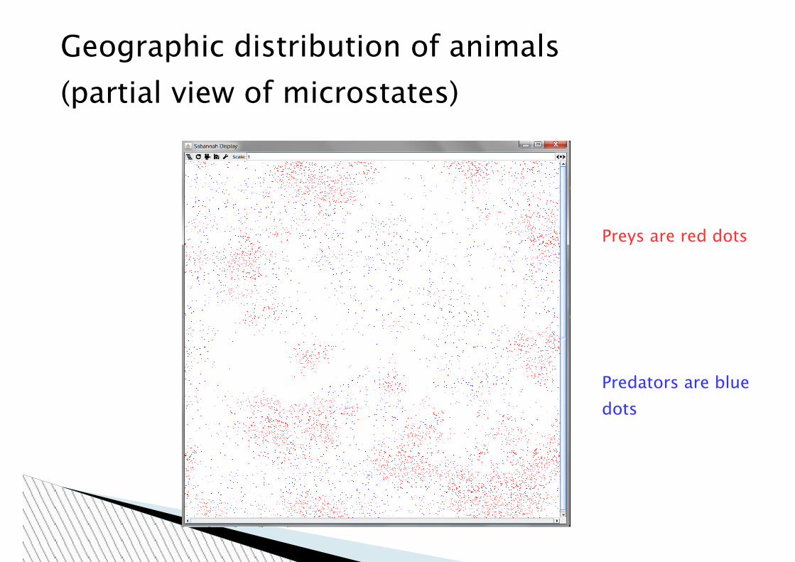
Geographic distribution of animals (partial view of microstates)
Preys are red dots
Predators are blue dots
Page 27
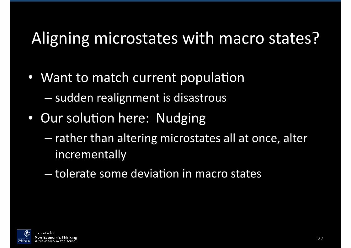
Aligningmicrostateswithmacrostates?
• Wanttomatchcurrentpopula'on– suddenrealignmentisdisastrous
• Oursolu'onhere:Nudging– ratherthanalteringmicrostatesallatonce,alterincrementally
– toleratesomedevia'oninmacrostates
27
Page 28
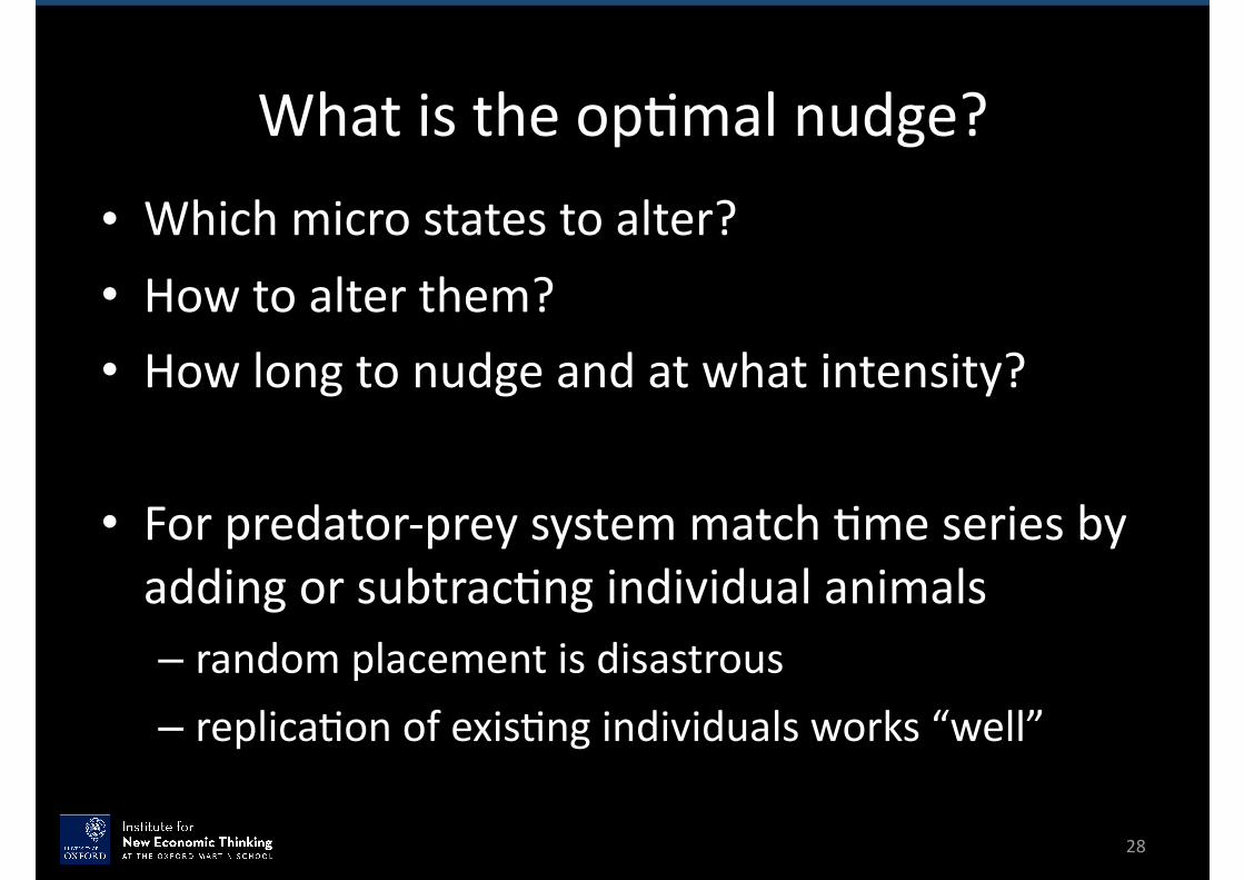
Whatistheop'malnudge?• Whichmicrostatestoalter?• Howtoalterthem?• Howlongtonudgeandatwhatintensity?
• Forpredator-preysystemmatch'meseriesbyaddingorsubtrac'ngindividualanimals– randomplacementisdisastrous– replica'onofexis'ngindividualsworks“well”
28
Page 29
Nudging predator-prey model
x are the predators y are the prey
)(),(1 naprednnn xxKyxfx −−=+
)(),(1 napreysnnn yyKyxgy −−=+
Page 30
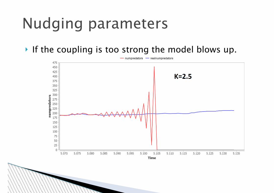
} If the coupling is too strong the model blows up.
Nudging parameters
Page 31
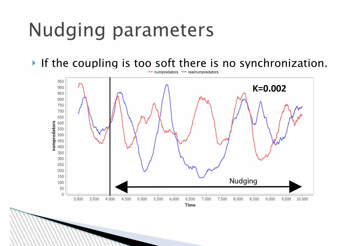
} If the coupling is too soft there is no synchronization.
Nudging parameters
Page 32
} For the right parameters there is synchronization.
Nudging parameters
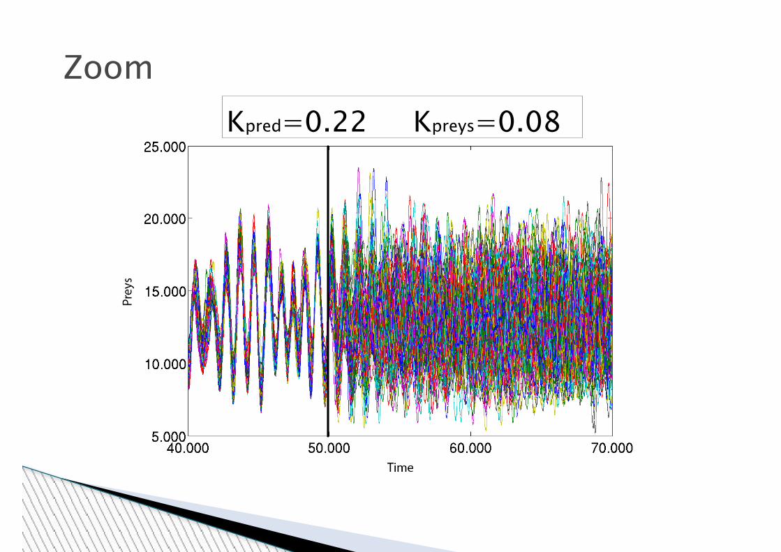
Page 33
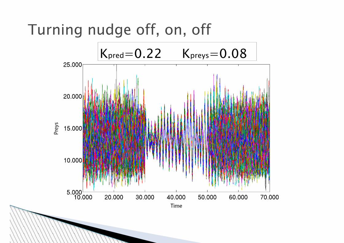
Turning nudge off, on, offKpred=0.22 Kpreys=0.08
Page 34
ZoomKpred=0.22 Kpreys=0.08
Page 35
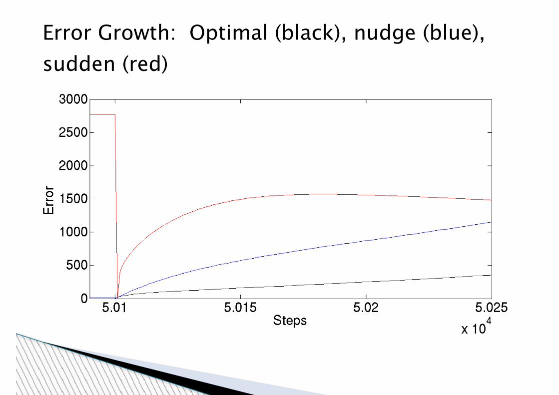
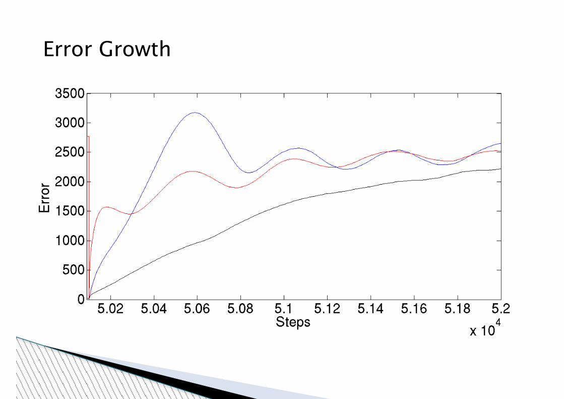
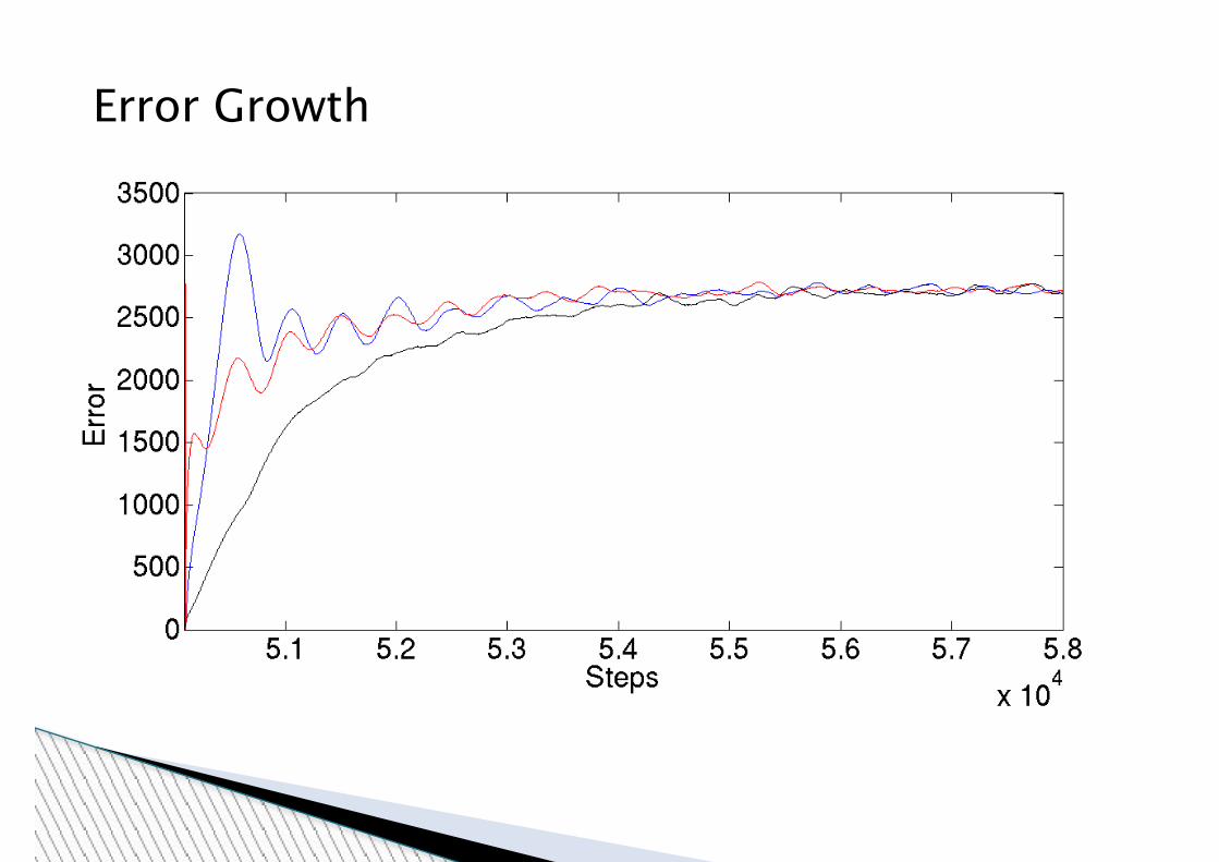
Error Growth: Optimal (black), nudge (blue), sudden (red)
Page 38
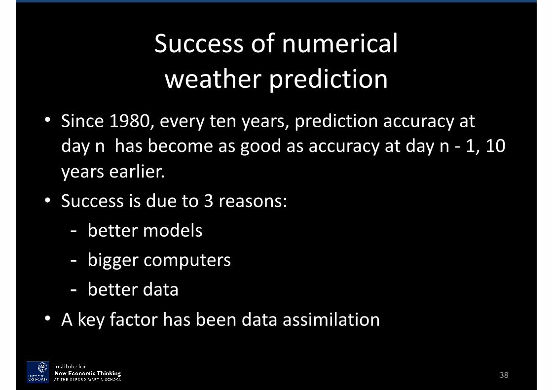
Successofnumericalweatherprediction
• Since1980,everytenyears,predictionaccuracyatdaynhasbecomeasgoodasaccuracyatdayn-1,10yearsearlier.
• Successisdueto3reasons:- bettermodels- biggercomputers- betterdata
• Akeyfactorhasbeendataassimilation
38
Page 40
Predicting chaotic time series
(farmer and Sidorowich, 1987)
E ⇡ Ce(m+1)�1TN�(m+1)/D
Page 41
Closelyrelatedtoproblemsoftimeseriesembedding
41
Page 42
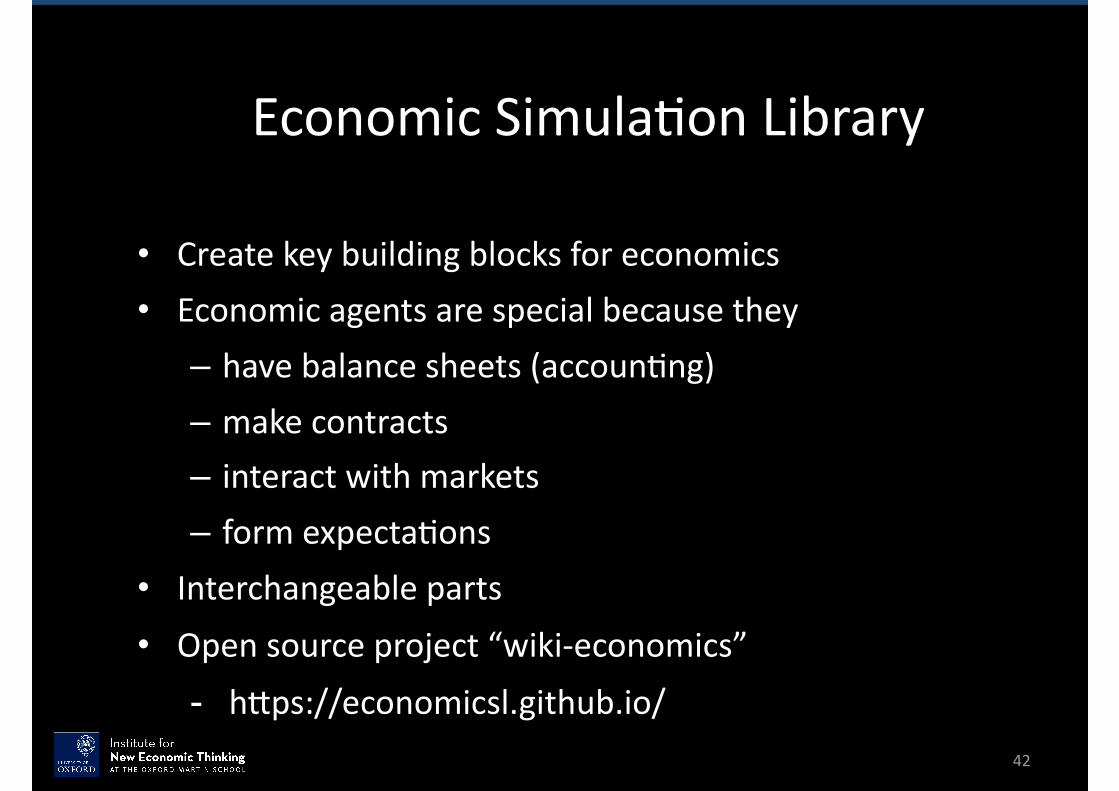
EconomicSimula'onLibrary
• Createkeybuildingblocksforeconomics• Economicagentsarespecialbecausethey– havebalancesheets(accoun'ng)– makecontracts– interactwithmarkets– formexpecta'ons
• Interchangeableparts• Opensourceproject“wiki-economics”- heps://economicsl.github.io/
42
Page 43
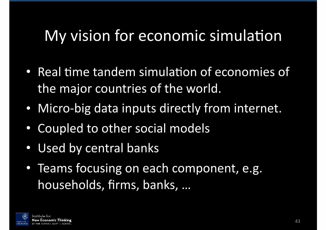
Myvisionforeconomicsimula'on
• Real'metandemsimula'onofeconomiesofthemajorcountriesoftheworld.
• Micro-bigdatainputsdirectlyfrominternet.• Coupledtoothersocialmodels• Usedbycentralbanks• Teamsfocusingoneachcomponent,e.g.households,firms,banks,…
43
Page 44
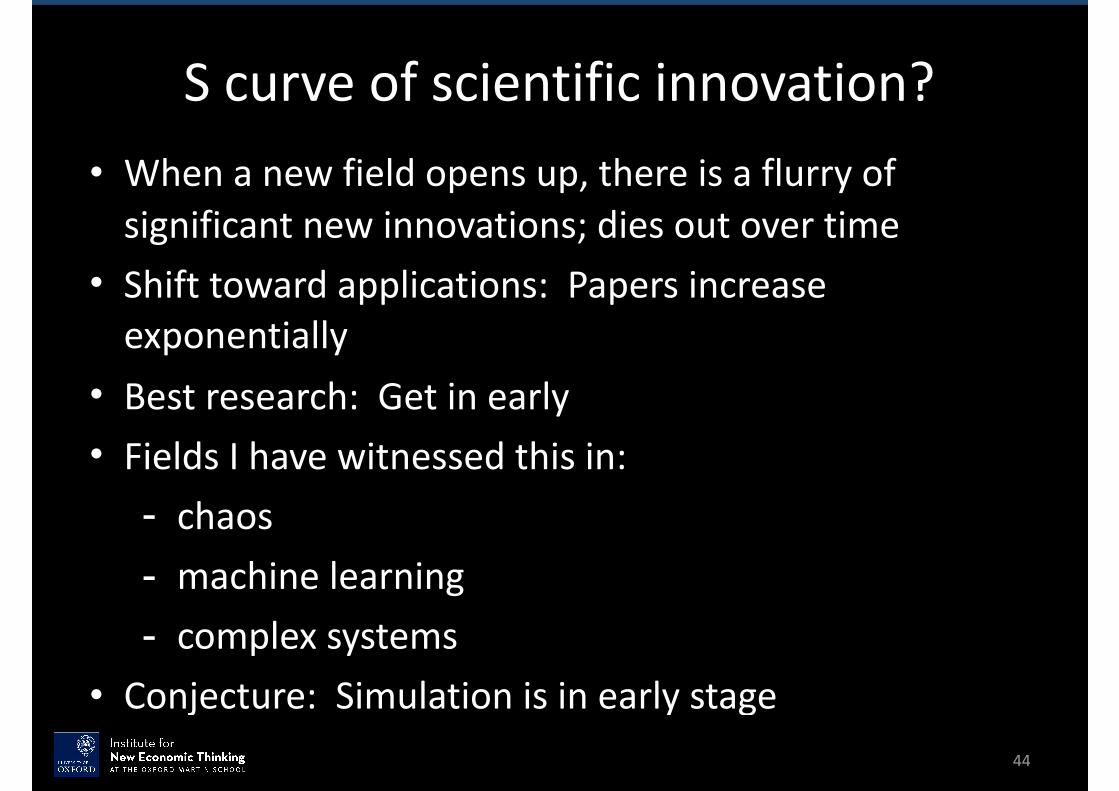
Scurveofscientificinnovation?• Whenanewfieldopensup,thereisaflurryofsignificantnewinnovations;diesoutovertime
• Shifttowardapplications:Papersincreaseexponentially
• Bestresearch:Getinearly• FieldsIhavewitnessedthisin:- chaos- machinelearning- complexsystems
• Conjecture:Simulationisinearlystage44
Page 45
Summary
• Simula'onhasenormousbutsofarlargelyunexploredpoten'al.
• Newwayofdoingeconomics:Don’tneedequilibrium,u'litymaximiza'on,closedform.
45


![- Designing simulaon-based medical educaon and the role of ......to collaborate in providing preventive, curative, rehabilitative and other health-related services.” [20]. The term](https://static.documents.pub/doc/80x56/6097501773ff216914111c70/-designing-simulaon-based-medical-educaon-and-the-role-of-to-collaborate.jpg)


