Simulating Nonlinear Tax Rules and Nonstandard … Simulating Nonlinear Tax Rules and Nonstandard...

This PDF is a selection from an out-of-print volume from the National Bureauof Economic Research

Volume Title: Behavioral Simulation Methods in Tax Policy Analysis

Volume Author/Editor: Martin Feldstein, ed.

Volume Publisher: University of Chicago Press

Volume ISBN: 0-226-24084-3

Volume URL: http://www.nber.org/books/feld83-2

Publication Date: 1983

Chapter Title: Simulating Nonlinear Tax Rules and Nonstandard Behavior:An Application to the Tax Treatment of Charitable Contributions

Chapter Author: Martin S. Feldstein, Lawrence Lindsey

Chapter URL: http://www.nber.org/chapters/c7708

Chapter pages in book: (p. 139 - 172)

5 Simulating Nonlinear Tax Rules and Nonstandard Behavior: An Application to the Tax Treatment of Charitable Contributions Martin Feldstein and Lawrence B. Lindsey

The effect of existing tax rules on charitable contributions has been the subject of several econometric studies in recent years.’ The present paper uses the results of those studies as the basis for examining the potential effects of alternative tax rules that might be applied in extending the charitable deduction to nonitemizers2 Our focus is on the effect that such changes in tax rules would have on charitable contributions, on tax liabilities, and on the distribution of these effects by income class.

Our methodological emphasis is on simulating behavioral responses to nonlinear tax rules, e.g. a rule that allows nonitemizers to deduct charitable gifts in excess of $300 per year. We examine three types of response to such nonlinear rules. The first is based on conventional demand analysis with a nonlinear budget constraint. The second recognizes that individuals have an incentive to respond to a floor by “bunching” their

Martin Feldstein is professor of economics, Harvard University (on leave). He was formerly president of the National Bureau of Economic Research and is currently chair- man, Council of Economic Advisers.

Lawrence B. Lindsey is tax economist at the Council of Economic Advisers. He is on leave from Harvard University and the National Bureau of Economic Research.

The authors are grateful to the members of the Tax Simulation Project and especially to Daniel Feenberg and Daniel Frisch for helpful discussions, to the NBER and National Science Foundation for support of this research, and to Harvey Galper for valuable comments on the previous version. The views expressed here are the authors’ and should not be attributed to any organization.

1. See Boskin and Feldstein (1977), Clotfelter (1980), Clotfelter and Steuerle (1979), Feldstein (1975a,b), Feldstein and Clotfelter (1976), Feldstein and Taylor (1976).

2. A variety of proposals to extend the charitable deduction have been made over the years, especially in conjunction with tax change proposals that would reduce the fraction of taxpayers itemizing their personal deductions. One recent proposal is contained in the bill introduced in the House of Representatives by Congressmen Fisher, Moynihan, and Packwood ( S . 219,96th Congress, 2d session). For a copy of the bill and further analysis, see “Hearings before the Subcommittee on Taxation and Debt Management generally and the Committee on Finance, United States Senate, January 30 and 31, 1980.” 139

140 Martin FeldsteidLawrence B. Lindsey

contributions over time, e.g. by contributing only in alternate years to reduce the fraction of total contributions that are below the floor and therefore that do not receive the tax benefit. The third approach departs from the usual utility maximization model of demand to consider a quite different type of altruistic behavior that may be appropriate for studying charitable contributions. The essential feature of this approach is that it assumes each individual wishes to make charitable gifts with some fixed net-of-tax cost; changes in tax rules alter the gross amount of giving to maintain this net cost.

All three approaches are generally consistent with the available statistical evidence. The behavior of taxpayers under existing rules does not allow a choice among the three models; in statistical terms, the model is underidentified. This underidentification does not affect predictions of the effects of alternative linear tax rules, e.g. substituting a credit for the existing deduction. Although the predicted effects of an alternative linear tax rule do not depend on which of the three models is assumed to be ~ o r r e c t , ~ with nonlinear tax rules the three models can have very different implications. Predictions of the effects of nonlinear tax rules must therefore be regarded as conditional on the model specification, and any user of our analysis must “weight” these conditional predictions by his own subjective probabilities of the appropriateness of the model.

The simulations are all made with the National Bureau of Economic Research TAXSIM model. This computerized model, like the one used by the Treasury and the Joint Committee on Taxation, bases its calculations on the large stratified random sample of individual tax returns that are provided for this purpose by the Internal Revenue Service. But unlike these other models, the NBER TAXSIM model is specifically designed to take into account the response of taxpayer behavior to changes in tax rules.‘ The version of the model used in the present paper is based on the tax law for 1977 and uses a sample of 23,111 individual tax returns for that year.’

The first section of the paper summarizes the previous econometric evidence on charitable giving that forms the basis for the parameter values used in the current simulations. Section 5.2 describes the alternative tax rules and the three models of behavior that will be simulated. Some technical aspects of the simulation procedure, including the imputation of contributions to nonitemizers and the calculation of the effective cost of charitable gifts, are discussed in section 5.3. The simulation results are presented in sections 5.4 and 5.5. There is a brief concluding section.

3. The choice between the third model and the first two does have some effect on the

4. The economists who have participated in the development of the TAXSIM model are

5. These 23,111 returns are a random 25% sample of the 1977 Treasury Tax Model

estimated response to changes in tax rules, but the size of the effect is relatively small.

Daniel Feenberg, Martin Feldstein, Daniel Frisch, Larry Lindsey, and Harvey Rosen.

Public Use Sample.

141 Simulating Nonlinear Tax Rules and Nonstandard Behavior

5.1 Econometric Evidence on Charitable Giving

Since this paper will not present any new econometric evidence on charitable giving, it is useful to review the previous research. The current tax law allows any taxpayer who itemizes his deductions to subtract the value of charitable contributions in calculating taxable income. The “price” of one dollar’s contribution to a charitable organization in terms of the foregone disposable income of the donor therefore varies inversely with his marginal tax rate. Of course, for anyone who does not itemize his deductions, the price of one dollar’s contribution is one dollar of foregone disposable income.6

The key parameter that determines the effect of the existing charitable deduction and of alternative linear tax rules is the price elasticity, i.e. the elasticity of the individual’s gross (pretax) charitable gift with respect to the price of giving. The appropriate value is of course the partial elasticity, holding constant the level of income and such other demographic characteristics that might be associated with the price. Several studies in recent years, based on quite different bodies of data, have concluded that the price elasticity of giving is between - 1.0 and - 1.5. There is a striking degree of consistency and relative precision in these estimates even though they are based on different years and different types of data.

Feldstein (1975a, b) used the data published by the Internal Revenue Service on the mean level of charitable giving and the mean level of disposable income in each of twenty-seven adjusted gross income (AGI) classes for the alternate years between 1948 and 1968. These data refer only to individuals who itemized their deductions. A constant elasticity specification was estimated:

(1) In Gi, = bo + bl In P,, + b, In Y,, + ei, , where Ci, is the mean charitable gift of individuals in AGI class i in year t , P,, is the price calculated at the mean taxable income in that class, and Y,, is the mean disposable income in that class. The changing tax rates as well as the differences in the rates among classes were used to estimate the price elasticity. The basic estimate in this study, with the sample re- stricted to taxpayers whose AGIs were between $4,000 and $100,000 at 1967 prices, was - 1.24 with a standard error of 0.10. Including all income classes in the sample raised the elasticity to - 1.46 with a standard error of 0.08.

Feldstein and Clotfelter (1976) used individual household data collected by the Census Bureau in 1963 and 1964 for the Federal Reserve Board’s Survey of Financial Characteristics of Consumers. Their sample of 1,406 individuals provided information on wealth and demographic

6. This ignores the special problem of gifts of appreciated property, a subject to which we return later.

142 Martin Feldstein/Lawrence B. Lindsey

characteristics as well as on income and charitable giving. The data made it possible to estimate for each household the price of charitable giving and a measure of disposable income defined as the total income received minus an estimate of the tax that would be due if no contribution were made. The basic price elasticity estimate in this study was - 1.15 (standard error 0.20). Several variants of the basic equation showed that the estimated price elasticity was not sensitive to the measurement of permanent income or the inclusion of a variety of other demographic and economic characteristics.

Feldstein and Taylor (1976) used a similar specification to study a sample of more than 15,000 taxpayers who itemized their deductions and whose tax returns were included in the 1970 Treasury Tax File, a stratified random sample of individual tax returns. The basic price elasticity estimate was - 1.29 (standard error 0.06). Repeating this calculation for the 1962 Treasury Tax File data showed a price elasticity of - 1.09 (standard error 0.03). A price elasticity estimate based on the change in the tax schedule between 1962 and 1970 was - 1.39 (standard error 0.19).

Similar estimates were obtained in several other studies using different sets of microeconomic data. Reece (1979) used the 1972-73 Consumer Expenditure Survey of the Bureau of Labor Statistics and estimated a price elasticity of - 1.19 using a Tobit procedure. Dye (1977) studied 1974 University of Michigan Survey Research Center data on households with incomes under $50,000 and estimated a price elasticity of - 2.25. Clotfelter and Steuerle (1979), using tax data for 1975, estimated a price elasticity of - 1.25. And Clotfelter (1980), using the unstratified random sample of tax returns for 1972, obtained a price elasticity of - 1.40.

These estimates refer to the entire population or to all taxpayers who itemized and not to any particular income class. The present analysis of the potential effect of extending the charitable deduction to those who do not currently itemize their deductions makes it particularly important to have an estimated price elasticity for middle and lower income households; more than 90% of 1977 nonitemizers had adjusted gross income of less than $20,000. Although separate estimates for each income class cannot be made as precisely as for the sample as a whole, the evidence generally indicates that the relevant elasticity for this group is as high as for the population as a whole.

The pooled data by year and income class (Feldstein 1975a,b) were analyzed in separate regressions for different income groups. For the sixty-four observations with mean real income (in 1967 dollars) between $4,000 and $10,000, the estimated price elasticity was - 1.80 (standard error 0.56). Among taxpayers with real incomes between $10,000 and $20,000, the corresponding estimate was - 1.04 (standard error 0.76, with twenty-seven observations).


Despite the small samples, these data had the advantage of tax sched- ules that varied over time. When attention is limited to a single cross section of individual data, it is more difficult to estimate separate equations in each income class. This is particularly true in the low and middle income classes, where there is a very high correlation between income and tax rates.’ It is nevertheless possible to allow the estimated price elasticity to vary with income or marginal tax rate while estimating the other parameters from the entire sample.

The Feldstein and Clotfelter (1976) study found that the price elasticity was greatest for those with the highest “price of giving”; the estimated elasticity was - 1.82 (s.e. 0.64) for those with a price of giving in excess of 0.7 and then fell to - 1.26 (s.e. 0.42) for those with a price between 0.3 and 0.7 and to - 1.16 (s.e. 0.20) for those with a price below 0.3. The differences are not statistically significant but, if anything, provide evidence that the current nonitemizing population has a higher elasticity.

The Feldstein and Taylor (1976) study had a much larger sample and could therefore obtain estimates with smaller standard errors. The estimated price elasticities varied inversely with income, from - 2.26 (s.e. 0.42) for taxpayers with incomes below $10,000 and - 1.82 (s.e. 0.24) for taxpayers with incomes between $10,000 and $20,000 to - 1.17 (s.e. 0.09) for those with incomes between $50,000 and $100,000 and - 1.27 (s.e. 0.06) for those with incomes over $100,000. An analogous equation for 1962 is not reported. Estimates of separate price and income elasticities in each income class give implausible values for the lowest income class (those with AGI between $4,000 and $20,000): - 3.67 (s.e. 0.45) for 1962 and - 0.35 (s.e. 0.52) for 1970.

In a separate study designed to measure the price elasticity for the lower and middle income groups, Boskin and Feldstein (1977) used survey data collected in 1974 by the University of Michigan Survey Research Center on households with incomes below $30,000. Because these are survey data rather than tax return data, they contain information on contributions by nonitemizers as well as itemizers. This provides much more price variation at each income level. The Boskin-Feldstein analysis estimated a price elasticity of - 2.54 (s.e. 0.28) for this group. An additional analysis of these data showed that the difference between itemizers and nonitemizers could be explained completely by the price effect without recourse to a separate “itemization” effect.

Clotfelter and Steuerle (1979) estimated a variety of different specifications for separate income classes using the Treasury Tax Model for 1975. They found that the estimated results in the lower income class were quite

7. In higher income classes, there is much more variation in tax rates at each level of adjusted gross income as well as substantial income variation within tax brackets.


sensitive to the particular specification. The basic logarithmic equation implied price elasticities of - 0.9 for incomes of $4,000 to $10,000 and - 1.3 for incomes of $10,000 to $20,000. Estimating a single equation for all income classes but using a more general functional form implied lower price elasticities; the estimates ranged between - 0.4 and - 0.7. But constraining the coefficient to be the same for all income classes reverses this effect and implies price elasticities of - 2.2 and - 1.4. In our view, this sensitivity shows the difficulty of trying to infer separate elasticities for low and middle income groups.

Before turning to the simulations, it is useful to consider the plausibil- ity of a price elasticity between 1 and 2 for a typical nonitemizing family. In 1977, families with adjusted gross incomes between $10,000 and $15,000 who itemized their deductions gave an average of $522. If such a family had a taxable income of $8,000, the price per dollar of giving would be approximately 80 cents. A price elasticity of - 1 .O and a price of 0.80 imply that deductibility raises giving by 25%, i.e. by $104 from $418 to $522. Similarly, a price elasticity of - 2.0 implies that deductibility raised giving by 56%, or by $188 from $334 to $522. Changes of this magnitude are not contrary to intuition or to any other evidence.

To be conservative, the estimates developed in this paper will generally be based on a price elasticity of - 1.3. Some additional estimates using price elasticities of - 0.7, - 1.0, and - 1.6 will also be presented.

5.2 Extending the Contribution Deduction to Nonitemizers

The basic proposal to be analyzed in this paper allows all taxpayers to deduct charitable contributions in the calculation of taxable income. More specifically, taxpayers who itemize other deductions would continue to include charitable contributions as part of their deductions. Taxpayers who do not itemize other deductions would be allowed to subtract their charitable contribution from gross income in the same way that they now subtract an amount for each exemption. In this way, there is no change in adjusted gross income or in any of the amounts that depend on it.

This basic scheme might be modified by limiting the charitable deduction of nonitemizers to the excess over some dollar amount or some percentage of the taxpayer’s adjusted gross income. A rationale for such a “floor” is that the standard deduction implicitly recognizes some minimal or typical charitable gift so that individuals should get an explicit deduction only for the excess over that amount.S An alternative rationale

8. The logic of that argument is hardly compelling. If the charitable deduction is extended nonitemizers, it would be more appropriate to reduce the standard deduction by the currently assumed amount of the “typical” gift and then allow all individuals the full amount of their deduction.


for a floor is that it can reduce the loss of tax revenue and, to the extent that contributions exceed the floor amount, the reduction in revenue loss would have no impact on the marginal incentive to give. For example, in 1977 taxpayers with AGIs between $15,000 and $20,000 who did not itemize made charitable gifts averaging nearly $400. For someone giving an average amount, a $300 floor would have no effect at the margin on the incentive to give. The current paper analyzes two alternative floors: the first is $300, and the alternative is 3% of AGI.

5.2.1 The Conventional Demand Model The effects of extending the charitable deduction to nonitemizers, and

particularly the effects of the floors, depend on the type of individual behavior that is assumed. The most basic behavioral assumption, and the one that underlies the specification of the econometrically estimated equations, is that individual giving responds to a change in price according to the constant elasticity formula:

where GI is the level of annual giving after the “reform,” Go is the level of annual giving before the reform,y Po is the price before the reform,’O PI is the price after the reform, and a is the price elasticity of demand. There is no need to adjust separately for the change in disposable income since the estimated price elasticity includes the income effect as well as the sub- stitution effect; i.e. the initial econometric equation defines the disposable income as AGI minus the tax that would be due if the individual made no charitable contribution.

More specifically, equation (2.2) describes what is essentially the response of nonitemizers (i.e. those who under existing law are nonitemizers) when they are allowed to deduct charitable gifts. For most itemizers, the proposal involves no change in behavior. However, about 6% of current itemizers would cease to itemize if they could then deduct their charitable contributions; i.e. their itemized deductions excluding charitable contributions are less than the standard deduction to which they would be entitled.’l For most of these “switchers” there is no change in marginal tax rate and therefore no change in price. However, since an individual switches only if his tax bill is reduced, there is a small income

9. The method of imputing an initial level of giving for nonitemizers is discussed in section 5.3 of this paper.

10. For nonitemizers, Po differs from 1 only because of gifts of appreciated property. This difference is discussed in section 5.3. Although as a practical matter the difference from 1 for this group is small enough to ignore completely, our price calculations do reflect for each individual the average percentage of appreciated property in total contributions.

11. In 1977, the standard deduction was $3,200 for a married couple and $2,200 for a single individual.


effect. The giving of a switcher can be calculated according to the equation

(2.2) where Yo is the initial value of total income minus the tax liability if the individual makes no contribution and Y, is the corresponding value if the individual stops itemizing and uses the standard deduction.’2 The difference between Yl and Yo is the tax that the individual saves by switching from itemizing to using the standard deduction, given that the charitable contribution is deductible in any case.

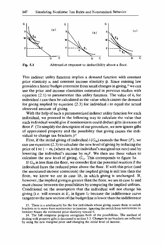
Although the demand behavior implied by equation (2.1) is adequate for estimation and for simulating alternative linear budget constraints, it is inadequate for analyzing alternative nonlinear budget constraints. Figure 5.1 illustrates the nature of this problem in a simple case. The standard deductor initially faces a budget line UVW with a slope of - 1 between giving (G) and other spending (C). He chooses point El . Allow- ing standard deductors to take an additional deduction for charitable gifts above a floor ( F ) puts a kink in the budget line which becomes UVX.

In the case shown in figure la , the individual was giving more than the floor even without the deduction. For such an individual, the deductibility with a floor is equivalent to an ordinary price change except for an offsetting negative income effect equal to mF, where m is the individual’s marginal tax rate. This case could therefore be analyzed using the demand function of equation (2.2) with appropriate definitions of PI and Y 1 .

In the case shown in figure lb , the individual was giving less than the floor. The change in the budget constraint therefore occurs in an irrelevant section of the budget constraint and the individual continues to give at E l . This could also be analyzed using the demand function, since the price is unchanged for this individual.

But the choice in figure l c cannot be analyzed with the demand function. The individual initially gives an amount less than the floor F. But the individual’s indifference curve cuts the new branch of the budget constraint, implying that the individual’s optimum point is on the new branch. This can only be determined by an explicit utility comparison.

In order to be able to deal with situations like figure lc, we therefore continue the analysis with the help of an explicit utility function that implies the constant elasticity demand structure of equation (2.2). We follow Hausman (1979) and write the indirect utility function of individual i as

GI = Go(Pi/Po)*( YI/Yo)’ ,

y’ - P

l + a 1 - p vt ( p , y ) = - kip= + -

12. An income elasticity of 0.7 is used in the calculations; see Feldstein and Taylor (1976) for supporting evidence. Because the relevant income changes are always very small, the results are very insensitive to the choice of this elasticity.


Fig. 5.1 Alternative response to deductibility above a floor.

This indirect utility function implies a demand function with constant price elasticity (Y and constant income elasticity p. Since existing law provides a linear budget constraint from small changes in giving,13 we can use the price and income elasticities estimated in previous studies with equation (2.1) to parameterize this utility function. The value of ki for individual i can then be calculated as the value which causes the demand for giving implied by equation (2.3) for individual i to equal the actual observed amount of giving.

With the help of such a parameterized indirect utility function for each individual, we proceed in the following way to calculate the value that each individual would give if nonitemizers could deduct gifts in excess of floor F. (To simplify the description of our procedure, we now ignore gifts of appreciated property and the possibility that giving causes the individual to change tax bracket^.)'^

First, if the initial giving of individual i (Goi) exceeds the floor ( F ) , we can use equation (2.3) to calculate the new level of giving by reducing the price of 1 to 1 - mi (where mi is the individual’s marginal tax rate) and by lowering the individual’s income by miF. We then use these values to calculate the new level of giving, Gli. This corresponds to figure la .

If Goi is less than the floor, we consider first the potential reaction if the individual faces the reduced price above the floor. If with this price (and the associated income correction) the implied giving is still less than the floor, we know we are in case lb , in which giving is unchanged. If, however, the implied giving is greater than the floor, we are in case l c and must choose between the possibilities by comparing the implied utilities. Conditional on the assumption that the individual will not change his giving (i.e. will remain at El in figure l c because the indifference curve tangent to the new section of the budget line is lower than the indifference

13. There is a nonlinearity for the few individuals whose giving causes them to switch brackets or to move from nonitemizer to itemizer. Ignoring the switch from nonitemizer to iternizer biases the estimated price elasticity toward 0.

14. The full computer program recognizes both of the possibilities. The method of dealing with property gifts is discussed in section 5.3. Changes in tax brackets are reflected by using the new marginal price and changing the initial level of income.


curve tangent at E l ) , we evaluate the utility at the initial price (pi = 1)15 and unchanged income, say Voi. Then, conditional on the assumption that the individual increases his giving (i.e. moves to point E2 in figure lc), we take pi to be the itemized price (8 = 1 - mi, except for gifts of appreciated property) and reduce income by mjF. This implies an increased value of giving Gli and an associated utility value Vlj . The choice between the two points is then made by comparing Voi and VIi for the individual.

An analogous calculation is used to analyze the possibility that an individual who is currently an itemizer might switch to using the standard deduction if he could continue to itemize his charitable gifts. To decide whether to switch, the individual compares his utility level as an itemizer with the utility level that he would achieve as a nonitemizer who can deduct his charitable giving. In practice, about 6% of current itemizers would find that it is desirable to use the standard deductions when charitable gifts become eligible for a separate deduction.

5.2.2 The Bunching of Gifts The use of a floor provides an incentive for individuals to “bunch” their

charitable giving. With a $300 floor, a nonitemizer who gives $300 each year would get no tax reduction. By giving $600 every other year, the individual would also have a $300 tax deduction every other year, or a 50 cent deduction per dollar of contribution. And by giving $900 every third year, the deduction would rise to 67 cents per dollar of gift. Although the ‘‘logical’’ extreme is of course implausible because of the resulting effect on the individuals’ marginal tax rates and because individuals and institu- tions both have reasons to favor a steady flow of giving, the presence of a floor seems very likely to lead to some bunching.

There is, unfortunately, no experience with charitable deduction floors that can be used to estimate their likely effect on bunching. We have, however, constructed two alternative simulation models and tested the parametric sensitivity of the results.

Both models assume that the extent of bunching depends on the potential tax saving from bunching and therefore on both the size of the contribution and the individual’s marginal tax rate. In both models the possibility of bunching is limited to a two-year cycle. The first model assumes that each individual bunches either all of his contributions or none. That is, if he is a “buncher,” he gives only in alternate years. The probability of being a buncher depends on the tax incentive. The second model assumes that everyone is a “partial buncher”; some fraction of his total giving is bunched (i.e. given only in alternate years) while the rest of

15. In the actual calculations,p, is lower than 1 because of gifts of appreciated property.


his contribution is given every year. We will now describe these models as they apply to someone who is currently a nonitemizer.I6

The tax incentive to bunch is a function of the relative cost of giving with and without bunching. Let G l i be the amount that individual i (a nonitemizing taxpayer) would give if charitable gifts in excess of a floor could be deducted.” Let CGli be the net cost to individual i of making this charitable gift in a single year, i.e. without bunching. CGli is equal to G l j reduced by the tax saving associated with the contribution, i.e. the tax saving that results from deducting the excess of G l j over the floor. Similarly, let BCGlj be the net cost of making this charitable gift by bunching two years’ gifts into a single year.lS We assume that the propen- sity to bunch depends on the ratio of these net costs: BCGICG.

More specifically, the first model assumes that the probability that individual i will bunch is given by

(2.4) PROBj = 1 - (BCGli/CG$

with p>O. Note that under current law, with no floor, there is no incentive to bunch:I9 BCG = CG and PROB = 0. However, a floor on the charitable deductions implies BCG < CG and therefore PROB > 0. The greater the value of p, the more sensitive the probability of bunching to the relative cost. To appreciate the order of magnitude of this effect, consider a taxpayer who would contribute $400 without bunching ( G l j = 400) and whose marginal tax rate is 30%. With a $300 floor, the cost of giving is $370 with no bunching and $325 with bunching. Thus PROB = 1 - (325/370)” = 1 - (0.88)p. If p = 2, PROB = 0.23, while p = 0.5 implies PROB = 0.06 and p = 10 implies PROB = 0.73. Since econometric evidence about p is unavailable, the simulations show the sensitivity of the conclusions to alternative values of p.

Of course, those individuals who bunch change the amount of their gift because of bunching. If without bunching the individual’s gift is below the floor while bunching makes the gift (in the year in which it is given) greater than the floor, there is a reduction in the price of giving and therefore an incentive to give more. Among those whose gift would be

16. For itemizers, the possibility of switching is again evaluated by comparing the tax liability as an itemizer with the tax liability as a nonitemizer, but this time including the effect of bunching.

17. The calculation of Gli was described in section 5.2.1. 18. This is calculated by finding the tax reduction associated with contributing 2G1,, i .e.

the tax saving that results from deducting the excess of 2G1, over the floor, and then subtracting half of this tax saving from GI,.

19. This assumes that the individual cannot predict year-to-year changes in his marginal tax rate. In fact, there is some predictable variation and therefore some incentive to bunch. Although we believe this is likely to be small, some investigation with the longitudinal tax rule would be worthwhile.


above the floor without bunching, bunching has a positive income effect on the amount of the gift.

In general, a floor reduces the loss of tax revenue that results from extending the deduction to nonitemizers and also reduces the incentive to give associated with such an extension. Bunching increases the revenue loss but, even in the case of complete bunching, still leaves a smaller revenue loss than with no floor. However, even with bunching the incentive to give is not as great as without a floor. Whether the floor raises or lowers the tax-revenue “loss” per dollar of induced extra giving is an empirical question that we will examine in section 5.5 with the help of the simulations.

The alternative “partial bunching” model assumes that all taxpayers bunch some of their giving if there is a floor and that the extent of bunching depends on the cost ratio BCGICG. The idea of partial bunching is based on the asymmetry of information between donors and donees. Much giving is done in response to requests for contributions and is done in such a way that the donee organization and others know the amount of the donor’s gift. The individual who responds to a request for a contribution by saying “I give every other year and this is my off year” may not be credible. Individuals may also prefer to appear more gener- ous, especially for relatively small amounts, by appearing to ignore tax considerations. And making a contribution may seem better than trying to explain the tax law to the sellers of Girl Scout cookies or Little League decals.

We assume that the specific incentive to partial bunching is of the same form as equation (2.4):

(2.5) PROBi = 1 - (BCGlj/CGl;)P ,

where PROBi is the proportion of the charitable gift that individual i bunches. The amounts of the gifts in the ‘‘low’’ and “high” giving years depend on the interaction between bunching, floors, and tax saving. For example, if (1 - PROBi)Gli is greater than the floor, bunching does not change the price of giving in either year but does have an income effect that raises giving to (say) GZi. In this case, the individual gives (1 - PROBj)G2i in the low year and (1 + PROBi)G2; in the high year. Alternatively, if Glj is less than the floor but (1 + PROBi)Gli exceeds the floor, there are both price and income effects in the “high” year but only an income effect in the ‘‘low’’ year. We assume that in the “high” year the individual in this case gives

(1 + P R O B , ) G ~ , ( P ~ / P , ) ~ ( Y ~ / Y ~ J ~ ,

where P, reflects the marginal deductibility and Y1 differs from Yo because of the effects of the floor (which lowers y,) and the bunching (which raises Y1) . Although the income-effect adjustments are not pre-


cise, they are relatively small and further elaborations or refinements have no significant effects.*’

There is one further aspect of the partial bunching model that deserves comment. In the case in which giving without bunching substantially exceeds the floor, the equation that describes partial bunching might still leave giving in both years at levels above the floor. Since in that case there is no gain from bunching, we assume that the proportion bunched is actually zero.

The difference between the effects of the two models of bunching depends on the taxpayer’s initial situation. There are cases in which partial bunching would save no tax and have no effect on giving while total bunching would do both. There are other cases in which partial bunching would have a larger total effect on both giving and tax receipts. The net balance is examined in section 5.5 with the help of the simulations.

5.2.3 Net Altruism Although charitable giving can be modeled like other types of con-

sumer spending, it is worth considering the possibility that charitable behavior is actually “different.” Individuals may make charitable gifts because of a sense of responsibility, religious devotion, altruism, guilt, or other considerations that may cause behavior to differ from traditional utility maximization. We emphasize may because, even with these motivations, actual charitable giving might behave just as traditional theory predicts. Certainly the normal price and income elasticities found in the econometric studies are consistent with this.

But individuals might think about charitable giving in terms of their desire to “sacrifice” or to contribute their “fair share” rather than in terms of the benefits that they can achieve for the donee organization. In this case the deductibility of charitable gifts has the effect of reducing the donor’s “sacrifice” or “net contribution.” To achieve the initial level of sacrifice, the donor must increase the size of his contribution. If the individual wishes to make a fixed sacrifice regardless of the tax law, full deductibility (with no floor) causes the individual to behave as if he had a price elasticity of - 1; that is, G1 = Go( PIIPo) - since this implies a constant net cost of giving, PIGl = POGO.

Although the econometric evidence suggests that the price elasticity is absolutely larger than 1, the possibility of a price elasticity of - 1 cannot be ruled out. If the observed price elasticity were - 1, the available evidence could not be used to distinguish between the traditional demand model and the alternative “net sacrifice” or “net altruism” model. With no floor, the two models are observationally equivalent.

20. See footnote 15.

152 Martin Feldstein /Lawrence B. Lindsey

The presence of a floor causes a substantial difference between the conventional demand model (with a price elasticity of - 1) and the “net altruism” model. Consider an individual who, with no deductibility, contributes $400 and whose marginal tax rate is 30%. The net cost to such an individual is $400. Allowing deductibility with no floor causes the contribution to rise to 400(0.7) - = 571 dollars. With a $300 floor, the conventional model predicts that giving will fall short of $571 only because of a small income effect; the extra tax of $90 caused by the floor would reduce giving by about $5. But the $300 floor implies that the “net altruist” must give substantially less than $571 to maintain the original $400 net cost. In particular, a total gift of $443 would have a net cost of $400.

The possibility that individuals decide on the basis of total net cost rather than marginal net cost implies that a floor does not reduce the loss in tax revenue per dollar of induced additional giving. In the example of the previous paragraph, deductibility with no floor would cause giving to rise by $171 and tax revenue to fall by $171 (0.3 x 571). Deductibility with a $300 floor would cause giving to rise by $43 and tax revenue to fall by $43 (0.3 x 143).

The implications of the “net altruism” model will be considered as part of the simulations in section 5.5.

5.3 Some Technical Aspects of the Simulation Procedure

As we noted in the introduction to this paper, our simulations use the NBER TAXSIM model with the 1977 tax law. Our sample of 23,111 returns is a one-in-four random sample from the Treasury’s Public Use File of 1977 tax returns. In simulating the effect of any tax change proposal, we use the model to calculate consistent values for each individual of the price of giving under the new law, the amount that that individual gives, and the individual’s new tax liability. The entire TAXSIM model with all features of the tax code are used in these calculations. By using the sampling weights provided by the Treasury, we can then aggregate the individual changes in giving and in tax liabilities to obtain estimates for all taxpayers and for taxpayers in each income class.

Two technical issues in the simulation deserve special attention: (1) the calculation of the price of giving, and (2) the estimation of the initial level of giving of nonitemizers.

5.3.1 The Price of Giving The price of giving is defined as the net cost to the taxpayer of a

marginal increase in the charitable contribution. In the simple case of full deductibility, there would be a difference between this “last-dollar price” and the price associated with the first dollar of giving only if the individual


gives enough to change his marginal tax rate. For most taxpayers, and especially for those in the income classes that currently do not itemize, the level of giving is low enough that there would be little or no difference between the first- and last-dollar prices. When there is a difference, we use the last-dollar price and adjust the income term for the effect of the difference between the marginal and inframarginal prices.

The difference between the first-dollar price and the last-dollar price is particularly important when there is a floor. In all cases, the simulation algorithm uses a procedure that converges on the marginal price that is consistent with the predicted level of giving.

In calculating the price of giving it is not enough to use the marginal tax rate that the individual faces on additional earnings. There are two reasons for this. First, a one-dollar charitable gift and a one-dollar decrease in earnings can affect the individual’s tax liability differently for a number of reasons. The charitable gift can interact with the maximum tax on earned income and the deduction limitation, while a change in earnings alters adjusted gross income and therefore the deductions and limits that depend on AGI. We avoid these problems by using the TAXSIM model to calculate explicitly the effect on the tax liability of a one-dollar charitable gift.21

The second problem is that individuals may contribute property as well as cash. When securities or other appreciated property is given to charity, the taxpayer deducts the market value of the assets and pays no tax on the capital gain.** To the extent that the taxpayer uses appreciated assets to make his gifts, this provision of the law reduces the cost of giving. Moreover, this aspect applies to nonitemizers as well as to itemizers.

There are three problems involved in reflecting gifts of appreciated property in the price variable: (1) What fraction of total giving takes the form of appreciated property? (2) What fraction of the value of the appreciated property is gain that would otherwise be taxed? (3) What is the relevant effective tax rate? We follow the procedure used in the earlier econometric studies from which the price elasticity was derived. We calculate each taxpayer’s price as a weighted average of the price of cash gifts and the price (or cost) of gifts of appreciated property, using as weights the average fractions of both types of gifts in the taxpayer’s AGI

If the taxpayer would otherwise have sold the contributed prop-

21. To reduce rounding error problems, we actually calculate the effect of a ten-dollar gift.

22. This is consistent with the general proposition that a gift of appreciated property does not constitute “recognition” of the gain and that the recipient of the property has the same basis as the donor. Since a chanty is not taxed on its own capital gain, the carryover of the basis is irrelevant.

23. The fraction of total gifts that take the form of property rises from about 3.5% for taxpayers with AGIs below $15,000 to more than 70% for taxpayers with AGIs over $100,000.


erty immediately, the extra tax saving per dollar of gift associated with giving the property to charity is the product of the marginal tax rate on capital gains (mc) and the ratio of “gain” to value in the property that is contributed (glv). Since the taxpayer also has the option of postponing the sale of the property or giving the property to another individual, the actual tax saving is less than mc(glv), say A x mc x (glv). Although the capital gains tax rate (mc) can be calculated explicitly for each individual, neither A nor glv is directly observable. In the previous econometric work (Feldstein and Clotfelter 1976; Feldstein and Taylor 1976), a maximum likelihood procedure was used to estimate the product A(glv) on the assumption that this was the same for all individuals. The maximum likelihood value of A(glv) = 0.50 is used in the current calculation. Of course, since our focus in this paper is on the low- and middle-income taxpayers who now do not itemize (or who would stop itemizing if a separate charitable deduction were allowed), gifts of appreciated property are relatively unimportant and any errors introduced by our approx- imation are likely to be very small.

5.3.2 The Giving of Nonitemizers Although the tax returns indicate the contributions of all taxpayers

who itemized their deductions, no information is available about the contribution of nonitemizers under existing law. An initial value of giving Goi must be imputed to each nonitemizer before any of the calculations can begin. This imputation is done by matching each nonitemizer to an “equivalent” itemizer and then assigning to the nonitemizer the itemizer’s gift scaled down to reflect the price difference and any difference in income.

More specifically, our imputation program read in parallel separate computer tapes for the nonitemizers and the itemizers. For each nonitemizer, the program looked at successive itemizers until a record was found with the same adjusted gross income class. The giving and the price of the itemizer, GI and PI, were then used to calculate a trial value of giving for the nonitemizer (GN) according to the formula

G N = GI(PI/PNI) - a(YZ/YNI) - .

This in effect assigns to the nonitemizer the level of giving that the “matched” itemizer would have chosen if he had not been allowed to deduct this contribution, with a further correction for the difference between their disposable incomes.

Of course, some itemizers choose to itemize only because they make large charitable gifts; without their charitable deduction, they would pay less tax as nonitemizers. It would be wrong to include these individuals in the group of itemizers used to impute giving to nonitemizers since the


imputed giving would be too high for a nonitemizer. We therefore deleted this group in the imputation process.

Despite this, our procedure can still impute to a nonitemizer a level of giving which is so high that, if he had made that contribution, he would have chosen to itemize. We therefore truncate the imputed giving by imposing the limit that the initial gift of a nonitemizer must not exceed the greater of the standard deduction reduced by 3% of AGI and $500.

5.4 The Basic Simulation Results

This section presents the simulation results based on the traditional demand model of charitable giving. The analysis compares the implications of alternative price elasticities and examines the effects of two different floors below which nonitemized gifts are not deductible.

All of the calculations refer to 1977. The proposed changes are regarded as modifications in the tax law as of 1977, and all dollar amounts are based on the sample of actual tax returns for 1977. The calculations are not forecasts of the short-run effects of a legislative change but simulations of what 1977 might have looked like if the tax rules relating to charitable gifts had “always” been different.24

Table 5.1 describes the situation as it actually was in 1977 under the existing tax Approximately 23 million itemizers contributed a total of nearly $19 billion. Since the tax returns contain no information about gifts by nonitemizers, their “actual” behavior in 1977 under existing tax rules must itself be estimated. This estimation procedure has already been described in section 5.3.2. The final four columns of table 5.1 present estimates corresponding to four different price elasticities. It is clear that since most nonitemizers have rather low marginal tax rates, the choice among the price elasticity assumptions has relatively little effect on the estimated total giving by nonitemizers. The range of estimates is from $17.5 billion to $19.7 billion.

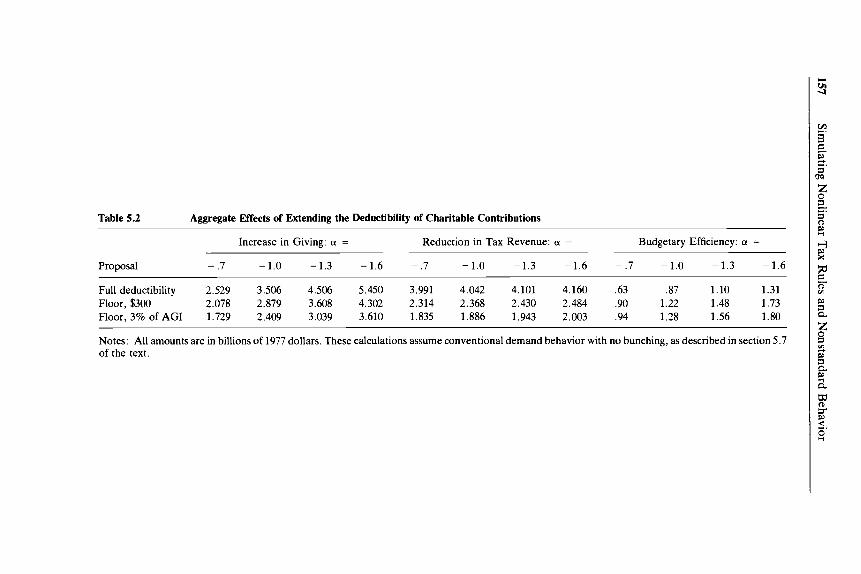
Table 5.2 summarizes the aggregate effects of alternative ways of extending the charitable deduction to nonitemizers. These estimates include not only the response of those who were nonitemizers in 1977 but also the changes in taxes and in giving among itemizers who would switch to nonitemizer status if the tax rule were changed.

Consider, for example, the effect of full deductibility with a price

24. See Clotfelter (1980) on the difference between the long-run and the short-run responses to changes in tax rates. The response to a permanent change in tax rules might, however, be more rapid than the response to transitory changes in tax rates.

25. Although these figures do not correspond exactly to published IRS numbers because we have used a sample of returns, the large size of the sample guarantees that errors are very small.

Table 1 Actual and Imputed Charitable Contributions

Number of Returns Mean Charitable Gift ( x 1,000

Nonitemizers: a = AGI Class Non- ( x 1,000) Itemizers itemizers Itemizers - .7 - 1.0 - 1.3 - 1.6

Less than $5,000 194 23,261 364 212 209 206 204 $5410 1,486 18,249 419 341 334 327 320 $1&$15 3,057 10,488 522 322 307 293 279 $15-$20 4,671 7,247 509 415 391 368 346 $2&$25 4,772 3,017 568 366 336 308 282 $25-$30 3,209 1,191 679 495 416 352 298 $30-$50 4,193 57 1 917 624 552 485 423 Over $50 1,336 83 4,029 600 550 497 447 All returns 22,916 64,108 819 307 295 283 273 Total ($ billion) . . . . . . 18,775 19,656 18,881 18,156 17,486

Note: Contributions of itemizers are the actual mean contributions of individuals who itemized their returns in 1977. Contributions of nonitemizers are imputed using the method described in section 5.3 of the text.

Table 5.2 Aggregate Effects of Extending the Deductibility of Charitable Contributions

Increase in Giving: a = Reduction in Tax Revenue: a = Budgetary Efficiency: a =

Proposal - .7 -1.0 -1.3 -1.6 -.7 -1.0 -1.3 -1.6 -.7 -1.0 -1.3 -1.6

Full deductibility 2.529 3.506 4.506 5.450 3.991 4.042 4.101 4.160 .63 .87 1.10 1.31 Floor, $300 2.078 2.879 3.608 4.302 2.314 2.368 2.430 2.484 .90 1.22 1.48 1.73 Floor, 3% of AGI 1.729 2.409 3.039 3.610 1.835 1.886 1.943 2.003 .94 1.28 1.56 1.80

Notes: All amounts are in billions of 1977 dollars. These calculations assume conventional demand behavior with no bunching, as described in section 5.7 of the text.


elasticity of - 1.0. The simulations imply that this would increase giving by $3.5 billion and would reduce tax revenue by $4.0 billion. For the nonitemizers alone, the price elasticity of 1 .O implies that the revenue loss would exactly equal the increase in giving. The excess of the revenue loss over the increased giving reflects the fact that previous itemizers who switch save substantially more in taxes than the increase, if any, in their giving. The “budgetary efficiency” estimate of 0.87 is the ratio of increased giving to reduced taxes implied by extending full deductibility to nonitemizers if the price elasticity is 1.

A more realistic price elasticity, of 1.3, implies a 29% higher level of increased giving but only 2% greater revenue loss. The budgetary efficiency value rises to 1.10, implying that charities receive an additional $1.10 for each extra dollar of revenue foregone by the Treasury.

Limiting the deduction of gifts by nonitemizers to the excess over $300 reduces both the revenue loss and the increased giving. With all these elasticities, the increase in giving is reduced by much less than the fall in revenue. With an elasticity of - 1.3, for example, the $300 floor reduces additional giving by $900 million (from $4.506 billion to $3.608 billion) but reduces the tax loss by nearly twice as much (from $4.101 billion to $2.430 billion, a decline of $1.7 billion).

A floor equal to 3% of AGI instead of a flat $300 has quite similar aggregate effects. With a price elasticity of - 1.3, giving falls $1.5 billion (from $4.506 billion to $3.039 billion) while the tax loss is reduced by more than $2.1 billion (from $4.101 to $1.943). Note that increasing the floor from $300 to 3% of AGI actually reduces giving by more than the saving in taxes; total giving falls an additional $569 million while the tax loss is cut by only $487 million. The primary reason for this is that the effect of the percent-of-AGI floor is concentrated more on those taxpayers with high marginal tax rates for whom the relative reductions are large.

Table 5.3 shows the changes in mean giving and tax liabilities in each AGI class and, for reference, the initial levels of giving and tax liabilities. These figures combine itemizers and nonitemizers. All of the calculations are based on a price elasticity of - 1.3.

Consider, for example, taxpayers in the $10,000 to $15,000 AGI class. Of the 13.5 million taxpayers in this group, 10.5 million were nonitemizers in 1977. Extending full deductibility of charitable gifts to all taxpayers would cause giving to increase by an average of $74 and taxes to fall by an average of $63. A $300 floor would reduce this increase in giving by $20 but would lower the fall in taxes by $30. Raising the floor from $300 to 3% of AGI would reduce giving by an average of $5 and would save an average of $4 in taxes.

Note that full deductibility has its maximum effect on the giving and taxes per return at the income levels between $15,000 and $20,000. Below

Table 5.3 Distribution of Changes in Mean Contributors and Tax Liabilities by Income Class

Increases in Giving and Reductions in Taxes

Number Initial Full Deducti- of Levels bility $300 Floor 3% AGI Floor

AGI Class Returns ( x 1,000) ( x 1,OOO) Giving Taxes Giving Taxes Giving Taxes Giving Taxes

Less than $5 23,455 208 11 5 5 5 3 4 4 $5-$10 19,735 334 437 61 54 46 32 52 35 $10-$15 13,545 344 1,206 74 63 54 33 49 29 $15-$20 11,918 423 2,078 93 84 80 52 65 38 $20-$25 7,789 467 3,026 61 59 49 32 29 18 $25-$30 4,399 591 4,274 61 57 50 34 26 16 $30-$50 4,763 865 6,879 50 50 46 35 24 15 Over $50 1,419 3,818 29,130 75 70 72 60 40 20 All returns 87,024 424 1,913 52 47 41 28 35 22 Total ($ billion) 87.024 36.931 166.456 4.506 4.101 3.608 2.430 3.039 1.943

Note: All calculations are based on a price elasticity of - 1.3 and refer to all taxpayers, including both current itemizers and nonitemizers.


$10,000 the relatively low marginal tax rates provide less incentive while above $20,000 the majority of taxpayers already itemize their deductions.

Imposition of a $300 floor would have virtually no effect on giving by taxpayers with AGIs over $25,000 since most such taxpayers would give more than $300 if deductibility were allowed. The absolute effect of the $300 floor on the mean level of giving is also greatest among taxpayers with incomes between $10,000 and $20,000. By contrast, a floor equal to 3% of AGI has a very substantial effect on the gifts and taxes of relatively high income taxpayers. A 3% floor virtually eliminates any tax saving for those with incomes over $25,000. Although total giving is lower with a 3% of AGI floor than with a $300 floor, giving by the large number of taxpayers with incomes under $10,000 is slightly higher.

Although table 5.2 suggests that a floor would be an “efficient” way of modifying the extension of the charitable deduction to all taxpayers (in the sense that it would save substantially more tax revenue than it would reduce charitable giving), table 5.3 indicates that a floor would also significantly change the distribution among income classes of both the increased giving and the reduced tax liability. Similarly, table 5.3 makes it clear that the choice between a $300 floor and a 3% of AGI floor involves not only aggregate efficiency considerations but also the income class distribution of the changes in giving and in tax liabilities. Of course, differences in the income class distribution of giving have significant effects on the types of charities that benefit.

5.5 Simulating Nonstandard Behavior

All of the calculations in section 5.4 were based on the conventional static utility maximization model of consumer demand for charitable giving. The more dynamic assumption that taxpayers respond to a floor by bunching contributions over time will be examined in the current section. The more radical departure from conventional utility maximization, the net altruism model of charitable giving, will also be considered.

5.5.1 Bunching Any floor on the charitable deduction would provide taxpayers with an

incentive to “bunch” their charitable contributions, giving a high level of contributions in some years and a low level in others. Because the existing law does not contain such a floor, we have no evidence about the likely extent of bunching. This section therefore presents simulation results for a rather broad range of two-year bunching assumptions. The restriction to a two-year cycle is significant and should be borne in mind in considering the results. All of the simulations refer to a price elasticity of - 1.3.

When a taxpayer responds to a floor by bunching his contributions, he reduces the amount of his giving that is not deductible and thereby


increases the tax saving associated with any level of giving. Moreover, to the extent that annual unbunched giving would be less than the floor while bunched giving exceeds the floor, the process of bunching also reduces the marginal price of giving and thus encourages increased giving. These two effects apply to both the “total bunching” and “partial bunching” models described in section 5.2.

Recall that, with the total bunching model, the probability that individual i will bunch is given by

(5.1) PROBi = 1 - (BCGli/CGli)’ ,

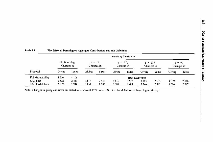
where CGli is the net cost to taxpayer i of giving the amount that he would choose to give in the presence of a floor if he does not bunch and BCGli is the net cost of giving that amount with bunching. Table 5.4 presents simulation results with four different values of the bunching sensitivity variable.

The striking feature of the results in this table is that bunching appears to have only a very modest effect on both tax revenue and giving. For example, a $300 floor with no bunching reduces giving by $898 million, from $4.506 billion to $3.608 billion. With the bunching described by the moderate sensitivity value of p = 2, the decline in giving is reduced from $898 million to $861 million. Even with the high sensitivity value of p = 10, giving is still reduced by $743 million. Indeed, even the limiting case in which everyone who can benefit from bunching does bunch still leaves the extra giving $427 million lower than without a floor.

The effect of bunching on tax revenue is limited in a similar way. Without bunching, the $300 floor reduces the revenue loss by $1.671 billion, from $4.101 billion to $2.430 billion. Even with the high sensitivity value of p = 10, the $1.671 billion revenue effect on the floor is reduced by only $175 million. This very small effect of bunching on the revenue loss reflects the distribution of gifts by nonitemizers, particularly the large number of relatively small gifts, for which the floor would eliminate all or nearly all deductibility. An individual who gave less than $150 a year without bunching would get no deduction even if she bunched completely. And a taxpayer who gave $400 every other year instead of $200 each year still would get a deduction for only one-fourth of her total giving.

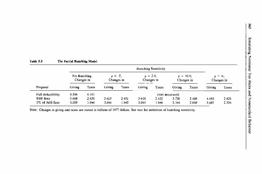
Table 5.5 presents results for the partial bunching model, in which all taxpayers who can benefit from bunching do bunch at least part of their gift. The results are similar to the probabilistic total bunching model of table 5.4 but indicate even smaller effects on giving and tax revenue.26

26. The figures for full and partial bunching with p = 30 would be exactly equal if there were no gifts of appreciated property. The small difference in our calculations reflects differences in the assumed realization of capital gains.

Table 5.4 The Effect of Bunching on Aggregate Contribution and Tax Liabilities

Bunching Sensitivity

No Bunching, p = . 5 , p = 2.0, p = 10.0, P = m, Changes in Changes in Changes in Changes in Changes in

Proposal Giving Taxes Giving Taxes Giving Taxes Giving Taxes Giving Taxes

Full deductibility 4.506 4.101 (NOT RELEVANT) $300 floor 3.608 2.430 3.617 2.442 3.645 2.447 3.763 2.605 4.079 2.818 3% of AGI floor 3.039 1.944 3.051 1.955 3.089 1.988 3.246 2.112 3.686 2.347

Note: Changes in giving and taxes are stated in billions of 1977 dollars. See text for definition of bunching sensitivity.

Table 5.5 The Partial Bunching Model

Bunching Sensitivity ~~~ ~

No Bunching, p = .5, p = 2.0, p = 10.0, P = w,

Changes in Changes in Changes in Changes in Changes in

Proposal Giving Taxes Giving Taxes Giving Taxes Giving Taxes Giving Taxes ~ ~~~

Full deductibility 4.506 4.101 (NOT RELEVANT) $300 floor 3.608 2.430 3.615 2.431 3.616 2.432 3.730 2.498 4.093 2.825 3% of AGI floor 3.039 1.944 3.044 1.945 3.045 1.946 3.164 2.008 3.697 2.354



Since there is no experience with floors on which to base empirical estimates of the taxpayers’ likely response, it is reassuring that the results of this section are not sensitive to a wide variation in assumptions about the possible extent of bunching. It should, however, be borne in mind that only two-year bunching was considered and that if taxpayers bunched over a longer period the effects would be more substantial.

5.5.2 Net Altruism The “net altruism” model of charitable giving described in section

5.2.3 implies that individuals choose the amount to contribute to charity to achieve a desired net cost to themselves. Individual differences in the desired net cost reflect differences in income and taste. Alternative tax rules affect charitable giving by altering the amount that individuals can contribute per dollar of net cost. Any loss in tax revenue is matched by an equal increase in charitable giving.

In the simple context of extending the charitable deduction without any floor, net altruism is equivalent to a price elasticity of - 1 for the nonitemizers themselves. However, net altruism implies that the taxpayers who switched from itemizing to using the standard deduction will add the resulting tax saving to their charitable gifts. Moreover, where giving causes a reduction in marginal tax rates, the net altruist contributes all of the inframarginal tax saving while traditional demand behavior implies that inframarginal saving has only a small income effect. The difference between the conventional demand model with unitary price elasticity and the net altruism model is shown in the first row of table 5.6.

The contrast between conventional demand and net altruism is much greater where there are floors. Table 5.6 shows that the conventional demand model with a unitary price elasticity implies that a $300 floor causes giving to fall by $600 million and increases tax revenue $1.7 billion. With net altruism, the reduced deductibility has a much greater effect on giving. Giving falls by $1.9 billion, and the tax revenue rises by an equal amount. The results are similar if the floor is stated as a percent of AGI.

If the net altruism model reflects reality, extending the deduction with a floor does not have greater budgetary efficiency than full deductibility. Introducing the floor in itself no longer increases tax revenue by more than it reduces giving. With net altruism, the principal reason for having a floor is to reduce the scale and cost of extending deductibility. The floor would of course also affect the income class distribution of the induced changes in giving and tax payments and therefore the mix of donees that benefit.

The choice between the net altruism model and the conventional demand model cannot be settled decisively with the available evidence. To the extent that the estimated price elasticity is significantly different from - 1, the data do support a conventional demand analysis. But it is

Table 5.6 The Effect of Net Altruism Behavior on Aggregate Contributions and Tax Liabilities

Conventional Demand with a = -1 Net Altruism

Changes in Changes in Budgetary Budgetary

Proposal Giving Taxes Efficiency Giving Taxes Efficiency

Full deductibility 3.506 4.042 367 3.871 3.951 .979 $300 floor 2.879 2.368 1.216 1.963 2.008 .978 3% of AGI floor 2.409 1.886 1.277 1.543 1.573 .980



quite possible that some individuals behave according to net altruism principles while the behavior of others is best described by a conventional demand analysis. If so, the observed price elasticity is a misleading guide to what would happen if deductibility with a floor were extended. The results would then be some mix between the net altruism behavior of table 5.6 and the conventional demand response with a price elasticity between - 1.3 and - 1.6.

5.6 Concluding Remarks

The primary purpose of the present paper is methodological: to examine how tax simulation could be extended to incorporate nonlinear budget constraints and nonstandard economic behavior. We have shown how econometric estimates derived under existing tax rules can be extended to deal with this wider range of simulations. On those issues for which existing evidence is not informative we have presented simulations that indicate the sensitivity of the conclusion to the unknown aspects of behavior.

The specific simulations indicate that the econometric evidence on charitable giving implies that extending the charitable deduction to nonitemizers would raise individual giving by about 12% of the existing total amount, or $4.5 billion at 1977 levels. The extension would reduce tax revenue by slightly less, about $4.1 billion. A floor of $300 or 3% of AGI would reduce the revenue loss by 30 to 40%, even if there were significant bunching. The effect of the floor on increased giving depends critically on whether taxpayers’ behavior is guided by conventional demand principles or by the net altruism rule. A reasonable conclusion is that a floor would reduce giving by less than the increased revenue but that the difference between them would not be very large.

In conclusion, it should perhaps be stressed that the appropriate tax treatment of charitable contributions depends on much more than the effects of alternative tax rules on the magnitude and distribution of contributions and taxes. Andrews (1972), for example, has argued that a correct definition of net income requires deducting charitable gifts while Surrey (1973) has argued the opposite. Feldstein (1980) has emphasized that a tax subsidy of individual giving may be preferable to government spending for the same purpose even when a dollar of tax revenue loss induces less than a dollar of additional giving, if individual giving is influenced by the level of government spending on the particular activity. Still others have emphasized the administrative and compliance problems associated with extending the deduction to low income taxpayers, who are rarely audited. All these considerations are important but lie beyond the scope of the current paper.


References

Andrews, W. D. 1972. Personal deductions in an ideal income tax. Harvard Law Review 86 (December): 309-85.

Boskin, M. J. , and M. Feldstein. 1977. Effects of the charitable deduction on contributions by low-income and middle-income households: Evidence from a national survey of philanthropy. Review of Economics and Statistics 59 (August) : 35 1-54.

Clotfelter, C. T. 1980. Tax incentives and charitable giving: Evidence from a panel of taxpayers. Journal of Public Economics 13: 31940.

Clotfelter, C. T., and C. E. Steuerle. 1979. The effect of the federal income tax on charitable giving. Mimeo, Duke University and Office of Tax Analysis, United States.

Dye, R. F. 1977. Personal charitable contributions: Tax effects and other motives. In Proceedings of the National Tax Association, pp. 311-18. Columbus Ohio: National Tax Association-Tax Institute of America.

Feldstein, M. 1975a. The income tax and charitable contributions. Part 1. Aggregate and distributional effects. National Tax Journal 28: 81-100.

. 1975b. The income tax and charitable contributions. Part 2. The impact on religious, educational, and other organizations. National Tax Journal 28: 209-26.

. 1980. A contribution to the theory of tax expenditures: The case of charitable giving. In H. Aaron and M. Boskin, eds., Essays in honor of Joseph Pechman. Washington: Brookings Institution.

Feldstein, M. and C. Clotfelter. 1976. Tax incentives and charitable contributions in the United States. Journal of Public Economics 5 :

Feldstein, M. and A. Taylor. 1976. The income tax and charitable con-

Hausman, J . A. 1979. Exact consumer’s surplus. Massachusetts Institute

Reece, W. S. 1979. Charitable contributions: New evidence on house-

Surrey, S. S. 1973. Pathways to tax reform. Cambridge: Harvard Uni-

1-26.

tributions. Econometricu 44: 1201-22.

of Technology. Mimeo.

hold behavior. American Economic Review 69: 142-51.

versity Press.

Comment Harvey Galper

My general overall evaluation of the Feldstein-Lindsey paper (hereafter F-L) is that it is an ideal illustration of how tax simulation work should

Harvey Galper at the time of this writing was director, Office of Tax Analysis, United States Treasury. He is currently a senior fellow at the Brookings Institution.


proceed methodologically. Modeling behavioral responses to tax changes is not an easy undertaking. The data base one has to deal with may be incomplete in several respects; the particular tax changes which one may want to simulate may not be easily translatable to price and income effects, which economists are accustomed to dealing with; and the empirical literature may not always provide guidance on which price and income elasticities to apply. Yet, as this paper demonstrates, through imaginative solutions simulation results can be provided on various effects of proposed changes in tax law.

I do, however, have some comments to make on this paper, starting with the review of the empirical literature. There has accumulated over the last five years a significant literature on the responsiveness of charitable contributions to the tax price, much of this literature resulting from efforts of one of the current authors. The tax price is defined essentially as 1 minus the marginal tax rate of the donor, although some modifications for appreciated property may also be required. From a review of the literature F-L conclude that the elasticity of giving with respect to the tax price is quite high-on the order of 1.3 in absolute terms-and that this same elasticity can be used to describe the tax behavior of nonitemizers. This is a very key assumption in the analysis in this paper, even though simulations with lower elasticities are also examined to some degree.

I find it quite difficult to accept as the general case an elasticity as high as 1.3 for nonitemizers. On a priori grounds, there are reasons why nonitemizers may be expected to exhibit less sensitivity to tax prices for charitable contributions. In fact, one reason why taxpayers may even take the standard deduction is that they are less sensitive to tax prices.

In the end, of course, the question is an empirical one. And while the literature has demonstrated clearly that individuals with higher marginal tax rates are highly sensitive to the price of giving, the case in my view has not been made for lower-income nonitemizers. In an excellent article that reviews this literature and provides evidence of their own empirical work, Clotfelter and Steuerle conclude that “estimates of the price elasticity tend to vary by income class and are sensitive to the specification of the regression model. The estimates from the most reasonable cross-sectional specifzcations range from - 0.4 to - 0.9 for low income taxpayers to - 1.7 to - 1.8 for high income taxpayers.”’

Other researchers have also found a significant relation between higher absolute elasticity and higher income.* It is true that various specifications

1. C. T. Clotfelter and C. E. Steuerle, “Charitable Contributions,” in H. J . Aaron and J. A . Pechman, eds., How Taxes Affect Economic Behavior (Washington: Brooking Institution, 1981), emphasis added.

2. See, for example, M. Feldstein, “The Income Tax and Charitable Contributions,’’ part 1, “Aggregate and Distributional Effects,” National TaxJournal, vol. 28 (March 1975); M. Feldstein and A. Taylor, “The Income Tax and Charitable Contributions,’’ Economer-


do cause the results to bounce around. But I would interpret the weight of evidence as indicating more modest price elasticities for lower-income taxpayers. Adding a possible lower tax consciousness for nonitemizers, I would conclude that an elasticity of about - 0.7 would be more charac- teristic of lower-income nonitemizers.

As an aside, it should be noted that the econometric problems with respect to estimating the response of behavior such as charitable giving to tax prices have not been fully resolved. To a degree, the problem of simultaneity between giving and tax price is handled by taking as the measure of tax price the first-dollar price, that is, the price if there were no charitable contributions made at all, rather than the last-dollar price, or the price from the last dollar of contributions made. Indeed, the empirical literature on this subject invoked by F-L in defending the - 1.3 elasticity assumption generally uses the first-dollar price or some variant of it. One obvious problem is that for the actual simulations in this paper, the price elasticity is assumed to be that appropriate for the last-dollar price rather than the first-dollar price. The question here is, Are there any reasons to expect elasticity with respect to the last-dollar price, assuming it can be accurately estimated, to be significantly different from that found from reviewing the literature on the first-dollar price?

Another much more general question is whether the decision to make a charitable contribution can be legitimately examined under the assumption that all other itemized deductions are given. In other words, itemization may be a much more complex simultaneous process than can be modeled by treating each deduction separately. There are obvious statistical problems in attempting to estimate several possible itemized deductions simultaneously all subject to a schedule of rising marginal tax rates. However, there are instances in this paper where implicitly or explicitly this simultaneity issue is raised. For example, some of the elasticity findings from the empirical literature reported in the paper are based on the assumption that itemizers will continue to itemize even if, in the absence of charitable giving, they find it advantageous to use the standard deduction. The implicit assumption must be that other deductions can be taken to offset the possible decline in contributions. If this is so, then itemized deductions are indeed interrelated and cannot be examined independently.

Also, the discussion of bunching by F-L implies that a legitimate response to a proposal that allows a deduction only for charitable contributions in excess of a floor amount is to concentrate deductions in particular years, that is, to try to exceed the floor in those years even if this is not possible in every year. However, why cannot this be done for all

rica vol. 44 (November 1976); E. M. Sunley, “Federal and State Tax Policies,” in D. W. Breneman and C . E. Finn, Jr. , eds., Public Policy and Private Higher Education (Washing- ton: Brookings Institution, 1978).

170 Martin FeldsteinJLawrence B. Lindsey

itemized deductions together in order to exceed the standard deduction in some years? That is, a taxpayer could conceivably alter the timing of payment of interest, taxes, and medical bills in addition to charitable contributions. If a taxpayer has such flexibility, there is again the possibility of an interdependence of deductions. Clotfelter especially has emphasized that the interaction between aparticulur itemized deduction and the decision to itemize can bias the estimates of elasticities in particular samples.

These comments are offered only in the spirit of encouraging additional work in this area. With our current state of knowledge, there is probably little more that can be done in the way of incorporating such effects into existing tax simulation models.

In the analysis of extending the contribution deduction to nonitemizers, I found very appealing the use of a utility function approach to analyze consumer choices under nonlinear budget constraints. However, I must confess to some disenchantment with the “net altruism” notion. According to this notion, individuals want to make a fixed net, that is, after-tax, contribution to charities regardless of the tax price. It is certainly true algebraically that such an approach is indistinguishable from an elasticity of - 1 in a traditional demand analysis. However, unlike a traditional demand analysis, the net altruism notion implies that the donor derives no utility whatsoever from the funds received, and dis- bursed, by the philanthropic organization-whether for health research, education, or the cultural enrichment of the community. Only the amount of individual sacrifice is of concern to the donor. Such altruism seems of a strange sort indeed.

The treatment of bunching is an intriguing way of dealing with an unobservable possibility-the concentration of gifts in particular years in response to allowing charitable deductions only in excess of a floor amount. In fact, this is illustrative of the ingenuity required to use and run simulation models in general. Very often, the particular tax proposals to be analyzed do not lend themselves to strictly linear price and income rules. The tax law abounds in floors, phaseout ranges, and complex interactions which not only make the calculation of the tax price itself very difficult but also cause taxpayers to engage in maximizing behavior that may involve intertemporal shifts of income or deductions. The approach must be the one that is followed here: allow a range of possible taxpayer responses and examine the sensitivity of the results.

Before simulations of the effects of allowing nonitemizers to deduct charitable contributions can be performed, it is necessary first to impute current charitable contributions to nonitemizers. I have some reserva-

3. C. T. Clotfelter, “Tax Incentives and Charitable Giving: Evidence from a Panel of Taxpayers,” Journal of Public Economics, vol. 13, no. 3 (June 1980).


tions about the imputation procedure used in the NBER model. One indication of my concern is that the total volume of giving by nonitemiz- e r s - o n the order of $18.5 billion-seems very high. Total contributions of itemizers and nonitemizers amounted to about $37 billion in 1977 under the F-L imputation procedures. This amount is about one-quarter higher than the most recent estimate for 1977 ($29.3 billion) set forth in Giving USA, a publication that reports on trends in American philanthr~py.~ This would result in a ratio of total giving to personal income of 2.4%, 20% greater than the previous peak of 2.0% , reached in 1970. Treasury imputations for 1977 of the giving of nonitemizers are $12.3 billion, about two-thirds of the F-L result. This yields a total contribution figure of $30 billion, quite close to the Giving USA estimate.

Since the NBER imputation procedure reflects the assumption that the only difference between nonitemizers and itemizers is that the two groups face different tax prices and incomes, this assumption itself may require reexamination. The imputation procedures in the Treasury model take a somewhat different approach. The Treasury model makes imputations for all itemized deductions simultaneously, subject to the constraint that the sum of all such imputed deductions cannot exceed the zero bracket amount (the standard deduction).

F-L recognizes that imputations cannot be so high as to cause taxpayers to itemize, and they try to control for this in their imputation procedures in two ways. First, nonitemizers are only compared with those itemizers who would continue to itemize even if they made no charitable contributions. That is, those who itemize only because of large charitable contributions are excluded from the reference group. Second, the model truncates imputed giving to reduce the possibility of excessively high imputations. These procedures, however, are not particularly contrain- ing. The first restriction eliminates just the greatest outliers among the itemizers, and the truncation procedure has even less effect. For example, a joint return with AGI of $50,000 is still allowed a maximum imputed gift of $1,700, almost twice the average giving of itemizers in the $30,000 to $50,000 income class. For lower-income taxpayers, the truncation is even less stringent. I would therefore encourage some experi- mentation with a simultaneous imputation procedure in which all itemizable expenses are imputed to nonitemizers but under the constraint that their sum cannot exceed the standard deduction. (One by-product of this approach is that other itemizable expenses can also be examined to determine their sensitivity to tax prices.)

A few comments on the simulations themselves may be in order. First, since, except for the net altruism variant, floors on deductible contribu-

4. American Association of Fund Raising Journal, Giving USA, 25th Annual Issue, New York, 1980, p. 11.


tions serve to reduce the revenue loss considerably without greatly affect- ing giving, a case could be made for adding a floor to current law- perhaps using the revenue gain for general rate cuts. If the simulations presented are reasonably accurate, the revenue gain is likely to be much greater than the cutback in giving. The results of such a simulation would be quite interesting.

Second, it is now possible to estimate not only the long-run effect of these changes in tax rules, as presented in the F-L paper, but also the short-run effects on a year-to-year basis by applying the work of C l~ t f e l t e r .~ Clotfelter finds considerable lags in adjusting to desired long- run behavior and estimates a six-year time period for 90% of the long-run solution to be realized. Furthermore, in the case of allowing nonitemizers to deduct charitable contributions, the lags may be somewhat longer since Clotfelter also finds that new itemizers display less sensitivity to price changes than former itemizers.

As a final comment, a point made by Kenneth Arrow in discussing the use of microeconomic simulation models for public policy analysis is worth emphasizing here. Arrow was critical of the excessive preoccupa- tion with budgetary costs in simulation models to the exclusion of the economist’s main concerns-equity and efficiency. In his words, “theoretically, the only justification for even considering budgetary costs as such is that they are financed by taxes which have their own distortion- ary ~ignificance.”~ This comment is applicable to the current paper as well. Even if the revenue loss is less than the increase in giving, the revenue loss still must be made up in some fashion. Why not make fuller use of the considerable effort and ingenuity that have gone into the development of this model by undertaking a more complete analysis of this issue? In particular, the utility functions developed to determine consumer choices are just the tool needed to satisfy Arrow’s concern.

It would be possible to examine alternative ways of raising the revenue that is lost by the proposals examined here to see who the gainers and losers are in a net sense and also to analyze whether overall social welfare has been improved. This would then provide the framework for an even more general approach in which the increase in tax rates required to finance these proposals affects other aspects of behavior such as the supply of savings and labor. With such an analysis, we will be able to break out of the mold of narrowly comparing the revenue loss and the giving gain as if an elasticity of - 1 really meant something.

5. Clotfelter, “Tax Incentives and Charitable Giving.” 6. K. J . Arrow, “Microdata Simulation: Current Status Problems, Prospects,” in R. H.

Haveman and K. Hollenbeck, eds., Microeconomic Simulation Models for Public Policy Analysis, vol. 2 (New York: Academic Press, 1980), p. 264.

Date post:	10-Mar-2018
Category:	Documents
Upload:	lelien
View:	225 times
Download:	1 times

Simulating Nonlinear Tax Rules and Nonstandard … Simulating Nonlinear Tax Rules and Nonstandard...

Documents