Simulating propagation of decoupled elastic waves using low-rankapproximate mixed-domain integral operators for anisotropic media

Jiubing Cheng1, Tariq Alkhalifah2, Zedong Wu2, Peng Zou3, and Chenlong Wang3

ABSTRACT

In elastic imaging, the extrapolated vector fields are de-coupled into pure wave modes, such that the imaging con-dition produces interpretable images. Conventionally, modedecoupling in anisotropic media is costly because the oper-ators involved are dependent on the velocity, and thus theyare not stationary. We have developed an efficient pseudo-spectral approach to directly extrapolate the decoupled elas-tic waves using low-rank approximate mixed-domainintegral operators on the basis of the elastic displacementwave equation. We have applied k-space adjustment tothe pseudospectral solution to allow for a relatively largeextrapolation time step. The low-rank approximation was,thus, applied to the spectral operators that simultaneouslyextrapolate and decompose the elastic wavefields. Syntheticexamples on transversely isotropic and orthorhombic mod-els showed that our approach has the potential to efficientlyand accurately simulate the propagations of the decoupledquasi-P and quasi-S modes as well as the total wavefieldsfor elastic wave modeling, imaging, and inversion.

INTRODUCTION

Multicomponent seismic data are increasingly acquired on landand at the ocean bottom in an attempt to better understand the geo-logic structure and characterize oil and gas reservoirs. Seismic mod-eling, reverse time migration (RTM), and full-waveform inversion(FWI) in areas with complex geology all require high-accuracynumerical algorithms for time extrapolation of waves. Because seis-mic waves propagate through the earth as a superposition of P- andS-wave modes, an elastic wave equation is usually more accuratefor wavefield extrapolation than an acoustic wave equation. Wave

mode decoupling can not only help elastic imaging to producephysically interpretable images, which characterize reflectivitiesof various reflection types (Wapenaar et al., 1987; Dellinger andEtgen, 1990; Yan and Sava, 2008), but it can also provide moreopportunity to mitigate the parameter trade-offs in elastic waveforminversion (Wang and Cheng, 2015).For isotropic media, far-field P and S waves can be separated by

taking the divergence and curl in the extrapolated elastic wavefields(Aki and Richards, 1980; Sun and McMechan, 2001). Alternatively,Ma and Zhu (2003) and Zhang et al. (2007) extrapolate vector P andS modes separately in an elastic wavefield by decomposing thewave equation into P- and S-wave components. In the meantime,decoupling of the wave modes yields familiar scalar wave equationsfor the P and S modes (Aki and Richards, 1980). In anisotropicmedia, one cannot derive explicit single-mode time-space-domaindifferential wave equations so simply. Generally, P and S modes donot respectively polarize parallel and perpendicular to the wave vec-tors, and thus they are called quasi-P (qP) and quasi-S (qS) waves.They cannot be fully decoupled with divergence and curl operations(Dellinger and Etgen, 1990).Anisotropic wave propagation can be formally decoupled in the

wavenumber domain to yield single-mode pseudodifferential equa-tions (Liu et al., 2009). Unfortunately, these equations in the time-space domain cannot be solved with traditional numerical schemesunless further approximation to the dispersion relation or phasevelocity is applied (Etgen and Brandsberg-Dahl, 2009; Chu et al.,2011; Fowler and King, 2011; Zhan et al., 2012; Song and Alkha-lifah, 2013; Du et al., 2014; Wu and Alkhalifah, 2014). To avoidsolving the pseudodifferential equation, Xu and Zhou (2014) pro-pose a nonlinear wave equation for pseudoacoustic qP-wavewith anauxiliary scalar operator depending on the material parameters andthe phase direction of the propagation at each spatial location. Allthese efforts are restricted to pure-mode scalar waves and do nothonor the elastic effects such as mode conversion. Cheng and Kang(2014) and Kang and Cheng (2012) propose approaches to propa-

Manuscript received by the Editor 18 March 2015; revised manuscript received 21 October 2015; published online 15 March 2016.1Tongji University, State Key Laboratory of Marine Geology, Shanghai, China. E-mail: cjb1206@tongji.edu.cn.2King Abdullah University of Science and Technology, Thuwal, Saudi Arabia. E-mail: tariq.alkhalifah@kaust.edu.sa; zedong.wu@kaust.edu.sa.3Tongji University, Shanghai, China. E-mail: 1533006@tongji.edu.cn; skoltyz.10000@163.com.© 2016 Society of Exploration Geophysicists. All rights reserved.

T63

GEOPHYSICS, VOL. 81, NO. 2 (MARCH-APRIL 2016); P. T63–T77, 12 FIGS.10.1190/GEO2015-0184.1

Dow

nloa

ded

05/0

3/16

to 1

09.1

71.1

37.2

10. R

edis

trib

utio

n su

bjec

t to

SEG

lice

nse

or c

opyr

ight

; see

Ter

ms

of U

se a

t http

://lib

rary

.seg

.org

/

gate the partially decoupled wave modes using the so-called pseudopure-mode wave equations, and then they obtain completely de-coupled qP or qS waves by correcting the polarization deviationof the pseudo pure-mode wavefields. Their approaches honor thekinematics of all wave modes but may distort the reflection/trans-mission coefficients if high contrasts exist in the velocity fields.Alternatively, many have developed approaches to decouple the

qP- and qS-wave modes from the extrapolated elastic wavefields.Dellinger and Etgen (1990) generalize the divergence and curloperations to anisotropic media by constructing separators as polari-zation projection in the wavenumber domain. To tackle hetero-geneity, these mode separators are rewritten by Yan and Sava(2009) as nonstationary spatial filters determined by the localpolarization directions. Zhang and McMechan (2010) propose awavefield decomposition method to separate elastic wavefields intovector qP and qS wavefields for vertically transverse isotropic (VTI)media. Accordingly, Cheng and Fomel (2014) propose fast mixed-domain algorithms for mode separation and vector decompositionin heterogeneous anisotropic media by applying low-rank approxi-mation to the involved Fourier integral operators (FIOs) of the gen-eral form.The motivation of this study is to develop an efficient approach to

propagate and decouple the elastic waves for general anisotropicmedia. The primary strategy is to merge the numerical solutionsfor time extrapolation and vector decomposition into a unified Fou-rier integral framework and speed up the solutions using the low-rank approximation. This paper is organized as follows: We firstdemonstrate a pseudospectral solution to extrapolate the elastic dis-placement wavefields in the time domain. Then, we propose tomerge the spectral operations for time extrapolation into the integralframework for vector decomposition of the wave modes. Applyinglow-rank approximations to the involved mixed-domain matrices,we obtain an efficient algorithm for simultaneous propagatingand decoupling the elastic wavefields. We demonstrate the validityof the proposed method using 2D and 3D synthetic examples on thetransversely isotropic (TI) and orthorhombic models with increas-ing complexity.

PROPAGATING COUPLED ELASTICWAVEFIELDS

Following Carcione (2007), we denote the spatial variablesx, y, and z of a right-hand Cartesian system by the indicesi; j; : : : ¼ 1;2, and 3, respectively, the position vector by x, a partialderivative with respect to a variable xi with ∂i, and the first and sec-ond time derivatives with ∂t and ∂tt, respectively. Matrix transpo-sition is denoted by the superscript T. We also denote

ffiffiffiffiffiffi−1

pby i, the

scalar and matrix products by the symbol “·”, and the dyadic prod-uct by the symbol “⊗”. The Einstein convention of repeated indicesis assumed unless otherwise specified.

Pseudospectral solution of the elastic wave equation

Wave propagation in general anisotropic elastic media is gov-erned by the linearized momentum balance law and a linearconstitutive relation between the stress and strain tensors. Thesegoverning equations can be combined to write the displacement for-malism as follows:

ρ∂2ttu ¼ ∇ · ½C · ð∇T · uÞ� þ f; (1)

where u ¼ ðux; uy; uzÞT represents the vector wavefields, f is thebody force vector per unit volume, C is the 6 × 6 elasticity matrixrepresenting the stiffness tensor with the Voigt’s menu, and the spa-tial differential operator ∇ has the following matrix representation:

∇ ¼0@ ∂x 0 0 0 ∂z ∂y

0 ∂y 0 ∂z 0 ∂x0 0 ∂z ∂y ∂x 0

1A: (2)

The pseudospectral method calculates the spatial derivatives us-ing the fast Fourier transform (FFT), while approximating the tem-poral derivative with a finite difference (FD). Neglecting the sourceterm, equation 1 is rewritten in the spatial Fourier domain for ahomogeneous medium as follows:

∂2ttuþ Γu ¼ 0; (3)

where u is the wavefields in the wavenumber domain, k ¼ðkx; ky; kzÞ is the wavenumber vector, and Γ ¼ 1∕ρL · C · LT rep-resents the 3 × 3 density normalized Christoffel matrix (as shown inAppendix A) with the wavenumber-domain counterpart of the spacedifferential operator (removing the imaginary unit i) satisfies thefollowing equation:

L ¼0@ kx 0 0 0 kz ky

0 ky 0 kz 0 kx0 0 kz ky kx 0

1A: (4)

To calculate the second-order temporal derivatives, we use thestandard leapfrog scheme, i.e.,

∂2ttuðnÞi ¼ uðnþ1Þ

i − 2uðnÞi þ uðn−1Þi

Δt2; (5)

where Δt ¼ tnþ1 − tn is the time step. For constant-density homo-geneous media, applying the two-step time-marching scheme leadsto the following pseudospectral formula:

∂2ttuðnÞ ¼ ΨuðnÞ; (6)

with the spectral operator defined with the following kernel:

Ψ :¼ ð2πÞ−3ZZ

ΓðkÞeik·ðx−yÞdydk: (7)

Phase terms in the integral operator can be absorbed into forwardand inverse Fourier transforms. This implies that the wavefields arefirst transformed into the wavenumber domain using forward FFTs,multiplied with the corresponding components of the Christoffelmatrix, and finally transformed back into the space domain usinginverse FFTs. For locally smooth media, we use a spatially varyingChristoffel matrix to tackle the heterogeneity; i.e.,

Ψ :¼ ð2πÞ−3ZZ

Γðx; kÞeik·ðx−yÞdydk: (8)

The extended formation of this pseudospectral elastic wavepropagator is shown in Appendix B. Spectral methods are charac-terized by the use of Fourier basis functions to describe the fieldvariables and have an advantage over FD schemes in that the mesh

T64 Cheng et al.

Dow

nloa

ded

05/0

3/16

to 1

09.1

71.1

37.2

10. R

edis

trib

utio

n su

bjec

t to

SEG

lice

nse

or c

opyr

ight

; see

Ter

ms

of U

se a

t http

://lib

rary

.seg

.org

/

requirements are more relaxed (Kosloff et al., 1989; Liu andLi, 2000).

Adjustment to the pseudospectral solution

In general, the two-step time-marching pseudospectral solution islimited to a small time step because larger time steps lead to numeri-cal dispersion and stability issues. At higher computational costs,high-order FD (Dablain, 1986) can be applied to address this diffi-culty. As an alternative to second-order temporal differencing, atime integration technique based on rapid expansion method canprovide higher accuracy with less computational efforts (Kosloffet al., 1989). As Du et al. (2014) demonstrate, one-step time-march-ing schemes (Zhang and Zhang, 2009; Sun and Fomel, 2013), es-pecially using optimized polynomial expansion, usually give moreaccurate approximations to heterogeneous extrapolators for largertime steps. In this section, we discuss a strategy to extend the timestep for the previous two-step time-marching pseudospectralscheme according to the eigenvalue decomposition of the Christof-fel matrix.Because the Christoffel matrix is symmetric positive definite, it

has a unique eigen decomposition of the following form:

Γ ¼X3i¼1

λ2i ai ⊗ ai; (9)

where λ2i are the eigenvalues and ai are the eigenvectors of Γ withai · aj ¼ δij. The three eigenvalues correspond to phase velocitiesof the three-wave modes with λi ¼ vik (in which k ¼ jkj and virepresents the phase velocity) representing the circular frequency,and the corresponding eigenvector ai ¼ ðaix; aiy; aizÞ repre-sents the normalized polarization vector for the given mode. An al-ternative form of the above decomposition yields the followingequation:

Γ ¼ QΛQT; (10)

with

Λ ¼0@ λ21 0 0

0 λ22 0

0 0 λ23

1A; (11)

Q ¼0@ a1x a2x a3x

a1y a2y a3ya1z a2z a3z

1A: (12)

Note that Q is an orthogonal matrix; i.e., Q−1 ¼ QT .The eigenvalues represent the frequencies and satisfy the condi-

tion that is given by the following equation:

λi ¼ vik ≤ 2πfmax; (13)

where fmax is the maximum frequency of the source. Therefore, wesuggest to filter out the high-wavenumber components in the wave-fields beyond 2πfmax∕vmin (vmin is the minimum phase velocity inthe computational model) caused by the numerical errors to enhancenumerical stability.

According to above eigendecomposition, we apply the k-spaceadjustment to our pseudospectral scheme by modifying the eigen-values of the Christoffel matrix for the anisotropic elastic waveequation (see Appendix C), i.e.,

Λ¼0@λ21sinc

2ðλ1Δt∕2Þ 0 0

0 λ22sinc2ðλ2Δt∕2Þ 0

0 0 λ23sinc2ðλ3Δt∕2Þ

1A:

(14)

Thus, this adjustment inserts a modified Christoffel matrix, i.e.,Γ ¼ QΛQT , into the original pseudospectral formula on the basis ofequations 6 and 8. Note that the k-space adjustment to the pseudo-spectral solution has been widely used in acoustic and ultrasound(Bojarski, 1982; Tabei et al., 2002) and elastic isotropic wavefieldsimulation (Liu, 1995; Firouzi et al., 2012).

PROPAGATING DECOUPLED ELASTICWAVEFIELDS

The above pseudospectral operators propagate the elastic wave-fields as a superposition of qP- and qS-wave modes. To obtain

a)

b)

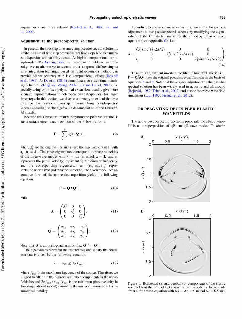
Figure 1. Horizontal (a) and vertical (b) components of the elasticwavefields at the time of 0.3 s synthesized by solving the second-order elastic wave equation withΔx ¼ Δz ¼ 5 m andΔt ¼ 0.5 ms.

Propagating anisotropic elastic waves T65

Dow

nloa

ded

05/0

3/16

to 1

09.1

71.1

37.2

10. R

edis

trib

utio

n su

bjec

t to

SEG

lice

nse

or c

opyr

ight

; see

Ter

ms

of U

se a

t http

://lib

rary

.seg

.org

/

physically interpretable results for seismic imaging and waveforminversion, wave mode decoupling is required during wavefieldextrapolation. The key concept of mode decoupling is based onpolarization. In a general anisotropic medium, the qP and qS modesdo not polarize parallel and perpendicular to the wave vectors.Moreover, unlike the well-behaved qP mode, the two qS modesdo not consistently polarize as a function of the propagation direc-tion (or wavenumber) and thus cannot be designated as SV and SHwaves, except in isotropic and TI media (Winterstein, 1990; Cram-pin, 1991). Even for a TI medium, it is a challenge to find the rightsolution of the shear singularity problem and obtain two completelyseparated S-modes with correct amplitudes (Yan and Sava, 2011;Cheng and Fomel, 2014). Therefore, we restrict to extrapolatethe decoupled qP- and qS-wave modes in this paper.

Vector decomposition of the elastic wave modes

According to Zhang and McMechan (2010), one can decomposeqP and qS modes in the elastic wavefields for a homogeneous aniso-tropic medium using the following equation:

uðmÞi ðkÞ ¼ DðmÞ

ij ðkÞ ~ujðkÞ; (15)

where m ¼ fqP; qSg, i; j ¼ fx; y; zg, and the decomposition oper-ators satisfy

DðqPÞxx ðkÞ ¼ a2xðkÞ;

DðqPÞyy ðkÞ ¼ a2yðkÞ;

DðqPÞzz ðkÞ ¼ a2zðkÞ;

DðqPÞxy ðkÞ ¼ axðkÞayðkÞ;

DðqPÞxz ðkÞ ¼ axðkÞazðkÞ;

DðqPÞyz ðkÞ ¼ ayðkÞazðkÞ; (16)

and

DðqSÞxx ðkÞ ¼ a2yðkÞ þ a2zðkÞ; DðqSÞ

yy ðkÞ ¼ a2xðkÞ þ a2zðkÞ;DðqSÞ

zz ðkÞ ¼ a2xðkÞ þ a2yðkÞ; DðqSÞxy ðkÞ ¼ −axðkÞayðkÞ;

DðqSÞxz ðkÞ ¼ −axðkÞazðkÞ; DðqSÞ

yz ðkÞ ¼ −ayðkÞazðkÞ;(17)

where axðkÞ, ayðkÞ, and azðkÞ respectively represent the x-, y-, andz-components of the normalized polarization vector of the qP-wave.As demonstrated by Cheng and Fomel (2014), one can decom-

pose the wave modes in a heterogeneous anisotropic medium usingthe following mixed-domain integral operations:

uðmÞx ðxÞ ¼

ZeikxDðmÞ

xx ðx; kÞ ~uxðkÞdk

þZ

eikxDðmÞxy ðx; kÞ ~uyðkÞdk

þZ

eikxDðmÞxz ðx; kÞ ~uzðkÞdk;

uðmÞy ðxÞ ¼

ZeikxDðmÞ

xy ðx; kÞ ~uxðkÞdk

þZ

eikxDðmÞyy ðx; kÞ ~uyðkÞdk

þZ

eikxDðmÞyz ðx; kÞ ~uzðkÞdk;

uðmÞz ðxÞ ¼

ZeikxDðmÞ

xz ðx; kÞ ~uxðkÞdk

þZ

eikxDðmÞyz ðx; kÞ ~uyðkÞdk

þZ

eikxDðmÞzz ðx; kÞ ~uzðkÞdk: (18)

a)

b)

c)

Figure 2. Vertical slices through the vertical components of the syn-thetic elastic wavefields at x ¼ 0.75 km: (a) 10th-order FD, (b) low-rank pseudospectral, and (c) low-rank pseudospectral using thek-space adjustment.

T66 Cheng et al.

Dow

nloa

ded

05/0

3/16

to 1

09.1

71.1

37.2

10. R

edis

trib

utio

n su

bjec

t to

SEG

lice

nse

or c

opyr

ight

; see

Ter

ms

of U

se a

t http

://lib

rary

.seg

.org

/

Extrapolating the decoupled elastic waves

For heterogeneous anisotropic media, the wavefield propagator(equation 6) and the vector decomposition operators (equation 18)are both in the general form of FIOs. Naturally, we merge them to

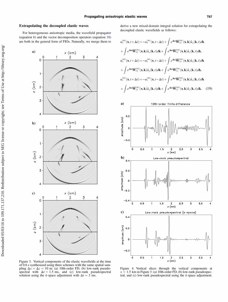
derive a new mixed-domain integral solution for extrapolating thedecoupled elastic wavefields as follows:

uðmÞx ðx;tþΔtÞ¼−uðmÞ

x ðx;t−ΔtÞþZ

eikxWðmÞxx ðx;kÞ ~uxðk;tÞdk

þZ

eikxWðmÞxy ðx;kÞ ~uyðk;tÞdkþ

ZeikxWðmÞ

xz ðx;kÞ ~uzðk;tÞdk;

uðmÞy ðx;tþΔtÞ¼−uðmÞ

y ðx;t−ΔtÞþZ

eikxWðmÞyx ðx;kÞ ~uxðk;tÞdk

þZ

eikxWðmÞyy ðx;kÞ ~uyðk;tÞdkþ

ZeikxWðmÞ

yz ðx;kÞ ~uzðk;tÞdk;

uðmÞz ðx;tþΔtÞ¼−uðmÞ

z ðx;t−ΔtÞþZ

eikxWðmÞzx ðx;kÞ ~uxðk;tÞdk

þZ

eikxWðmÞzy ðx;kÞ ~uyðk;tÞdkþ

ZeikxWðmÞ

zz ðx;kÞ ~uzðk;tÞdk; (19)

a)

b)

c)

Figure 3. Vertical components of the elastic wavefields at the timeof 0.6 s synthesized using three schemes with the same spatial sam-pling Δx ¼ Δz ¼ 10 m: (a) 10th-order FD, (b) low-rank pseudo-spectral with Δt ¼ 1.5 ms, and (c) low-rank pseudospectralsolution using the k-space adjustment with Δt ¼ 3 ms.

a)

b)

c)

Figure 4. Vertical slices through the vertical components atx ¼ 1.5 km in Figure 3: (a) 10th-order FD, (b) low-rank pseudospec-tral, and (c) low-rank pseudospectral using the k-space adjustment.

Propagating anisotropic elastic waves T67

Dow

nloa

ded

05/0

3/16

to 1

09.1

71.1

37.2

10. R

edis

trib

utio

n su

bjec

t to

SEG

lice

nse

or c

opyr

ight

; see

Ter

ms

of U

se a

t http

://lib

rary

.seg

.org

/

with the propagation matrices for the decoupled wave modes givenas

WðmÞij ðx; kÞ ¼ DðmÞ

ki ðx; kÞWkjðx; kÞ; (20)

where Wkjðx; kÞ is defined by the spatially varying Christoffel ma-trix and the length of time step, namely,

Wkkðx; kÞ ¼ 2 − Δt2Γkkðx; kÞ;Wkjðx; kÞ ¼ −Δt2Γkjðx; kÞ: (21)

The extended formulation of equation 20 is given in Appendix B.Note that symmetry properties exist: DðmÞ

ki ¼ DðmÞik and Wkj ¼ Wjk,

and the modified Christoffel matrix will be used if the k-space ad-justment is applied for the pseudospectral solutions.

To derive the time extrapolation of the decomposed wavefieldsusing equation 19, we must update the total elastic wavefields bysuperposing qP- and qS-waves at each time step using thefollowing equation:

uxðxÞ ¼ uðqPÞx ðxÞ þ uðqSÞx ðxÞ;uyðxÞ ¼ uðqPÞy ðxÞ þ uðqSÞy ðxÞ;uzðxÞ ¼ uðqPÞz ðxÞ þ uðqSÞz ðxÞ: (22)

Thus, equations 19–22 compose the spectral-like operators to si-multaneously extrapolate and decouple the elastic wavefields for3D anisotropic media. The computation complexity of the straight-

a) b)

c) d)

e) f)

Figure 5. Elastic wavefields at the time of 0.6 ssynthesized by using low-rank pseudospectral sol-ution of the displacement wave equation followedwith low-rank vector decomposition: (a) x- and(b) z-components of the displacement wavefields,(c) x- and (d) z-components of the qP wavefields,and (e) x- and (f) z-components of the qSV wave-fields.

T68 Cheng et al.

Dow

nloa

ded

05/0

3/16

to 1

09.1

71.1

37.2

10. R

edis

trib

utio

n su

bjec

t to

SEG

lice

nse

or c

opyr

ight

; see

Ter

ms

of U

se a

t http

://lib

rary

.seg

.org

/

forward implementation of the integral operators in equations 8 and19 is OðN2

xÞ, which is prohibitively expensive when the size ofmodel Nx is large.To tackle strong heterogeneity due to fast varying stiffness

coefficients, we suggest splitting the displacement equation intothe displacement-stress equation and then solving it using the stag-gered-grid pseudospectral scheme (Ozdenvar and McMechan,1996; Carcione, 1999; Bale, 2003). Note that when using stag-gered grids, the operators to extrapolate the decoupled wave modesmust be modified to account for the shifts in medium propertiesand fields variables. We will investigate this issue in futurework.

FAST ALGORITHM USING LOW-RANKDECOMPOSITION

As proposed by Cheng and Fomel (2014), low-rank decomposi-tion of the mixed-domain matrix dðx; kÞ in equation 18 yields a veryefficient algorithm for mode decoupling in heterogeneous aniso-tropic media. We find that the same strategy works for numericalimplementations of above pseudospectral operators for elastic wavepropagation.For example, the mixed-domain matrix, i.e., Wðx; kÞ or Wðx; kÞ

in the FIOs, can be approximated by the following separated rep-resentation (Fomel et al., 2013):

a) b)

c) d)

e) f)

Figure 6. Elastic wavefields at the time of 0.6 ssynthesized by using low-rank pseudospectral op-erators for extrapolating and decomposing theelastic waves simultaneously: (a) x- and (b) z-com-ponents of the qP-wave displacement wavefields,(c) x- and (d) z-components of the qSV-wave dis-placement wavefields, and (e) x- and (f) z-compo-nents of the total elastic wavefields.

Propagating anisotropic elastic waves T69

Dow

nloa

ded

05/0

3/16

to 1

09.1

71.1

37.2

10. R

edis

trib

utio

n su

bjec

t to

SEG

lice

nse

or c

opyr

ight

; see

Ter

ms

of U

se a

t http

://lib

rary

.seg

.org

/

Wðx; kÞ ≈PMm¼1

PNn¼1 Bðx; kmÞAmnCðxn; kÞ; (23)

where Bðx; kmÞ is a mixed-domain matrix with reduced wavenum-ber dimension M, Cðxn; kÞ is a mixed-domain matrix with reducedspatial dimension N, and Amn is an M × N matrix with N and Mrepresenting the rank of this decomposition. Physically, a separablelow-rank approximation amounts to selecting a set of N (N ≪ Nx)representative spatial locations and M (M ≪ Nx) representativewavenumbers. Construction of the separated representation followsthe method of Engquist and Ying (2009). The ranks M and N aredependent on the complexities (heterogeneity and anisotropy) ofthe medium and the estimate of the approximation accuracy tothe mixed-domain matrices (in the numerical examples, we aimfor the relative single-precision accuracy of 10−6). More explana-tions on low-rank decomposition are available in Fomel et al. (2013)and Cheng and Fomel (2014). As we observe, the ranks are gen-erally very small for our applications. For homogeneous media,the ranks naturally reduce to one. If there is heterogeneity, the ranksincrease to two for isotropic media but exceed two for anisotropicmedia. The k-space adjustment may slightly increase the ranks forthe heterogeneous media.Thus, the above low-rank approximation speeds up computation

of the FIOs as follows:ZeikxWðx;kÞ ~ujðkÞdk

≈XMm¼1

Bðx;kmÞ XN

n¼1

Amn

�ZeikxCðxn;kÞ ~ujðkÞdk

�!:(24)

a)

b)

c)

d)

e)

f)

g)

h)

i)

Figure 7. Synthesized decomposed and total elas-tic wavefields for a orthorhombic model with aVTI overburden: qP (top), qS (mid), and total (bot-tom) elastic displacement fields (left, x-compo-nent; mid, y-component; and right, z-component).

a)

b)

c)

Figure 8. The SEG/Hess VTI model with parameters of (a) verticalP-wave velocity, Thomsen coefficients (b) ϵ, and (c) δ.

T70 Cheng et al.

Dow

nloa

ded

05/0

3/16

to 1

09.1

71.1

37.2

10. R

edis

trib

utio

n su

bjec

t to

SEG

lice

nse

or c

opyr

ight

; see

Ter

ms

of U

se a

t http

://lib

rary

.seg

.org

/

Evaluation of the last formula is effectively equivalent to apply-ing N inverse FFTs each time step. Accordingly, the computationcomplexity reduces toOðNNx log NxÞ. In multiple-core implemen-tations, the matrix operations in equation 24 are easy to parallelize.

EXAMPLES

We will first demonstrate the proposed approach on two-layer TIand orthorhombic models, and then on the complex SEG Hess VTIand BP 2007 TTI models, respectively.

2D two-layer VTI/TTI model

The first example is on a 2D two-layer model, in which the firstlayer is a VTI medium with VP0 ¼ 2500 m∕s, VS0 ¼ 1200 m∕s,ϵ ¼ 0.2, and δ ¼ −0.2, and the second layer is a tilted TI

(TTI) medium with VP0 ¼ 3600 m∕s, VS0 ¼ 1800 m∕s, ϵ ¼ 0.2,δ ¼ 0.1, and θ ¼ 30°. A point source is placed at the center of thismodel. First, we compare the synthetic elastic wavefields by solvingthe elastic displacement wave equation using the 10th-order explicitFD and low-rank pseudospectral schemes (with or without thek-space adjustment), respectively. Figure 1 shows the wavefieldsnapshots at the time of 0.3 s using the spatial sampling Δx ¼ Δz ¼5 m and time step Δt ¼ 0.5 ms. Only the low-rank pseudospectralsolutions with the k-space adjustment are displayed because thethree schemes produce very similar results. The vertical slicesthrough the z-components of the elastic wavefields show fewdifferences among them (Figure 2). For the low-rank pseudospectralscheme, the ranks are all two for the decomposition of the mixed-domain matricesWxx,Wzz, andWxz in equation 21, and the k-spaceadjustment does not change the ranks. It takes CPU times of 0.20,0.23, and 0.23 s for them to finish the wavefield extrapolation of one

a) b)

c) d)

e) f)

Figure 9. Synthesized decoupled and total dis-placement fields using the low-rank pseudospectralsolution with the k-space adjustment that simulta-neously extrapolate and decouple qP and qSVwavefields in SEG/Hess VTI model: (a) x- and(b) z-components of qP-wavefields, (c) x- and(d) z-components of qSV wavefields, and (e) x-and (f) z-components of the total displacementfields.

Propagating anisotropic elastic waves T71

Dow

nloa

ded

05/0

3/16

to 1

09.1

71.1

37.2

10. R

edis

trib

utio

n su

bjec

t to

SEG

lice

nse

or c

opyr

ight

; see

Ter

ms

of U

se a

t http

://lib

rary

.seg

.org

/

time step. An additional 4.3 and 8.2 s have been used to finish thelow-rank decomposition of the involved mixed-domain matrices be-fore wavefield extrapolation. We observe the FD scheme is unstableif the time step is increased to 1.0 ms and the low-rank pseudospec-tral scheme is unstable if the time step is increased to 2.0 ms (withunchanged spatial sampling). However, the low-rank pseudospec-tral solution using the k-space adjustment produces acceptable re-sults even the time step is increased to 3.0 ms and the maximumtime exceeds 3 s. Figures 3 and 4 compare the wavefield snapshotsand the vertical slices at the time of 0.6 s using the three schemeswith the increased spatial sampling (namely, Δx ¼ Δz ¼ 10 m).The FD scheme tends to exhibit dispersion artifacts with the chosenmodel size and extrapolation step, whereas the low-rank pseudo-spectral scheme exhibits acceptable accuracy. The k-space adjust-ment permits larger time steps without reducing accuracy orintroducing instability. For this example, it has produced the best

results with less numerical dispersion. Thanks to the larger spatialand temporal sampling, the same CPU time is used for each schemeas in Figure 1. In addition, only the ranks for the low-rank decom-position of the matrix w12 reduce to one when we change the tiltangle of the second layer to zero.Second, we compare two approaches to get the decoupled elastic

wavefields during time extrapolation. The first approach uses thelow-rank pseudospectral algorithm to synthesize the elastic wave-fields and then applies the low-rank vector decomposition algorithm(Cheng and Fomel, 2014) to get the vector qP and qSV wavefields(Figure 5). The second extrapolates the decoupled qP- and qSV-wavefields using the proposed low-rank mixed-domain integral op-erations (Figure 6). Extrapolation steps of Δx ¼ Δz ¼ 10 m andΔt ¼ 1.0 ms are used in this example. The ranks are still twofor the involved low-rank decomposition of the propagation matri-ces defined in equation 20. The two approaches produce compa-

a)

d)

b)

c)

e) f)

Figure 10. Elastic wavefield extrapolation using10th-order FD scheme and low-rank vector decom-position in SEG/Hess VTI model: (a) x- and (b) z-components of the synthetic elastic displacementwavefields at 1.1 s, (c) x- and (d) z-componentsof vector qP wavefields, and (e) x- and (f) z-com-ponents of vector qSV wavefields.

T72 Cheng et al.

Dow

nloa

ded

05/0

3/16

to 1

09.1

71.1

37.2

10. R

edis

trib

utio

n su

bjec

t to

SEG

lice

nse

or c

opyr

ight

; see

Ter

ms

of U

se a

t http

://lib

rary

.seg

.org

/

rable elastic wavefields, in which we can observe all transmitted andreflected waves including mode conversions. For one step of thetime extrapolation, it takes the CPU time of 0.6 ms for the first ap-proach and 0.5 ms for the second. This means that merging timeextrapolation and vector decomposition into a unified Fourier inte-gral framework provides a more efficient solution than operatingthem in sequence for anisotropic media thanks to the reduced num-ber of forward and inverse FFTs.

3D two-layer VTI/orthorhombic model

Figure 7 shows synthetic vector displacement fields using theproposed approach for a 3D two-layer model, with a horizontalreflector at 1.167 km. The first layer is a VTI mediumwith VP0 ¼ 2500 m∕s, VS0 ¼ 1400 m∕s, ϵ ¼ 0.25, δ ¼ 0.05, andγ ¼ 0.15, and the second layer is an orthorhombic medium repre-senting a vertically fractured TI formation (Schoenberg and Helbig,1997; Tsvankin, 2001), which has the parameters VP0 ¼ 3000 m∕s,VS0 ¼ 1600 m∕s, ϵ1 ¼ 0.30, ϵ2 ¼ 0.15, δ1 ¼ 0.08, δ2 ¼ −0.05,δ3 ¼ −0.10, γ1 ¼ 0.20, and γ2 ¼ 0.05. An exploration source is lo-cated at the center of the model. We achieve efficient simulation ofdispersion-free 3D elastic wave propagation for the decoupled andtotal displacement fields. S-wave splitting can be observed in theqS-wavefields.

SEG Hess VTI model

Then, we demonstrate the approach in the 2D Hess VTI model(Figure 8). The vertical qS-wave velocity is set to equal half the ver-tical qP-wave velocity everywhere. A point source is placed at a lo-cation of (13.264, 4.023) km. For comparison, a spatial step length ofΔx ¼ Δz ¼ 40.0 ft and a time step of Δt ¼ 1 ms are used in thisexample. Figure 9 displays the decoupled and total displacementfields synthesized by using the low-rank pseudospectral algorithmthat simultaneously extrapolates the decoupled qP- and qSV-wavemodes. The ranksN,M are in [8, 10] for the low-rank decompositionof the involved matrices (the ranks reduce to [1, 3] if we only propa-gate the coupled elastic wavefields). The wavefield snapshots showthat the proposed wave propagator honors the elastic effects such asmode conversion. It takes the CPU 111.6 s to decompose the mixed-domain matrices in advance, and it takes approximately 9397.7 s toextrapolate the decoupled wavefields to the maximum time of1100 ms. Figure 10 displays the total displacement fields synthesizedby the 10th-order FD solution of the elastic wave equation and thedecoupled qP- and qSV-wavefields using the low-rank vector decom-position for heterogeneous TI media (Cheng and Fomel, 2014). Theranks are in [6,7] for the decomposition of the involved mode decou-pling matrices dij. The FD solution shows strong numericaldispersion of the qSV waves due to inadequate sampling because

a) b)

c) d)

Figure 11. Partial of BP 2007 TTI model with parameters of (a) vertical P-wave velocity, Thomsen coefficients (b) ϵ, (c) δ, and (d) tilt angle θ.

Propagating anisotropic elastic waves T73

Dow

nloa

ded

05/0

3/16

to 1

09.1

71.1

37.2

10. R

edis

trib

utio

n su

bjec

t to

SEG

lice

nse

or c

opyr

ight

; see

Ter

ms

of U

se a

t http

://lib

rary

.seg

.org

/

the modeling of the qSV wave using the FD scheme demands a finergrid cell size. Except for the CPU time of 36.7 s to decompose themixed-domain matrices for mode decoupling, it takes 568 s toextrapolate and 4690.3 s to decouple the elastic wavefields to getqP and qS wavefields for all the time steps. To achieve the same goodquality as the low-rank pseudospectral solution in Figure 8, we de-crease the spatial sampling to Δx ¼ Δz ¼ 20 ft and the temporalsampling to 0.5 ms. Except the CPU time of 133.8 s to decomposethe mixed-domain matrices for mode decoupling, it takes 3922.8 s toextrapolate and 14,212 s to decouple the elastic wavefields to themaximum time. This means the low-rank pseudospectral schemeis more efficient to obtain decoupled elastic wavefields for TI media.

BP 2007 TTI model

The last example displays the application to the BP 2007 TTImodel (Figure 11). The vertical qS-wave velocity is set to

equal 60% of the vertical qP-wave velocity everywhere. Extrapola-tion steps of Δx ¼ Δz ¼ 12.5 m and Δt ¼ 1 ms are used here.Because the principal axes of the medium are not aligned withthe Cartesian axes, we have to apply the Bond transformation toget the stiffness matrix under the Cartesian system. Before wave-field extrapolation, separated representations of the mixed operatormatrixes are constructed using the low-rank decomposition ap-proach within the computational zone. For this complex model,the ranks are approximately 30 for the decomposition of the in-volved matrices. As shown in Figure 12, the approach describesvery well the propagations of the decoupled qP and qS waves aswell as the total displacement fields even for this complex TTImodel. We can clearly observe the converted waves from the dip-ping salt flanks and other strong-contrast interfaces. And the qPand qS waves are free of numerical dispersion in the decoupledand total wavefields.

a) b)

c) d)

e) f)

Figure 12. Synthesized decoupled and total dis-placement fields at the time of 1.2 s using thelow-rank pseudospectral solution with the k-spaceadjustment that simultaneously extrapolate and de-couple qP and qSV wavefields in the BP 2007 TImodel: (a) x- and (b) z-components of qP wave-fields, (c) x- and (d) z-components of qSV wave-fields, and (e) x- and (f) z-components of the totaldisplacement fields.

T74 Cheng et al.

Dow

nloa

ded

05/0

3/16

to 1

09.1

71.1

37.2

10. R

edis

trib

utio

n su

bjec

t to

SEG

lice

nse

or c

opyr

ight

; see

Ter

ms

of U

se a

t http

://lib

rary

.seg

.org

/

CONCLUSIONS

We have proposed a recursive integral method to simultaneouslyextrapolate and decompose the elastic wavefields on the base of sec-ond-order displacement equation for heterogeneous anisotropic me-dia. The computational efficiency is guaranteed by merging theoperations of time extrapolation and vector decomposition into a uni-fied Fourier integral framework and speeding up the solutions usingthe low-rank approximation. The use of the k-space adjustment per-mits larger time steps without reducing accuracy or introducinginstability in the low-rank pseudospectral scheme. The syntheticexample shows that our method could produce dispersion-free de-coupled and total elastic wavefields efficiently. We expect that theproposed approaches to extrapolate the decoupled elastic waves havegreat potential for applications such as elastic RTM and FWI ofmulticomponent seismic data acquired on land and at the ocean bot-tom. The focus for future work will be on the staggered-grid pseu-dospectral solution of the displacement- or velocity-stress equationfor anisotropic media with strong heterogeneity and a lower orderof symmetry.

ACKNOWLEDGMENTS

We would like to thank S. Fomel for sharing his experience indesigning low-rank approximate algorithms for wave propagation.The first author appreciates T. F. Wang and J. Z. Sun for their usefuldiscussion in this study. We acknowledge supports from the NationalNatural Science Foundation of China (no. 41474099) and ShanghaiNatural Science Foundation (no. 14ZR1442900). This paper is alsobased upon work supported by the King Abdullah University of Sci-ence and Technology (KAUST) Office of Sponsored Research (OSR)under award no. 2230.We thank SEG, BP, and HESS Corporation formaking the 2D VTI and TTI models available.

APPENDIX A

COMPONENTS OF THE CHRISTOFFELMATRIX

For a general anisotropic medium, the components of the densitynormalized Christoffel matrix Γ are given as follows:

Γ11 ¼ ½C11k2x þ C66k2y þ C55k2z þ 2C56kykz

þ 2C15kxkz þ 2C16kxky�∕ρ;Γ22 ¼ ½C66k2x þ C22k2y þ C44k2z þ 2C24kykz

þ 2C46kxkz þ 2C26kxky�∕ρ;Γ33 ¼ ½C55k2x þ C44k2y þ C33k2z þ 2C34kykz

þ 2C35kxkz þ 2C45kxky�∕ρ;Γ12 ¼ ½C16k2x þ C26k2y þ C45k2z þ ðC46 þ C25Þkykz

þ ðC14 þ C56Þkxkz þ ðC12 þ C66Þkxky�∕ρ;Γ13 ¼ ½C15k2x þ C46k2y þ C35k2z þ ðC45 þ C36Þkykz

þ ðC13 þ C55Þkxkz þ ðC14 þ C56Þkxky�∕ρ;Γ23

¼ ½C56k2x þ C24k2y þ C34k2z þ ðC44 þ C23Þkykzþ ðC36 þ C45Þkxkz þ ðC25 þ C46Þkxky�∕ρ: (A-1)

APPENDIX B

EXTENDED FORMULATIONS OF THE PSEUDO-SPECTRAL OPERATORS

According to equations 6 and 8, we express the pseudospectraloperator that can be used to extrapolate the coupled elastic wave-fields in its extended formation as follows:

uxðx; tþΔtÞ ¼ −uxðx; t−ΔtÞ þZ

eikxWxxðx;kÞ ~uxðk; tÞdk

þZ

eikxWxyðx;kÞ ~uyðk; tÞdk

þZ

eikxWxzðx;kÞ ~uzðk; tÞdk;

uyðx; tþΔtÞ ¼ −uyðx; t−ΔtÞ þZ

eikxWxyðx;kÞ ~uxðk; tÞdk

þZ

eikxWyyðx;kÞ ~uyðk; tÞdk

þZ

eikxWyzðx;kÞ ~uzðk; tÞdk;

uzðx; tþΔtÞ ¼ −uzðx; t−ΔtÞ þZ

eikxWxzðx;kÞ ~uxðk; tÞdk

þZ

eikxWyzðx;kÞ ~uyðk; tÞdk

þZ

eikxWzzðx;kÞ ~uzðk; tÞdk; (B-1)

where ~uxðk; tÞ, ~uyðk; tÞ, and ~uzðk; tÞ represent the three componentsof the elastic wavefields in wavenumber domain at the time of t.For VTI or orthorhombic medium, we express the stiffness tensor

as a Voigt matrix:

C ¼

0BBBBBB@

C11 C12 C13 0 0 0

C12 C22 C23 0 0 0

C13 C23 C33 0 0 00

0 0 0 C44 0 0

0 0 0 0 C55 0

0 0 0 0 0 C66

1CCCCCCA; (B-2)

where there are only five independent coefficient with C12 ¼C11 − 2C66, C22 ¼ C11, C23 ¼ C13, and C55 ¼ C44 for a VTImedium. Therefore, the propagation matrix has the following ex-tended formulation:

WxxðkÞ ¼ 2 − Δt2½C11k2x þ C66k2y þ C55k2z �;WyyðkÞ ¼ 2 − Δt2½C66k2x þ C22k2y þ C44k2z �;WzzðkÞ ¼ 2 − Δt2½C55k2x þ C44k2y þ C33k2z �;WxyðkÞ ¼ −Δt2½C12 þ C66�kxky;WxzðkÞ ¼ −Δt2½C13 þ C55�kxkz;WyzðkÞ ¼ −Δt2½C23 þ C44�kykz: (B-3)

Propagating anisotropic elastic waves T75

Dow

nloa

ded

05/0

3/16

to 1

09.1

71.1

37.2

10. R

edis

trib

utio

n su

bjec

t to

SEG

lice

nse

or c

opyr

ight

; see

Ter

ms

of U

se a

t http

://lib

rary

.seg

.org

/

If the principal axes of the medium are not aligned with the Car-tesian axes, e.g., for the TTI and tilted orthorhombic media, weshould apply the Bond transformation (Winterstein, 1990; Car-cione, 2007) to get the stiffness matrix under the Cartesian system.This will introduce more mixed partial derivative terms in the waveequation, which demands a lot of computational effort if a FD al-gorithm is used to extrapolate the wavefields. Fortunately, for thepseudospectral solution, it only introduces negligible computationto prepare the propagation matrix and no extra computation for thewavefield extrapolation.Similarly, we can write the propagation matrix WðmÞ

ij (in equa-tion 20) for the decoupled elastic waves in its extended formulationas follows:

WðmÞxx ðx; kÞ ¼ DðmÞ

xx ðx; kÞWxxðx; kÞ þ DðmÞxy ðx; kÞWxyðx; kÞ

þ DðmÞxz ðx; kÞWxzðx; kÞ;

WðmÞxy ðx; kÞ ¼ DðmÞ

xx ðx; kÞWxyðx; kÞ þ DðmÞxy ðx; kÞWyyðx; kÞ

þ DðmÞxz ðx; kÞWyzðx; kÞ;

WðmÞxz ðx; kÞ ¼ DðmÞ

xx ðx; kÞWxzðx;kÞ þ DðmÞxy ðx; kÞWyzðx; kÞ

þ DðmÞxz ðx; kÞWzzðx; kÞ;

WðmÞyx ðx; kÞ ¼ DðmÞ

xy ðx; kÞWxxðx; kÞ þ DðmÞyy ðx; kÞWxyðx; kÞ

þ DðmÞyz ðx; kÞWxzðx; kÞ;

WðmÞyy ðx; kÞ ¼ DðmÞ

xy ðx; kÞWxyðx; kÞ þ DðmÞyy ðx; kÞWyyðx; kÞ

þ DðmÞyz ðx; kÞWyzðx; kÞ;

WðmÞyz ðx; kÞ ¼ DðmÞ

xy ðx; kÞWxzðx;kÞ þ DðmÞyy ðx; kÞWyzðx; kÞ

þ DðmÞyz ðx; kÞWzzðx; kÞ;

WðmÞzx ðx; kÞ ¼ DðmÞ

xz ðx; kÞWxxðx; kÞ þ DðmÞyz ðx; kÞWxyðx; kÞ

þ DðmÞzz ðx; kÞWxzðx; kÞ;

WðmÞzy ðx; kÞ ¼ DðmÞ

xz ðx; kÞWxyðx; kÞ þ DðmÞyz ðx; kÞWyyðx; kÞ

þ DðmÞzz ðx; kÞWyzðx; kÞ;

WðmÞzz ðx; kÞ ¼ DðmÞ

xz ðx; kÞWxzðx;kÞ þ DðmÞyz ðx; kÞWyzðx; kÞ

þ DðmÞzz ðx; kÞWzzðx; kÞ: (B-4)

APPENDIX C

THE k-SPACE ADJUSTMENT TO THEPSEUDOSPECTRAL SOLUTION

According to the eigendecomposition of the Christoffel matrix(see equations 9–12), we can obtain the scalar wavefields for homo-geneous anisotropic media using the theory of mode separation(Dellinger and Etgen, 1990) as follows:

ui ¼ Qijuj; (C-1)

where ui with i ¼ 1;2; 3 represents the scalar qP, qS1, and qS2 wave-fields. Hence, these wavefields satisfy the same scalar wave equation

∂2ttui þ ðvikÞ2ui ¼ 0: (C-2)

The standard leapfrog scheme for this equation can be expressed asfollows:

uðnþ1Þi − 2uðnÞi þ uðn−1Þi

Δt2¼ −λ2i u

ðnÞi : (C-3)

It is well known that this solution is limited to small time steps forstable wave propagation.Fortunately, there is an exact time-stepping solution for the sec-

ond-order time derivatives allowing for any size of time steps for ahomogeneous medium (Cox et al., 2007; Etgen and Brandsberg-Dahl, 2009); namely,

uðnþ1Þi − 2uðnÞi þ uðn−1Þi

Δt2¼ −sin2ðλiΔt∕2Þ

ðΔt∕2Þ2 uðnÞi : (C-4)

Comparing equations C-3 and C-4 shows that it is possible to ex-tend the length of a time step without reducing the accuracy byreplacing ðλiΔt∕2Þ2 with sin2ðλiΔt∕2Þ. This opens up a possibilityof replacing k2 with k2 sinc2ðλiΔt∕2Þ as a k-space adjustment to thespatial derivatives, which may convert the time-stepping pseudo-spectral solution into an exact one for homogeneous media andstable for larger time steps (for a given level of accuracy) in hetero-geneous media (Bojarski, 1982).Nowadays, the k-space scheme is widely used to improve the

approximation of the temporal derivative in acoustic and ultrasound(Tabei et al., 2002; Cox et al., 2007; Fang et al., 2014). As far as weknow, Liu (1995) first applies k-space ideas to elastic wave prob-lems. He derives a k-space form of the dyadic Green’s function forthe second-order wave equation and uses it to calculate the scatteredfield iteratively in a Born series. Firouzi et al. (2012) propose ak-space scheme on the base of the first-order elastic wave equationfor isotropic media.Accordingly, we apply the k-space adjustment to improve the

performance of our two-step time-marching pseudospectral solutionof the anisotropic elastic wave equation. To propagate the elasticwaves on the base of equations 6 and 8, we need to modify theeigenvalues of Christoffel matrix as in equation 14.

REFERENCES

Aki, K., and P. Richards, 1980, Quantitative seismology, 2nd ed.: UniversityScience Books.

Bale, R. A., 2003, Modeling 3D anisotropic elastic data using the pseudo-spectral approach: 65th Annual International Conference and Exhibition,EAGE, Extended Abstracts, C-43.

Bojarski, N. N., 1982, The k-space formulation of the scattering problem inthe time domain: Journal of Acoustic Society of America, 72, 570–584,doi: 10.1121/1.388038.

Carcione, J. M., 1999, Staggered mesh for the anisotropic and viscoelasticwave equation: Geophysics, 64, 1863–1866, doi: 10.1190/1.1444692.

Carcione, J. M., 2007, Wave fields in real media: Wave propagation in aniso-tropic, anelastic, porous and electromagnetic media: Elsevier Ltd.

Cheng, J. B., and S. Fomel, 2014, Fast algorithms of elastic wave modeseparation and vector decomposition using low-rank approximation foranisotropic media: Geophysics, 79, no. 4, C97–C110, doi: 10.1190/geo2014-0032.1.

Cheng, J. B., and W. Kang, 2014, Simulating propagation of separated wavemodes in general anisotropic media, Part I: P-wave propagators: Geophys-ics, 79, no. 1, C1–C18, doi: 10.1190/geo2012-0504.1.

Chu, C., B. Macy, and P. Anno, 2011, An accurate and stable wave equationfor pure acoustic TTI modeling: 81st Annual International Meeting, SEG,Expanded Abstracts, 179–184.

T76 Cheng et al.

Dow

nloa

ded

05/0

3/16

to 1

09.1

71.1

37.2

10. R

edis

trib

utio

n su

bjec

t to

SEG

lice

nse

or c

opyr

ight

; see

Ter

ms

of U

se a

t http

://lib

rary

.seg

.org

/

Cox, B. T., S. Kara, S. R. Arridge, and P. C. Beard, 2007, K-space propa-gation models for acoustically heterogeneous media: Application to bio-medical photoacoustics: Journal of Acoustic Society of America, 121,3453–3464, doi: 10.1121/1.2717409.

Crampin, S., 1991, Effects of point singularities on shear-wave propagationin sedimentary basin: Geophysical Journal International, 107, 531–543,doi: 10.1111/j.1365-246X.1991.tb01413.x.

Dablain, M. A., 1986, The application of high-order differencing to the sca-lar wave equation: Geophysics, 51, 54–66, doi: 10.1190/1.1442040.

Dellinger, J., and J. Etgen, 1990, Wavefield separation in two-dimensionalanisotropic media: Geophysics, 55, 914–919, doi: 10.1190/1.1442906.

Du, X., P. J. Fowler, and R. P. Fletcher, 2014, Recursive integral time-extrapolation methods for waves: A comparative review: Geophysics,79, no. 1, T9–T26, doi: 10.1190/geo2013-0115.1.

Engquist, B., and L. Ying, 2009, A fast directional algorithm for high fre-quency acoustic scattering in two dimensions: Communications Math-ematical Sciences, 7, 327–345, doi: 10.4310/CMS.2009.v7.n2.a3.

Etgen, J., and S. Brandsberg-Dahl, 2009, The pseudo-analytical method:Application of pseudo-Laplacians to acoustic and acoustic anisotropicwave propagation: 79th Annual International Meeting, SEG, ExpandedAbstracts, 2552–2556.

Fang, G., S. Fomel, Q. Z. Du, and J. W. Hu, 2014, Lowrank seismic waveextrapolation on a staggered grid: Geophysics, 79, no. 3, T157–T168, doi:10.1190/geo2013-0290.1.

Firouzi, K., B. T. Cox, B. E. TYeeby, and N. Saffari, 2012, A first-order k-space model for elastic wave propagation in heterogeneous media: Journalof Acoustic Society of America, 132, 1271–1283, doi: 10.1121/1.4730897.

Fomel, S., L. Ying, and X. Song, 2013, Seismic wave extrapolation usinglowrank symbol approximation: Geophysical Prospecting, 61, 526–536,doi: 10.1111/j.1365-2478.2012.01064.x.

Fowler, P., and R. King, 2011, Modeling and reverse time migration oforthorhombic pseudoacoustic P-waves: 81st Annual International Meet-ing, SEG, Expanded Abstracts, 190–195.

Kang, W., and J. B. Cheng, 2012, Propagating pure wave modes in 3D gen-eral anisotropic media, Part II: SV and SH wave: 82nd AnnualInternational Meeting, SEG, Expanded Abstracts, 1234–1238.

Kosloff, D., A. Q. Filho, E. Tessmer, and A. Behle, 1989, Numerical solutionof the acoustic and elastic wave equation a new rapid expansion method:Geophysical Prospecting, 37, 383–394, doi: 10.1111/j.1365-2478.1989.tb02212.x.

Liu, F., S. Morton, S. Jiang, L. Ni, and J. Leveille, 2009, Decoupled waveequations for P and SV waves in an acoustic VTI media: 79th AnnualInternational Meeting, SEG, Expanded Abstracts, 2844–2848.

Liu, Q., 1995, Generalization of the k-space formulation to elastodynamicscattering problems: Journal of Acoustic Society of America, 97, 1373–1379, doi: 10.1121/1.412079.

Liu, Y., and C. Li, 2000, Study of elastic wave propagation in two-phaseanisotropic media by numerical modeling of pseudospectral method: ActaSeismologica Sinica, 13, 143–150, doi: 10.1007/s11589-000-0003-1.

Ma, D. T., and G. M. Zhu, 2003, P- and s-wave separated elastic wave equa-tion numerical modeling (in Chinese): Oil Geophysical Prospecting, 38,482–486.

Ozdenvar, T., and G. McMechan, 1996, Causes and reduction of numericalartifacts in pseudo-spectral wavefield extrapolation: Geophysical JournalInternational, 126, 819–828, doi: 10.1111/j.1365-246X.1996.tb04705.x.

Schoenberg, M., and K. Helbig, 1997, Orthorhombic media: Modeling elas-tic wave behavior in a vertically fractured earth: Geophysics, 62, 1954–1974, doi: 10.1190/1.1444297.

Song, X., and T. Alkhalifah, 2013, Modeling of pseudoacoustic p-waves inorthorhombic media with a low-rank approximation: Geophysics, 78,no. 4, C33–C40, doi: 10.1190/geo2012-0144.1.

Sun, J., and S. Fomel, 2013, Low-rank one-step wave extrapolation: 83rdAnnual International Meeting, SEG, Expanded Abstracts, 1123–1127.

Sun, R., and G. A. McMechan, 2001, Scalar reverse-time depth migration ofprestack elastic seismic data: Geophysics, 66, 1514–1527.

Tabei, M., T. D. Mast, and R. C. Waag, 2002, A k-space method for coupledfirst-order acoustic propagation equations: Journal of Acoustic Society ofAmerica, 111, 56–63.

Tsvankin, I., 2001, Seismic signatures and analysis of reflection data inanisotropic media: Elsevier Science Ltd.

Wang, T. F., and J. B. Cheng, 2015, Elastic wave mode decoupling for fullwaveform inversion: 85th Annual International Meeting, SEG, ExpandedAbstracts, 1461–1466.

Wapenaar, C. P. A., N. A. Kinneging, and A. J. Berkhout, 1987, Principle ofprestack migration based on the full elastic two-way wave equation: Geo-physics, 52, 151–173, doi: 10.1190/1.1442291.

Winterstein, D., 1990, Velocity anisotropy terminology for geophysicists:Geophysics, 55, 1070–1088, doi: 10.1190/1.1442919.

Wu, Z., and T. Alkhalifah, 2014, The optimized expansion based low rankmethod for wavefield extrapolation: Geophysics, 79, no. 2, T51–T60, doi:10.1190/geo2013-0174.1.

Xu, S., and H. Zhou, 2014, Accurate simulations of pure quasi-p-waves incomplex anisotropic media: Geophysics, 79, no. 6, T341–T348, doi: 10.1190/geo2014-0242.1.

Yan, J., and P. Sava, 2008, Isotropic angle domain elastic reverse time mi-gration: Geophysics, 73, no. 6, S229–S239, doi: 10.1190/1.2981241.

Yan, J., and P. Sava, 2009, Elastic wave-mode separation for VTI media:Geophysics, 74, no. 5, WB19–WB32.

Yan, J., and P. Sava, 2011, Improving the efficiency of elastic wave-modeseparation for heterogeneous tilted transverse isotropic media: Geophys-ics, 76, no. 4, T65–T78, doi: 10.1190/1.3581360.

Zhan, G., R. C. Pestana, and P. L. Stoffa, 2012, Decoupled equations forreverse time migration in tilted transversely isotropic media: Geophysics,77, no. 2, T37–T45, doi: 10.1190/geo2011-0175.1.

Zhang, J., Z. Tian, and C. Wang, 2007, P- and s-wave separated elastic waveequation numerical modeling using 2d staggered-grid: 77th AnnualInternational Meeting, SEG, Expanded Abstracts, 2104–2108.

Zhang, Q., and G. A. McMechan, 2010, 2D and 3D elastic wavefield vectordecomposition in the wavenumber domain for VTI media: Geophysics,75, no. 3, D13–D26, doi: 10.1190/1.3431045.

Zhang, Y., and G. Zhang, 2009, One-step extrapolation method for reversetime migration: Geophysics, 74, no. 4, A29–A33, doi: 10.1190/1.3123476.

Propagating anisotropic elastic waves T77

Dow

nloa

ded

05/0

3/16

to 1

09.1

71.1

37.2

10. R

edis

trib

utio

n su

bjec

t to

SEG

lice

nse

or c

opyr

ight

; see

Ter

ms

of U

se a

t http

://lib

rary

.seg

.org

/