Simulating Sun Vector Estimation and Finding Gyroscopes for the NUTS Project Henrik Rudi Haave Master of Science in Cybernetics and Robotics Supervisor: Jan Tommy Gravdahl, ITK Department of Engineering Cybernetics Submission date: June 2016 Norwegian University of Science and Technology
Transcript
Simulating Sun Vector Estimation andFinding Gyroscopes for the NUTS Project
Henrik Rudi Haave
Master of Science in Cybernetics and Robotics
Supervisor: Jan Tommy Gravdahl, ITK
Department of Engineering Cybernetics
Submission date: June 2016
Norwegian University of Science and Technology
Simulating Sun Vector Estimation and
Finding Gyroscopes for the NUTS Project
Henrik Rudi Haave
Jun 2016
MASTER THESIS
Department of Engineering Cybernetics
Norwegian University of Science and Technology
Supervisor 1: Jan Tommy Gravdahl, ITK
i
Preface
This Masters thesis is a contribution to the attitude estimation and control system for the NTNU
test satellite project. The work was carried out on the Spring semester of 2016 and is not a direct
continuation of the Project thesis. This work is focused on two of the sensors needed for the atti-
tude determination and control system. Namely the Sun Sensor and the Gyroscope. A large part
of the work done here stands on Antione Pigneds work on the satellite prediction algorithms
done during the spring semester 2015
Trondheim, 2016-06-29
Henrik Rudi Haave
ii
Acknowledgment
I wold like to acknowledge the help and support from family and friends during difficult times of
this work. Without them this work may not have been completed in any fashion at all. Secondly
my supervisor Jan Tommy Gravdahl must be thanked for his patience and willingness to partic-
ipation on this thesis. Lastly Roger Birkeland and Amund Gjersvik leading the NUTS project is
thanked for their time help and support provided.
H.R.H
iii
Summary and Conclusions
The attitude estimation and control system is completely dependent on sensor input to perform
its task of finding the satellites orientation and rotation rate. The three types of sensors are
needed to complete such a task with sufficient accuracy to point the satellite. A Gyroscope for
measurement of rotation rate. A Sun sensor for measurement of the first reference vector, and a
Magnetometer providing the last reference vector needed for a full orientation estimate. Large
uncertainties where present in regards to the accuracy of the Sun sensor prototype consisting
of 6 photodiodes mounted on each side of the satellite. The accuracy problem stems from the
known fact that reflected light from Earth often gives large errors on the measured Sun vector.
Also this prototype of the Sun sensor has no redundancy a problem that absolutely needed to
be alleviated. Because of this the following work has been done on the Sun sensor.
• Simulation of Sun and Earth irradiance incident on a satellite in Earth orbit
• A improvement to the Sun sensor prototype has been suggested and simulated with Sun
irradiance and Earth irradiance as the only error source. It is shown that the new config-
uration of photodiodes allows for both redundancy and limiting of field of view(FOV). Al-
ternative photodiodes have been reviewed and two new photodiodes has been suggested
and are expected to improve measurements significantly.
• Two new Sun vector estimation algorithms have been suggested for the new configura-
tion of photodiodes. They use the FOV limits physically applied to the photodiodes and
the redundant design, improving mean error peaks to almost bellow 5[deg ] for the major-
ity of Sun lit orbit time.
It was discovered in past work that the attitude controller was very sensitive to error in the rota-
tion rate. Significant work was therefor completed with regards to the choice of a new gyroscope.
iv
• Microelectromechanical systems(MEMS) Gyroscope possible Error sources and models
where thoroughly investigated and it was found that datasheets where wholly unreliable
for choosing a final gyroscope to the NUTS Cube Satellite. Literature clearly indicates that
temperature dependent bias on gyroscopes may have different properties depending on
the gyroscope.
• Three Gyroscopes are suggested for further investigation to find out if they are sufficiently
good to make the attitude controller work. These gyroscopes where chosen from a larger
sett putt together from all relevant manufacturers of gyroscopes found. A single gyroscope
could not be decided upon partially because finding a off-the-shelf gyroscope with both
good noise characteristics and bias stability with respect to temperature variations was
The work presented int this master thesis is for the attitude determination and control system on
The Norwegian University Of Science and Technology(NTNU) test satellite(NUTS). More specif-
ically this is a pico satellite following the standard of Cube Satelites with dimensions 10∏
10∏
20[mm],
often termed as a double Cube satellite. The project was launched in 2010 and is currently un-
der development with a camera as payload and a experimental carbon frame instead of the
standard frame of aluminium. This student satellite program is one of three driven by the Nor-
wegian Center for Space-related Education (NAROM).
1.1 Background
At this point in the NUTS Cube Sat program it is seen that previous work done by Øyvind Rein
Øyvind Rein (2014) on the attitude determination and control system(ADCS) had significant
room for improvement with regards to the sensor choice. Several of the sensors chosen where
not reasoned for and there is no knowledge in the project on the accuracy achievable with the
2
CHAPTER 1. INTRODUCTION 3
Sun sensor solution. Also very little work was done to find good Sun Vector estimation algo-
rithms for the sensor. It is therefor chosen as a goal here to properly reason for and sugest a
Sun sensor solution. Testing a Sun sensor solution for the case of a Earth orbiting satellite is not
really viable her on Earth surface in a efficient way. It therefore seems natural to implement a
simulation of Sun and Earth reflected irradiance incident on a satellite in Earth orbit as a tool
for verifying the suggested solutions.
Marius Westgord Westgård (2015) found in his masters thesis that very small amounts of rotation
rate error lead to failure of satellite pointing algorithm. A attempt will therefor be made here
to find a sufficiently good gyroscope for the nuts Cube Sat. But this author is very unfamiliar
with gyroscopes in general. Therefore knowledge on gyroscope error models seems like the
first objective that needs to be completed before the market of gyroscopes can be search for a
alternative. Concrete objectives are given bellow for Sun sensor goals and the gyroscope goals
1.2 Objectives
• Find and present significant knowledge on Microelectromechanical systems (MEMS) Gy-
roscope error models for sufficient background to support a choice of gyroscope using
datasheets.
• Compile a overview of the most relevant gyroscopes available for use on the NUTS project
and make a recommendation based on the knowledge attained.
• Simulate Sun and Earth reflected irradiance incident on a satellite orbiting Earth.
• Sugest a Sun sensor solution with priority on robustness and redundancy that can pro-
vide measurements needed to estimate a Sun vector of accuracy better than 5[deg ] and
simulate sensor measurement
• Suggest a Sun vector estimation algorithm that provides the estimated Sun vector of accu-
racy better than 5[deg ]
CHAPTER 1. INTRODUCTION 4
1.3 Structure of the Report
Chapter 2 This chapter covers all of the background material used to complete the objectives
stated in this chapter. This means that the first objective for the Gyroscope is answered here.
There is also information present that is not directly used but still relevant.
Chapter 3 Here the found gyroscopes on the market are presented and a recommendation is
given before a Sun sensor is suggested and reasoned for.
Chapter 4 First the implementation of simulated irradiance from the Sun and Earth is described.
Then the implementation of the simulated Sun sensor suggested in Chapter 3 is given. Before
the Sun vector estimation algorithms are sugested, described and simulated.
Chapter 5 Summary and conclusions
Chapter 2
Background Material
2.1 Coordinate Systems
In complex systems with several moving objects and related physical values that one wishes to
observe from a moving body. Several coordinate systems is needed to represent the relation
between these values. These coordinate systems are implemented as frames of reference used
in this thesis and described bellow. Notation used for vectors and rotation matrices is taken
from "Handbook of Marine Craft Hydrodynamics and Motion Control" Fossen (2011)
2.1.1 Earth Centered Inertial Frame
All motion must be described with respect to a inert(non accelerating) reference frame. Because
Earth rotates around the Sun, and itself while the Sun rotates around the milky-way, fixing a
frame to either of them dose not give a true inert frame. But for most practical purposes a Earth
5
CHAPTER 2. BACKGROUND MATERIAL 6
Centered Inertial(ECI) frame is used. Roughly speaking most ECI Coordinate Systems are de-
fined with the x axis pointing in the direction of the Northern/Vernal(spring) equinox and the z
axis pointing along Earth’s rotational axis. There are many ECI systems with differing precision
because Earth’s rotational axis changes with time. One such system is the celestial reference
system(CRS) defined with its origin at Earth’s center of mass, the x direction as the mean Vernal
equinox vector at J2000.0 epoch, and the z axis perpendicular to mean equator at J2000.0 epoch
pointing northward. A implementation of a CRS goes under the name (conventional)Celestial
Reference Frame(CRF).
2.1.2 Earth Centered Earth Fixed Frame
A ECEF frame or if one wants the conventional Terrestrial Reference System(TRS) is defined
with its origin at the same position as the ECI System. The z axis is equal to the Conventional
Terrestrial Pole (CTP). The xie axis points at the intersection of the Greenwich Mean Merid-
ian and the equator. A practical implementation of this system goes under the name (con-
ventional)Terrestrial Reference Frame(TRF). One commonly used implementation is the World
Geodetic System 84 (WGS-84).
2.1.3 Body Frame
The body frame is what the satellite orientation is described with. All measurements taken from
the satellite happens from this frame and the effect from all forces the satellite experiences may
be described for this frame with respected to the ECI frame. The frame is positioned at the
satellite center of mass with axes pointing in the directions of the satellite coils. The zb axis
points in the direction of the coil with the smallest area while the yb and xb axes points in the
directions of the two coils with largest surface area. This definition was chosen because it is
easily recognized on the satellite without further markings.
CHAPTER 2. BACKGROUND MATERIAL 7
2.2 Temperature Variations
The NUTS CubeSat uses a experimental frame where the inner panels are made from carbon
fiber. The carbon fiber panels are expected to have much lower thermal conductivity compared
to the more common aluminum frame. This makes estimates and reports of specific temper-
ature readings from other CubeSat projects less comparable to the NUTS project. But we will
assume that the dynamical nature of temperature changes will be similar. For this reason infor-
mation on the temperature variations from the Compass-1 CubeSat i presented. A thermal anal-
ysis and a detailed post flight report on measured temperatures is available for the Compass-1
satellite.
2.2.1 Thermal analysis
Design of the Thermal Control System for Compass-1 Czernik (2004) perform innital 2D and 3D
analysis of max and min temperatures at the end of sun and shadow orbit phases. For the 3D
simulation with heat dissipation from internal electronics, 5 surfaces where covered with 30%
black paint and 70% solar cells while the side with antennas is 100% black paint. 60.5 min of
the orbit is spent in the Sun while 35.3 is spent in shadow. End of Sun phase values are from
11.8degC to 18.2degC on the outside surfaces. Reading temperature values from figures is a
little challenging but they seem to range between 11.3degC and 20.0degC for components in-
side the satellite. During the shadow phase outside temperatures range from −41.7degC to
−43.5degC while inside component temperature range from −9.8degC to −43.4degC
2.2.2 Post flight report
The COMPASS post flight report Scholz et al. (2010) state that the active thermal control device
was turned off because it caused a malfunction of the satellite. Normal operating conditions was
CHAPTER 2. BACKGROUND MATERIAL 8
regained and at this point only the passive thermal control techniques are in effect. The Passive
techniques employed where rooted in the assumption that satellite temperatures would be to
cold rather than to hot. The back/inn side of panels where painted black to radiate into the cube
and electronics boards where given limited thermal conductive contact to satellite structure.
The innside electronics boards EPS, RTC, ADCS and inside surface of sun sensor board temper-
atures are also plotted from 7/31/08 to a little past 1/7/09. Over this time period it can be seen
that electronics board temperature increases by approximately 5 degrees due to increased solar
flux at winter solstice. The temperature range at the end of the plot is from a less than −5degC
to mostly bellow 25degC with some peeks around 30degC . Sun sensor panel temperatures are
recorded between −30to40degC .
In Scholz et al. (2010) fig22 the temperature of panels and the ADCS is plotted over several orbits
with time stamps. The temperature variations described in the paragraph above can be seen in
more detail here and for later use an approximate orbit time can be observed to be 114mi n.
A instances of the de-tumbling phase is plotted over a 60 min period with ADCS board and panel
temperatures in Scholz et al. (2010) fig23. It can be seen here that ADCS board temperatures are
much more constant during de-tumbling and falls slightly slower than panel temperatures when
the satellite moves into shadow. Of particular interest is the length of a shadow phase and the
ADCS temperature gradient. If we use the moment when panel temperature dynamics sharply
changes, slightly after 1500sec and after 3500sec the we get a shadow phase time proximately
34mi n long. On this plot the ADCS temperature changes from 20°C to 0°C in the time period
from 2000sec to 3500sec giving a gradient rounded up to −0.014°C /s.
While off topic it is also worth mentioning that orbit estimation was done successfully based
on uploaded UTC time and general orbit parameters, the same method is implemented on the
NUTS CubeSat.
CHAPTER 2. BACKGROUND MATERIAL 9
2.3 Satellite Irradiance
Wee need our satellite to measure a sun vector. Most Sun sensors usually come as a stand alone
photo diode or arrangement of several photo diodes depending on the type used. These only
measure a specific part of the radiance specter experienced by the satellite. Therefore we will
here investigate the spectral radiance from the Sun and Earth. As reference material for this
section "Weather Modeling and Forecasting of PV Systems" Paulescu et al. (2012) has been found
convenient and detailed. If other sources are used they will be mentioned specifically.
2.3.1 Radiance, Irradiance, and Reflected light
The necessary basic terms, definitions and approximations used to describe quantities of light is
introduced here, the reference source used for this material is Ryer (1998) and Burle (2000). The
first is radiant flux given as photons per second[p/s] or watt[W ]. The relation between them is
given bellow
Φ=(p
shc
)[W ] (2.1)
where h is Planck’s constant (6.623 ·10−34[Js]) and c is the speed of light (2.998 ·108 [m/s]). Ra-
diant flux is the total flux exiting or entering a source.
When we talk about light at a surface it is often as irradiance when it enters/hits something(E)
or radiant exitance(M) when it leaves a surface. They are both flux density defined as follows.
E = ∂Φ
∂A[W /m2] (2.2)
M = ∂Φ
∂A[W /m2] (2.3)
CHAPTER 2. BACKGROUND MATERIAL 10
Irradiance in most cases is reduced by distance because it spreads outwards over the surface of
a sphere from its source. To get irradiance at some distance and direction in relation to a surface
source, radiance (L) is the theoretically most correct place to start. It is a directional measure
of light independent off distance because it is defined as: Flux per projected area(A cos(θze )),
per steradian(Ω). Where θze is the angle of incident or leaving light(depending on it use) with
respect to surface normal often termed the zenith angle. In the equation bellow it is for light
leaving a surface.
L = ∂Φ
∂Ω∂A cos(θze )[W /sr /m2] (2.4)
The unit steradian(sr ) or solid angle quantifies a fraction of a spherical surface and is defined as
given under. A is the surface area of the sphere where light of interest is radiated into and d is
the distance, perpendicularly from the projected surface to a target.
Ω= A
d 2(2.5)
When the distance to the target is atleast 10 times larger than source radius the surface can be
aproximated as a point source. For such cases irradiance can be found from flux per steradian(I )
multiplied with the inverse of d 2.
I = E
d 2[W /sr ] (2.6)
This proppertie also comes in the form
CHAPTER 2. BACKGROUND MATERIAL 11
E1 = d22
d12 E2 (2.7)
where E1 and E2 are irrdiance at distances d1 and d2 from the source. As shown earlier radi-
ance is a directional quantity and radiance will in most cases change with the direction. With
Earth as a highly irregular surface this often complicates calculations therefore Earth is often
approximated as a perfect diffuse reflector, a Lambertian surface.
The total flux in a direction from a lambertian surface of area A will be propotional to A·cos(θze ).
For this very reason radiance is actually constant with respect to viewing direction and from
exitance it can be found using the equation bellow.
L = M
π(2.8)
Where π is the result of integrating cos(θze ) over the steradian of a half sphere.
Amonge many forms of reflection is specular, spread, diffuse and combinations of these. For
complex surfaces, a bidirectional reflectance distribution function(BRDF) is used. In seen litera-
ture on reflection of light from Earth the irradiance is usually split into diffuse and beam/direct.
CHAPTER 2. BACKGROUND MATERIAL 12
2.3.2 Sun Irradiance
When talking about Solar radiance it is usually at a coefficient of relative distance traveled through
the atmosphere AM(air mas) aproximated as given in equation 2.9
AM = 1
cos(θsz)(2.9)
AM1 is considered radiance passing though one atmosphere defined as the path from top, down
to sea level at zenith angle θsz . This aproximation seems to be good until light bends in the
atmosphere, a effect substantial for zenith angles larger than 80°.
Before the Sun hits atmosphere we have incident light at AM0 or extra terrestrial radiance(ETR).
Usually when one talks about the power of ETR it is the best estimate of a average solar con-
stant E AM0 = 1366.1W /m2. During a year this value will fluctuate around E AM0 with 6.9% from
1423.0W m−2 to 1321.0W /m2 because earths orbit is not circular.
A standard AM0 spectral radiance from the Sun is given in fig 2.1 for the purpose of calculating
max current output from sun sensors later. The specter is generated using the SMARTS2.95
software Gueymard (1995) Gueymard (2001)
CHAPTER 2. BACKGROUND MATERIAL 13
Figure 2.1: Data used to create this plot was aquired using the SMARTS2.95 software Gueymard(1995) Gueymard (2001) with a solar constant of 1366.1 irradiance
CHAPTER 2. BACKGROUND MATERIAL 14
2.3.3 Earth Irradiance
A interfering problem when measuring a Sun vector is reflect light from earth at top of the atmo-
sphere(TOA). After the atmosphere earth system absorbs and scatters large parts of irradiated
power, TOA earth reflected light usually lies somewhere around 30% of Sun radiance. Therefore
we will here try to cover basic background material related to experienced TOA Earth radiance
and calculations of incident light intensity.
Light Radiation Model For Earth
Form "Weather Modeling and forecasting of PV systems Operation" Paulescu et al. (2012) several
models used to extract ground level radiation from satellite observations are given. The Janjai
model developed for tropical environments is briefly summarized. It gives an overview of what
approximately happens to light in its course from space to the surface of earth and back to a
satellite. This description is repeated under together with an illustration taken from the book.
As light first enters the atmosphere part of it is scattered back by air molecules and clouds. This is
represented with parameters for cloud atmospheric albedo ρA and aerosols ρaer . Further more
light is absorbed by ozone, mixed gases, water vapor, and aerosols represented respectively with
absorption coefficient αO , αg , αw and αaer . The remaining part is reflected at ground level by
the coefficient ρg . On the way back up this model considers most of what can be absorbed by
the atmosphere as already absorbed. Therefore the process is not calculated twice, while the
reflection part ρA and ρaer happens again but this time, back down.
Thus we have that extraterrestrial albedo ρE A detected by a satellite can be expressed as
For these error sources strapdown inertial navigation technology state that all or some of the
following subcomponents will be present
• Turn-on to turn-on error that varies from one instance of gyroscope power on to another.
• In-run error that randomly changes while the gyro is powered on.
• Temperature induced variations.
• A fixed or repeatable and always present non-changing component.
The error model from SINT is mentioned because MEMS Coriolis vibratory gyroscopes operate
under the same principles as Vibratory gyroscopes, and SINT states that a similar form may be
appropriate for these. Those few errors mentioned specifically for MEMS will be talked about
later
A different option can be found from "How Good Is Your Gyro?" Grewal and Andrews (2010) here
a general purpose equation is given as shown under. Instead of ansioelastic and ansioinertia
errors, second order coupling errors(bxx ,bx y ,bxz) are present, inconveniently with the symbol
used for bias. Subcomponents mentioned in SINT are also mentioned here.
CHAPTER 2. BACKGROUND MATERIAL 34
ωx = (s +δs)ωx +bx +bg x ax +myωy +mzωz +bxx(ωx)2 +bx yωxωy +bxzωxωz +νx (2.36)
Moving on from the general case, the MEMS gyroscope errors believed to be most significant
are thermal and stochastic errors and will therefor be focused on. It can be assumed that linear
accelerations, vibrations and angular accelerations will be minuscule for the satellite. If infor-
mation on the assumed minuscule errors are accidentally found it will be included if they are
big under gravity. The information is sorted as sub components of scale factor, misalignment
and bias when possible.
2.5.1 Scale Factor(δSG )
δSG =
δsx 0 0
0 δsy 0
0 0 δsz
(2.37)
Run-to-Run\Turn on Error: Is the initial scale error that changes from power on to power on. It
is constant during a run and can be seen under constant operating conditions. This is part
of a repeatability problem present in MEMS gyroscopes not reported by manufacturers
Titterton and Weston (2004) Aggarwal (2010).
Temperature dependant In ref Aggarwal (2010) it is stated that scale errors can be found as
one part deterministic error that change with environmental factors, and can to a degree
be modeled as a temperature dependent parameter. In "Fast Thermal Calibration of Low-
Grade Inertial Sensors and Inertial Measurement Units" Niu et al. (2013) scale factor errors
are shown to change with at most 1.1% from −10C to 70C . To compensate for the errors
third order polynomials was used with great success reducing the effect to 0.15%
CHAPTER 2. BACKGROUND MATERIAL 35
Acceleration dependent In "Analysis of compensation for g-sensitivity scale-factor error for a
MEMS vibratory gyroscope" Park et al. (2015) it is shown that change in scale factor may be
proportional with accelerations perpendicular to a axis of rotation. A experiment was per-
formed for accelerations from −30to30g , applied along the y axis with rotations around
x up to and above 500deg /s. It should also be mentioned that plots where also shown
with accelerations along axes without rotation speeds and those bias changes seen if any
are well bellow 5deg /s. The results gave a highly linear relation with acceleration/gravity
dependent scale factors around 0.06%
2.5.2 Misalignment Error (MG)
Or cross axis error is caused by non orthogonality of sensor axes or misalignment between the
gyro sensing axes and body coordinate system Aggarwal (2010).
MG =
0 mx y mxz
my x 0 my z
mzx Mz y 0
(2.38)
From Niu et al. (2013) it can be seen that surprisingly misalignment errors may also change
with temperature for a particular gyroscope. It is here 0.6% over the range −10 - 70°C before
calibration and 0.13% after.
2.5.3 Bias(Bg )
Bias Run-to-Run This is initial bias that changes from power on to power on and remains con-
stant during a run Aggarwal (2010), Titterton and Weston (2004), Grewal and Andrews
CHAPTER 2. BACKGROUND MATERIAL 36
(2010). More precise descriptions of this problem has not been found, but the problem is
to a degree measured/illustrated in "A new approach to better low-cost MEMS IMU per-
formance using sensor arrays" Martin et al. (2013).
Zero Rate Instability: This is the stochastic variation of in-run bias over time. From "An intro-
duction to inertial navigation" Woodman (2007) we have that it is caused by flicker noise
present in electronic components. Flicker noise has a power spectral density following
1/ f and is most often observed as a low frequency component. In higher frequencies it
is overshadowed by white noise. This specific type of noise is present in most electron-
ics and has a constant standard deviation. It can be approximated/modeled as a random
walk process, this involves growth of the standard deviation proportional to the square
root of time.
Another method often used and one that seems more accurate is the 1st order Gauss-
Markov(GM) process. Use and theory on the GM process to model bias is well described
in "Improving the Inertial Navigation System (INS) Error Model for INS and INS/DGPS
Applications" Nassar (2005). Here the theoretical definition of bias as a random constant
with constant standard deviation is given. The first-order differential equation used to
model sensor residual bias as a 1st order Gauss-Markov process and its implementation
method is illustrated. The similarity of having a constant standard deviation with respect
to time and how the process tends to being a random constant bias for increasing order
towards inf is also shown.
Zero rate over temperature and acceleration The exact dependence here is a big question. "Gyro
Mechanical performance" Weinberg (2011) and "Fast Thermal Calibration of Low-Grade
Inertial Sensors and Inertial Measurement Units" Niu et al. (2013) shows this relationship
to be very nonlinear with hysteresis.
"Error Modeling and Characterization of Environmental Effects for Low Cost Inertial MEMS
Units" Yuksel et al. (2010) test two types of single axis gyroscopes from Analog Devices.
CHAPTER 2. BACKGROUND MATERIAL 37
For one of the gyros, temperature dependence was shown to be stable over 3 weeks with
a small linear acceleration bias. Thermal dependence for the second gyro varies signif-
icantly over the test periods. While testing gravity/acceleration sensitivity, turn on self
heating effects are shown to be present for the first most stable gyroscope. The effect is
compensated with the thermal compensation function from the temperature character-
istics. It should be mentioned that orientation of gyros is not always clearly stated in this
article.
The shape of many off the temperature responses shown in plots for the second gyroscope
is very similar to what was shown in "Integrated Model and Compensation of Thermal
Errors off Silicon Micro-electromechanical Gyroscope" Jiancheng and Jianli (2009). In this
article the thermal effects are modeled and compensated as one part dynamically induced
by acceleration, and one part static.
BS = (kb1∆T +kb2∆T 2)+εb (2.39)
BD = (k fx fx +k fz fz)∆T + (kωx ωx +kωy ωy +kωz ωz)∆T (2.40)
The change in rate(ω) thermal error was not verified. The type of gyroscope used in this
article is a dual gimbaled (DG) gyro, stated as possessing universal thermal error charac-
teristics for MEMS rate sensors but it is not explicitly stated who made the gyroscope.
One method that can be used to correct for temperature effects demonstrated in "Er-
ror Modeling and Characterization of Environmental Effects for Low Cost Inertial MEMS
Units" Yuksel et al. (2010) is mounting an array of gyroscopes with sensing axes in opposite
directions and average the measurement. The result is described in the equation bellow
taken from Yuksel et al. (2010)
CHAPTER 2. BACKGROUND MATERIAL 38
ωcomz = 0.5(ωA −ωB ) (2.41)
= 0.5(ωz + c1t + c2ax + c3ay + c4az +ηa) (2.42)
−0.5(−ωz + c1t + c2ax − c3ay − c4az +ηb) (2.43)
=ωz + c2ay + c4az +0.5(ηa −ηb) (2.44)
2.5.4 Thermo Mechanical White Noise(εG)
Is very often described with power spectral density(PSD (°/s)2/H z), a root mean square(RMS)°/s
for a certain bandwidth(BW) or the parameter angular random walk(ARW)°/h attained by plot-
ting the Allan Variance of the gyroscope.
ARW = 1
60
√PSD
((°
hr
)2 /H z
)(2.45)
RMS =√
PSD
((°
hr
)2 /H z
)∗p
BW (2.46)
These conversions are given straight up in Stockwell (2003) while Allan Variance is explained in
El-Sheimy et al. (2008). A important point to notice from the conversions above is that ARW is
not reduced with a lower bandwidth.
Chapter 3
Chosing Sensors
3.1 Finding And Evaluating Gyroscope Alternatives
3.1.1 Reading data sheets
It was somewhat a challenge to interpret gyroscope data sheets precisely because of a lack off
referencing to standards and inn house descriptions of the presented parameters. In addition
most of the manufacturers unfortunately give specifications in only a similar fashion, creating
some uncertainty around how to compare and interpret numbers. There are plenty of specifi-
cation standards available but the most appropriate for this purpose seems to be IEEE standard
IEE (2014) and is therefor summarized shortly bellow. The standard introduction state the non-
uniformity of data sheets as one of the reasons for making the standard.
For all commercial gyroscope datasheets seen, values are given as Max, Min or Typical and the
IEEE standard IEE (2014) state "Max"/"Min" to be +/−3 standard deviation and the "Typical"
39
CHAPTER 3. CHOSING SENSORS 40
values to be a mean value or one standard deviation. All parameters should be true for specified
operating voltage at room temperature(25°C ) unless something else is mentioned.
Sensitivity gain or scale factor should be given as d ps/LSB after PCB assembly, mechanical
shock and over expected life time with ±3 times standard deviation to indicate linear scale
error.
Sensitivity temperature coeficient should be given as %/C of rotation rate, or for example ±%
for the entire temperature range. It is suggested that ramps are to be used when the rela-
tion is dominantly linear, whereas for non-linear relations ± max expected values should
be used. Discontinuities or jumps in the response should also be indicated.
Integral non-linearity or just non-linearity is a maximum deviation of measured output from
the best fit straight line as a % of the full scale range(FSR).
Missalignment error is termed cross axis sensitivity/coupling error or skew and is a percentage
of rate from two axes seen in the remaining axis.
Zero rate bias is explained as "Zero rotation rate output deviation from expected zero rotation
rate output value for each sensing axis". This value should be correct over the lifetime of
the component and after PCB assembly and mechanical shock.
Zero rate bias temperature coefficient should be given as a deviation from expected zero rate
output because of changes in temperature from 25°C . Dominant behavior in terms of
linear/non-linear response should be indicated using for example a ramp((°/s)/°C ) for a
linear relation while ±(°/s) should be used for nonlinear. Discontinuities or jumps should
also be indicated.
CHAPTER 3. CHOSING SENSORS 41
Linear acceleration sensitivity is found for the effect along any of the gyroscope axis and will
in most gyroscopes appear as an alias of rotation rate in that axis.
White noise Can be represented in data sheets as rms(°/s) noise for a particular bandwidth and
should be calculated as standard deviation for a minimum of 10 000 sample points. Noise
density(°/s/p
H z) is also commonly given together with rms.
Angular Random Walk is a parameter that can be calculated from noise density, se eq 2.45.
But it should be measured by plotting the Allan Variance of the gyroscope, per IEEE Std
647T M −2006.
Zero rate instability is another Root Allan variance parameter describing the random variation
in bias for finite time intervals of sampling and averaging. The parameter comes as °/h or
°/s and is extracted from the same plot angular random walk is found.
CHAPTER 3. CHOSING SENSORS 42
3.1.2 Evaluating Alternaties
Firstly the alternatives presented in figures 3.1 and 3.2 where found by first determining the
major manufacturers using Digikey, Mouser and Farnell. The manufacturer home pages was
used to get a overview of all the digital alternatives of three axis gyroscopes. Those standing out
with good rate noise density and/or bias temperature coefficient and a good temperature sensor
was included in the alternatives presented here.
A good temperature sensor and bias stability over temperature is focused on because it is well
known that the satellite will experience large temperature variations between a illuminated and
shadowed state as exemplified in section 2.2. And the information found in literature on gyro-
scope errors presented in section 2.5 suggest that this error can be modeled to a lesser or higher
degree of accuracy depending on the gyroscope.
Unfortunately the only information available on how good the gyroscope needs to be are sim-
ulations performed by Westgård (2015) testing the robustness of the controller with respect to
noise on the rotation rate input. The simulations gave that the largest rate noise density the
controller could handle was 0.0002[deg/s/p
H z].
Firstly the alternatives from Murata and Seikon Epson are quartz gyroscopes. The alternative
from Murata was originally found just as an example because quartz gyroscopes are known to
be more stable under temperature changes compared to the silicon based gyroscopes. Later
the Seikon Epson alternatives where found and included because they are unquestionably the
best alternatives seen to date in terms rate noise density and bias stability over temperature.
Unfortunately M-V34OPD has a much larger current consumption than any of the silicon alter-
natives(not from Murata or Seiko Epson) and the data sheet for XV7011BB says nothing about
a temperature sensor. And the price for these gyroscopes are likely to be high because they are
not available off the shelf. Therefor they are here considered a alternative only if pointing can
not be made to work with a one of the silicon gyroscopes.
CHAPTER 3. CHOSING SENSORS 43
Figure 3.1: List of most viable gyroscopes from each of the manufacturers. Values marked by a’*’ are calculated from the values not marked to allow for a comparison. The values are takenfrom the data sheets
CHAPTER 3. CHOSING SENSORS 44
Figure 3.2: List of most viable gyroscopes from each of the manufacturers. Values marked by a’*’ are calculated from the values not marked to allow for a comparison. THe values are takenfrom data sheets
CHAPTER 3. CHOSING SENSORS 45
Three gyroscopes stand out. The first is the MPU-3300 with the smallest noise rate density of
0.005[deg/s/p
H z] a temperature sensor with high resolution and unfortunately the absolutely
highest bias over temperature change of ±0.25deg/s/dT . The second is BMG160 with the most
stable bias over temperature of 0.015[deg /s/dT ] but unfortunately with the highest rate noise
density of 0.014deg/s/p
H z . The third alternative to stand out is not a standalone gyroscope
but the IMU160 with gyroscope rate noise density and bias stability equal to BMG250/280 of
0.007[deg /s/p
H z] and 0.05[deg /s/dT ] respectively and a temperature sensor with a resolution
of 0.002K /LSB .
Not knowing anything about how repeatable the temperature characteristics of these gyroscopes
are or how linear they are it is impossible to state that any one of these gyroscopes are best
because ultimately it is the gyroscope that can be calibrated/compensated to the best results
that will be most useful to the satellite. It is therefor recommended here to buy the MPU-3300,
IMU160 and BMG160 and see witch one of them can give sufficiently good results together with
calibration/compensation of temperature varying bias and a attitude estimation algorithm. All
three gyroscopes is a improvement either in terms of noise rate density and or zero rate bias over
temperature compared to the gyroscope L3G4200D currently installed on the ADCS. The data
sheet of the L3G4200D is nearly identical to the I3G4200D. A interesting but slightly unfortunate
trend visible for the gyroscopes presented here is that noise rate density seems increase when
the bias over temperature is smaller on a gyroscope.
CHAPTER 3. CHOSING SENSORS 46
3.2 Sun Sensor Design
In this chapter the pyramid Sun sensor is first argued for as the best alternative for NUTS Cube-
Sat. Following this a equation for finding photocurrent using data sheet values and spectral
irradiance is suggested before a photodiode alternatives are discussed. Finally six very simple
configurations of photodiodes is suggested and illustrate.
3.2.1 Sun Sensor Choise
Sun vector measurement accuracy less than 1deg is not currently a goal for the nuts cubesat.
With pyramid sunsensors requiering less parts than any other alternative found and presented
in section 2.4. It should be the least power intensive and most importantly the most reliable
solution. This is directly related to the low number of parts needed and to the fact that loss of
one opamp/photodiode will not necessarily make others with intersecting FOW useless. Also
this is the method originally implemented on the prototypes. Thus chosing this method will
keep work needed to complete the solution to a minimum.
3.2.2 Photocurrent Equations
Finding an explicitly stated equation for photo/shortcircuit current for the parameters and ef-
fects summarized in section 2.4 was not possible. Therefor a theoretical photo current output is
given bellow.
Ip (θz ,K ) = S A(θz)CT (K )A∫
R(λ)E(λ) dλ (3.1)
Iθ0 (K ) = Ip (0,K ) (3.2)
CHAPTER 3. CHOSING SENSORS 47
This equation is a logical outcome of the photodiode parameters as given in section 2.4. The
only parameter not named previously is A that is area of sensitive surface. From Bhanderi and
Bak (2005) we have that a conversion factor KR from incoming irradiance to current can be
found experimentally following.
KR = Iθ0
Eθ0
(3.3)
Where Eθ0 is a known irradiance normally onto the photodiode giving measured current Iθ0 .
Using equation 3.1 and those given in section 2.4 on PIN photodiodes the full theoretical ex-
pression for such a constant should be.
Iθ0 =CT (K )Rλmax A∫
SR (λ)E(λ) dλ (3.4)
Iθ0 =CT (K )Rλmax AEθ0 (3.5)
KR (K ) =CT (K )Rλmax A (3.6)
KR (K ) = Eθ0
Iθ0
(3.7)
KR (K ) as found here is clearly completely independent of relative spectral sensitivity but correct
irradiance actually being converted to current Eθ0 is needed. This is her termed effective irradi-
ance. The conversion factor can also be found and corrected using the Sun as input while the
satellite is in space as done in Springmann and Cutler (2014) and Ortega et al. (2010).
CHAPTER 3. CHOSING SENSORS 48
3.2.3 Chosing A PIN Photodiode
Because Earth albedo is a significant problem when measuring the Sun direction. Considering
the spectra of reflected light from Earth presented in section 2.3.3. It seems there is an advan-
tage in looking for photodiodes with responsitvity in the H 2O absorption bands around 900nm,
1100nm or 1400nm. Also to keep output changes with respect to temperature minimal, high
shunt resistance and a low temperature coefficient is desirable. Lastly a angular response as
close to a cosine curve as possible is high on the priority list.
InGaAs Solution
First for the most interesting absorption band where practically no irradiance from Earth is
present(approximately 1350− 1450nm), a possible solution was found. InGaAs PIN photodi-
odes have sensitivity in the area 1000nm to somewhere above 1600nm. They are preferred in
many applications for a relatively high shunt resistance(around 10MΩ) for near infrared sen-
sors. They have good thermal stability in the relevant range, 1350−1450nm. Examples of these
properties can be found on available sensors from "Hamamatsu" Ham. And relatively sharp
band pass filters for precisely this range is available, from for example "Optical Filter Shop" Opt.
The disadvantages of going for such a solution is firstly that it is untried for the less experienced
level of student CubeSats known to this author. A quick Google image search will make the H 2O
absorption bands fairly obvious. Therefore it is strange such a solution to Earth albedo dose not
stand out in literature. This makes it likely that obstacles are present, not immediately obvi-
ous. And consequently there are large uncertainties for questions such as. How are filters built
and how robust they are to conditions such as vacuum and temperature cycling? Will Filtering
characteristics depend on the direction light is incident on the filter? And how will the angular
response be after the filter? It is also believed that mounting these two components together
will involve significant challenges.
CHAPTER 3. CHOSING SENSORS 49
Because of the risk these unknowns present the InGaAs solution is dropped in this thesis where
reliability of Sun direction measurement and ease of implementation is a concern before nov-
elty. Thought as experimental payload this is interesting if further research is done.
Silicon PIN Photodiodes
Silicon PIN Photodiodes have sensitivity in the approximate range from 200nm too 1100nm and
they usually have a very high shunt resistance from 10MΩs to 1000MΩs OSI. Also as previously
mentioned in section 2.4 silicon PIN photodiode SFH2430 from OSRAM was used successfully
on RAX I and I I and is still available to buy and will be investigated further as an alternative.
Using Farnel, Mouser and Digikey a search for PIN photodiodes with spectral responses around
900nm and angle of half sensitivity at 60deg was performed. From the remaining alternatives
a visual search for cosine curves narrowed down options further. Unfortunately many produc-
ers don’t give plots of angular sensitivities on data sheets and are thus excluded. Under these
conditions the best remaining alternatives are from Vishay and OSRAM.
From OSRAM we have BPW34FAS, BPW34FS and SFH2430 as the best alternatives. While all
the flat packaged photodiodes from OSRAM have angular sensitivity following a perfect cosine
response on data sheets only the BPV22-23F series and VEMD6110X01 from Vishay come close
to this. BPV22-23 stands out with a visibly narrower spectral bandpass compared to those from
OSRAM and is therefore also included in the evaluation. The angular sensitivity of alternatives
can be seen in figure 3.3 together with the ideal case in red and with approximated reflection
in blue as given in section 2.4. The spectral sensitivity is given in figure 3.4 together with Earth
reflectance extracted from figure 7.7 in Gottwald and Bovensmann (2010) using the plot digitizer
Rohatgi (2011). The sensitivity is also given in figure 3.5 together with Sun and Earth irradiance.
The Earth irradiances where found using extracted data plotted in figure 3.4 and plotted Sun
Figure 3.3: Red curve represents ideal lambertian(cosine) angular response. Blue is the nonideal case with the effect of reflection approximated as in equation 2.32 with a = 1,b =−0.2. ForOSRAM photodiodes angular sensitivity of BPW 34 FAS, BPW 34 FS and SFH2430 is identical andrecreated here in black lines together with BPV23F using a plot digitizer Rohatgi (2011)
Figure 3.4: Relative spectral sensitivity for OSRAM photodiodes BPW 34 FAS, BPW 34 FS,SFH2430 and Vishay BPV23F recreated here using the plot digitizer Rohatgi (2011). Togetherwith Earth reflectance extracted from figure 7.7 in Gottwald and Bovensmann (2010) using thegraph digitizer Rohatgi (2011)
Figure 3.5: Relative Spectral sensitivity from datasheets for photodiodes from OSRAM, BPW 34FAS, BPW 34 FS, SFH2430 and Vishay BPV23F recreated here using the graph digitizerRohatgi(2011). They are scaled to Sun irradiance at peak sensitivity for illustration purposes her and arenormally a percentage of irradiance converted to current. Sun irradiance is the same as givenin figure 2.1. Earth irradiances are created using plotted Sun spectra and reflectance extractedfrom figure 7.7 in Gottwald and Bovensmann (2010) using Rohatgi (2011)
.
700 800 900 1000 1100 12000
0.2
0.4
0.6
0.8
1
W/m
2
BPW34FAS
400 500 600 700 800 900 1000 1100 12000
0.5
1
1.5
2SFH2430
700 800 900 1000 1100 1200
nm
0
0.2
0.4
0.6
0.8
1
W/m
2
BPW34FS
700 800 900 1000 1100 1200
nm
0
0.2
0.4
0.6
0.8
1BPV23F
Ocean Average Cloudy Sun Dessert Vegetation
Figure 3.6: Eθ0 (λ) = SR (λ)E(λ) for OSRAM photodiodes BPW 34 FAS, BPW 34 FS, SFH2430 andVishay BPV23F made using irradiance values illustrated in figure 3.5 and relative sensitivities asillustrated in 3.4. Where E(λ) are irradiance values and SR (λ) is the relative sensitivity of thespecified photodiodes.
.
CHAPTER 3. CHOSING SENSORS 52
irradiance. The data in figure 3.5 will be used to se if any of these photodiodes experiences a
smaller value of Earth relfection.
For the data plotted in figure 3.5, Eθ0 (λ) = SR (λ)E(λ) is calculated and plotted in figure 3.6 for
each of the photodiodes. Summing up SR (λ)E(λ) using the trapezoid method we get effective ir-
radiance for each of the sources and photodiodes. Resulting value from the Sun is given in table
3.2.3 under the notation ESθ0 . For the different photodiodes, the reflected irradiance values have
been normalized with respective ESθ0 to give Earth reflectance as experienced per photodiode.
ESθ0 [W /m2] Average Cloudy Vegetation Dessert Ocean
SFH2430 425.9 0.2789 0.0838 0.1194 0.0463
BPW34FS 188.1 0.2836 0.1809 0.1215 0.0138
BPW34FAS 234.3 0.2894 0.1855 0.1265 0.0154
BPV23F 154.1 0.2822 0.1793 0.1203 0.0135
Unfortunately the reduction of Earth reflectance as experienced by photodiodes versus the ex-
pected average of 30% is small for all the alternatives that has been found and presented here.
Clearly a much narrower band of sensitivity is needed to get more significant improvement with
respect to Earth albedo. With BPV23F not being much better than alternatives from OSRAM that
have better angular sensitivity, BPW34FS and surprisingly SFH2430 stand out.
SFH2430 will be much better for surfaces of vegetation and slightly worse for oceans. On average
with clouds it is a tiny bit better than BPW34FS. With the differences between these two being
so small with respect to measured albedo it can not be used as a major argument for or against
one of them.
SFH2430 has the major advantage of flight history. We know that it works in space with degrada-
tion of responsiveness if it is not shielded as on RAX I I Springmann and Cutler (2014). BPW34FS
has the same type of packaging as SFH2430 but with daylight filtering black epoxy instead of the
CHAPTER 3. CHOSING SENSORS 53
clear epoxy. With the producer and packaging being identical for the two it is intuitive that the
risk of BPW34FS failing due to unforeseen circumstances should not be much different com-
pared to SFH2430.
The main advantage BPW34FS has over SFH2430 is a much smaller temperature coefficient,
0.03%/K versus 0.16%/K and much higher peak responsivity Rλmax , 0.7A/W versus 0.17. The
increased responsivity should make BPW34F provide a higher current output versus noise in-
duced in wiring to the operational amplifiers. For these two reason BPW34FS can be recom-
mended her for the possibility of slightly higher performance while SFH2430 is a more pre-
dictable/safer alternative.
3.2.4 Mounting Orientation
The prototype of the Sun sensor consisted of 6 photodiodes mounted on the six sides of the
cube satellite, a quick uppgrade to 12 in the same orientations gives redundacy. The goal of this
section is to illustrate other alternatives of photodiode mounting that preserves or improves
the redundancy while also allowing for reduced field of view(FOV). With the current hardware
setup there is room for a total of 16 photodiodes. For these we will here create sets of photodiode
orientations that will later be tested in a simulation to see how they perform.
With the RAX Cube Satellites and the PhD thesis Springmann (2013) as inspiration a couple of
visual aids where made to illustrate how many photodiodes are able to see a pixel of the atti-
tude sphere. The very convenient MEALPIX library for Matlab® based on Gorski et al. (2005)
was used to divide the attitude sphere into center pixels of equally sized patches/surfaces. For
each patch a color is assigned representing either 2 and less(red), 3(yellow) and 4 or more(green)
photodiodes, having that area center within its field of view(FOV). This is plotted in a spherical
coordinate system of the satellite body frame. The idea behind the configurations presented
CHAPTER 3. CHOSING SENSORS 54
here is that side panels will have more room for mounting of sensors. The orientations of pho-
todiodes found in Springmann (2013) is the inspiration for the configurations presented here
but with redundancy as focus and the assumption that mounting will not be performed amaz-
ingly precisely. The original alternative with assumed 90deg FOV on each sensor can be seen
plotted in figure 3.7. The field of view(FOV) angel as talked about in this thesis is the largest
angle away from photodiode normal that a vector of light is measurable.
Photodiode Configuration Tilt 00 FOV 90
Figure 3.7: 6 sensors mounted on each side of the satellite with normals along satellite panelnormals. Each dot represents a area of equal size on a sphere
.
Any angular characteristic given on data sheets are of course statistical average values. The lines
of red dots is a result of reducing the acceptance to a tiny bit less than given FOV to represent
this uncertainty. Following figures 3.9, 3.8, 3.11, 3.10 3.13 and 3.12, illustrate configurations of
photodiodes tilted/angled 20deg, 25deg and 30deg away from side panels in both azimuth and
zenith. For each of these cases 14 photo diodes are used and the field of view is reduced with
15deg and 20deg. In all cases one photodiode is set as dead.
The two last photodiodes should be mounted flatly on top and bottom panels together with
those already there, making lost redundant area(yellow) less if one of these should be lost. It
should be clear that two such photodiodes only give redundancy for those already mounted in
equal direction.
CHAPTER 3. CHOSING SENSORS 55
Photodiode Configuration Tilt 20 FOV 75
Figure 3.8: Red: 0.0003%. Yellow: 0.0667%.Green: 0.9329%. Photodiodes field of viewreduced with 15deg. Photodiode normaloriented 20deg away from mounting sur-face normals in both azimuth and zenith
Photodiode Configuration Tilt 20 FOV 70
Figure 3.9: Red: 0.0117%. Yellow: 0.1751%.Green: 0.8132%. Photodiodes field of viewreduced with 20deg. Photodiode normaloriented 20deg away from mounting sur-face normals in both azimuth and zenith
Photodiode Configuration Tilt 25 FOV 75
Figure 3.10: Red: 0.0000. Yellow: 0.0521.Green: 0.9479. Photodiodes field of viewreduced with 15deg. Photodiode normaloriented 25deg away from mounting sur-face normals in both azimuth and zenith
Photodiode Configuration Tilt 25 FOV 70
Figure 3.11: Red: 0.0059. Yellow: 0.1579.Green: 0.8363.Photodiodes field of view re-duced with 20deg. Photodiode normal ori-ented 25deg away from mounting surfacenormals in both azimuth and zenith
CHAPTER 3. CHOSING SENSORS 56
Photodiode Configuration Tilt 30 FOV 75
Figure 3.12: Red: 0.0000. Yellow: 0.0508.Green: 0.9492. Photodiodes field of viewreduced with 15deg in all directions. Pho-todiode normal oriented 30deg away frommounting surface normals in both azimuthand zenith
Photodiode Configuration Tilt 30 FOV 70
Figure 3.13: Red: 0.0072. Yellow: 0.1514.Green: 0.8415. Photodiodes field of viewreduced with 20deg. Photodiode normaloriented 30deg away from mounting sur-face normals in both azimuth and zenith
The different photodiode orientations dose not change the amount of green area to any signif-
icant degree. Clearly and not surprisingly, limiting photo diode view with only 15deg is advan-
tageous for redundancy. Overall it can also be seen that spreading the photodiodes out more
evenly gives smaller regions of lost redundancy(yellow). These configuration will be simulated
in the next section to see which ones are best for Sun vector estimation.
Chapter 4
Simulation of Sun Sensor output and Sun
Vector Estimation
The different components needed to simulate Sun sensor measurements will be presented here.
Resulting simulated sensor output will then be given and discussed before Sun vector estimation
methods and results are given per method. Finally disadvantages and advantages of the meth-
ods are discussed. The entire simulation is done in Simulink®using Matlab®function blocks
within the subsystems, Environmental Input, Satellite Hardware, and Software as shown in fig-
ure 4.1.
57
CHAPTER 4. SIMULATION OF SUN SENSOR OUTPUT AND SUN VECTOR ESTIMATION 58
Figure 4.1: The complete Simulink® simulation of Sun sensor output and vector estimationillustrated with its subsystems.
4.1 Environmental Input Model
Consists of parts shown in figure 4.2. The SGP4 orbit Estimation model, Sun Vector model and
ECI, ECEF frame rotations are matalb versions of C code implemented on the ADCS and made
easily available for use by Pignede in his work Pigned (2015). In addition to these models the
complete set of predicition algorithms used on the CubeSat also include two Geo Magnetic Field
Models. Both the international geomagnetic reference field, IGRF and World Magnetic Model,
WMM is available for use on the satellite and in Matlab, simplified for ease of use. Of the two the
WWM is shown to be significantly faster and was therefor recommended. All models have been
verified to work correctly against original code, similar alternatives and/or calculators available
on the web Pigned (2015).
Figure 4.2: An overview of all Simulink® blocks in the environmental input subsystem.
CHAPTER 4. SIMULATION OF SUN SENSOR OUTPUT AND SUN VECTOR ESTIMATION 59
The Albedo model is mostly code taken from the Matlab® library made by Bhanderi Bhanderi
(2008). Implementation of the remaining algorithms shown in figure 4.2 and making the Mat-
lab® code workable in Simulink was don by this author. Further details on all the algorithms
will follow.
As can be seen in figure 4.1 the prediction algorithms depend on Universal Time Coordinated,
UTC. This is also true for the magnetic field model used.
4.1.1 ECI,ECEF Frame Rotation
This function implements the frame rotation between ECI(Geocentric Equatorial Reference)
and ECEF(International Terrestrial Reference) frame. The functions takes into account the effect
of precession, nutation, sidereal time displacement and polar motion using rotation matrices
Together they form a frame transform netween ECI and ECEF that is only dependent on a UTC
time input. The alternative to turn of further update of the nutation effect after the first simu-
lation step was added by this author. The reason is that this calculation required a lot of time
and the effect within the time scales simulated here was on the order 10−6[deg ], and therefor
considered inconsequential in this simulation. The function executed is given bellow.
Rei = EciEcefRotation(nut ati onOn, t i meU TC ) (4.1)
Nutation on is a simple boolean input used to allow on and off of this calculation wich is always
off in simulations shown in this thesis. TimeUTC is a struct containing the time and date used
for the simulation. More details on this frame transform can be found in Pigned (2015)
CHAPTER 4. SIMULATION OF SUN SENSOR OUTPUT AND SUN VECTOR ESTIMATION 60
4.1.2 SGP4 Orbit Model
The Orbit Position is estimated using the Simplified General Perturbations 4 model(SGP4). The
model originates from "Spacetrack Report no. 3" and is popular because it is a good compro-
mise between speed and precision Pigned (2015). The Matlab model used in this work gives
a position vector in TEME frame transformed to the ECI frame in the order of kilometers. In
addition to a struct containing time in the UTC format(TimeUTC) the function takes a struct
named Satrec created at the start of simulation from a two-line element set with the function
OrbitTwoline2rv. Two-line element set’s describes an actual satellites orbit and can be acquired
from the "CelesTrak" website Kelso (2015). for many satellites in orbit these will be available
some time after launch. A small function was also made that structures a copy paste textfile
from "CelesTrak" into the correct string format used by OrbitTwoline2rv and puts them all in a
struct. The output from this function is rotated to ECEF and scaled to meters because this is
what the Albedo function needs. The resulting output used by the Albedo function and Earth
Shadowing is summarized in the equations under with functions and input.
r ib/i = OrbitSgp4(Satr ec,T i meU T C )[km] (4.2)
r eb/i = Re
i · r ib/i ·103[m] (4.3)
4.1.3 Sun Vector Model
The Sun vector algorithm used here gives a vector pointing from Earth to the Sun in ECI frame
with length in astronomical units AU, it is normalized on satellite software and converted to
meters using 1AU = 149597870700m in this simulation because of the Albedo function. And is
also naturally rotated to the ECEF frame.
CHAPTER 4. SIMULATION OF SUN SENSOR OUTPUT AND SUN VECTOR ESTIMATION 61
The inaccuracy of the model is not larger than 0.01deg caused mainly by the approximation
of Earth orbit parameters. The orbit of Earth around the Sun is what this model in reality de-
scribes. The matlab function is named sun and only needs timeUTC. The resulting vector gives
the position of the Sun body frame with respect to ECI.
r is/i = Sun(T i meU T C ) (4.4)
r es/i = Re
i · r is/i ·149597870700[m] (4.5)
For Sun position the letter s is used for a frame centered at the Sun, needed to properly follow
the convention of frame notation for positions of physical objects.
4.1.4 Earth Shadowing
The Sun position vector is changed to Sun irradiance by including shadowing from Earth and
rescaling the vector to Sun average constant of irradiance EET . The Earth shadowing function is
a naive function because it dose not take into account atmospheric effects or small orbit depen-
dent changes to irradiance. It is based on geometry using satellite position, Earth mean radius
and the Sun direction. The concept is illustrated in figure 4.3.
The critical angle when the satellite moves behind the Sun, θcr i t can be found as follows,
θcr i t = arccos
(E MR
‖r eb/i‖
)(4.6)
CHAPTER 4. SIMULATION OF SUN SENSOR OUTPUT AND SUN VECTOR ESTIMATION 62
Figure 4.3: Geometry used to simulate Earth shadowing. θ is angle used to determine if thesatellite is in shadow or not. "rSat" and "rSun" is satellite position and Sun position. h is thedistance from Earth horizon to satellite position at θcr i t and E MR is Earth mean radius
.
using the norm of r eb/i , Earth Mean Radius E MR = 6371.01e3 and the Sun direction dSun = r e
s/i‖r e
s/i ‖.
The angle θ is found using the relation shown in the equations under. Frame notation has been
dropped to keep the notation cleaner.
h =−rb ·dSun (4.7)
h = ‖rb‖si n(θ) (4.8)
θ = arcsin
(−rb ·dSun
‖rb‖)
(4.9)
When θ is larger than θcr i t the Sun vector returned by the function is set to zeros, else it is given
the length Eet . Expressed as a equation output from the function is as given under.
s =
EET
rs‖rs‖ , if θ > θcr i t
rSun ·0, else(4.10)
CHAPTER 4. SIMULATION OF SUN SENSOR OUTPUT AND SUN VECTOR ESTIMATION 63
With input to this function being r eb/i and r e
s/i the notation chosen for the vector of irradiance at
the satellite body frame pointing to the source expressed in ECEF frame seb .
4.1.5 Albedo Model
The library provided by Bhanderi has a simulink block that executes the equations giving re-
flected irradiance presented in subsection 2.3.4, for each significant cell. The Albedo block is
not used, instead the function within is used and cleaned up to a slimmer version without extra
plotting functions. Also a parallel processing version of the function was made with Matlab par-
for loops. Originally this was intended to speed up things before it was discovered that its only
supported outside Simulink, where the effect is significant.
Output from the function albedo_slim, al be is a matrix representing the full map of Earth where
each index corresponds to a spherical coordinate in ECEF frame. This is the same format that
was used for the reflection map that is termed data here. If a cell of Earth surface affects the
satellite with irradiance the value of irradiance is in the al be matrix at the index corresponding
to that patch of Earth.
al be = albedo_slim(r eb/i ,r e
s/i ,d at a) (4.11)
To make the irradiance values useful they must be given a direction. Originally the library pro-
vided by Bhanderi used a function ss_proj that projected the irradiance onto a sensor normal.
This function was slightly changed to output irradiance directions, corresponding irradiance
from al be and source positions in ECEF fram. These vectors pointing to the source of radiance
from the satellite body frame expressed in ECEF frame are available in the matrix Al bed oeb to-
gether with irradiance values. This was done to separate environmental input from hardware
simulation.
CHAPTER 4. SIMULATION OF SUN SENSOR OUTPUT AND SUN VECTOR ESTIMATION 64
Al bed oeb = CreateAlbedoVectors(r e
b/i , al be ) (4.12)
At this point it is also possible to simulate the satellite with incident light from the Sun and Earth.
Such a simulation result is illustrated in 4.4.
0
×1062
40
1
×106
2
3
-4
×106
-3
4
-2 -1 0 1
5
2
6
7
Figure 4.4: A illustration of the Sun vector in red, Earth reflected irradiance vectors in blue repo-sitioned to sources with negative directions. All vectors are scaled up to make them visible. Thegreen dot is the satellite, lighter colors on Earth represents higher reflectivity on the albedo map.This illustration is in the ECEF frame with coordinate system illustrated as the big blue arrows.The simulation here is under the same settings used in section 4.3 and at time 2.55 ·104[sec]
CHAPTER 4. SIMULATION OF SUN SENSOR OUTPUT AND SUN VECTOR ESTIMATION 65
4.2 Satellite Sensor Hardware
In this block seb and the vectors of reflected light in Al bed oe
b is mapped onto photodiode nor-
mals and rescaled to the irradiance converted to current by the photodiode. Details of this is
described in the first subsection 4.2.1. The second subsection 4.2.2 talkes about the operational
amplifier used to convert photodiode current to voltage and simulation of the ADC.
4.2.1 Photodiode Output
Finding current output starts with the photodiode normals representing a mounting configura-
tion as described in the previous section. These are for convenience defined to be in the satellite
body frame H bb/i . All individual photodiode normals npi
bb/i is here rotated to the ECEF frame as
follows.
npieb/i = Re
i R ibnpi
bb/i (4.13)
The satellite body frame rotation is implemented with R ib using the MSS GNC Matlab® toolbox
Perez et al. (2006). From here on the frame notation is dropped to keep the notation cleaner. For
each of the albedo vectors and the Sun vector a cosine value is found for each of the photodiodes
representing their cosine response Csi . The only difference between the calculation of the Sun
measurement and albedo measurement is that there are several albedo vectors of irradiance
onto the photodiodes. To shorten this section only the equations for the Sun input is given here.
Once again frame notation is dropped to keep things cleaner.
Csi = npiT s (4.14)
CHAPTER 4. SIMULATION OF SUN SENSOR OUTPUT AND SUN VECTOR ESTIMATION 66
After the FOV limit implemented by a physical aperture as talked about in section 3.2 and simply
illustrated in figure 4.5. The angular response Asi will naturally change from Csi because less of
the sensing surface is seen. To simulate this a approximated linear reduction in surface area with
respect to angle of incident light is implemented as follows giving the final angular response
used for the photodiode i .
Asi =
Csi , if Csi ≥ cos(FOV )
CsiCsi−0.12
cos(FOV )−0.12 , if cos(FOV ) >Csi ≥ 0.12
0, if Csi < 0.12
(4.15)
Where arccos(0.12) = 83[deg ] is the angle(with respect to sensing surface normal) where inci-
dent light no longer hits the sensing surface of the photodiode. This angle was chosen such that
the total height of the entire aperture from the panel surface is only 6[mm] for 30[deg ] tilt, FOV
limited at FOV = 70[deg ] and photodiode BPW34FS. The expected launch pod for the NUTS
CubeSat has a clearing of 9[mm] from the panel surface to pod interior.
Figure 4.5: Blue line is photodiode sensing surface, orange lines represent Sun irradiance, blacklines is the FOV limiting aperture and brown lines represents a satellite panel. This is a concep-tual sketch illustrating how the FOV is limited.
Input from the Sun to sensors in this block is scaled down to effective irradiance for the photo-
diode BPW34FS, ESθ0 = 188.1. The reflected light is scaled down by the same amount.
CHAPTER 4. SIMULATION OF SUN SENSOR OUTPUT AND SUN VECTOR ESTIMATION 67
Figure 4.6: Pseudoinverse, equation 4.27 Sun vector estimate error in inertial frame with photo-diode configuration 0 3.7. Standard deviation and mean of the error are over a Hanning windowof 181 samples
Admittedly this estimate is not necessarily the best estimate that can be done for this configu-
ration. It is expected that some improvement can be made by using only photo diodes experi-
encing the most radiance instead of all the photodiodes. Next, simulation results are given and
discussed for all the configurations 3.7 to 3.13 but only for the two orbits from 1.8 ·104 to 2.8 ·104
seconds. These two orbits where chosen as good examples of what is worst and best during the
specific day simulated here and to better illustrate the estimation error.
From figure 4.7 we can se that there is a significant improvement in error to bellow 5deg for
major parts of a orbit with configurations using a FOV limit at a angle of 70deg. When the irra-
diance from Earth onto a photodiode moves above ESθ0 ·FOV70 the error increases drastically.
This can be seen as a sharp increase in STD in the first orbit caused by sensors moving in and
out of orientations where this limit is crossed. In the second orbit it can be seen as a sharper
increase of mean error as several sensors stays in orientations over longer periods of time where
this happens. The error surprisingly peaks above the estimate obtained with the original con-
figuration. A plot of measured Albedo(after ADC), separated from Sun input, together with the
CHAPTER 4. SIMULATION OF SUN SENSOR OUTPUT AND SUN VECTOR ESTIMATION 73
Figure 4.7: Pseudoinverse 4.27 Sun Vector estimate error in the inertial frame. A centered Han-ning window of 181 samples has bean used for the mean and standard deviation(STD).
FOV limit ESθ0 ·FOV70 is shown in figure 4.8.
1.8 1.9 2 2.1 2.2 2.3 2.4 2.5 2.6 2.7 2.8
Sec ×104
0
100
200
300
400
AD
C o
utpu
t
FOV limit at 70 degFOV limit at 75 deg
Figure 4.8: Plots without legend are here Measured Albedo on the 14 photo diodes of configura-tion 3.13 after ADC.
It can also be seen that a FOV limit of 75[deg] leads to a inclusion of more photodiodes sensing
Earth reflected light. This leads to a major increase in estimation error as can be seen in figure
4.9. From figure 4.9 and 4.7 it can also be seen that different photodiode orientations barely
affect the mean error and the STD value increases slightly with reduced photodiode tilt away
from satellite panel normal.
CHAPTER 4. SIMULATION OF SUN SENSOR OUTPUT AND SUN VECTOR ESTIMATION 74
Figure 4.9: Pseudoinverse 4.27 Sun Vector estimate error in the inertial frame plotted in sphericalcoordinates. A centered Hanning window of 181 samples has bean used.
4.3.2 Linear Least Squares Sun Vector Estimation
A linear least squares unconstrained solution that is optimal for a weighting matrix W can be
used and expressed as follows.
sbb = (H T W H)−1H T W Ep (4.28)
The weighting matrix W can be a measurement covariance matrix R−1. Under this condition
the solution is optimal for zero-mean measurement error according to the Gauss Markov The-
orem Crassidis and Junkins (2011). From Springmann (2013) we have that higher covariance
values in R often is used to weight photodiodes with more incident light from Earth to improve
estimates. How it is determined that a photodiode experiences more Earth reflected light is not
mentioned. One can reason that photo diodes experiencing more incident light will be those
CHAPTER 4. SIMULATION OF SUN SENSOR OUTPUT AND SUN VECTOR ESTIMATION 75
observing the Sun. Therefore Eps is tested as diagonal weights in W . Photodiodes used in esti-
mates are selected using the FOV limit as described previously for the pseudo inverse, resulting
in the following equation 4.30
Ws = diag(Eps) (4.29)
sbb = (Hs
T Ws Hs)−1HsT WsEps (4.30)
The stated equations above are executed with inputs and outputs in the following matlabfunc-
tion.
[sbb ] = LeastSqrsSunVectorEsti(FOV , H ,Ep ) (4.31)
As done for previous simulations, mean and STD of the error between sib and simulated Sun
vector sib given to the sensors are plotted bellow using spherical coordinates in figures 4.10 and
4.11.
In this case there is also barely any difference in error between the different photodiode ori-
entations, and the trend of increasing tilt giving slightly reduced STD is also present. The im-
provement gained compared to the pseudo inverse from using the least squares solution is most
visible in zenith and azimuth error peaks of the second orbit. In zenith the peak mean error
at 2.55 · 104[sec] is reduced by approximately 5[deg] in both the case of 70[deg] FOV 4.10 and
75[deg] FOV 4.11. The improvement in azimuth is around 2.5[deg] to 3[deg] in both cases. It can
also be seen here that the leasts squares solution with a weighting matrix of the form used here
dose not a have any effect on the original configuration of 0 tilt and full 90[deg] FOV. Finally this
subsection is rounded off with a plot of raw error data together with mean and STD to illustrate
the result in more detail 4.12.
CHAPTER 4. SIMULATION OF SUN SENSOR OUTPUT AND SUN VECTOR ESTIMATION 76
Figure 4.13: Sun vector estimation error is found in the inertial frame. A centered Hanningwindow of 181 samples has bean used on the mean and STD plots.Sun estimate improved usinga Albedo estimate. Equations used are 4.32 to 4.36.
The resulting mean Sun vector error given in figure 4.13 for a 70[deg ] FOV limit has been im-
proved to bellow 8[deg] in zenith on the second orbit. On the First orbit the mean zenith error
is bellow 6[deg]. For the 75[deg] FOV limit, results illustrated in figure 4.14 gives a peak of mean
Zenith error reduction to bellow 15[deg]. The Azimuth error for the 70[deg ] FOV limit illustrated
in figure 4.13 is mostly unchanged except for a significant reduction in error STD. Worth point-
ing out is also that the overal improvement in estimation error comes at the price of slightly
CHAPTER 4. SIMULATION OF SUN SENSOR OUTPUT AND SUN VECTOR ESTIMATION 80
Figure 4.14: Sun estimate improved using a Albedo estimate. Equations used are 4.32 to 4.36.The estimation error is found in the inertial frame. A centered Hanning window of 181 sampleshas bean used on the mean and STD calculation.
more noise at the start and end of a orbit when there is no incident albedo making the estimate
unnecessarily noisy. This is as mentioned previous most likely caused by equation 4.32 also
using slivers of incident Sun irradiance pressent only shortly after the FOV limit.
CHAPTER 4. SIMULATION OF SUN SENSOR OUTPUT AND SUN VECTOR ESTIMATION 81
4.3.4 Sun-Albedo-Sun Vector Estimate
Knowing that the previous method to estimate the Albedo effect on the photo diodes gave good
results. And that there are significant error sources in the data used to estimate the Albedo
vector. A initial estimate of the Sun to find the Albedo vector and its effect on photodiodes
should avoid the problems in the previous algorithm. The Albedo-Sun vector estimate could
even be used to find the initial Sun Vector. For these reasons the following Sun vector estimation
scheme i sugested.
The estimated Sun vector should have the known length ESθ0 , this can be used to correct the
initial estimate sbb
sbb = ESθ0
sbb
‖sbb‖
(4.38)
Eps = H sbb (4.39)
Naturally as done in the previous subsections Eps and Epa is limited to values above zero. From
Epa only these values are taken and used in Epa and corresponding photodiode normal vectors
are in the matrix Ha .
Epa = Ep − Eps (4.40)
Wa = di ag (Epa) (4.41)
Epa = H((HaT Wa Ha)−1Ha
T WaEpa) (4.42)
CHAPTER 4. SIMULATION OF SUN SENSOR OUTPUT AND SUN VECTOR ESTIMATION 82
Using the new estimate Epa and measured irradiance values Ep , Eps is found. Only values in
Eps above ESθ0 cos(FOV ) is used in Eps and Hs contain the corresponding photodiode normal
vectors. Using this the final Sun vector estimate is found as illustrated in the equations bellow.
Eps = Ep − Epa (4.43)
Ws = diag(Eps) (4.44)
sbb = (Hs
T Ws Hs)−1HsT WsEps (4.45)
The stated equations are executed with inputs and outputs as given bellow for the following
matlabfunction
[Epa , Eps , sbb ] = SunAlbSunVectorEsti(sb
b ,FOV , H ,Ep ) (4.46)
The first simulation presented here uses the initial estimate of sbb found with the linear least
squares estimate LeastSqrsSunVectorEsti(FOV , H ,Ep ). The simulation results are given bellow
in figures 4.15
It was decided that it was sufficient to only present results on the 70[deg ] FOV case because
there was nothing new worth mentioning in other simulation results. Shortly described, esti-
mates with 75[deg ] FOV gave worse results when the reflected light from Earth moved above
ESθ0 cos(75). In Figure 4.15 it is first clear that this method generates significantly less high
frequency error compared to the previous method, when there is less Albedo incident on the
satellite. The mean Zenith error in the first orbit is actually bellow 5[deg ] in the case of 25[deg ]
and 30[deg ] tilt, slightly better than the Albedo-Sun estimate. There is also a observable dif-
ference between these cases and the 20[deg ] tilt case in both orbits. But in the second orbit
CHAPTER 4. SIMULATION OF SUN SENSOR OUTPUT AND SUN VECTOR ESTIMATION 83
Figure 4.15: Sun-Albedo-Sun estimate results presented in terms of error. The estimation erroris found in the inertial frame. A centered Hanning window of 181 samples has bean used on themean and STD calculation.
,Sun-Albedo-Sun estimate mean error peak is worse than the Albedo-Sun result and better than
the Least Squares estimate with a peak error around 15[deg ]. The Azimuth error follows the
same trend also present in the zenith error.
The second simulation presented here finds the initial estimate of sbb using the Albedo-Sun es-
timation method AlbSunVectorEsti(FOV , H ,Ep ), but with di ag (Ea)−1 as weighting matrix for
the albedo estimate instead of the pseudo inverse. This was done to reduce the generated high
frequency error in the initial estimate, the result of this is shown in figure 4.16. The simulation
results for the Sun-Albedo-Sun method is given in figure 4.17. Only the case of 20[deg ] tilt is
given because the difference between configurations has already been demonstrated to be rela-
tively small.
The final Sun vector estimation error shown in figure 4.17 is better than the results demonstrated
with any of the previous methods. In zenith the mean error peak of the first orbit is now bellow
5[deg ] and bellow 6.25[deg ] in the second orbit. The Azimuth error is clearly greatly improved
in the second orbit while it is difficult to read any difference on the first orbit.
CHAPTER 4. SIMULATION OF SUN SENSOR OUTPUT AND SUN VECTOR ESTIMATION 84
Figure 4.16: Albedo-Sun estimate results presented in terms of error in spherical coordinates.The estimation error is found in the inertial frame. A centered Hanning window of 181 sampleshas bean used on the mean and STD calculation. di ag (Ea)−1 is used as weighting matrix insteadof di ag (Ea)
Figure 4.17: Sun-Albedo-Sun estimate results presented in terms of error. The estimation erroris found in the inertial frame. A centered Hanning window of 181 samples has bean used on themean and STD calculation. The Alb-Sun estimation result in figure 4.16 is used as input for theSun-Albedo-Sun estimate presented here.
Chapter 5
Summary, Conclusion and Further Work
In the section of summary and conclusions results are first presented on the work of finding a
gyroscope for the NUTS cube sat project. Before simulation results and conclusions are given for
Sun vector estimation and Sun sensor output. The same order is also followed in the discussion
and recommendation for further work.
5.1 Summary and Conclusion
Finding a gyroscope that can be easily determined as better in all aspects compared to compet-
ing alternatives is not possible simply using data sheets. A good overview of what is available
on the market is given and three alternatives are recommended for practical testing to find out
witch one is best suited to make pointing of the satellite work. A good comprehensive descrip-
tion of gyroscope errors has been laid out in the back ground material. Three different methods
of compensating for temperature varying bias on MEMS gyroscopes has been found in litera-
ture. The most commonly used is a forth order polynomial in temperature. And there may also
85
CHAPTER 5. SUMMARY 86
be a additional thermal effect dynamically induced by acceleration/gravity that should be kept
in mind when a gyroscope is tested. A third method involves mounting equal gyroscopes with
sensing axes in opposing directions and using the measurements to cancel out the zero rate
temperature induced bias. It is also found in literature that many MEMS gyroscopes may have
errors such as the scale factor and bias changing from power on, to power on.
A complete simulation of a tumbling satelite with incident light from both the Sun and Earth is
implemented. This work was largely based on previous work by Pigned (2015) on the prediction
algorithms for the NUTS CubeSat and Bhanderi and Bak (2005) giving the Earth albedo model.
Two photodiodes are found and argued for as good alternatives for a pyramid Sun sensor. A
issue related to degradation of sensitivty have been found in two cited articles and a tested so-
lution is given in one of them. Six different configurations of such a sensor is suggested with
physically limited FOV and simulated with four different methods of Sun vector estimation. It is
shown that straight forward use of the pseudo inverse without choosing photodiodes can give
estimation error as large as 25[deg ]. It is also shown that this error can be improved to bellow
5[deg ] for large parts of illuminated orbit by using a physical FOV limit to chose photodiodes
used in a Sun vector estimate. Further more two methods of Sun vector estimation that this
author has not seen anywhere else in literature before is presented. Both methods used a es-
timate of a Earth reflected light vector to improve the mean error peaks of the estimated Sun
vector. The first method pushes the mean error bellow 8[deg ] where the error was as high as
25[deg ] with a pseudo inverse or a least squares estimate. The second method pushes the mean
error further down to bellow 6.5[deg ]. Finally based on these simulations, physically limiting
the FOV of photodiodes at 70[deg ] away from photodiode normals gives clear advantages for
a pyramid Sun sensor on a tumbling satellite. It is also shown that measurements from a re-
dundant configuration of photodioes that can see the entirety of the attitude sphere contains
sufficient information to not only estimate a Sun vector but also a Albedo.
CHAPTER 5. SUMMARY 87
5.2 Discussion
On the subject of trying to chose a gyroscope for a attitude estimation and control situation. It
was surprising to find out that MEMS gyroscope errors can be as unpredictable as presented
back ground material suggests. This became a huge problem in the original plan for answer-
ing this task and a huge lesson learned. When work on this task started it was assumed that
datasheets where sufficient for choosing a appropriate gyroscope. But they are clearly lacking
because they never give any information on repeatability of the error characteristics. It was also
difficult to find detailed sources on MEMS gyroscope error characteristics. As a result much
more time was spent on researching literature to learn about gyroscope errors than was ex-
pected.
The largest Sun vector estimation error comes from the poles and is largest when they are most
tilted towards the Sun. It has not been investigated exactly when in summer the largest error
can be expected but the start of July should not be far away from that. The annual average of
Earth reflection data should make the simulation results shown worse than a summer average.
Based on this the Sun vector estimate errors shown here should be a good example of the worst
case during summer. Simulations where also done for days in winter autumn and spring with
the annual average reflection map. Unfortunately those results are not documented here but
it was observed that the winter period gave larger mean error peaks while autumn and spring
unsurprisingly gave smaller than both summer and winter. With the reflection map being a
annual average, variations due to clouds are naturally not present. It is stated in the Matlab®
albedo toolbox Bhanderi (2008) tech notes that the difference in simulated current output from
sensors with a daily albedo map versus the annual average is very small to degree where mean
data can typically be applied. A issue that can not be immediately laid to rest is that in section
2.3.3 it is shown that Earth reflectivity is much higher over Oceans in the UV specter than it is in
the spectral ranges where suggested photodiodes measure light. And the UV specter is what the
reflectivity map used here is for. Fortunately having a simulation that may have more difficult
conditions than real life is not a bad thing when the simulations are used for design of a real
CHAPTER 5. SUMMARY 88
life application because it leaves head room for mistakes. It may also be possible to find a more
appropriate reflection map from another source.
A clear weakens to this work are the unexplored methods of choosing the best photodiodes for
Sun vector estimates with the original configuration 3.7. For example finding the photodiode
with most incident light and choosing two other photodiodes with overlapping FOV, normal
vectors linearly independent and with most or least incident light should give a more fair es-
timate for comparison. It can therefor not be concluded here that suggested photodiode con-
figuration and estimation methods are definitely better than what may be achievable with the
original configuration. But with this work the tools are available for someone else to do further
testing with Sun vector estimation algorithms. Another weakness with the results shown here
is that they are only for one randomly chosen rotation rate higher than the nadir pointing case.
The high frequency error present is very likely to a degree a result of this. For a slower tumbling
rate it is not difficult to imagine that the Sun vector error may for longer periods be closer to
mean ±ST D . In other words a mean error value could on occasion be higher or lower in a case
of slower tumbling. The actual result of this in a attitude estimate should be investigated.
5.3 Further Work
On the Sun sensor the next step would be to verify the equations of section 3.2 for photodiode
current output. This should be achievable by using SMARTS2 Gueymard (1995) to generate ir-
radiance spectra hitting a surface at the location and time a measurement of current from the
relevant photodiode is performed. While simulations of the measured Sun vector have been
performed here we have not used it to find a estimate of orientation. This being the value of
importance it may be that the original configuration and proper selection of photodiodes as dis-
cussed above for Sun vector estimation may give sufficient attitude estimates. Therefor relevant
attitude estimation algorithms should be tested with together with this simulation before the fi-
nal Sun sensor solution is decided upon. Such a simulation should also include a proper model
CHAPTER 5. SUMMARY 89
of a gyroscope and magnetometer with errors to conclude how good a gyroscope is needed to
get a estimated rotation rate that attitude control can work with.


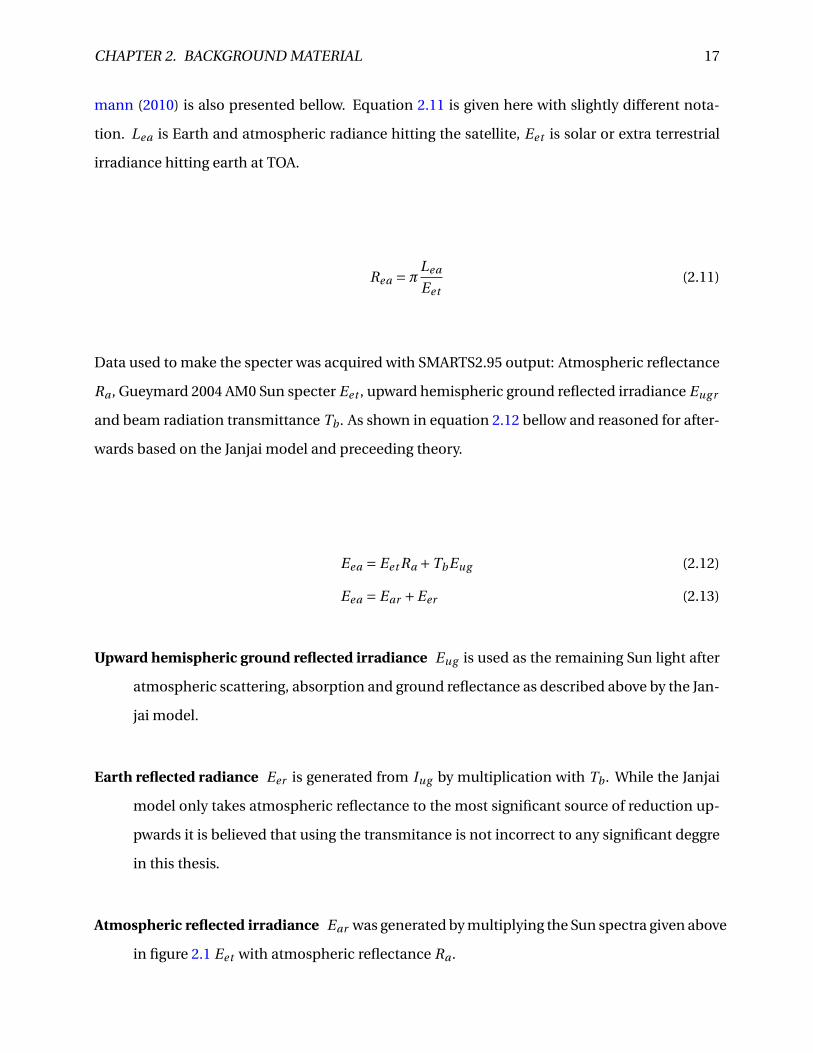


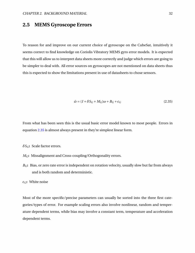


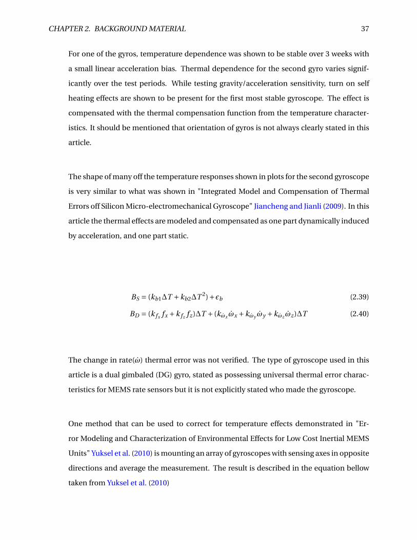


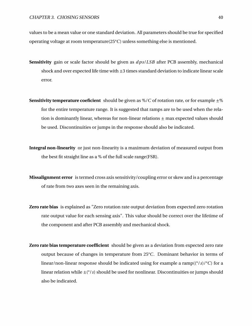


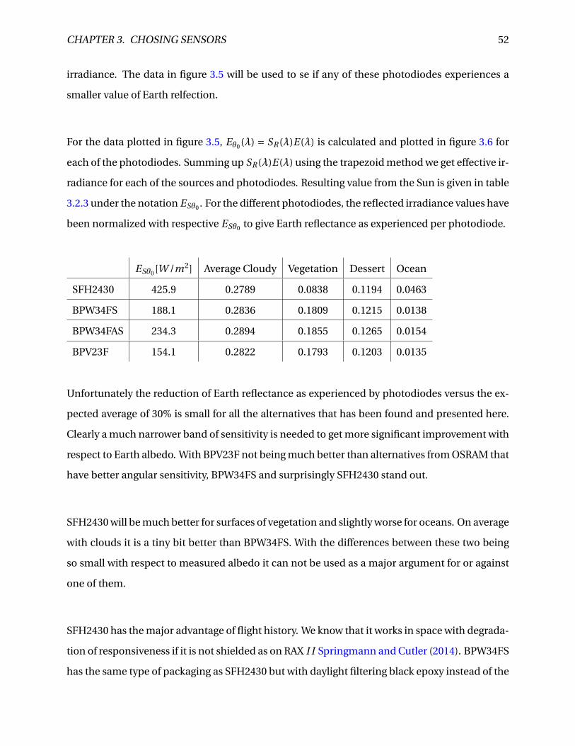


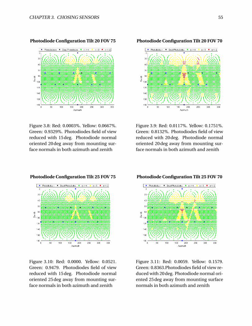


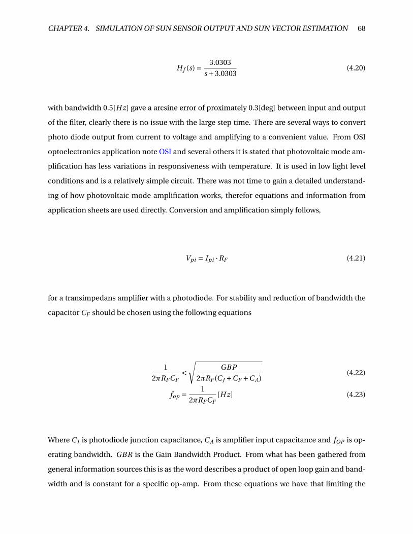


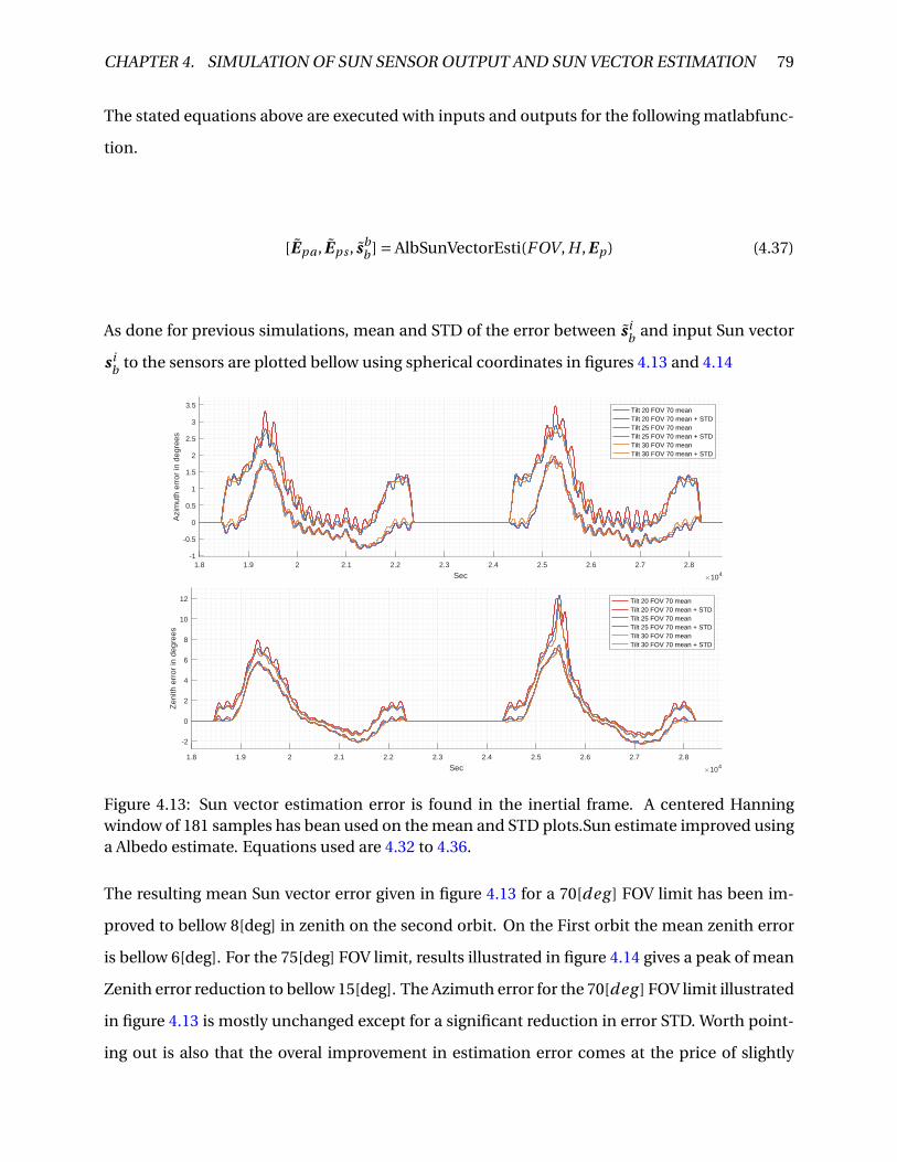


![An overview of Optical Gyroscopes Theory, Practical ... Gyroscopes[1].pdf · An overview of Optical Gyroscopes Theory, Practical Aspects, Applications and Future Trends By Adi Shamir](https://static.documents.pub/doc/80x56/5adedc2a7f8b9ad66b8c1829/an-overview-of-optical-gyroscopes-theory-practical-gyroscopes1pdfan-overview.jpg)
![Control andSelf-Calibrationof MicroscaleRateIntegrating ... · Gyroscopes(FOGs)andintegrated-opticsgyroscopes[16,17]. The operating principle of optical gyroscopes is based on the](https://static.documents.pub/doc/80x56/5fb8aa0c6cc97e21462b9a03/control-andself-calibrationof-microscalerateintegrating-gyroscopesfogsandintegrated-opticsgyroscopes1617.jpg)


