Simulating Zeno Hybrid Systems Beyond Their Zeno Points Haiyang Zheng Electrical Engineering and Computer Sciences University of California at Berkeley Technical Report No. UCB/EECS-2006-114 http://www.eecs.berkeley.edu/Pubs/TechRpts/2006/EECS-2006-114.html September 8, 2006
Transcript
Simulating Zeno Hybrid Systems Beyond Their ZenoPoints
Haiyang Zheng
Electrical Engineering and Computer SciencesUniversity of California at Berkeley
Permission to make digital or hard copies of all or part of this work forpersonal or classroom use is granted without fee provided that copies arenot made or distributed for profit or commercial advantage and that copiesbear this notice and the full citation on the first page. To copy otherwise, torepublish, to post on servers or to redistribute to lists, requires prior specificpermission.
Simulating Zeno Hybrid Systems Beyond Their Zeno Points
by Haiyang Zheng
Research Project
Submitted to the Department of Electrical Engineering and Computer Sciences,
University of California at Berkeley, in partial satisfaction of the requirements for
the degree of Master of Science, Plan II.
Approval for the Report and Comprehensive Examination:
x2 ≤ r2 ∧ x1 > r1}. The set of these two guard sets gives G = {Ge1 , Ge2 , G′e3
, G′e4}.
Finally, R = {Re1 , Re2 , R′e3
, R′e4}, where all reset maps are identity maps.
Now we need to check the completed hybrid system again for possible non-empty
Zeno sets. There are still only two cyclic paths c1 and c2. However by repeating
the above procedure, we get Zc1 = Zc2 = ∅. The detailed derivation process is the
same as described the above and is omitted here. Therefore the completing process
is finished.
In summary we get the completed hybrid system H = ((Q,E), D, G, R, F ), which
is slightly different from the model shown in Fig. 1.4 in that H contains 4 discrete
states. However, if we choose the same dynamics such as (1.1) for discrete states q3
and q4, then q3 and q4 are the same. Thus we get a model with the same dynamics
as that of the model in Fig. 1.4.
2.2.3 Example 3: A Non-Zeno Hybrid System.
Now let us consider a hybrid system simpler than the bouncing ball example
shown in Fig. 1.1. Similar to the bouncing ball example, this hybrid system has a
single state, Q = {q1}, and a single edge, E = {e1}. The set of guards is G = {Ge1},
23
where Ge1 = {x ∈ R | 0 ≤ x ≤ 10}, and the set of the reset maps is R = {Re1},
where Re1 is defined by Re1(x) = x + 1, ∀x ∈ Ge1 .
There is only one element, c = 〈q1; e1; q1〉, in the set C of cyclic paths. For path
c, the composition of reset maps along c is Rc = We1 and πE(c) = e1. Evaluating
equation (2.4) with Zc as the guard Ge1 , we get
Z ′c = Fc(Rn
∞)
= Rc(Rn∞ ∩Ge1)
= We1(Ge1)
= Re1(Ge1) ∩Ge1
= {x ∈ R | 1 ≤ x ≤ 11} ∩ {x ∈ R | 0 ≤ x ≤ 10}
= {x ∈ R | 1 ≤ x ≤ 10}.
Keep evaluating equation (2.4) with Z ′c, and we get
Z ′′c = Fc(Z
′c)
= Rc(Z′c ∩Ge1)
= We1(Z′c)
= Re1(Z′c) ∩ Z ′
c
= {x ∈ R | 2 ≤ x ≤ 10}.
Keep evaluating equation (2.4) with the new results for 10 times, and we will get
Z11c = Fc(Z
10c )
= Rc(Z10c ∩Ge1)
= We1(Z10c )
= Re1(Z10c ) ∩ Z10
c
= Re1({x ∈ R | x = 10}) ∩ {x ∈ R | x = 10}
24
= {x ∈ R | x = 11} ∩ {x ∈ R | x = 10}
= ∅,
where Znc indicates the n-th result from evaluating equation (2.4).
The result set Z11c is an empty set, any set intersecting with an empty set will
result in an empty set. The empty set is the least fixed point of Fc. Because this
fixed point is empty, there is no Zeno point. Therefore, we conclude this model is
non-Zeno and it is already complete.
2.2.4 Example 4: A Zeno Hybrid System.
In this example, we use the same model in Example 2.2.3 but with a different
reset map, R = {Re1}, where Re1 is defined by Re1(x) = x/2, ∀x ∈ Ge1 .
There is only one element, c = 〈q1; e1; q1〉, in the set C of cyclic paths. For path
c, the composition of reset maps along c is Rc = We1 and πE(c) = e1. Evaluating
equation (2.4) with Zc as the guard Ge1 , we get
Z ′c = Fc(Rn
∞)
= Rc(Rn∞ ∩Ge1)
= We1(Ge1)
= Re1(Ge1) ∩Ge1
= {x ∈ R | 0 ≤ x ≤ 5} ∩ {x ∈ R | 0 ≤ x ≤ 10}
= {x ∈ R | 0 ≤ x ≤ 5}.
Keep evaluating equation (2.4) with Z ′c, and we get
Z ′′c = Fc(Z
′c)
= Rc(Z′c ∩Ge1)
25
= We1(Z′c)
= Re1(Z′c) ∩ Z ′
c
= {x ∈ R | 0 ≤ x ≤ 2.5}.
Keep evaluating equation (2.4) with the new results for n times, and we will get
Zn+1c = Fc(Z
nc )
= Rc(Znc ∩Ge1)
= We1(Znc )
= Re1(Znc ) ∩ Zn
c
= Re1({x ∈ R | 0 ≤ x ≤ (1/2)n}) ∩ {x ∈ R | 0 ≤ x ≤ (1/2)n}
= {x ∈ R | 0 ≤ x ≤ (1/2)n+1} ∩ {x ∈ R | 0 ≤ x ≤ (1/2)n}
= {x ∈ R | 0 ≤ x ≤ (1/2)n+1},
where Znc indicates the n-th result from evaluating equation (2.4).
It is obvious that the more times we evaluate the equation (2.4), the bigger n will
be. However, there will not be a limit for n.
Analytically, we can conclude that the least fixed point of Fc is a non-empty set
containing only one element, {0}. However, this result cannot be computed in a finite
number steps. Therefore, our constructive procedure does not work for this kind of
hybrid systems.
2.2.5 Example 5: Another Zeno Hybrid System.
Here is another Zeno hybrid system example, we use the same model in Example
2.2.3 but with a different guard set, Ge1 = {x ∈ R | x ≥ 0}.
There is only one element, c = 〈q1; e1; q1〉, in the set C of cyclic paths. For path
c, the composition of reset maps along c is Rc = We1 and πE(c) = e1. Evaluating
26
equation (2.4) with Zc as the guard Ge1 , we get
Z ′c = Fc(Rn
∞)
= Rc(Rn∞ ∩Ge1)
= We1(Ge1)
= Re1(Ge1) ∩Ge1
= {x ∈ R | x ≥ 1} ∩ {x ∈ R | x ≥ 0}
= {x ∈ R | x ≥ 1}.
Keep evaluating equation (2.4) with Z ′c, we get
Z ′′c = Fc(Z
′c)
= Rc(Z′c ∩Ge1)
= We1(Z′c)
= Re1(Z′c) ∩ Z ′
c
= {x ∈ R | x ≥ 2}.
Keep evaluating equation (2.4) with the new results for n times, we will get
Zn+1c = Fc(Z
nc )
= Rc(Znc ∩Ge1)
= We1(Znc )
= Re1(Znc ) ∩ Zn
c
= Re1({x ∈ R | x ≥ n}) ∩ {x ∈ R | x ≥ n}
= {x ∈ R | x ≥ n + 1} ∩ {x ∈ R | x ≥ n}
= {x ∈ R | x ≥ n + 1},
where Znc indicates the n-th result from evaluating equation (2.4).
27
It is obvious that the more times we evaluate the equation (2.4), the bigger n will
be. However, there will not be a limit for n.
Analytically, noting that R∞ contains ∞, we can conclude that the least fixed
point of Fc is a set containing only one element {∞}. Therefore this system may
have a Zeno behavior, we need to introduce a post-Zeno state for describing the
dynamics after the Zeno point. The completion process is omitted in this report.
However, we have to point out that this fixed point set cannot be computed in a
finite number steps. Therefore, our constructive procedure does not work for this
kind of hybrid systems.
28
Chapter 3
Approximate Simulation
In [11], we proposed an operational semantics for simulating hybrid system models.
The key idea of the operational semantics is to treat a complete simulation as a
sequence of unit executions, where a unit execution consists of two phases. The
discrete phase of execution handles all discrete events at the same time point, and
the continuous phase resolves the continuum between two consecutive discrete events.
When simulating a Zeno hybrid system model, we encounter more challenging
practical issues. The first difficulty is that before the Zeno time point, there will be
an infinite number of discrete transitions (events). Handling a discrete event takes
a non-zero time. So it is impossible to handle all discrete transitions in a finite
time interval. In other words, the simulation gets stuck near the Zeno time point.
The second difficulty is numerical errors, which make it impractical to get an exact
simulation. We will first elaborate on the second issue, and then we will come back
to the first issue in subsection 3.3.
29
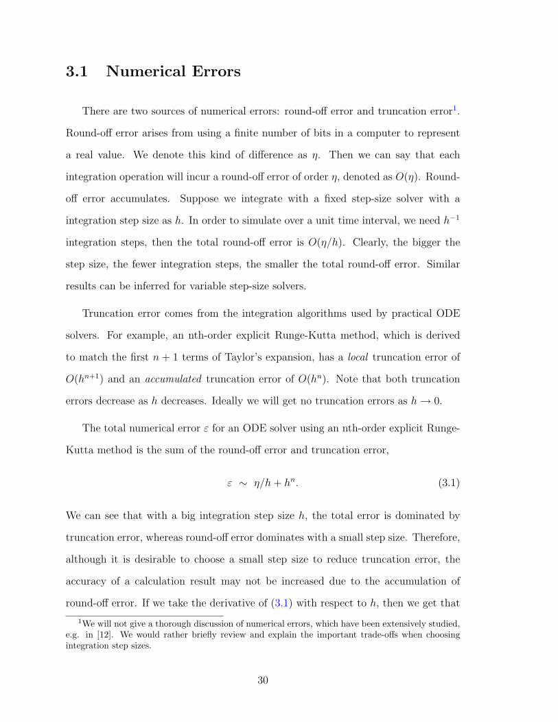
3.1 Numerical Errors
There are two sources of numerical errors: round-off error and truncation error1.
Round-off error arises from using a finite number of bits in a computer to represent
a real value. We denote this kind of difference as η. Then we can say that each
integration operation will incur a round-off error of order η, denoted as O(η). Round-
off error accumulates. Suppose we integrate with a fixed step-size solver with a
integration step size as h. In order to simulate over a unit time interval, we need h−1
integration steps, then the total round-off error is O(η/h). Clearly, the bigger the
step size, the fewer integration steps, the smaller the total round-off error. Similar
results can be inferred for variable step-size solvers.
Truncation error comes from the integration algorithms used by practical ODE
solvers. For example, an nth-order explicit Runge-Kutta method, which is derived
to match the first n + 1 terms of Taylor’s expansion, has a local truncation error of
O(hn+1) and an accumulated truncation error of O(hn). Note that both truncation
errors decrease as h decreases. Ideally we will get no truncation errors as h → 0.
The total numerical error ε for an ODE solver using an nth-order explicit Runge-
Kutta method is the sum of the round-off error and truncation error,
ε ∼ η/h + hn. (3.1)
We can see that with a big integration step size h, the total error is dominated by
truncation error, whereas round-off error dominates with a small step size. Therefore,
although it is desirable to choose a small step size to reduce truncation error, the
accuracy of a calculation result may not be increased due to the accumulation of
round-off error. If we take the derivative of (3.1) with respect to h, then we get that
1We will not give a thorough discussion of numerical errors, which have been extensively studied,e.g. in [12]. We would rather briefly review and explain the important trade-offs when choosingintegration step sizes.
30
when h ∼ η1/(n+1) the total error ε reaches its minimum O(ηn/(n+1)) . Therefore, in
practice, we need to set a lower bound for both the integration step size and error
tolerance (or value resolution) of integration results. We denote them as h0 and ε0
respectively, where
h0 ∼ η1/(n+1), ε0 ∼ ηn/(n+1).
For a good simulation, accuracy is one concern and efficiency is another objective.
Efficiency for numerical integration is usually measured in terms of computation time
or the number of computing operations. Using a big integration step size is an effective
way to improve efficiency but with the penalty of loss of accuracy. So there is a trade-
off. Furthermore, step sizes have upper bounds that are enforced by the consistency,
convergence, and stability requirements when deploying practical integration methods
on concrete ODEs [12]. Therefore, most practical adaptive ODE solvers embed a
mechanism inside the integration process to adjust the step size to meet the desired
tolerance of integration results, so that efficiency gets improved while maintaining the
required accuracy at the same time.
In summary, a practical ODE solver usually specifies a minimum integration step
size h0, some small error tolerance ε0, and an algorithm to adapt step size to meet
requirements on both efficiency and accuracy.
3.2 Computation Difficulties
It is well-known that numerical integration in general can only deliver an approx-
imation to the exact solution of an initial value ODE. However, the distance of the
approximation from the exact solution is controllable for certain kinds of vector fields.
For example, if a vector field satisfies a Lipschitz condition along the time interval
where it is defined, we can constrain the integration results to reside within a neigh-
31
borhood of the exact solution by introducing more bits for representing values to get
better precision and integrating with a small step size.
The same difficulties that arise in numerical integration also appear in event detec-
tion. A few algorithms have been developed to solve this problem [13]–[15]. However,
there is still a fundamental unsolvable difficulty: we can only get the simulation time
close to the time point where an event occurs, but we are not assured of being able
to determine that point precisely.
Simulating a Zeno hybrid system poses another fundamental difficulty. We will
first explain it through a simple continuous-time example with dynamics
x(t) = 1/(t− 1), x(0) = 0, t ∈ [0, 2]. (3.2)
We can analytically find the solution for this example, x(t) = ln |t − 1|. However,
getting the same result through simulation is difficult. Suppose the simulation starts
with t = 0. As t approaches 1, the derivative x(t) keeps decreasing without bound. To
satisfy the convergence and stability requirements, the step size h has to be decreased.
When the step size becomes smaller than h0, round-off error is not neglectable any
more and the simulation results become unreliable. Trying to reduce the step size
further doesn’t help, because the disturbance from round-off error will dominate.
A similar problem arises when simulating Zeno hybrid system models. Recall that
Zeno executions have an infinite number of discrete events (transitions) before reach-
ing the Zeno time point, and the time intervals between two consecutive transitions
shrink to 0. When the time interval becomes less than h0, round-off errors again
dominate.
In summary, it is impractical to precisely simulate the behavior of a Zeno model.
Therefore, similar to numerical integration, we need to develop a computationally
feasible way to approximate the exact model behavior. The objective is to give a
32
close approximation under the limits enforced by numerical errors. We will do this in
the next subsection.
3.3 Approximating Zeno Behaviors
In Sect. 2, we have described how to specify the behaviors of a Zeno hybrid system
before and after the Zeno time point and how to develop transitions from pre-Zeno
states to post-Zeno states. The construction procedure works for guards which are
arbitrary sets. However, assuming that each guard is the sub-levelset of a function
(or collection of functions) simplifies the framework for studying transitions to post-
Zeno states. Therefore, we assume that a transition going from a pre-Zeno state to a
post-Zeno state has a guard expression of form,
Gec = {x ∈ Rn∞ | gec(x) ≤ 0}, (3.3)
for every c ∈ C, where ec = h−1(c) and gec : Rn∞ → Rk
∞. Furthermore, we assume
that gec(x) is continuously differentiable.
In this section, we will develop an algorithm such that the complete model behav-
ior can be simulated. As the previous subsection pointed out, we can only approximate
the model behaviors before the Zeno time point. Therefore, the first issue is to be
able to tell how close the simulation results are to the exact solutions before the Zeno
time point. This will decide when the transitions from pre-Zeno states to post-Zeno
states are taken. The second issue is how to establish the initial conditions of the
dynamics after the Zeno time point from the approximated simulation results.
33
3.3.1 Issue 1: Relaxing Guard Expressions.
To solve the first issue, we first relax the guard conditions defining the transitions
from the pre-Zeno states to the post-Zeno states; if the current states fall into a
neighborhood of the Zeno states (the states at the Zeno time point), the guard is
enabled and transition is taken. Note that when the transition is taken, the system
has a new dynamics and the rest of the events before the Zeno time point, which are
infinite in number, are discarded. Therefore the computation before the approximated
Zeno time point can be finished in finite time.
A practical problem now is to define a good neighborhood such that the approxi-
mation is “close enough” to the exact Zeno behavior. We propose two criteria. The
first criterion is based on the error tolerance ε02. We rewrite (3.3) as
Gε0ec
= {x ∈ Rn∞ | gec(x) ≤ ε0}, (3.4)
meaning if x(t) is the solution of x = fq(x) with q = s(ec), and if the evaluation
result of gec(x(t)) falls inside [0, ε0], the simulation results of x(t) will be thought as
close enough to the exact solution at the Zeno time point, and the transition will be
taken. In fact, because ε0 is the smallest amount that can be reliably distinguished,
any value in [0, ε0] will be treated the same.
The second criterion is based on the minimum step size h0. Suppose the evaluation
result of gec(x(t)) is outside of the range [0, ε0]. If it takes less than h0 time for the
dynamics to drive the value of gec(x(t)) down to 0, then we will treat the current states
as close enough to the Zeno states. This criterion prevents the numerical integration
from failing with a step size smaller than h0, which may be caused by some rapidly
changing dynamics, such as those in (3.2).
2If gec(x) is a vector valued function, then ε0 is a vector with ε0 as the elements.
34
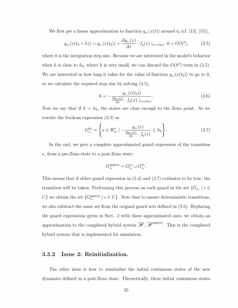
We first get a linear approximation to function gec(x(t)) around t0 (cf. [13], [15]),
gec(x(t0 + h)) = gec(x(t0)) +∂gec(x)
∂x· fq(x) |x=x(t0) ·h + O(h2), (3.5)
where h is the integration step size. Because we are interested in the model’s behavior
when h is close to h0, where h is very small, we can discard the O(h2) term in (3.5).
We are interested in how long it takes for the value of function gec(x(t0)) to go to 0,
so we calculate the required step size by solving (3.5),
h = − gec(x(t0))∂gec (x)
∂x· fq(x) |x=x(t0)
. (3.6)
Now we say that if h < h0, the states are close enough to the Zeno point. So we
rewrite the boolean expression (3.3) as
Gh0ec
=
{x ∈ Rn
∞ | − gec(x)∂gec (x)
∂x· fq(x)
≤ h0
}. (3.7)
In the end, we give a complete approximated guard expression of the transition
ec from a pre-Zeno state to a post-Zeno state:
Gapproxec
= Gε0ec∪Gh0
ec.
This means that if either guard expression in (3.4) and (3.7) evaluates to be true, the
transition will be taken. Performing this process on each guard in the set {Gec | c ∈
C} we obtain the set {Gapproxec
| c ∈ C}. Note that to ensure deterministic transitions,
we also subtract the same set from the original guard sets defined in (2.6). Replacing
the guard expressions given in Sect. 2 with these approximated ones, we obtain an
approximation to the completed hybrid system H , Happrox
. This is the completed
hybrid system that is implemented for simulation.
3.3.2 Issue 2: Reinitialization.
The other issue is how to reinitialize the initial continuous states of the new
dynamics defined in a post-Zeno state. Theoretically, these initial continuous states
35
are just the states at the Zeno time point, meaning that they satisfy the guard
expression in (3.3). This is guaranteed by the identity reset maps associated with
the transitions.
In some circumstances, like the examples discussed in this report, the initial con-
tinuous states can be explicitly and precisely calculated. However, in general, if there
are more variables involved in guard expressions than the constraints enforced by
guard expressions, we cannot resolve all initial states. In this case, we have to use the
simulation results as part of the initial states. Clearly, since in simulation we do not
actually reach the Zeno time point, the initial states are just approximations. Con-
sequently, the simulation of the dynamics of post-Zeno states will be approximation
too.
36
Chapter 4
Conclusion
In this report, a systematic method is introduced for completing hybrid systems
through the introduction of new post-Zeno states and transitions to these states at
the Zeno point. A way to approximate model behaviors at Zeno points is developed
such that the simulation does not halt nor break down. With these solutions, a Zeno
hybrid system model can be simulated beyond its Zeno point and its dynamics is
revealed completely.
37
References
[1] J. Zhang, K. H. Johansson, J. Lygeros, and S. Sastry, “Zeno hybrid systems,” Int. J. Robust
and Nonlinear Control, vol. 11, no. 2, pp. 435–451, 2001.
[2] A. D. Ames, A. Abate, and S. Sastry, “Sufficient conditions for the existence of zeno behavior,”
in 44th IEEE Conference on Decision and Control and European Control Conference ECC,
2005.
[3] A. D. Ames, P. Tabuada, and S. Sastry, “On the stability of Zeno equilibria,” in Hybrid Systems:
Computation and Control (HSCC), J. P. Hespanha and A. Tiwari, Eds., vol. LNCS 3927. Santa
Barbara, CA, USA: Springer-Verlag, 2006, pp. 34 – 48.
[4] K. H. Johansson, J. Lygeros, S. Sastry, and M. Egerstedt, “Simulation of zeno hybrid au-
tomata,” in Proceedings of the 38th IEEE Conference on Decision and Control, Phoenix, AZ,
1999.
[5] A. D. Ames and S. Sastry, “Blowing up affine hybrid systems,” in 43rd IEEE Conference on
Decision and Control, 2004.
[6] P. J. Mosterman, “An overview of hybrid simulation phenomena and their support by simulation
packages,” in Hybrid Systems: Computation and Control (HSCC), F. Varager and J. H. v.
Schuppen, Eds., vol. LNCS 1569. Springer-Verlag, 1999, pp. 165–177.
[7] A. D. Ames, H. Zheng, R. Gregg, and S. Sastry, “Is there life after zeno? taking executions
past the breaking (zeno) point,” in American Control Conference (ACC), 2006.
[8] A. van der Schaft and H. Schumacher, An Introduction to Hybrid Dynamical Systems, ser.
Lecture Notes in Control and Information Sciences 251. Springer-Verlag, 2000.
[9] J. Lygeros, Lecture Notes on Hybrid Systems. ENSIETA 2-6/2/2004, 2004.
[10] B. A. Davey and H. A. Priestley, Introduction to Lattices and Order, 2nd ed. Cambridge
University Press, 2002.
[11] E. A. Lee and H. Zheng, “Operational semantics of hybrid systems,” in Hybrid Systems: Com-
putation and Control (HSCC), M. Morari and L. Thiele, Eds., vol. LNCS 3414. Zurich,
Switzerland: Springer-Verlag, 2005, pp. pp. 25–53.
[12] R. L. Burden and J. D. Faires, Numerical analysis, 7th ed. Brroks/Cole, 2001.
[13] L. F. Shampine, I. Gladwell, and R. W. Brankin, “Reliable solution of special event location
problems for odes,” ACM Trans. Math. Softw., vol. 17, no. 1, pp. 11–25, 1991.
38
[14] T. Park and P. I. Barton, “State event location in differential-algebraic models,” ACM Trans-
actions on Modeling and Computer Simulation (TOMACS), vol. 6, no. 2, pp. 137–165, 1996.
[15] J. M. Esposito, V. Kumar, and G. J. Pappas, “Accurate event detection for simulating hybrid
systems,” in Hybrid Systems: Computation and Control (HSCC), vol. LNCS 2034. London,