Simulation and Measurement of Non-Functional Properties of ...

Degree project

Simulation and Measurement of Non-Functional Properties of Web Services in a Service Market to Improve User Value

Author: Catherine Catherine Supervisor: Welf Löwe External Supervisor: Jens Kirchner, Karlsruhe University of Applied Sciences Date: 2013-12-31 Course Code: 5DV01E, 15 credits Level: Master Department of Computer Science

i

Abstract In a Service Oriented Architecture, information systems are composed of different individual services. This is comparable to Lego bricks, which can be arbitrary combined with other bricks.

In the context of Service Oriented Computing, the Internet is becoming a market of services, in which providers and consumers meet each other. In this case, it could happen that multiple vendors provide the same service functionality. This condition makes it difficult for the consumers to select the provider which best fulfils his requirements and needs. Nevertheless, the existing service varieties distinguish themselves in their non-functional characteristics, such as response time, availability or costs.

As part of the joint research project of the Karlsruhe University of Applied Sciences and the Linnaeus University in Växjö, Sweden, a framework is developed which automatically binds service consumers to their best-fit service providers based on non-functional properties and consumers’ requirements.

This form of service market stands currently in the emerging development process which is conspicuous in a rapidly growing Internet world. This work aims for the validation whether the application of the developed framework in such a market would bring additional value for service consumers. For this purpose, a simulation environment is created, in which a futuristic service market is projected. Within the simulation environment, network communication for service invocation scenario is simulated based on a simplified model. The goal is to manipulate the measured non-functional properties of services like response time and availability to mimic real world scenario. Keywords: Service Oriented Computing, Service Oriented Architecture, services, framework, simulation

Disclaimer This work is done under supervision of researchers at Karlsruhe University of Applied Sciences, Germany and Linnaeus University, Växjö, Sweden. The report is therefore presented and published at both places.

ii

Table of Content

1 Introduction ........................................................................................................ 1 1.1 Service Oriented Architecture .............................................................................................. 1

1.2 Problem Definition ............................................................................................................... 1

1.3 Framework of Service Oriented Computing ........................................................................ 2 1.3.1 Motivation and Project Background ................................................................................. 2 1.3.2 Framework Approach ....................................................................................................... 2 1.3.3 Framework Architecture ................................................................................................... 3

1.4 Objective of the Thesis ......................................................................................................... 4

1.5 Report Layout ....................................................................................................................... 5

2 Background ........................................................................................................ 6 2.1 Discrete Event Simulation .................................................................................................... 6

2.2 General Simulation System .................................................................................................. 7 2.2.1 DESMO-J ......................................................................................................................... 7 2.2.2 J-Sim (Java Simulator) ..................................................................................................... 8

2.3 Network Simulation .............................................................................................................. 9 2.3.1 WANem (Wide Area Network Emulator) ........................................................................ 9 2.3.2 NS2 (Network Simulator version2) ................................................................................ 10 2.3.3 OPNET (Optimized Network Engineering Tool) Modeler ............................................ 11

2.3.4 OMNET++ (Optical Micro-Networks Plus Plus)........................................................... 11

2.3.5 NIST Net (Network Emulation Tool)............................................................................. 12

3 Architectural Design ........................................................................................ 14 3.1 Construction of Existing Framework ................................................................................. 14

3.2 Architecture Concept of Simulation Environment ............................................................. 14 3.2.1 Full Virtualization using Virtual Machines .................................................................... 14 3.2.2 Virtual Hosting using distinct ESB Instances ................................................................ 16

4 Simulation Design and Concept ....................................................................... 19

4.1 Non-functional Characteristics of Services ........................................................................ 19 4.1.1 Response Time ............................................................................................................... 19 4.1.2 Availability ..................................................................................................................... 20

4.1.3 Throughput ..................................................................................................................... 21 4.1.4 Reliability ....................................................................................................................... 21

4.2 Implementation concept ..................................................................................................... 21 4.2.1 Interception of the Simulator .......................................................................................... 22 4.2.2 Simulating Response Time ............................................................................................. 23 4.2.3 Simulating Availability .................................................................................................. 25

5 Implementation ................................................................................................ 27 5.1 The Simulator as Java Servlet ............................................................................................ 27

5.2 Simulating Response Time ................................................................................................. 29

iii

5.3 Simulating Availability ...................................................................................................... 30

6 Experiment and Evaluation .............................................................................. 32

6.1 Test Scenario ...................................................................................................................... 32

6.2 Evaluation ........................................................................................................................... 32

7 Conclusion ........................................................................................................ 38 7.1 Summary............................................................................................................................. 38

7.2 Future Work........................................................................................................................ 39

References ............................................................................................................ 40

Apendix A Detailed Validation Results ............................................................... 44

iv

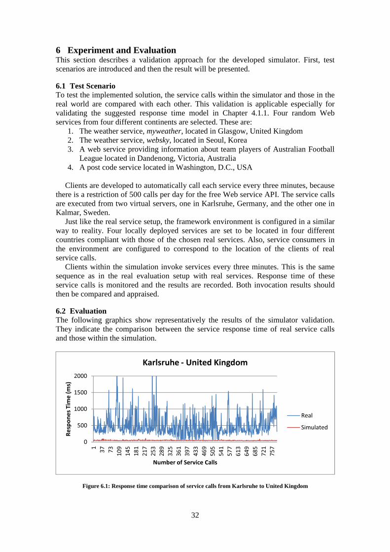
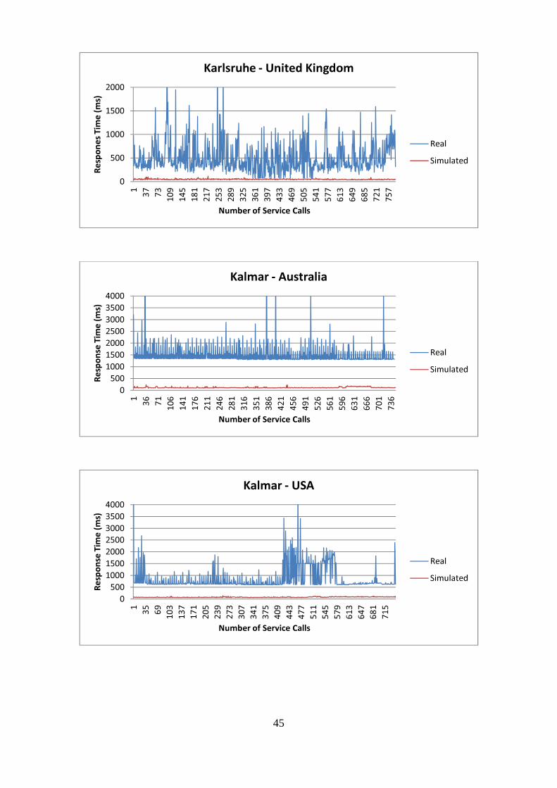
List of Figures Figure 1.1: SOC Framework Architecture (Kirchner et al., 2011) ................................... 4 Figure 2.1: Configuration options of WANem ............................................................... 10 Figure 3.1: Current system construction......................................................................... 14 Figure 3.2: System Architecture for Virtualization of Integration Environment ........... 15 Figure 3.3: Architecture for Virtualization of Integration Platform ............................... 17 Figure 4.1: Request Flow in SOC Framework ............................................................... 22 Figure 4.2: Web Proxy Server (Schnabel, 2004) ............................................................ 22 Figure 4.3: Request passing the simulator ...................................................................... 23 Figure 4.4: Additional headers in SOAP message ......................................................... 24 Figure 4.5: Service response flow .................................................................................. 24 Figure 5.1: Sequence diagram of response time simulation ........................................... 30 Figure 6.1: Response time comparison of service calls from Karlsruhe to United Kingdom ......................................................................................................................... 32 Figure 6.2: Response time comparison of service calls from Kalmar to United Kingdom ........................................................................................................................................ 33 Figure 6.3: Response time comparison of service calls from Karlsruhe to Korea ......... 33

Figure 6.4: Response time comparison of service calls from Kalmar to Korea ............. 33 Figure 6.5: Network as a graph (based on Peterson and Davie, 2011) ......................... 35

Figure 6.6: Comparison between time for ping calls and simulation from Kalmar to Korea .............................................................................................................................. 35 Figure 6.7: Comparison between time of ping calls and simulation from Kalmar to United Kingdom ............................................................................................................. 36 Figure 6.8: Response time comparison of service calls within simulation .................... 36

Figure 6.9: Comparison of simulated service availability with the same availability value ............................................................................................................................... 37

v

List of Abbreviations ACA Autonomous Component

Architecture API Application Programming

Interface Bps Bits per Second DARPA Defense Advanced Research

Projects Agency DES Discrete Event

Simulation/Simulator DESMO-J DES Modelling in Java ESB Enterprise Service Bus GUI Graphical User Interface HTTP Hypertext Transfer Protocol IC Integrated Circuit ICV Intelligent Collaboration and

Visualisation J-Sim Java Simulator JVM Java Virtual Machine MTU Maximum Transmission Unit MURI/AFOSR Air Force Office of

Scientific Research’s Multidisciplinary University Research Initiative

NAM Network Animator NED Network Description NF non-functional

NIST National Institute of Standards and Technology

NIST Net Network Emulation Tool from NIST

NMS Network Measurement and Simulation

NS2 Network Simulator version2 NSF National Science Foundation OMNET++ Optical Micro Network

Plus Plus OPNET Optimized Network

Engineering Tool OS Operating System OTcl Object-oriented Tool Command

Language QoS Quality of Service SL Service Level SLA Service Level Agreements SOA Service Oriented Architecture SOAP Simple Object Access Protocol SOC Service Oriented Computing Tcl Tool Command Language VM Virtual Machine WAN Wide Area Network WANem Wide Area Network Emulator XML Extensible Markup Language

1

1 Introduction This chapter provides background information about the research project in the field of Service Oriented Computing and framework which is developed within the project and is basis of this work. Afterwards, the aim of the thesis will be presented.

1.1 Service Oriented Architecture IT-Systems form the base of almost all business processes, no matter of the affected products, market sections, and enterprise sizes. Typical enterprise software performs a large range of functionality that consists of a set of functions that are parameterised and combined in a task-specific manner.

To allow an efficient development and high flexibility for reacting on changing requirements, those functions, called services, can be deployed independently of each other. The combination of those services to software that supports full business processes is called Service Oriented Computing (SOC) / Service Oriented Architecture (SOA).

SOC focuses on the development of software solutions based on services that use standard technologies.

“A primary goal of SOC is to make a collection of software services accessible via standardized protocols, whose functionality can be automatically discovered and integrated into applications or composed to form more complex services.”

(Bichier and Lin, 2006) The implementation of such models relies on the SOA. SOA is an architectural

approach to build software systems based on loosely coupled components (Weerawarana, 2005). This kind of system design provides flexibility and allows enterprise wide reusability of the systems or services (Krafzig et al., 2005). The usage of SOA services is platform independent, i.e. clients are not limited to use specific hardware or software platforms to invoke the services. As standardised technologies are used to implement these services and standardised interfaces are used for the interaction of services, the concrete implementation of a service becomes less important. Instead, the service can be performed by any implementation that provides the required functionality and obeys the interface definition. This makes implementations exchangeable.

Georgakopoulos and Papazoglou (2008) argue that Web services have become the preferred implementation technology of realising SOA. Technologies used to develop Web services are e.g. HTTP, SOAP or XML. There are three major components in the web service architecture: service provider, service registry, and service consumer. Service providers publish their services’ definition to a service registry hosted by a service discovery agent (service broker) like UDDI (Papazoglou, 2008). Service consumers search for providers with corresponding services in the service registry. Discovery agents then respond to the consumer by giving some information about the service providers, the service description. Finally, service consumers use the provided information to establish contact with a service provider and invoke the service (Papazoglou, 2003).

1.2 Problem Definition In the past years, the number of available services on the internet has increased. As a consequence, the same service functionality is offered by multiple providers. This situation makes it difficult for service consumers to choose the right service provider that best fits the consumer’s functional and non-functional (NF) requirements. As many

2

providers offer the same functionality, the consumer must rely on NF requirements to choose the right service. Therefore Georgakopoulos and Papazoglou (2008: 192) point out that there is a need for consumers to be able to distinguish the services on the basis of their NF properties such as quality of service (QoS). They define QoS as a set of quantitative (e.g. response time and price) and qualitative (e.g. reliability and reputation) characteristics of a service which correlates service delivery with consumer requirements.

For example, a consumer from Sweden preferably uses a service also located in Sweden due to its geographical proximity. But since the consumer invokes the service during lunch time, which is the service’s busiest time in this scenario, not each request can be processed in time. The consumer decides to call another service provider, which offers the same functionality, but is located in America. Hence the different time zone, the service workload is lower at the given invocation time, i.e. the response time to call services in America is shorter than to invoke services in Sweden within the specific time frame.

NF properties of services are up to now defined in the so called Service Level Agreements (SLA), which service consumers need to rely on during the decision process of choosing a service instance. Due to the fact that service providers want to sell their services profitably, they tend to describe their services in SLA better than they actually are (Kirchner et al., 2011). For the consumer this leads to the questions, which of the available services provides both the required logic as well as the required NF requirements in a reliable manner.

To eliminate this issue, a study was conducted within a research project to measure and analyse the NF characteristics of services. This study results in a development of a framework which helps service consumers in finding their best-fit service provider based on the NF properties of services. Next section gives an overview about this framework.

1.3 Framework of Service Oriented Computing This following section describes a framework developed within a joint research project in SOC field, which is the basis of this thesis.

1.3.1 Motivation and Project Background A joint research project of the Karlsruhe University of Applied Sciences and the Linnaeus University in Växjö, Sweden, has shown that NF properties of services such as response time can vary from time to time (Kirchner et al., 2011). Therefore, “the created static SLAs do not always reflect the current NF characteristics of a service” (Kirchner et al., 2011). A decision based solely on the information provided by the providers themselves is not a reliable basis for the selection of the best-fit services. Within this research project, a framework has been developed that will serve as a remedy to evaluate and compare the NF characteristics of different service providers from the service consumer’s point of view. It should help service consumers in finding and selecting service providers, which can best fulfil their requirements.

1.3.2 Framework Approach The developed framework intends to steadily select the most suitable service provider for each consumer and to ensure improved QoS. The measurement of the NF properties is performed every time the service is used, which is why the decision regarding the service binding adapts dynamically to the changing environment and different quality of service providers. In addition to the NF properties of service providers, the selection of best-fit service also depends on the service consumer context (e.g. service call time,

3

consumer location, etc.) and consumer utility (i.e. weighted quality goals) (Kirchner et al., 2011).

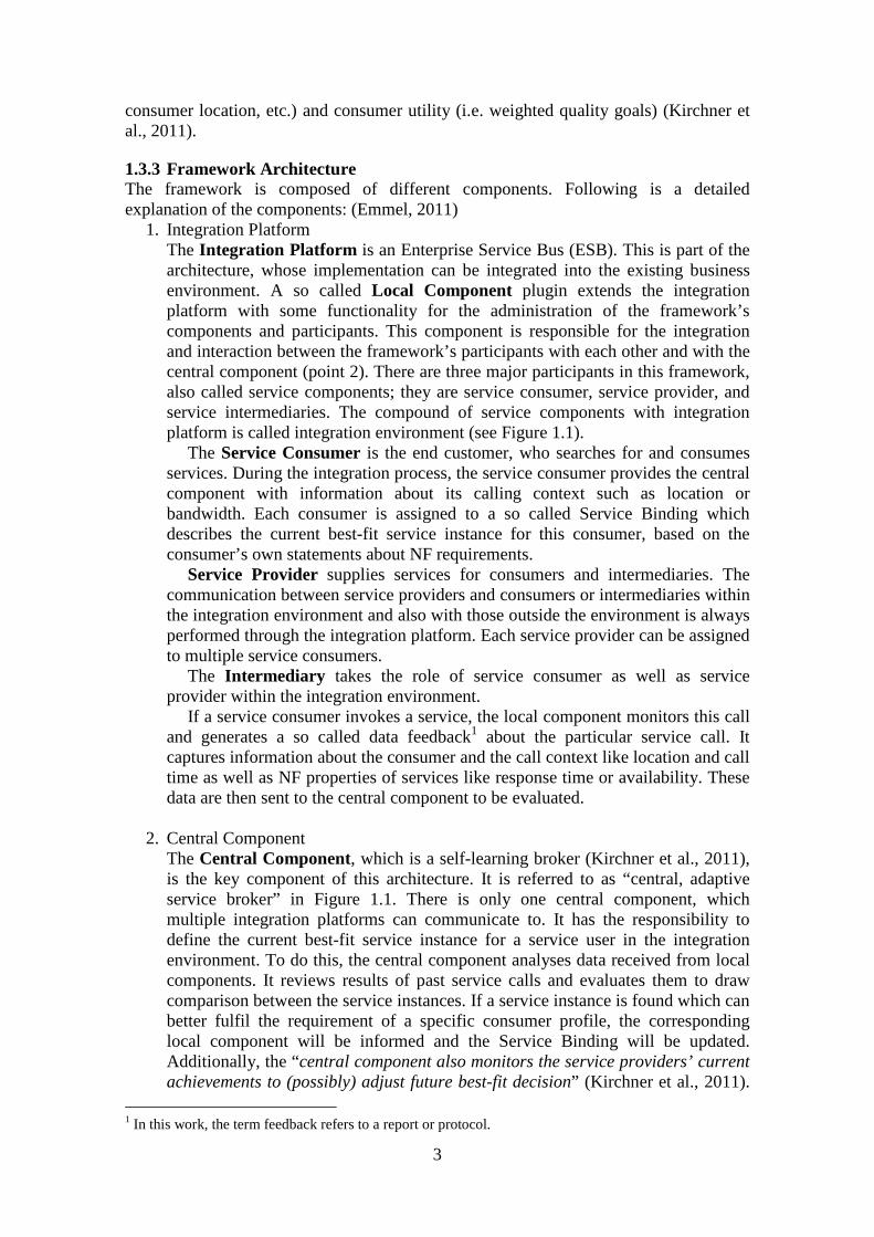
1.3.3 Framework Architecture The framework is composed of different components. Following is a detailed explanation of the components: (Emmel, 2011)

1. Integration Platform The Integration Platform is an Enterprise Service Bus (ESB). This is part of the architecture, whose implementation can be integrated into the existing business environment. A so called Local Component plugin extends the integration platform with some functionality for the administration of the framework’s components and participants. This component is responsible for the integration and interaction between the framework’s participants with each other and with the central component (point 2). There are three major participants in this framework, also called service components; they are service consumer, service provider, and service intermediaries. The compound of service components with integration platform is called integration environment (see Figure 1.1).

The Service Consumer is the end customer, who searches for and consumes services. During the integration process, the service consumer provides the central component with information about its calling context such as location or bandwidth. Each consumer is assigned to a so called Service Binding which describes the current best-fit service instance for this consumer, based on the consumer’s own statements about NF requirements.

Service Provider supplies services for consumers and intermediaries. The communication between service providers and consumers or intermediaries within the integration environment and also with those outside the environment is always performed through the integration platform. Each service provider can be assigned to multiple service consumers.

The Intermediary takes the role of service consumer as well as service provider within the integration environment.

If a service consumer invokes a service, the local component monitors this call and generates a so called data feedback1 about the particular service call. It captures information about the consumer and the call context like location and call time as well as NF properties of services like response time or availability. These data are then sent to the central component to be evaluated.

2. Central Component The Central Component, which is a self-learning broker (Kirchner et al., 2011), is the key component of this architecture. It is referred to as “central, adaptive service broker” in Figure 1.1. There is only one central component, which multiple integration platforms can communicate to. It has the responsibility to define the current best-fit service instance for a service user in the integration environment. To do this, the central component analyses data received from local components. It reviews results of past service calls and evaluates them to draw comparison between the service instances. If a service instance is found which can better fulfil the requirement of a specific consumer profile, the corresponding local component will be informed and the Service Binding will be updated. Additionally, the “central component also monitors the service providers’ current achievements to (possibly) adjust future best-fit decision” (Kirchner et al., 2011).

1 In this work, the term feedback refers to a report or protocol.

4

The central component is developed as a Web service running on an application server.

Figure 1.1: SOC Framework Architecture (Kirchner et al., 2011)

1.4 Objective of the Thesis This framework addresses a currently emerging service market, whose final form is still in the development. It is uncertain whether the application of this framework would offer added value and indeed bring improvements in a certain way. Therefore a test environment is required, which can sufficiently picture the environment of service markets in the future and enables the validation of the developed framework. To obtain useful results, the validation process must be performed in various realistic scenarios, i.e. as mentioned before, that NF properties of services are not static performance indicators, but their values may change from time to time depending on several factors. The simulation environment should be developed to reproduce this kind of scenario, i.e. simulation should be able to control or manipulate NF properties of services with regards to realistic factors.

The simulation environment should become a component of the existing framework environment described in the previous section and provide the capability to simulate generic network characteristic of service calls. Realistic means that the determining factors, created in the simulation, should comply with the one in reality. This includes delay or jitter during service request transmissions, services outages, services overloads, dropped service calls when bandwidth exceeds, and variable service response time depending on aspects like bandwidth, invocation time and other factors.

Distinct services behave differently in various network environments. Service instance characteristics like provider location or utilisation rate are not the only influencing factors in measuring NF properties, but also consumer context such as

Integration Platform Service

Components

Integration

Environment

5

bandwidth or time of call. The simulator should observe those properties and facilitate the configuration of these extents for each service component. In this way, various scenarios can be created during the simulation process.

Moreover, considering that there are a huge number of factors or conditions affecting the behaviour of services in a real world scenario the simulation environment is built in a controlled manner. It is desirable to create a reproducible world within the simulation. Reproducible means that service calls under identical conditions can be reproduced to generate similar measurement results with a moderate deviation. To achieve this, a good understanding of the implementation of the simulation environment is necessary so that the desired outcome is verifiable.

By this means, service request traffic with varied settings can be produced, local components can capture data feedback, which afterwards can be forwarded to the central component and used to verify the framework using machine learning and data mining approaches.

In conclusion, the simulation system should be a stand-alone component which can be assembled to be part of the SOC framework without affecting the function of each framework component and participant. Following goal criteria should be considered in developing the simulation system:

1. The simulation system could be integrated to the existing laboratory SOC framework environment.

2. The simulation system could be easily detached from the framework environment.

3. The simulation system could realistically simulate NF properties of services such as response time, availability, etc.

4. User of the simulation system should be provided with graphical user interface to able to configure different input parameters for the execution of the simulation process.

5. Simulation results of NF properties of services could vary depending on defined model and input parameters.

1.5 Report Layout This thesis is organised as follows. The next chapter gives an overview about the background in the simulation area, general service simulation as well as network simulation. In Chapter 3, the architecture of the existing framework will be introduced and ideas about building simulation environments based on the existing architecture design are contributed. Also the decision to create an own simulation software is explained. Chapter 4 gives an overview of NF characteristics which should be simulated. Then, concepts to simulate the selected NF properties are exhibited. Knowledge about the implementation of introduced concepts is presented in Chapter 5 and validation of the developed solution in Chapter 6. The last chapter concludes this work and suggests possible improvements for the future work.

6

2 Background Simulation techniques have been applied and developed in different research fields. Hartmann (2005) argues that research cannot be imagined without simulation and almost each academic discipline has at least a little use for simulations. In science and engineering, simulations are used to recreate a real-world system. Real-world systems are in most cases too complex to allow recreating realistic models for evaluation purpose. Therefore, computer simulation is a convenient way to evaluate a model of a real system (Law, 2000). Hartmann (2005) introduces five motivations of running simulation:

1. Technique: Simulations allow researchers to investigate the detailed dynamic of a real system and to obtain very accurate answers to the questions of interest.

2. Heuristic tools: “Simulations have a major role in the process of developing hypotheses, models and new theories.”

3. Substitution for an experiment: Simulations allow researchers to perform impossible experiments, e.g. study the formation of galaxies.

4. Tool for experimentalists: Simulations support experiments. 5. Pedagogical tool: Simulations can help students in understanding an underlying

process during learning.

In the SOC context, service vendors create simulation models of the offered services to verify their functionality before the release. The vendors have the possibility to address feasible issues before these become problems (Chandrasekaran et al., 2002). Miller et al. (2002) also argues that since flexibility is one of the requirements for the competitiveness on the open market, simulation can serve for the purpose of service design correction and improvement as well as adaptive changes at runtime. Considering that the success of organisations depends on efficiency and effectiveness of its business processes and that most business processes are implemented by combining services, it is useful to analyse the overall structure and functionality as well as the NF characteristic of the services (Chandrasekaran et al., 2002). Simulation of NF aspects will respond to “what-if” questions during the process design and help in investigating how composed web services will perform when they are deployed (Chandrasekaran et al., 2002).

This chapter points out some examples of service simulation systems and environment for the purpose of (non-)functionality validation, correction, and improvement. Furthermore, some network simulators are introduced to be used in the QoS analysis. The next section gives a short introduction about discrete event simulation, based on which most simulation technologies are developed.

2.1 Discrete Event Simulation In order to simulate something, an appropriate model is required. A model usually contains several systems that are themselves models of logic that represents behaviour and variables that represent the state of the model. The process of simulation is usually the initialisation of the variables followed by either manual or automated change of a given variable and the observation of how the other variables change in reaction.

According to Banks et al. (2005), discrete event simulation (DES) is a modelling methodology of systems in which the state variable changes only at a discrete set of points in time. “The state of a system is a collection of variables necessary to describe a system at any time” (Banks et al., 2010: 30). A possible state variable in production system is for example the status of machines (busy, down, etc.). A system is composed of a number of entities. Entities are system components, e.g. server, machine, etc. Each

7

entity has attributes, which are part of the system state. If a production machine is the entity, its attribute could be the machines’ status (busy or idle). (Law, 2007)

The changes of these variables are organised in terms of events (Göbel, 2006). Events occur instantaneously and may change the state of the system (Law, 2007), e.g. breakdown of a production machine. Events are processed sequentially. The completion of one event may trigger the start of another event (event routine). Future events are stored in an event list (Buss, 2002). If two or more events are scheduled at the same time, a rule is required to determine which event is to be executed first (Buss, 2002), like for example by prioritising the event based on the execution time.

Simulation processes usually start at fictional time T by initialising the required parameters, such as the simulation clock (value of simulated time), state variables, statistical counters (which contain information about the system performance for statistical report purpose at the end of the simulation), and the event list (a list of future events). Data and events are often relative to the time T, for example the simulated bandwidth utilisation over time. Banks et al. (2010) recommends that the event list is ordered by event time, i.e. events are arranged chronologically. The determination of future events is therefore based on the event list. If the next event to occur is associated with t1, the simulation clock is advanced to the time t1, and the event is executed. During this time, some activities occur, like for example updates of the state variables, gathering of information about the system performance or establishment of the following next events. If another future event is found, the process is repeated until stopping circumstances arise. If termination should be processed, statistical counters are analysed and a simulation report will be generated. Each finished event will then be removed from the event list. (Law, 2007; Banks et al., 2010)

The main focus in this thesis is network simulation, because, as explained in Chapter 3, this is the only simulated resource that does not exist as part of the framework.

2.2 General Simulation System In the following section, some simulation environments are described representatively.

2.2.1 DESMO-J Information about DESMO-J in this section is based on Page and Kreutzer, 2005. DESMO-J (DES Modelling in Java) is a Java-based development framework for DES modelling. It contains a library of reusable classes for simulation experiments. It was developed at the University of Hamburg and is available as free and open-source software under the Apache License, Version 2.0.

DESMO-J is divided into two major components. Using a so-called black box framework, a number of pre-defined components can be easily chosen, used, and suitably instantiated. Domain experts with basic programming skills should be able to integrate them conveniently, since only simple changing of parameters is necessary.

This framework provides the core functionalities for implementing DES, for example event lists, simulation clocks and schedulers, methods to record and store simulation results and protocols, support for queues and random processes, and the capability to create statistical data for a simulation.

Another component of DESMO-J is referred to as white box framework. It offers abstract classes which must be adapted or customised to fulfil model specific requirements. This framework extends core functionalities mentioned to model-specific active entity types.

The creation of a DESMO-J model can be divided into a number of tasks. First, the selection of black box components is required, and then the lifecycle of the white box components must be implemented by customising suitable abstract classes. Finally, top

8

level functionality such as instantiation of model components and entity’s lifecycle must be implemented.

DESMO-J supports different kinds of modelling style, such as: 1. Event-oriented simulation

This model describes transformation as a number of events. Subclasses of the so-called Entity class must be implemented for each of the model-specific objects (e.g. a ship or crane to model container traffic) and extended with suitable attributes and functionalities. Additionally Event classes as how the major focus of a view should be defined for each type of event in the model, e.g. the event of a ship arrival in a container traffic model.

2. Process-oriented simulation DESMO-J defines processes as active entities which model properties (data structure) and behaviour (life cycle which controls process’ state). In this model, each active entity must be defined as subclass of SimProcess, i.e. ship and crane should be described as process. And each of these must implement the lifecycle() method which describes entities’ behaviour in state changing, waiting list, and interconnection in different process phase.

DESMO-J comes with a graphical user interface (GUI) to configure the model and experiments. This enables users to make changes to model parameters and control the experiment. Statistical measures of the simulation process will also be visually presented.

2.2.2 J-Sim (Java Simulator) The majority of information below is distributed from J-Sim Official, n.d.

J-Sim (former JavaSim) was developed by a team at the Distributed Realtime Computing Laboratory of the Ohio State University. The project has now been supported by the National Science Foundation (NSF) within their Next Generation Software program, the Defense Advanced Research Projects Agency (DARPA) network modelling and simulation program, MURI/AFOSR, Cisco System Inc., Ohio State University, and University of Illinois at Urbana-Champaign.

J-Sim is an open-source, component-based simulation environment implemented in Java. It is applied for building quantitative numeric models (Siraj et al., 2012). It is documented in the Tutorial - Working with J-Sim (2003) that in addition to the Java environment there is a scripting interface framework which enables the integration and the use of different scripting languages. Tool Command Language (Tcl) is currently supported in J-Sim, with a Tcl/Java extension called Jacl. While Java is used to create the simulation’s entities, called components (Małowidzki, 2004), J-Sim makes use of Tcl to manipulate these objects, to configure and control the simulation execution process, and to collect simulation data.

The component-based software architecture J-Sim is based on is called Autonomous Component Architecture (ACA). The development was initiated by the design and manufacturing model of the integrated circuit in terms of how components are specified, designed, and assembled.

“Integrated circuit (IC) or also known as Microchip is a blackbox fully specified by the function specification and the input/out signal patterns in the data cookbook. Changes in input signals trigger an IC chip to perform certain functions, and change its outputs according to the chip specification after a certain delay. The fact that an IC chip is interfaced with other chips/modules/systems only through its pins (and is otherwise

9

shielded from the rest of the world) allows IC chips to be designed, implemented, and tested, independently of everything else.”

(Component Architecture, 2005) One of the features in ACA is that the components are loosely coupled. They

communicate with each other via their ports and are bound to contracts. A contract specifies the behaviour of and interaction between the components. (Małowidzki, 2004; Component Architecture, 2005)

In the architecture documentation (Component Architecture, 2005) it is said that J-Sim provides an independent execution context for a component to handle incoming data. It is implemented by the Java threads, with the thread scheduler in the Java Virtual Machine (JVM) scheduling thread execution. When a component receives data, a background thread manager (called runtime) creates a thread as new execution context to process the data. After the execution, the created threads will not be discarded but recycled and kept alive in sleep state. A Swing-based graphical editor, called gEditor, is available to create, configure, and execute the simulation model (Clemmensen et al., 2004).

2.3 Network Simulation “ In the network research area, simulation is often used to evaluate newly developed network protocols under varied real-world conditions or to change existing protocols in a controlled and reproducible environment” (Siraj et al., 2012). There exist a number of network simulators with different features for various target areas. This section introduces some examples of well-known network simulators.

2.3.1 WANem (Wide Area Network Emulator) WANem is open-source software developed by Tata Consultancy Services – Performance Engineering Research Center in 2007. The background is that applications perform differently in production systems than during the test phase. The reason is that applications usually have more than the required network features on a local testing network environment than it actually needs. In the real world, there are various types of user networks which have an effect on the behaviour of the applications. WANem provides functionality to emulate a Wide Area Network (WAN) or the Internet. It allows developers to simulate some network characteristics like network delay, packet loss, jitter, packet duplication, etc. By doing this, developers can monitor the applications’ behaviour or performance in the internet and take action before the applications are released to the end user.

WANem development is based on Linux kernel in provisioning the network emulation characteristic with extended modules. It is distributed in form of a bootable live-CD with Knoppix Linux which can be easily launched as a virtual appliance for example using VMware (WANem, 2008). WANem acts as gateway for the connection of two hosts, whose network characteristics should be simulated. Each host needs to set its routing parameters to the WANem system, so that all packets between hosts are routed through WANem.

WANem provides a Web interface allowing users to configure network characteristics (see Figure 2.1). WANem comes with WANanlyzer, a simple tool used to measure network characteristics such as bandwidth, jitter, etc. to help users “in giving realistic input to WANem” (WANem, 2008).

10

Figure 2.1: Configuration options of WANem

2.3.2 NS2 (Network Simulator version2) The majority of information in this section is originated from ns-2, 2011.

NS2 is an open-source discrete event network simulator tool. It supports simulation of routing algorithms, TCP, UPD, and multicast protocols over wired as well as wireless networks. The development of NS2 is based on the REAL network simulator from 1989. REAL was developed in cooperation of the University of California and the Cornell University. It was aimed to study the “dynamic behaviour of flow and congestion control schemes in packet-switched data networks” (Keshav, 1997). Since 1995, NS2 development is supported by the DARPA through the Virtual Internetwork Testbed project and NSF. Malowidzki (2004) suggests that NS2 is the most often used simulator in research projects because it is free, easy to use, and this project was contributed by well-recognised scientists.

NS2 is based on two programming languages: C++, which defines the mechanism of the simulation objects (e.g. protocol behaviour) and runs the simulation (backend), and OTcl (Object-oriented extension of Tcl) to assemble and configure simulation objects as well as to schedule the events (frontend). (Issariyakul and Hossain, 2009)

Köksal (2008) informs that NS2 provides a huge library of simulation objects and protocols. Each simulated packet is an event in simulation. No real data is actually transferred in a real network.

“NS2 supports designated and random packet loss, deterministic and stochastic modelling of traffic distribution, allows conditioning disturbance and corruptions in network like link interruption, node stoppage, and recovery. It is also possible to connect NS2 with a real network, capture live packets, and inject packets into live network.”

(Köksal, 2008: 6) The first step before running the simulation is to design the simulation itself. Users

need to create simulation scenarios, i.e. determine the purpose of the simulation, the network configuration, performance measurements, and the expected results within the

11

Tcl scripting language (Issariyakul and Hossain, 2009). While running the script, NS2 records all processes or events. When the simulation is finished, it creates trace files containing information either as text-based files or in the NAM (Network Animator) format. These files contain the packet flow details such as source node, transmission time, packet size, destination node, and received time (Hasan et al., 2005). Using the NAM program, the results of the running network simulator can be reviewed in an animated way. (Altmann and Jiménez, 2003)

2.3.3 OPNET (Optimized Network Engineering Tool) Modeler The OPNET Modeler is developed by OPNET Technologies, Inc. It was originally developed at the Massachusetts Institute of Technology in 1987 (Siraj et al., 2012). OPNET is a commercial DES which is available for free for academic research objectives. OPNET provides a development environment for designing protocols and modelling different kinds of network types, behaviour, and technologies (Köksal, 2008). It is based on C programming language.

The Modeler is delivered with an advance GUI used for the creation of network topology or protocol model, parameter settings, simulation execution, and data analysis (Köksal, 2008). There are a number of models provided by the OPNET Modeler. Varga and Hornig (2008) assume that OPNET probably has the largest range of ready-made protocol models including IPv6, MIPv6, QoS, Ethernet, and many others. Based on Köksal (2008) users can modify these models or implement their own models. After the creation of a model of the network systems, users need to specify which information needs to be collected during the execution time. It is possible to create a number of network simulation scenarios, configure parameters for them and let them run concurrently. Malowidzki (2004) argues that through its detailed implementation the OPNET simulation process closely reflects the real world network behaviour. Simulation results are graphically displayed by the built-in analysis tool. It can generate different forms of outputs, such as numerical data, animation, and detailed traces. (Köksal, 2008; Siraj et al., 2012; Chang, 1999)

2.3.4 OMNET++ (Optical Micro-Networks Plus Plus) OMNET++ was designed as a general purpose DES framework. Yet its main application area is the simulation of computer networks (wired and wireless) and other distributed systems (OMNeT++, n.d). It has been used for queuing, wireless, ad-hoc, peer-to-peer, optical switch, and storage area network simulations (Köksal, 2008; Siraj et al., 2012). OMNET++ is developed by OpenSim Ltd. in Budapest, Hungary, and available as an open-source product under a dedicated Academic Public license for academic and non-profit use.

According to Varga and Hornig, 2008, OMNET++ provides an extensible, modular, and component-based architecture. Its components (simple modules) are written in C++, using the simulation class library “which consists of simulation kernel and utility classes for random number generation, statistics collection, topology discovery etc.” (Köksal, 2008) Multiple simple modules can be grouped into compound modules. Modules communicate with each other through messages which can be sent either directly to the destination modules or via their gates (similar to ports in J-Sim). Gates are linked to each other via connections. Users can assign properties to connections like propagation delay, data rate or error rate. (Varga and Hornig, 2008)

Based on Weingartner et al. (2009), the structure of the simulation model (i.e. modules and their connection) is described in the OMNET++ topology description language, NED. NED stands for Network Description. “NED makes it possible for users to define simple modules, connect and assemble them into compound modules” (User

12

Manual Omnet++, n.d). When the simulation is compiled as a whole, NED is rendered into C++ code.

The OMNET++ package comes with an Eclipse based Integrated Development Environment contained graphical editor for NED allowing design, execution, and evaluation of the simulation (Siraj et al., 2012). At the beginning of the simulation execution, modules are instantiated and a simulation model is built by the simulation kernel and the class library. The simulation executes in an environment provided by the user interface libraries (Tkenv, Cmdenv). Tkenv provides the user with the graphical view of a simulation process, e.g. the simulation progress or the simulation results at runtime. Cmdenv is designed for the batch execution of a simulation. The results are stored into output vector (.vec) and output scalar (.sca) files. Examples of recorded information are queue length over time, delay of received packet, packet drops, and many more. Users are able to configure what outputs should be recorded. (Varga and Hornig, 2008; Varga, 2010; Köksal, 2008)

2.3.5 NIST Net (Network Emulation Tool) The majority of information below is distributed by Carson and Santay (2003) and from NIST Net Home Page, n.d.

NIST Net is a Linux-based network emulation package. It was developed by Mark Carson at the National Institute of Standards and Technology (NIST) in 1997 and supported in part by the DARPA’s Intelligent Collaboration and Visualisation (ICV) and Network Measurement and Simulation (NMS) projects.

It is a tool for emulating performance dynamics on IP packets through a Linux-based PC router. It is implemented as a kernel module extension of the Linux operating system (OS) (NIST Net Home Page, n.d). The intention of this tool is to provide a controlled, reproducible environment for testing network-adaptive applications. NIST allows the users to emulate common network effects such as packet loss and duplication, delay, and bandwidth limitation. Emulators are not exactly identical with simulators. Here, emulation is defined with a combination of two techniques for testing network model: simulation and live testing. It exploits the advantages of both techniques: simulation is relatively quick and easy to assemble and live testing avoids any uncertainty about the correctness of the model representations.

Carson and Santay (2003) illustrate NIST Net as a specialised router which emulates network characteristics when the data traffic passes through it. It replaces the normal Linux IP forwarding mechanism in a way that the network administrators are enabled to particularly control and configure a number of key network behaviours (Dawson, 2000). NIST Net has a table of so called emulator entries. Based on these entries, the emulator identifies the specification of packets that pass through it, the effects are applied to matching packets, and statistics are stored about the packets. These can be added and changed manually as well as programmatically during the emulators operation.

NIST Net has two principal components: “A loadable kernel module, which hooks into the normal Linux networking and real-time clock code, implements the run-time emulator proper, and exports a set of control APIs; and a set of user interfaces which use the APIs to configure and control the operation of the kernel emulator: a simple command line interface for scripting and an interactive GUI for controlling and monitoring emulator entries simultaneously.”

(Carson and Santay, 2003: 114)

13

The NIST Net homepage (NIST Net Home Page, n.d) states that NIST Net is no longer actively maintained. “Its functionality has been integrated into netem and the iproute2 toolkit, which are available in a current Linux kernel distribution.”

In the next chapter, the design concept of the architecture of simulation environment is introduced. And the decision about the options whether to use existing network simulator or to create own simulator will be clarified.

14

3 Architectural Design This chapter describes the construction of the existing framework environments. Afterwards two considered alternatives to build a simulation environment are introduced, together with their advantages and drawbacks.

3.1 Construction of Existing Framework Currently, a laboratory environment exists representing a test scenario of the existing framework. The framework components were constructed to run on virtual machines (VMs) (Figure 3.1). One VM represents one integration environment and is analogous to a company environment. As described in Chapter 1.3.3, the integration platform, which is realised as an implementation of ESB, can be deployed into an existing system landscape of any enterprise. In this case, the ESB with its plugins (local components) is installed on each VM. Additionally, there are a number of Web services running on each VM, which act as service components. In an enterprise context, those could be end users (employees) or also services offered by the company itself or service intermediaries. The key or central component is running on a separate VM. It is an independent service which can be operated by an independent organisation (Kirchner et al., 2011). All components are connected to each other. A user from one enterprise (VM1) can access services from other enterprises (VM2). All service invocation processes are monitored by the local component which then reports the monitoring feedback to the central component for assessment purpose.

Figure 3.1: Current system construction

3.2 Architecture Concept of Simulation Environment During the creation of the simulation environment based on the existing laboratory environment, two approaches were taken into consideration. Both are based on virtualization method, but with different virtualization focus.

3.2.1 Full Virtualization using Virtual Machines The first design concept to simulate a real world environment is based on the existing laboratory environment and a virtualization approach suggested by Liu et al. (2010).

15

The basic idea is to keep the current running environment and minimise the effort to build a completely new system. In this concept, an existing VM pool is extended by another VM hosting WANem or NIST Net (see Chapter 2.3.1 and 2.3.5). In this scenario, VM1, VM2, and other VMs placed in the VM pool will be configured to use VM3 (virtual machine, where WANem is running) as gateway, so that all requests from one integration platform to another will pass through WANem and network characteristics can be emulated. Similar to WANem, NIST Net acts as a router. Using the provided client module, administrator is able to configure an emulation rule. This has equivalent principal to the routing table of a router, with additional information for emulation purpose such as delay, bandwidth or packet loss.

One special component is the VM Monitor, also called hypervisor. It is responsible for the management, resource allocation, and isolation of the VMs (Thorns, 2008). Liu et al. (2010) choose to use VMware Server to manage a number of VM entities. It is a freely available software product and widely used in virtualization environments. But VMware ended its support for VMware Server since the end of 2011 (VMware Support Policies, n.d). As alternatives to VMware Server, VMware also offers free VMware vSphere Hypervisor or VMware Workstation. Both work basically similar to VMware Server (Paiko, 2012).

Figure 3.2: System Architecture for Virtualization of Integration Environment

In case of VMware Server one interface to the VM Monitor is based on VIX API (VIX 1.12 Getting Started, n.d). VIX API is a library to write scripts and programs to manipulate VMs. An additional function of VM Monitor is to interpret the configuration data received from the management console. Using the management console, an administrator is able to set the desirable configuration for any VM. The configuration data is saved as an XML file. This file is sent to the VM Monitor, which performs the setting.

There are several advantages of designing the system architecture in this manner. Since the existing laboratory environment is already built this way, no big effort needs to be invested to create the VM pool. The only additional task is adding WANem2 or 2 VMware virtual disk file can be downloaded on WANem Website.

16

NIST Net to the pool and setting up the routing rule. One VM can be considered as one company infrastructure in the real world, which can be easily customised in terms of CPU speed, memory size or storage by just changing the setting without a need to take an action on the physical hardware area. This gives the flexibility to allow testing in different software architecture circumstances. Through the functionality given by the VMware platform to create snapshots3 of the VM, it is easy to recover the whole system in case of crashes or errors.

Liu et al. (2010) mentions good resource isolation as one benefit of virtualization technology. Each VM is running as a complete standalone system on the hypervisor. Changes on one system will not be noticed by others and not affect them, so that services running on a VM cannot be easily interrupted by events issued by other services on other VMs (Thorns, 2008; Liu et al., 2010). In this case, performance isolation is obtained, which is one important requirement on a virtualised environment (Popek and Goldberg, 1974; Gupta et al., 2006). Considering the maintainability of all VMs, VMware provides a VIX API that allows the creation of scripts or programs to administrate the VMs.

Even though flexibility is constituted, virtualization technology also entails certain drawbacks. Goldberg (1974) argues that there are apparent disadvantages in using a VM instead of a real machine. These are the extra resources needed by VMs (overhead) and potential system throughput. The additional resources are used for the maintenance of the virtual processor, privileged instruction support, paging support within VMs, console functions as well as I/O operation (Goldberg, 1974; Huang et al., 2006). Since the resources of a host machine are not unlimited and need to be shared within the VMs, the performance of each VM may be a concern, if multiple VMs are working concurrently. In case that the implementation of the local component is changed, high administration effort is necessary, because the changing needs to be deployed on each VM. But this can actually be easily solved by creating a script to deploy changing on the VMs.

In real world, there are a huge number of service instances and company environments. In this sense a number of integration environments are required to create a simulation environment as realistic as possible. To achieve this circumstance, more VM instances are required, i.e. more resources are needed to be able to construct new VM, this condition directs to the performance issue defined by Goldberg (1974). Beyond these drawbacks, services within an integration environment cannot be customised to act differently, i.e. all services in one VM have the same network parameters/characteristics. Using WANem or NIST Net, only the connection between host (VM) and these simulation systems are effected, but not individual service connection to the simulation system.

Considering the fact that available resources are limited, hence performance issues can lead to uncontrolled side effect of VMs behaviour. These side effects might affect the reproducibility of results, which is an important characteristic of the simulator. Therefore, the research project team decided against this approach and to realise the method described next.

3.2.2 Virtual Hosting using distinct ESB Instances A different approach for the simulation environment is also based on virtualization technology. But instead of virtualizing the whole operating system, virtual hosts are configured for the integration platform. Figure 3.3 shows the system architecture of this

3 This term refers to backup copy of the actual system state.

17

virtualization approach. This approach virtualizes several ESB in one OS instead of virtualizing several OS with one ESB each.

All components are now located on one physical machine. The purpose of the management console and interpreter remains similar to the previous approach. The management console is developed to enable customisation of the simulation context such as service consumer’s location or bandwidth. The configuration is saved into an XML file, which will then be analysed by the interpreter and applied to the simulation.

The system hosting the integration platform is configured in a way that only a single installation of an ESB server is required, of which multiple instances are set to run. This is done by modifying the default configuration at the ESB server so that it is possible to create multiple instances of ESB, which can run independently from one another. Thus each service instance is considered as a single independent server. Equivalent to the previous approach, service components are available on the machine and connected to the integration platform (ESB instance), whose composition forms an integration (enterprise) environment.

Figure 3.3: Architecture for Virtualization of Integration Platform

By constructing the integration platform in this way, the virtualization goal can be reached conveniently. It does however not enforce strong isolation at the ESB. In addition, there is also a risk that the services influence each other adversely because they are running on the same hardware, so no resource isolation as in VM can be guaranteed. Beyond that, this kind of architecture has also a number of advantages. Due to the fact that all systems are running on a real machine, problems regarding the performance e.g. caused by CPU overhead will directly be handled by the system scheduler. Even though server instances need to share resources with each other, the amount of required resources for each instance is unambiguously less than for running VMs. So, all systems can take a great advantage of high availability of system resources.

One important component in this architecture is the simulator, which is connected to the integration platform. This is the key role of the system. In the previous approach, WANem or NIST Net can be used to simulate network characteristics. In this approach,

18

the simulator replaces the functionality of those systems. The principle is still the same; all service calls go through the simulator to be manipulated or modified.

In Chapter 2.3, several commonly used network simulators are presented. One option was to evaluate those existing network simulators, to choose the most suited one and integrate it in the existing laboratory environment. The research team however decided to create own simulator. The reasons for this decision are outlined in the following paragraphs.

One significant drawbacks of this approach is that an extra effort is required to implement the simulator to support various functions WANem or NIST Net offers, since no existing network simulators comply with the goal of the simulator. A big challenge was to analyse the real networking system and recreate it as a model for the simulation environment. An own network simulator however can be placed in-between the virtual ESB instances without using real routing as it is done between the VMs. Self-developed application/software gives such a flexibility to define the model as desired, not depending on any third-party libraries or tool and to keep expanding it with favoured functionalities. This leads to better understanding and more control of what actually happens during the simulation process (controlled and reproducible simulation scenarios). For these reasons, it is decided to implement simulation environment based on this procedure.

The aim in creating a simulation environment is to be able to simulate realistic network conditions to manipulate service calls within the laboratory environment of the existing framework. In doing so, relevant components in the framework can record the process and produce data similar to realistic conditions. Later on, the central component can analyse the captured data to be able to give an appropriate recommendation or assignment of best-fit service instances to specific consumer profiles. For this purpose, the existing environment needs to be involved in the simulation process, since monitoring the service call and collecting the data is the task of the local components. For this reason, the simulator cannot only be a standalone software product, with which computer users design the network topology, define input parameters and simulation scenarios, execute the simulation, and receive visualised simulation result at the end. It should rather be part of the existing environment. Though simulation tools with integration ability are available, NS2 is to be mentioned. It is a well-established network simulation tool, which provides advanced features to simulate various kinds of network characteristics (e.g. package loss or channel throughput), and even offers users through its open-source nature the flexibility to build and extend its components for users’ specific environment. Unfortunately NS2 is implemented in C. Since the framework components were developed in Java, it would be preferable to have a simulation tool based on Java for the integration convenience. Indeed, there are some ready-made Java-based simulators available on the market like J-Sim. But it yet does not solve the integration problem, because most of them are standalone products which are difficult or even not designated to work with other systems.

One issue in using ready-made tools is the uncertainty about the implementation of the software/framework; how it really works at the backend; how it e.g. drops or duplicates packets. It is indeed possible to examine the open-source simulators, but one needs to put in extra effort and time to do this and perhaps modify it the way the research project team wants to, since it is significant to understand and to be able to control the simulation process precisely. Furthermore a simplified but accurate network model is preferable for the understanding to reuse and enhance the simulator rather than an advanced and complex model offered by the available simulators. Due to these matters, it is desirable to build Java-based simulator, which is simple, easy to understand, and accurate in performing network effects.

19

4 Simulation Design and Concept This chapter first describes some non-functional characteristics of services. Those are the service properties that should be simulated. Afterwards, the design concept of the implemented simulation tool will be explained.

4.1 Non-functional Characteristics of Services As mentioned before, the market of services in the Internet is growing and covers more and more functionality. This brings the service consumers into a difficult position regarding the selection of their best-fit service provider. Many services may offer the same functionality; however they are expected to differ in their NF characteristics. These properties are highly significant for the comparison of the services by the central component. In the framework the central component makes estimations and decisions based on its measured value about which service should be assigned to which service consumer. The following sections discuss the NF service characteristics taken into consideration for the service selection.

4.1.1 Response Time In a Web service context, response time can be defined as the time a service consumer needs to wait until he/she receives an answer of the requested service function. In some literatures, response time is also referred to an execution time. This term is indeed usually used to evaluate CPU processors (Shute, 2007). In this work, both terms will be used synonymously.

Response time or execution time is the time needed to execute a service request, starting from the submission of request until a response has completely arrived at the requestor. Response time depends on several factors such as message size, distance between source and destination, bandwidth, etc. The execution time is defined by summarising the following parameters:

1. Transmission time: The time required to send a message from source to destination. (Forouzan, 2006) Transmission time for both the request and the response must be computed separately, since they may differ in their size. The calculation depends on the size of the transmitted message and bandwidth:

�� =��

��ℎ

Bandwidth is a measure of network capacity to send data and usually specified in bits per second (bps). Message size is indicated in bits and includes size of request body and length of TCP/IP header.

2. Propagation delay, also called latency or delay: The time required for a bit to travel from source to destination. (Forouzan, 2006)

�� =��

��

Propagation speed varies depending on the medium that transports the signal. The speed of propagation e.g. through free space or vacuum is 3·108 m/s and through optical fibre cable around 2·108 m/s.

3. Processing time: The time that a service needs to process a request. “Web services usually announce their processing time publicly or provide a formula to calculate it” (Zeng et al., 2003). For this work, the processing time will be measured at runtime. The processing time is not static over the time. Instead, the processing time of several identical requests from same client depends on several factors such as the capacity of the server, on which Web service is running, or busy rate at the call point of time, etc.

20

4. Segmentation overhead: Upon sending a message to a communication partner over the network, there is a limitation of packet size to be considered. A so-called maximum transmission unit (MTU) defines the maximum size of the packet, including header and data payload, which can be transmitted by a communication layer, e.g. 1500 bytes for Ethernet. The Internet is composed of heterogeneous networks and network hardware with diverse MTU. This is an issue, because e.g. a router can only receive and transfer data not larger than the MTU. When the packet size is greater than the MTU, it will be divided into smaller segments. Each segment will then be transmitted independently over the network (Comer, 2009).

��ℎ�� =��

��ℎ

The calculation of this value correlates with the transmission time. 5. Invocation time overhead: In the world of cloud services, a service consumer

does not have to bother about the resources used to execute tasks, but simply use the provided resources. The service provider is the one responsible for allocating an appropriate size of shared resources to be able to reliably serve his service consumers. These provided resources are in fact not unlimited and need to be shared within service consumers, what eventually could lead to a resource bottleneck. This incident can be noticed through the longer service waiting time, i.e. higher value of response time. Kirchner et al. (2011) and Chen et al. (2011) have established in their experiment that the network utilisation rate (and in return the available resources) of service providers varies over day time; in fact it is higher during certain work hours. Beside day time, Kirchner et al. (2011) also assumed that calling a service during working day and weekend will give a different result in response time. The overhead will be calculated as a multiplicative variable on top of the calculated response time (based on the former parameters). �� = � ∗ (�� + �� + ��)

Variable n is a multiplying factor determined based on the invocation time. As an example, an average response time of a weather service during the day is equal to 250ms. In the morning hours around 9:45 and 10:45 (Chen et al., 2011), where most people start and plan their day depending on the weather, they tend to check the weather, i.e. many people invoke weather services during this period of time. Since there are only limited resources, it occurs that not all requests can be processed simultaneously. As a consequence, some users need to wait and the response time will exhibit higher value than a normal or average value, e.g. 400ms instead of 250ms (i.e. 60% slower than response time outside the peak period, n=0.6).

In the real world, there are a lot of more factors affecting the service response time, such as computer capacity to process the request, type of requested information, devise used to call a web service, etc. For the purpose of this work, the focus is only on those mentioned above.

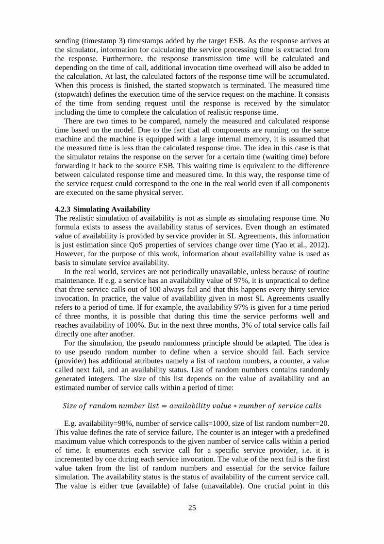
4.1.2 Availability Availability is a runtime quality of service parameter. It is usually defined by the percentage of service operation time. In this work, service availability is simply represented as true or false, no percentage will be calculated. The service is considered available as long as it replies to a request regardless of its waiting time. However the waiting time is limited by timeout of service user. Connection timeout is diverse for

21

each system. It depends on the requirement of the users of the maximum time a user is able to or willing to wait until a service responds. If the timeout is exceeded, service is assumed to be not available. Moreover it happens that a service responds an error message, meaning its HTTP response code is between 4XX and 5XX (Leach et al., n.d). In this case, service is also interpreted as unavailable.

4.1.3 Throughput This parameter gives an answer of the question of the number of users or requests a service can process within a period of time. Throughput can be a performance indicator of the service provider and its ability to process jobs concurrently (Lee, 2005). In this working context, throughput describes a statistic about the web service usage within the framework over the given period of time.

4.1.4 Reliability Reliability, also successful execution rate, can be seen as both functional and non-functional property of services. Reliability indicates the correctness of the service responses within a specified time frame (Zeng et al., 2003). On the one hand side, correct implies that the information delivered by the service provider is accurate and matched or suited to the desired request (functional requirements). An example in a real life situation is that google search engine gives proper results based on the search query. On the other hand side, correct also means that a service is delivered successfully within a maximum time defined in a service contract (SLA) or Web service description (Zeng et al., 2003); this term indicates a NF requirement. The correctness of the delivered information is difficult to measure and is not part of this work. The second, NF understanding of reliability is more suitable in the context of this work.

For this work, reliability is proposed as a comparison of target and actual performance, i.e. the promised NF properties of services defined in the SL Agreements are compared to the real measured performance of services (SL Achievement). When for example it is written in SL Agreements that the service is unavailable for less than one hour in a year, service calls will be monitored over the whole year and then analysed, whether service unavailability in reality is less than one hour.

Service providers compete on a service market with each other to acquire as many consumers as possible and grab a big market share. Therefore they need to offer a good quality impression of their service to potential consumers. All these characteristics can be found in the SL Agreement.

Likewise service intermediaries “need to specify their own SLAs while depending on the correctness of the specifications provided by their sub-services. [...,] deviations of actual non-functional characteristics and those specified in SLAs may propagate and spread even unintendedly and without control of the providers” (Kirchner et al., 2011). SL Achievement as proposed by Kirchner et al., 2011 on the other hand provides information about the real measured NF properties from the service consumers’ point of view. In this way, service consumers can analyse whether the service provider stands by its commitment and hence is trustworthy. The practical implementation to compare these two components is not part of this work.

4.2 Implementation concept Currently, the existing framework environment scenarios are running on the same physical machine, which is an isolated local host environment. Under this condition services can perform perfectly since there are no fundamental interruptions compromising their efficiency in executing tasks. This circumstance does not actually exist in the real world. To be able to generate reliable data which represent a genuine

22

world, simulation techniques should provide a way to bring real issues to the existing laboratory environment.

4.2.1 Interception of the Simulator It is conceived by the framework that all service calls first pass the integration platform which then forwards these requests to the right end point, either to another the integration platform within the integration environment or to an external service (Figure 4.1). Considering this, it is certainly the best approach to construct a simulator to represent the “world” or the internet between the integration platforms. The simulator can act as a gateway or proxy server4 between the integration platforms. In this way, the particular request packets going through the network, in this case through the gateway, can be manipulated.

Figure 4.1: Request Flow in SOC Framework

A proxy server (forward proxy) is a server or service which operates as a middleman between client (or consuming server) and server. It receives packets from one client, analyses and processes them, and then forwards them to the target server. As the target server responses to the request, the proxy collects the response, evaluates it anew, and sends it back to the client. (Schnabel, 2004)

Figure 4.2: Web Proxy Server (Schnabel, 2004)

For the purpose of this work, the to be developed simulator should adapt the concept of the proxy server. In this context, the simulator will receive packets from one integration platform, evaluate or manipulate them, and pass them to the target integration platform. As a response is sent from the target integration platform, it goes through the simulator again and will be forwarded to the requestor (see Figure 4.3).

4 Even though there are differences between gateway and proxy regarding their functionalities in real, these two terms are used synonymously in this work.

23

In the next section, the concept about how to simulate the selected NF properties will be presented.

4.2.2 Simulating Response Time

Figure 4.3: Request passing the simulator

As mentioned in Chapter 4.1.1, there are several factors affecting a service’s response time, such as transmission time, propagation delay, processing time, segmentation overhead, and invocation time overhead. Some of these parameters like transmission time and propagation delay can easily be calculated based on the given formulas. Some others need to be measured at runtime or have a complex calculation process.

In simulating response time, there are four principal events that need to be considered during the whole execution process. They are (1) “request sent”, (2) “request received”, (3) “response sent”, and (4) “response received”. To allow the simulator to generate network traffic so that integration platform shows a realistic response time, the happening of events on the network need to be monitored and controlled, especially the point of time when a response reaches the requestor (event 4). The goal is to achieve a realistic calculation of time at which a requestor receives the response. The monitoring is performed by adding timestamps to the message headers each time an event occurs. The simulator controls those events by manipulating their time of occurrence.

The idea is that before the ESB (integration platform) sends the request to the target service, it first extends the request’s message header with a timestamp and information about the consumer in terms of its unique ID in the integration environment. Here, the timestamp provides a reference about the time when a request is sent out (event 1). When a request arrives at the simulator, the simulator starts a stopwatch and forwards the request directly to the destination address (the use of the stopwatch will be explained later in this section). On the other service side, the destination ESB adds another timestamp to the request header with the time when request arrives at the destination integration platform (event 2, see Figure 4.4). The request will then be sent to the web service and is processed there.

During the service processing time, which means waiting time for the simulator, the simulator computes simultaneously the response time based on the parameters mentioned above (Chapter 4.1.1). For doing this, the simulator extracts some information needed from the received request message, like the message size and the consumer ID as well as the time of call from the message header. Additionally, there is a configuration file in XML format, which stores information about the service

24

components within the integration environment. The information encompasses existing or registered local components, service consumer context such as location and bandwidth, and service provider context such as location, availability as well as workload capacity of the service depending on the time of day. These values are specified based on realistic assumption. To define bandwidth value, speed tests are executed to get approximate value for network speed on servers, where ESB is running. For the distance calculation between service providers and consumers, an existing web service is used, which calculates the linear distance between two places based on Bing maps SDK5. The assumptions to define the workload capacity of a service are made partially based on research results from Chen et al., 2011 and Kirchner et al., 2011. Information about the service’s busy time (peak hours) as well as a time dependant penalty factor is provided in the configuration file. The penalty factor is a variable, by which the response time is increased during the given peak hours (see Chapter 4.1.1 about invocation time overhead).

Figure 4.4: Additional headers in SOAP message

The simulator can search for required details in this configuration file by using the service component’s ID as identifier. Based on the collected information, the simulator can determine request transmission time, propagation delay, and segmentation overhead (see Chapter 4.1.1 for the formula). To compute propagation delay, propagation speed needs to be declared. The assumption is that a signal propagates through cable at speed of 2.4·108 m/s (Forouzan, 2006) with Ethernet connection, which has default MTU of 1500 bytes.

When the target ESB receives a reply from a Web service and is ready to send it back to the source, timestamp information, i.e. point in time of sending the response, is added to the response message (event 3). The response is then sent back to the requestor.

Figure 4.5: Service response flow

As explained in Chapter 4.1.1 point number 3, service processing time can be computed either based on the algorithm given by the service provider or by publicly announced information. In this work, the real processing time will be measured and it is equal to the difference between request receiving (timestamp 2) and the response 5 http://www.mg2.de/map.html

25

sending (timestamp 3) timestamps added by the target ESB. As the response arrives at the simulator, information for calculating the service processing time is extracted from the response. Furthermore, the response transmission time will be calculated and depending on the time of call, additional invocation time overhead will also be added to the calculation. At last, the calculated factors of the response time will be accumulated. When this process is finished, the started stopwatch is terminated. The measured time (stopwatch) defines the execution time of the service request on the machine. It consists of the time from sending request until the response is received by the simulator including the time to complete the calculation of realistic response time.

There are two times to be compared, namely the measured and calculated response time based on the model. Due to the fact that all components are running on the same machine and the machine is equipped with a large internal memory, it is assumed that the measured time is less than the calculated response time. The idea in this case is that the simulator retains the response on the server for a certain time (waiting time) before forwarding it back to the source ESB. This waiting time is equivalent to the difference between calculated response time and measured time. In this way, the response time of the service request could correspond to the one in the real world even if all components are executed on the same physical server.

4.2.3 Simulating Availability The realistic simulation of availability is not as simple as simulating response time. No formula exists to assess the availability status of services. Even though an estimated value of availability is provided by service provider in SL Agreements, this information is just estimation since QoS properties of services change over time (Yao et al., 2012). However, for the purpose of this work, information about availability value is used as basis to simulate service availability.

In the real world, services are not periodically unavailable, unless because of routine maintenance. If e.g. a service has an availability value of 97%, it is unpractical to define that three service calls out of 100 always fail and that this happens every thirty service invocation. In practice, the value of availability given in most SL Agreements usually refers to a period of time. If for example, the availability 97% is given for a time period of three months, it is possible that during this time the service performs well and reaches availability of 100%. But in the next three months, 3% of total service calls fail directly one after another.

For the simulation, the pseudo randomness principle should be adapted. The idea is to use pseudo random number to define when a service should fail. Each service (provider) has additional attributes namely a list of random numbers, a counter, a value called next fail, and an availability status. List of random numbers contains randomly generated integers. The size of this list depends on the value of availability and an estimated number of service calls within a period of time:

�� = �� ∗ �� E.g. availability=98%, number of service calls=1000, size of list random number=20.

This value defines the rate of service failure. The counter is an integer with a predefined maximum value which corresponds to the given number of service calls within a period of time. It enumerates each service call for a specific service provider, i.e. it is incremented by one during each service invocation. The value of the next fail is the first value taken from the list of random numbers and essential for the service failure simulation. The availability status is the status of availability of the current service call. The value is either true (available) of false (unavailable). One crucial point in this

26

concept is to specify the number of service calls within a period of time. Since there are no historical data to rely on, it is difficult to make estimation. The research team concluded that it is more about the methodology than exact numbers. Availability values of different service providers differ to two decimal places, e.g. value of service A=98.75% and service B=99.25%. So the solution is to use a big number to get whole number product for the size of random number list, e.g. number of service calls=10000, availability value=98.75%, size of the list=125.

This can be shown in this simplified example for understanding: The weather service Yahoo has a list of random numbers spRandNumbList consisting of three integer values, x1=23, x2=76, x3=98; counter c which starts from value 1 for initial call, c=1; and next fail which is the first value in the list, i.e. nextFail = x1. For each service call, counter is updated and at the same time, it is compared with the value of nextFail. If the counter is equal to next fail, then the availability status is false and the service should be simulated as unavailable. In this case, the 23rd call should fail. As it occurs, x1 will be deleted from the list and nextFail is updated to be equal to x2. And the process is repeated for each service call. If the counter has reached the predefined maximum value, which is the defined total number of service calls, it is reset and starts to count again from the beginning (c=0), at the same time, spRandNumbList is restored and refilled with completely new random integers. There will also be a case, where the spRandNumbList contains two or more same integers, x1=34, x2=34, x3=89. This will be handled by skipping this same integer value and the next unequal integer will be assigned as nextFail. As an example, counter c equals to nextFail which is x1. Before nextFail is updated to the next value (x2) in spRandNumbList, it is first examined whether x2 is identical to the current first value (nextFail/x1). If it is the case, this value is removed and next value (x3) will be re-examined. This process is repeated until the next unequal value is found. This could have been fixed, but it actually resembles the fact that within a period, the service unavailability may be lower than the given value in SL Agreement, as discussed above.

27

5 Implementation This chapter describes the realisation of the simulation concepts introduced in the previous chapter. It describes how the simulator is implemented and what technologies and libraries were utilised for the development of the simulator.

The realisation of the simulator is based on Java technology, the HttpServlet is applied to develop the simulator to make it act like a proxy between the integration environments. Detailed explanation is given in the next section.

5.1 The Simulator as Java Servlet As described in the concept, the simulator should act as a Web proxy. The proxy is implemented using the Java Servlet technology. Servlets can be defined as Java programs running on a server (Ullenboom, 2006), which are processed in a so called servlet container, also known as servlet engine. Servlets are platform independent due to the nature of Java (Mordani, 2009). According to the Oracle documentation, “a servlet is a Java programming language class used to extend the capabilities of servers that host applications accessed by means of a request-response programming model” (The Java EE 6 Tutorial, 2013).

The servlet container takes an important role in a servlet-based processing environment. It is responsible for the management of all available servlets. “It is part of Web- and application server, provides network services, decodes MIME-based requests, and formats MIME-based responses” (Mordani, 2009). If a Web server receives requests from a client, it redirects them to a servlet container which then forwards the requests to the corresponding servlet instance (Ullenboom, 2006). A container may modify requests and responses before forwarding them to the servlet or back to the Web server and also give response without first contacting the servlet (Mordani, 2009).

Based on Mordani (2009), all servlets implement the servlet interface which is an abstraction of the Java servlet API. There are two classes that implement a servlet interface: GenericServlet and HttpServlet. Developers commonly extend the HttpServlet class to implement their servlets. The servlet interface defines lifecycle methods (The Java EE 6 Tutorial, 2013) for servlets. The servlet lifecycle encompasses the loading, instantiation and initialisation (init()), request handling (service(), doGet(), doPost()), and termination (destroy()) process of a servlet instance. These procedures are controlled by the servlet container. Once a container receives a request from a Web server, following steps are performed by the container:

1. Loading, instantiating the servlet class, and initialising a servlet object If no servlet instance exists (The Java EE 6 Tutorial, 2013), the container initialises a servlet object by calling the init method. There is no specific moment when the loading, instantiating, and initialising process should be executed. This can be done either when the container/server is started or at the first time the servlet is requested before it can handle a service request. Initialisation is useful for e.g. read persistent configuration data, establish a network and database connection or perform a one-time activity (Mordani, 2009).

2. Handling request The request is processed by calling the service method provided by a basic servlet interface. The HttpServlet provides additional methods for handling HTTP specific requests. There are a number of them, but the most common used are doGet() for handling GET requests and doPost() for handling POST requests (Mordani, 2009). Developers may override these methods and define their particular approach to handle requests and responses. This service methods (doGet(), doPost(), service()) are invoked for each request submitted to a servlet

28

-Dhttp.proxyHost=<host-address> -Dhttp.proxyPort=<port>

instance (Mordani, 2009) and processed in an individual thread (Ullenboom, 2006). A new thread is created for each request to a servlet and threads are processed simultaneously, i.e. the concurrent execution of service methods (Mordani, 2009).

3. Ending service If a servlet instance is not needed anymore, the servlet container calls the destroy method. This induces that acquired resources are released and allows the servlet to store any unsaved information. In case that a server, on which the servlet is running, is unexpectedly shut down or crashes, the destroy method will not be called. This means that all unsaved states will be lost. (Hunter, 1998)

The servlet application in this work extends the HttpServlet and is deployed on a JBoss application server. The integration platform is configured to use the servlet as a proxy so that all requests and responses will automatically pass through the simulator. The configuration is made by complementing the ESB run configuration file with a proxy setting option for JVM.

Simulator initialisation. During the initialisation process some activities are executed that consume a high amount of resources. The configuration XML file containing information about the environment is parsed and the content is stored in static Java objects and made available for later use in request handling. A large number of random numbers are generated and stored in an array list called randNumbList for the purpose of simulating availability. Along with those operations, an object of ScheduledExecutorService from Java’s concurrent utility class is initialised to run an asynchronous process to generate new random numbers. The ScheduledExecutorService is an interface that extends ExecutorService to run commands either periodically or after a given delay (ScheduledExecutorService, n.d). ExecutorService (Executor, n.d) is an abstraction of classes that execute Runnable (Runnable, n.d) tasks and is able to produce asynchronous tasks or computation. The intention of this asynchronous process is to monitor the quantity of random integers in the randNumbList. If it falls below the defined minimum numbers, new random integers should be generated to fill the randNumbList again. The asynchronous process runs simultaneously while the servlet is running in a different thread. Request handling. The simulator application is specified to handle HTTP-based requests and therefore overrides doGet() and doPost() methods. The procedures of handling both GET and POST requests are in this case the same. If the servlet receives a request, it processes the request by extracting the information needed for the redirection. This is the main part of the simulator. In this section the thoughts introduced in Chapter 4.2 are implemented, i.e. the calculation of response time compared with measured time and monitoring of counter and next fail value of availability. A detailed explanation of this behaviour is described in the next sections. End of Service. When the servlet needs to be removed, the destroy method resets all created objects, such as the Java objects consisting of framework environment components. It also clears the randNumbList and shuts down the submitted task of the ScheduledExecutorService object.

29

5.2 Simulating Response Time The implementation of the response time simulation is realised in the doPost method. As explained in Chapter 4.2.2, as a servlet receives requests, it redirects the requests immediately to the destination. This process is performed in a thread created by the servlet object. For the calculation of the response time based on formulas given in Chapter 4.1.1, a new thread is constructed to achieve asynchronous task accomplishment. The execution of this asynchronous process is done by the ExecutorService interface. This is initialised by creating an Executor object with the capability to “create a thread pool and generate new threads as needed” (Executors, n.d).

In this thread, request transmission time, latency, and segmentation overhead are calculated, moreover the invocation overhead based on the call time will also be determined. For the calculation, the servlet needs to obtain some information from the request itself, e.g. message size or service consumer ID. Other service consumer or provider specific information is stored in an XML-based configuration file. The servlet does not need to parse the file every time it looks up for references, because during the servlet initialisation process, they are already stored as static Java objects which are available for use during the whole servlet lifetime. This circumstance simplifies and accelerates access to the required data. The obtained data are bandwidth of service consumer, location of service consumer and provider, distance between service consumer and called service, and also peak hours of service advising about time of day, at which service utilisation rate is higher than normal or average value (see Chapter 4.1.1 about invocation time overhead).

When the submitted request has been processed, the simulator/proxy servlet receives the response and continues computing the missing parameters (response transmission time, processing time, etc.) for the response time calculation, which can only be completed with additional information within the response. The transmission time is calculated, but this time for the response message. The data to identify the service response time can be gathered by extracting information from the response message header; these are timestamps for request arrival and response sending events as explained in Chapter 4.2.2.

Once the parallel thread finishes the calculation of the respective parameters, results are delivered and summed up with transmission and processing time. Afterwards, the determination process of response time is considered as completed. The process, from sending out the request to the target service until finalising the calculation of the response time, is monitored in term of its timing. Apache Commons provide libraries to easily work with timing. The StopWatch class is utilised for this tracking purpose. It can easily be started, suspended, resumed, and stopped at any time.

At the moment when the stopwatch is terminated and the response time calculation is finished, the comparison between measured and calculated time can take place. The difference between these two values is then calculated and used as basis for the servlet to schedule, when the response is to be forwarded.

30

Figure 5.1: Sequence diagram of response time simulation

5.3 Simulating Availability The main components for the simulation of availability are lists of generated random numbers. There are two kinds of random number lists. One contains a great number of random integers and serves as a stock, from which each service provider receives random numbers for its availability. Also there is a list for each service provider that provides the indexes of those requests that should fail. The stock list of random numbers, randNumbList, is generated already during the initialisation process of the servlet object. Generating random numbers in Java demands quite a large amount of resources. This is done in advance to reduce potential overhead at runtime for the generation of random numbers. Instead, the service provider list, spRandNumbList, in the service provider objects are filled with pre-generated random numbers from the randNumbList at runtime.

During the servlet initialisation process, a large amount of random numbers are generated, stored as an array, and made available during the whole servlet lifetime. While parsing information from an XML configuration file to be stored as Java objects, each service provider object is assigned a spRandNumbList. The size of the list depends on the availability value of the corresponding service provider and a predefined number of service calls (as explained in Chapter 4.2.3). The spRandNumbList is filled by taking out a defined quantity of random integers from the randNumbList. If an integer in the randNumbList is assigned, it is then immediately removed from the list. By the time a servlet receives its first request, both lists are prepared and ready to use.

As described in Chapter 4.2.3, the service provider objects have specific attributes for the availability simulation purpose; spRandNumbList, counter c, value of next fail nextFail which is equal to the first integer in the spRandNumbList, and availability status as Boolean. If a request arrives at the servlet, in parallel with the calculation process of response time, the value of counter c is increased by one and compared with nextFail. If both values are equal, the availability status of the particular service call is false, means unavailable. In this case, nextFail is updated straight away to adopt the next integer value in the spRandNumbList and the old value is removed from the list.

Java provides the possibility to run multithreading processes within its application, i.e. different processes are executed in different threads. If a servlet receives a request, a

31

new thread is created to handle this request, i.e. concurrent processing of requests in doGet() or doPost(). To avoid concurrent access of objects in a servlet class, they need to be made thread-safe. Thread-safety means that “objects should be used only within the scope of the doGet() or doPost()” (Mordani, 2009: 28). In this simulation scenario, the service provider object accessed to monitor the availability status is not thread-safe. To avoid concurrent access that could cause failure in simulating the availability status, access to this object, especially the counter c and the nextFail attributes, is locked while these are being operated by a thread. This implies that other threads which need to access this object must wait until the other thread finishes working with the object. Java provides the synchronized method that undertakes this task. In this case, the getter method for counter and nextFail is synchronised to make them thread-safe.

Simultaneously to all the activities, another task for ExecutorService is submitted. This is applied to review the state of the counter value. The given availability value is valid only within a specific number of service calls, maxNumSC. The counter is an attribute which in a way monitors this value. When the counter reaches the maxNumSC, it should be reset to enumerate from 1 again. Furthermore, spRandNumbList is cleared for the case that the list is not empty yet, and new random numbers are taken from the general randNumbList. This process is performed in parallel, so that other processes of calculating the response time and controlling availability status do not get disturbed.

32

6 Experiment and Evaluation This section describes a validation approach for the developed simulator. First, test scenarios are introduced and then the result will be presented.

6.1 Test Scenario To test the implemented solution, the service calls within the simulator and those in the real world are compared with each other. This validation is applicable especially for validating the suggested response time model in Chapter 4.1.1. Four random Web services from four different continents are selected. These are:

1. The weather service, myweather, located in Glasgow, United Kingdom 2. The weather service, websky, located in Seoul, Korea 3. A web service providing information about team players of Australian Football

League located in Dandenong, Victoria, Australia 4. A post code service located in Washington, D.C., USA

Clients are developed to automatically call each service every three minutes, because

there is a restriction of 500 calls per day for the free Web service API. The service calls are executed from two virtual servers, one in Karlsruhe, Germany, and the other one in Kalmar, Sweden.

Just like the real service setup, the framework environment is configured in a similar way to reality. Four locally deployed services are set to be located in four different countries compliant with those of the chosen real services. Also, service consumers in the environment are configured to correspond to the location of the clients of real service calls.

Clients within the simulation invoke services every three minutes. This is the same sequence as in the real evaluation setup with real services. Response time of these service calls is monitored and the results are recorded. Both invocation results should then be compared and appraised.

6.2 Evaluation The following graphics show representatively the results of the simulator validation. They indicate the comparison between the service response time of real service calls and those within the simulation.

Figure 6.1: Response time comparison of service calls from Karlsruhe to United Kingdom

0

500

1000

1500

2000

1

37

73

109

145

181

217

253

289

325

361

397

433

469

505

541

577

613

649

685

721

757

Re

spo

ne

s T

ime

(m

s)

Number of Service Calls

Karlsruhe - United Kingdom

Real

Simulated

33

Figure 6.2: Response time comparison of service calls from Kalmar to United Kingdom

Figure 6.3: Response time comparison of service calls from Karlsruhe to Korea

Figure 6.4: Response time comparison of service calls from Kalmar to Korea

As noticeable from Figure 6.1 - Figure 6.4, there is a significant variance of response time between the simulated and the real service calls. Due to the fact that the creation of model calculating response time is based on assumption and not absolutely considering

0

500

1000

1500

2000

1

36

71

106

141

176

211

246

281

316

351

386

421

456

491

526

561

596

631

666

701

736

Re

spo

nse

Tim

e (

ms)


Kalmar - United Kingdom

Real

Simulated

0

5000

10000

15000

20000

25000

30000

1

37

73

109

145

181

217

253

289

325

361

397

433

469

505

541

577

613

649

685

721

757

Re

spo

nse

Tim

e (

ms)


Karlsruhe - Korea

Real

Simulated

0

5000

10000

15000

20000

25000

30000

1

35

69

103

137

171

205

239

273

307

341

375

409

443

477

511

545

579

613

647

681

715

Re

spo

nse

Tim

e (

ms)


Kalmar - Korea

Real

Simulated

34

all factors existing in the real world, differences between the results were expected. The huge deviations though are assumed to occur because of following reasons:

- Unique service instance. The validation was carried out only against one service from each continent. And services behave differently in different networks. The market of services is huge and there are some unpredictable effects in the real world that cannot be controlled and thus are very difficult to simulate. It is assumed that the developed model could conform to some kind of ordinary services. To achieve more exact results, validation should be conducted with a larger number of Web services providing similar functionality.

- Service complexity. The service calls within the simulation invoke some simple self-implemented Web services with a literally small processing time. Service calls in the real world validation scenario invoke some randomly selected Web services of different complexity. The selection process of those real Web services was focused on the services’ location. The variety of complexity of these services was not considered. The higher processing time of real world services due to the individual complexity might be a reason for the longer response time (see further tests of ping calls, Figure 6.6 and Figure 6.7).

- Server capacity. Depending on service complexity, the performance of the server on which the Web services are deployed is also one factor that could influence the service processing time. Usually, not only a single service is running on a Web server. Therefore services must share resources with each other. Depending on the service complexity, performance or behaviour of the servers (e.g. number of simultaneous users or current use of resources), service requests might be processed rapidly or slower.

- Routing mechanism. In the Internet era, a large number of computers (nodes) are globally connected with each other in some way. “Connectivity between two nodes does not necessarily imply a direct physical connection between them, indirect connectivity might be achieved among a set of cooperating nodes” (Peterson and Davie, 2011). There are various ways to connect from one node to the other. As to connect from the clients in Karlsruhe and Kalmar to Web services in the respective locations, different paths can be chosen to pass through. The path to the target node should usually be efficient (e.g. as short as possible) to reduce the travelling time. There is still a possibility that the connection is routed to a circuitous way, which extends the travelling time. As seen in Figure 6.5, one can choose path number 1 to travel from point A to B, which is the direct way. However, there are other alternatives like going through path number 2, 7, and 8 (i.e. A � F � D � B). This kind of routing mechanism or path is generally not taken into consideration in the simulation model, only the direct distance between source and destination node was used to calculate the travelling (or transmission) time.

Apart from the distance, the packets going through the network must pass each of the nodes (router) along the routing path. Before forwarding the packets, router needs to look up for forwarding information such as destination address or suitable output ports in a so called forwarding or routing table (Peterson and Davie, 2011). This lookup process occurs on each router and causes also additional delay.

35

Figure 6.5: Network as a graph (based on Peterson and Davie, 2011)

Additionally, ping tests were conducted to estimate the processing time and network transfer time of real Web services.

Figure 6.6: Comparison between time for ping calls and simulation from Kalmar to Korea

In the case of the service from Korea, real service calls have an average response time of over 14000ms. For comparison, the ping to the service provider’s website domain has an average value of 331ms. This shows that the response time presented on Figure 6.4 is composed mostly of processing time. Still there are differences between the ping time and the time from the simulation. It can be argued, that routing paths from Kalmar to Korea is longer than only the beeline (linear/direct distance) which is used by the model. The results of the pings and the simulation for the service in the United Kingdom are nearly similar (Figure 6.7). This shows that the calculated service response time within the simulation is almost equal to network transfer time of real service. In spite of all that, on the Figure 6.8, it is to be noticed that the results of the calculated response time are varying apparently relative to the location of the Web services. It shows that the simulator can manipulate the NF properties of services depending on the context of service components.

0

100

200

300

400

1

36

71

106

141

176

211

246

281

316

351

386

421

456

491

526

561

596

631

666

701

736

771

806

841

Tim

e (

ms)


Kalmar - Korea

ping

simulation

36

Figure 6.7: Comparison between time of ping calls and simulation from Kalmar to United Kingdom

Figure 6.8: Response time comparison of service calls within simulation

After carrying out some investigations it was found, that in some cases, where the distance between source integration platform and destination integration platform is short, e.g. when both, service consumer and provider, reside in the same country, the simulated response time is not compliant with the time, the simulation model would predict (see Chapter 4.1.1). The reason for this is that calculating desired response time in the simulator in such cases takes longer than the time, the model predicts as response time. Consequently, the time recorded by local components is the calculation time instead of the actual response time compliant to the model. This unintentional error is particularly noticeable because the self-implemented Web services within the simulation environment are very simple services which do not perform any calculations. On that account, services respond rapidly and the processing time is far quicker than the time to calculate the desired response time. This would probably not occur, if the simulation flow is done using reasonable complex services. Possible optimisations for this issue are described in Chapter 7.2 Future Work.

Validation was also executed to examine the implementation to simulate service unavailability. Each service provider has an availability value, which was defined to apply for 10000 service calls. Services located in Australia and the USA were configured with an availability value of 98.25%. These values mean that, based on the described concept in Chapter 4.2.3 and 5.3, services have a sorted list of random

0

50

100

150

1

36

71

106

141

176

211

246

281

316

351

386

421

456

491

526

561

596

631

666

701

736

771

806

841

Tim

e (

ms)



ping

simulation

0

50

100

150

200

1

49

97

145

193

241

289

337

385

433

481

529

577

625

673

721

769

817

865

913

961

Re

spo

nse

Tim

e (

ms)


Simulated Calls from Karlsruhe

USA

Australia

Korea

United Kingdom

37

numbers containing 175 random integers, i.e. the maximum number of service unavailability is 175 times within 10000 service calls.

Figure 6.9: Comparison of simulated service availability with the same availability value

As seen in the evaluation results above, the simulation system is able to simulate NF

properties based on the given model. The simulation results (response time) are however not similar to the real world due to some reasons also described above. Nevertheless, different simulation results due to the variation of input parameters can still be achieved. Because of time constraint, a graphical user interface for configuration purpose could not be developed. The simulation system is certainly provided with a simple configuration file containing information about the laboratory framework environment. Using this file, users of the simulation system can also change the input parameters based on their requirement for the simulation process. Further development suggestion will be presented in Chapter 7.2 about the future work.

9828 9825

172 175

0

1000

2000

3000

4000

5000

6000

7000

8000

9000

10000

Australia

(98.25%)

USA

(98.25%)

Nu

mb

er

of

Se

rvic

e C

all

s

Service Location

Simulated Service Availability

unavailable

available

38

7 Conclusion This final chapter gives an overall summary of this work as well as an outlook about further improvement and development for the future.

7.1 Summary This thesis describes the concept and implementation of a simulation environment. The simulation environment is used as an instrument to verify the SOC framework. In this framework, the key component, called central component or service broker, analyses and evaluates data about service calls within the integration environments (see Chapter 1.3.3). This process aims to compare service instances based on their NF properties and to help service consumers in selecting the best-fit service provider on the basis of consumer context and utility value. The analysed data come from the local component which monitors and measures NF attributes of services during invocation.

Using the simulation, NF properties like availability and response time can be manipulated. Since all framework components (central component, integration platform, and service components) are running on the same machine (see Chapter 3.1) and services perform without any influences from outside networks, the measured data regarding service calls are not considered realistic for the evaluation purpose. The developed simulator can calculate service response time based on a simplified model (see Chapter 4.1.1) and simulate this effect. For example, a service call from Karlsruhe, Germany, to Sydney, Australia, should have a higher response time than a call to London, United Kingdom. For the calculation, a configuration file is available containing information about the location of the service providers and consumers, bandwidth of service consumers, availability of service providers, etc. Furthermore, the simulator can also simulate service availability. Each service provider has a counter, which enumerates every service call, and a list of random numbers with a defined size. The size is determined based on the availability value in configuration file and the total number of calls, which the availability value is applied to (see Chapter 4.2.3).

With the simulator, local components can now capture sample data which complies with reality conceptually. As the validation has shown, even though the values of simulated response time are not identical to those in the real world, the developed model indicates different results of service calls to various locations. The model can thus be optimised to draw closer to reality. Nevertheless the crucial matter for the learning process by the central component, which is assessing the varieties of service NF properties depending on service providers’ and consumers’ context, is covered by the operation of this simulator.

Referring to goal criteria, described in Chapter 1.4, three out of five desired characteristics of the simulation system could be fulfilled. For the development of the simulator, minor extensions are made to the existing local component. The simulator is still an independent component, which can easily be attached and detached from the framework environment (criteria 1 and 2). This condition allows simple further modification and development without affecting the existing laboratory environment. Since the simulator is built as a servlet, the integration platform can be configured to use the simulator as a proxy. As already mentioned, the simulator can simulate different NF properties determined by the model (Chapter 4.1.1 and 4.1.2) and input parameters (criterion 5). Even though the model yields different results based on the input parameters, still there is a big variance between the simulation results and real service call results (criterion 3). These could be fixed by optimizing the input parameters for the defined model (see next chapter). Due to lack of time, no graphical user interface was built for the configuration of simulation’s input parameters (criterion 4).

39

7.2 Future Work The desired simulator was implemented successfully, yet some missing functionalities and improvement potentials were also identified.

- Simulator optimisation In order to achieve response time values closer to reality, the developed model needs to be enhanced to consider more advance factors in the real world into the implementation. One parameter for response time calculation was propagation delay. This value is computed by dividing distance between source and destination by propagation speed. In the current simulation implementation, the distance is a straight line between two locations and the propagation speed is equal to 2.4·108 m/s (propagation speed of signal through cable). The calculation of these values is not technically precise. As explained in the validation result (Chapter 6.2), routing is one influencing factor in the Internet world. Distance and paths to transmit requests from service consumer to designated destination are not always the same, because there are a big number of alternative links. Besides, the medium to transfer signal from source to destination is not the same along the whole paths. The formula can be expanded by dividing the route into small sections as well as making use of different propagation speeds in different sections.

During the simulation, there are cases, in which simulation results are not consistent with the model, i.e. simulator needs longer time to calculate and forward the response to consumer than the response time determined by the model. After the simulator receives the response back from the target service, it has to read the message to obtain information about the service processing time. This process of extracting the response is assumed to be time-consuming and the cause of delay in the simulation. Further evaluation is required to discover other possible reasons and improve this process.

- Functional extension of the simulation At the moment, the local components capture just the two simulated NF properties, namely response time and availability. The simulation environment can be developed further to support the simulation of other network characteristics effecting the measurement of desired NF properties. Further studies are necessary to decide relevant NF properties for the selection of best-fitting service provider.

- Dashboard for configuring the simulation A nice-to-have feature to complete the simulator would be a dashboard like configuration surface. In the current implementation, the simulator is provided with a configuration file. This file contains detailed information about the framework environment needed for the simulation process, such as location of service providers or consumers, availability value, utilisation rate of service providers for specific point in time, and also bandwidth of service consumers. The configuration file is available in XML format. To be able to set different scenarios for the simulation, users need to directly modify this file which could be problematic for users without understanding of XML. The dashboard should facilitate users with a graphical interface to easily change the simulation configuration without direct modification to the file and hence create various simulation scenarios.

40

References Altmann, E., Jiménez, T., 2003. NS Simulator for Beginners, lecture notes, 2003-2004. Universidad de Los Andes, Merida, Venezuela and ESSI, Sophia-Antipolis, France. Banks, J., Carson II, J.S., Nelson, B.L., Nicol, D.M., 2005. Discrete-event system simulation, 4th ed. Pearson Prentice Hall, Upper Saddle River, New Jersey.

Banks, J., Carson II, J.S., Nelson, B.L., Nicol, D.M., 2010. Discrete-event system simulation, 5th ed. Pearson Prentice Hall, Upper Saddle River, New Jersey.

Bichier, M., Lin, K.-J., 2006. Service-oriented computing. Computer 39, pp. 99–101.

Buss, A., 2002. Component based Simulation Modelling with Simkit. Presented at the Proceedings of the 2002 Winter Simulation Conference, San Diego, CA, USA, pp. 243–249 vol.1.

Carson, M., Santay, D., 2003. NIST Net: a Linux-based network emulation tool. ACM SIGCOMM Computer Communication Review 33, 111–126.

Chandrasekaran, S., Silver, G., Miller, J.A., Cardoso, J., Sheth, A.P., 2002. Web service technologies and their synergy with simulation. Presented at the Proceedings of the 2002 Winter Simulation Conference, San Diego, CA, USA, pp. 606 – 615 vol.1.

Chang, X., 1999. Network simulations with OPNET. Presented at the Proceedings of the 1999 Winter Simulation Conference Proceedings, Phoenix, AZ, USA, vol. 1, pp. 307 –314.

Chen, L., Yang, J., Zhang, L., 2011. Time Based QoS Modeling and Prediction for Web Services, in: Kappel, G., Maamar, Z., Motahari-Nezhad, H.R. (Eds.), Service-Oriented Computing, Lecture Notes in Computer Science. Springer Berlin Heidelberg, pp. 532–540. Clemmensen, D., Zhang, J., Li, N., 2004. Graphical Editor. J-Sim Official. Available from https://sites.google.com/site/jsimofficial/geditor----graphical-editor (accessed 5.4.13).

Comer, D., 2009. Computer networks and internets, 5th ed. Prentice Hall, Upper Saddle River, New Jersey.

Component Architecture, 2005. J-Sim Official. Available from https://sites.google.com/site/jsimofficial/component-arch (accessed 5.4.13).

Dawson, T., 2000. NISTNet: Emulating Networks on Your Own LAN. O’Reilly Media. Available from http://www.linuxdevcenter.com/pub/a/linux/2000/06/22/LinuxAdmin.html?page=1 (accessed 5.5.13).

Emmel, J., 2011. Entwurf und prototypische Implementierung einer Architektur zur optimierenden Service-Komposition (Bachelor Thesis). Hochschule Karlsruhe für Technik und Wirtschaft, Karlsruhe. Executor (Java Platform SE 6), n.d. Available from http://docs.oracle.com/javase/6/docs/api/java/util/concurrent/Executor.html (accessed 9.21.13).

Executors (Java Platform SE 6), n.d. Available from http://docs.oracle.com/javase/6/docs/api/java/util/concurrent/Executors.html (accessed 9.21.13).

Forouzan, B.A., 2006. Data Communications Networking, 4th ed. Mcgraw-Hill Higher Education, New York.

Georgakopoulos, D., Papazoglou, M.P. (Eds.), 2008. Service-Oriented Computing. The MIT Press, Cambridge, Massachusetts.

Göbel, J., 2006. Development of a Model for Telecommunication Network Simulation with Bandwidth Trading and Link Failure Recovery (Diploma Thesis). University of Hamburg, Hamburg.

Goldberg, R.P., 1974. Survey of virtual machine research. Computer, vol. 7, pp. 34–45. Gupta, D., Cherkasova, L., Gardner, R., Vahdat, A., 2006. Enforcing performance isolation across virtual machines in Xen. Presented at the Proceedings of the ACM/IFIP/USENIX 2006 International Middleware Conference. Springer-Verlag New York, Inc., New York, USA, pp. 342–362. Hartmann, S., 2005. The World as a Process: Simulations in the Natural and Social Sciences.

41

Available from http://philsci-archive.pitt.edu/2412/1/Simulations.pdf (accessed 2.13.13).

Hasan, M.S., Harding, C., Yu, H., Griffiths, A., 2005. Modeling delay and packet drop in Networked Control Systems using network simulator NS2. International Journal of Automation and Computing, vol. 2, pp. 187–194. Huang, W., Liu, J., Abali, B., Panda, D.K., 2006. A case for high performance computing with virtual machines. Presented at the Proceedings of the 20th Annual International Conference on Supercomputing. ACM, New York, USA, pp. 125–134.

Hunter, J., 1998. Java Servlet Programming, 1st ed. O’Reilly Media, Sebastopol, California.

Issariyakul, T., Hossain, E., 2009. Introduction to Network Simulator NS2. Springer Science+Business Media, LLC, New York.

J-Sim Official, n.d. Available from https://sites.google.com/site/jsimofficial/ (accessed 7.30.13).

Keshav, S., 1997. REAL 5.0 Overview. Available from http://www.cs.cornell.edu/skeshav/real/overview.html (accessed 5.4.13)

Kirchner, J., Lowe, W., Andersson, J., Heberle, A., 2011. Service Level Achievements – Distributed Knowledge for Optimal Service Selection. Presented at the 9th IEEE European Conference on Web Services (ECOWS), Lugano, Switzerland, pp. 125–132. Köksal, M.M., 2008. A Survey of Network Simulators Supporting Wireless Networks. Graduate School of Natural and Applied Sciences, Middle East Technical University, Ankara, Turkey. Krafzig, D., Banke, K., Slama, D., 2005. Enterprise SOA: Service-Oriented Architecture Best Practices. Prentice Hall Professional, Upper Saddle River, New Jersey.

Law, A.M., 2000. Simulation Modeling and Analysis, 3rd ed. McGraw-Hill, New York. Law, A.M., 2007. Simulation Modeling and Analysis, 4th ed. McGraw-Hill, New York.

Leach, P.J., Berners-Lee, T., Mogul, J.C., Masinter, L., Fielding, R.T., Gettys, J., n.d. Hypertext Transfer Protocol -- HTTP/1.1. Available from http://tools.ietf.org/html/rfc2616#section-10 (accessed 7.30.13).

Lee, A.K., 2005. Comparison between WSQM & QoS FE Qualities. Available from https://www.oasisopen.org/committees/document.php?document_id=15444&wg_abbrev=fwsi-fesc (accessed 8.12.13)

Liu, W., Du, Z., Chen, Y., Chai, X., Wang, X., 2010. On an Automatic Simulation Environment Customizing Services for Cloud Simulation Center. Presented at the 5th IEEE International Symposium on Service Oriented System Engineering (SOSE), pp. 214 –221.

Malowidzki, M., 2004. Network Simulators: A Developer’s Perspective. Presented at the 2004 International Symposium on Performance Evaluation of Computer and Telecommunication Systems SPECTS’04, San Jose, USA, pp. 1–9. Miller, J.A., Cardoso, J., Silver, G., 2002. Using simulation to facilitate effective workflow adaptation. Presented at the Proceedings of the 35th Annual Simulation Symposium, San Dieago, CA, USA, pp. 177 – 181.

Mondesir, C., Dan, C., Koussouris, S., Texier, L., 2007. JBoss Application Server. JBoss. Docs. Available from http://docs.jboss.org/jbossas/docs/Getting_Started_Guide/4/html/index.html (accessed 3.9.13). Mordani, R., 2009. Java Servlet Specification. Sun Microsystem, Inc., California. Available from http://download.oracle.com/otndocs/jcp/servlet-3.0-fr-oth-JSpec/ (accessed 6.23.13).

Nattrass, S., 2005. Novell Cool Solutions: An Introduction to JBoss. Available from http://www.novell.com/coolsolutions/feature/14912.html#4.0 (accessed 3.9.13).

NIST Net Home Page, n.d. Available from http://www-x.antd.nist.gov/nistnet/ (accessed 7.30.13).

ns-2, 2011. Available from http://nsnam.isi.edu/nsnam (accessed 7.30.13).

OMNeT++, n.d. OMNeT++ Network Simulation Framework. Available from http://omnetpp.org (accessed 7.30.13).

Page, B., Kreutzer, W., 2005. The Java Simulation Handbook: Simulating Discrete Event Systems with UML and Java. Shaker Verlag, Aachen.

42

Paiko, M., 2012. VMware Workstation 8 as an Alternative to VMware Serve. VMware Workstation Zealot. Available from http://blogs.vmware.com/workstation/2012/02/vmware-workstation-8-as-an-alternative-to-vmware-server.html (accessed 2.24.13).

Papazoglou, M., 2008. Web Services: Principles and Technology. Pearson Education, Essex, England.

Papazoglou, M.P., 2003. Service-oriented computing: concepts, characteristics and directions. Presented at the Proceedings of the 4th International Conference on Web Information Systems Engineering (WISE 2003), Rome, Italy, pp. 3 – 12. Peterson, L.L., Davie, B.S., 2011. Computer Networks, Fifth Edition: A Systems Approach, 5th ed. Morgan Kaufmann, Burlington, Massachusetts.

Popek, G.J., Goldberg, R.P., 1974. Formal requirements for virtualizable third generation architectures. Communications of the ACM, vol. 17, pp. 412–421.

Ross, E., 2004. Configuring Multiple JBoss Instances On One Machine JBoss Community. Available from https://community.jboss.org/wiki/ConfiguringMultipleJBossInstancesOnOneMachine (accessed 3.9.13).

Runnable (Java Platform SE 6), n.d. Available from http://docs.oracle.com/javase/6/docs/api/java/lang/Runnable.html. (accessed 9.21.13).

ScheduledExecutorService (Java Platform SE 6), n.d. Available from http://docs.oracle.com/javase/6/docs/api/java/util/concurrent/ScheduledExecutorService.html (accessed 9.21.13). Schnabel, P., 2004. Netzwerktechnik-Fibel: Grundlagen, Übertragungstechnik und Protokolle, Anwendungen und Dienste, Sicherheit, 1st ed. Books on Demand GmbH.

Shute, G, 2007. CPU Performance. Available from http://www.d.umn.edu/~cprince/courses/cs2521/arch/performance/speed.html (accessed 10.20.13)

Siraj, S., Gupta, A.K., Rinku-Badgujar, R., 2012. Network Simulation Tools Survey. International Journal of Advanced Research in Computer and Communication Engineering, vol. 1, no. 4, pp. 201-210.

The Java EE 6 Tutorial, 2013. Oracle. Available from http://docs.oracle.com/javaee/6/tutorial/doc/bnafe.html (accessed 9.21.13)..

Thorns, F., 2008. Das Virtualisierungs-Buch : [Konzepte, Techniken und Lösungen; VMware, MS, Parallels, Xen u.v.a.], 2nd ed. C & L, Computer- und Literatur-Verlag, Böblingen.

Tutorial: Working with J-Sim, 2003. J-Sim Official. Available from https://sites.google.com/site/jsimofficial/j-sim-tutorial (accessed 5.4.13).

Ullenboom, C., 2006. Java ist auch eine Insel, 5th ed. Galileo Press, Bonn.

User Manual Omnet++, n.d. Omnet++. Available from http://www.omnetpp.org/doc/omnetpp/manual/usman.html#sec115 (accessed 7.30.13).

Varga, A., 2010. OMNeT++ in a Nutshell. OMNeT++ Wiki. Available from http://www.omnetpp.org/pmwiki/index.php?n=Main.OmnetppInNutshell (accessed 5.4.13).

Varga, A., Hornig, R., 2008. An overview of the OMNeT++ simulation environment. Presented at the Proceedings of the 1st International Conference on Simulation Tools and Techniques for Communications, Networks, and Systems. ICST (Institute for Computer Sciences, Social-Informatics and Telecommunications Engineering), Brussels, Belgium, pp. 60:1–60:10.

VIX 1.12 Getting Started, n.d. VMWare. Available from http://www.vmware.com/support/developer/vix-api/vix112_reference/ (accessed 12.15.12).

VMware Support Policies, n.d. Available from http://www.vmware.com/support/policies/product-eoa.html (accessed 9.21.13), http://www.vmware.com/products/server/overview.html (accessed 12.15.12).

WANem 2.0 - Wide Area Network Emulator, 2008. Tata Consultancy Services.

Weerawarana, S., Curbera, F., Leymann, F., Storey, T., F. Ferguson, D., 2005. Web services

43

platform architecture: soap, wsdl, ws-ploicy, ws-addressing, ws-bpel, ws-reliable messaging, and more. Prentice Hall PTR, Upper Saddle River, New Jersey. Weingartner, E., vom Lehn, H., Wehrle, K., 2009. A Performance Comparison of Recent Network Simulators. Presented at the IEEE International Conference on Communications 2009, Dresden, Germany, pp. 1–5.

Yao, L., Sheng, Q.Z., Maamar, Z., 2012. Achieving High Availability of Web Services Based on A Particle Filtering Approach. International Journal of Next-Generation Computing, vol. 3, no 2. Zeng, L., Benatallah, B., Dumas, M., Kalagnanam, J., Sheng, Q.Z., 2003. Quality driven web services composition. Presented at the Proceedings of the 12th International Conference on World Wide Web. ACM, New York, USA, pp. 411–421.

44

Apendix A Detailed Validation Results Followings are comparisons of response time between real service calls and within the simulation.

0

500

1000

1500

2000

2500

3000

3500

4000

1

38

75

112

149

186

223

260

297

334

371

408

445

482

519

556

593

630

667

704

741

778

Re

spo

nse

Tim

e (

ms)


Karlsruhe - Australia

Real

Simulated

0

1000

2000

3000

4000

1

38

75

112

149

186

223

260

297

334

371

408

445

482

519

556

593

630

667

704

741

778

Re

spo

nse

Tim

e (

ms)


Karlsruhe - USA

Real

Simulated

0

5000

10000

15000

20000

25000

30000

1

37

73

109

145

181

217

253

289

325

361

397

433

469

505

541

577

613

649

685

721

757

Re

spo

nse

Tim

e (

ms)


Karlsruhe - Korea

Real

Simulated

45

0

500

1000

1500

2000

1

37

73

109

145

181

217

253

289

325

361

397

433

469

505

541

577

613

649

685

721

757

Re

spo

ne

s T

ime

(m

s)



Real

Simulated

0

500

1000

1500

2000

2500

3000

3500

4000

1

36

71

106

141

176

211

246

281

316

351

386

421

456

491

526

561

596

631

666

701

736

Re

spo

nse

Tim

e (

ms)


Kalmar - Australia

Real

Simulated

0

500

1000

1500

2000

2500

3000

3500

4000

1

35

69

103

137

171

205

239

273

307

341

375

409

443

477

511

545

579

613

647

681

715

Re

spo

nse

Tim

e (

ms)


Kalmar - USA

Real

Simulated

46

Followings are comparisons of the simulated service calls with different locations setting.

0

5000

10000

15000

20000

25000

30000

1

35

69

103

137

171

205

239

273

307

341

375

409

443

477

511

545

579

613

647

681

715

Re

spo

nse

Tim

e (

ms)


Kalmar - Korea

Real

Simulated

0

500

1000

1500

2000

1

36

71

106

141

176

211

246

281

316

351

386

421

456

491

526

561

596

631

666

701

736

Re

spo

nse

Tim

e (

ms)



Real

Simulated

0

50

100

150

200

1

40

79

118

157

196

235

274

313

352

391

430

469

508

547

586

625

664

703

742

781

Re

spo

nse

Tim

e (

ms)


Simulated Calls from Karlsruhe

USA

Australia

Korea

United Kingdom

47

Following graphics show comparison between ping calls and simulated service calls.

0

50

100

150

200

1

37

73

109

145

181

217

253

289

325

361

397

433

469

505

541

577

613

649

685

721

Re

spo

nse

Tim

e (

ms)


Simulated Calls from Kalmar

Australia

USA

Korea

United Kingdom

0

50

100

150

200

250

300

350

400

1

39

77

115

153

191

229

267

305

343

381

419

457

495

533

571

609

647

685

723

761

799

837

Tim

e (

ms)


Karlsruhe - Australia

ping

simulation

0

20

40

60

80

100

120

140

1

39

77

115

153

191

229

267

305

343

381

419

457

495

533

571

609

647

685

723

761

799

837

Tim

e (

ms)


Karlsruhe - USA

ping

simulation

48

0

50

100

150

200

250

300

350

400

1

39

77

115

153

191

229

267

305

343

381

419

457

495

533

571

609

647

685

723

761

799

837

Tim

e (

ms)


Karlsruhe - Korea

ping

simulation

0

100

200

300

400

500

1

39

77

115

153

191

229

267

305

343

381

419

457

495

533

571

609

647

685

723

761

799

837

Tim

e (

ms)



ping

simulation

0

50

100

150

200

250

300

350

400

1

39

77

115

153

191

229

267

305

343

381

419

457

495

533

571

609

647

685

723

761

799

837

Tim

e (

ms)


Kalmar - Australia

ping

simulation

49

0

20

40

60

80

100

120

140

1

39

77

115

153

191

229

267

305

343

381

419

457

495

533

571

609

647

685

723

761

799

837

Tim

e (

ms)


Kalmar - USA

ping

simulation

0

50

100

150

200

250

300

350

400

1

39

77

115

153

191

229

267

305

343

381

419

457

495

533

571

609

647

685

723

761

799

837

Tim

e (

ms)


Kalmar - Korea

ping

simulation

0

20

40

60

80

100

120

140

160

1

39

77

115

153

191

229

267

305

343

381

419

457

495

533

571

609

647

685

723

761

799

837

Tim

e (

ms)



ping

simulation

50

This graphic indicates the simulated availability of services.

9828 9825 9925 9828

172 175 75 172

0

1000

2000

3000

4000

5000

6000

7000

8000

9000

10000

Australia

(98.25%)

USA

(98.25%)

United Kingdom

(99.25%)

Korea

(98.25%)

Nu

mb

er

of

Se

rvic

e C

all

s

Service Locations (Availability Value)

Simulated Service Availability

unavailable

available

Faculty of Technology SE-391 82 Kalmar | SE-351 95 Växjö Phone +46 (0)772-28 80 00 [email protected] Lnu.se/faculty-of-technology?l=en

Date post:	22-Feb-2022
Category:	Documents
Upload:	others
View:	2 times
Download:	0 times

Simulation and Measurement of Non-Functional Properties of ...

Documents