Simulation-based Optimization, Reasoning and Control:
The eRobotics Approach Towards Intelligent Robots
L. Atorf*, M. Schluse*, J. Roßmann*
*Institute for Man-Machine Interaction, RWTH Aachen University
Ahornstr. 55, 52074 Aachen, Germany
e-mail: {atorf, schluse, rossmann}@mmi.rwth-aachen.de
Abstract
Virtual Testbeds enable simulations which are at the
same time comprehensive on system level and detailed
on component level regarding all relevant inner and outer
dependencies of complex technical systems. Virtual
Testbeds are able to accurately predict the behavior of
such systems with respect to different system states,
environmental conditions or input values. That is why
Virtual Testbeds are an ideal basis for new simula-
tion-based engineering and control approaches. They
support the engineer in making the correct decisions
during the engineering process by optimizing system
parameters. They support the system itself in the real
world to make the correct decisions to find, evaluate, and
optimize the best way to reach a goal—and they enable
to seamlessly transfer a controller developed in a 3D
simulation environment to the physical system. This is
the eRobotics approach towards intelligent robots based
on state-of-the-art 3D simulation technology.
1 Introduction
Today, simulation technology is mainly used to in-
vestigate well-defined sub-problems, resulting in a dis-
continuous use of different simulation systems during the
entire engineering process. In contrast to this,
state-of-the-art “Virtual Testbed” (VTB, see Figure 1)
concepts combine these simulation approaches to setup
comprehensive simulations on system level. They pro-
vide simulations which are at the same time detailed on
component level, comprehensive on system level, and
are able to perform in real-time. To provide an overall
picture of the developed system, VTBs do not only con-
sider the system itself (e.g. the robot, its mechanical
structure, its sensors and actuators) but also its environ-
ment (e.g. the planetary surface), the environmental
conditions (light, dust, etc.) and the data processing algo-
rithms (controllers, supervisors, image processing). The
entire system as well as the sub-components provide the
very same interfaces as their physical counterparts at
least on a semantic level. In addition to this, the virtual
and physical sub-components have the same input-out-
put-behavior. Hence VTBs can be used as virtual substi-
tutes for the development of high level controllers.
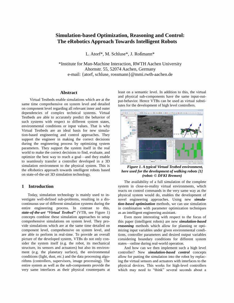
Figure 1. A typical Virtual Testbed environment,
here used for the development of walking robots [1]
(robot: © DFKI Bremen)
The availability of a full simulation of the complete
system in close-to-reality virtual environments, which
reacts on control commands in the very same way as the
physical system would do, enables the development of
novel engineering approaches. Using new simula-
tion-based optimization methods, we can use simulation
in combination with parameter optimization techniques
as an intelligent engineering assistant.
Even more interesting with respect to the focus of
this paper (intelligent robots) are new simulation-based
reasoning methods which allow for planning or opti-
mizing input variables under given environmental condi-
tions, controller parameters and desired output variables
considering boundary conditions for different system
states—online during real-world operation.
And how can we then implement such a high level
controller? New simulation-based control concepts
allow for putting the simulation into the robot by replac-
ing the virtual sensors and actuators with interfaces to the
physical devices. This works for high-level controllers
which may need to “think” several seconds about a
problem to find a solution, for intelligent sensors
providing semantic data of the environment every second
in soft real-time as well as for low-level controllers
commanding manipulators in a milliseconds interval
under hard real-time restrictions.
The result is a framework to develop and implement
intelligent robotic systems. Using “simulation inside”
they become situation aware (environment perception,
understanding and projection of semantic world models)
and are able to make decisions, plan actions and execute
these plans in real-world environments. For this, this
paper introduces a systematic and mathematic approach
to simulation-based optimization, reasoning, and con-
trol. It illustrates how to model and simulate complex
systems on system level and how this simulation can be
used to enhance engineering processes, to enable robots
to perceive their environment using intelligent sensors, to
allow robots to plan their actions using such semantic
world models, and to execute these actions as well. All
this is based on one single system/environment model
and one single data processing system implementation.
The rest of this paper is organized as follows. In
chapter 2 we introduce the basic concepts of eRobotics
and VTBs providing the conceptual and technical basis
for the rest of the paper. Chapter 3 introduces the com-
mon mathematical basis of the simulation-based optimi-
zation, reasoning and control approaches which are out-
lined in chapter 4, 5 and 6. Chapter 7 gives a short sum-
mary and an outlook on our future work in this field.
2 The basic concepts of eRobotics
The research field of eRobotics is currently an active
domain of interest for scientists working in the area of
“eSystems engineering”. The aim of eRobotics is to
provide a comprehensive software environment for a
continuous and systematic computer support during the
entire life cycle of complex technical systems. In this
way, the ever increasing complexity of current comput-
er-aided technical solutions will be kept manageable.
To do this, eRobotics provides various engineering
methods (see Figure 2), which can be used in the differ-
ent stages of a system life cycle. The methods all rely on
3D simulation technology and comprise first of all the
methods necessary for 3D visualization, 3D animation,
3D simulation and “(Projective) Virtual Reality”. New
concepts of “Semantic World Modeling” [2] provide the
methods necessary to set up models of components,
systems, environments, controllers, supervisors, etc. The
integration of data processing algorithms like image
processing or generic controllers or supervisors leads to
VTBs. Such VTBs are the basis for the simulation-based
approaches as introduced in this paper.
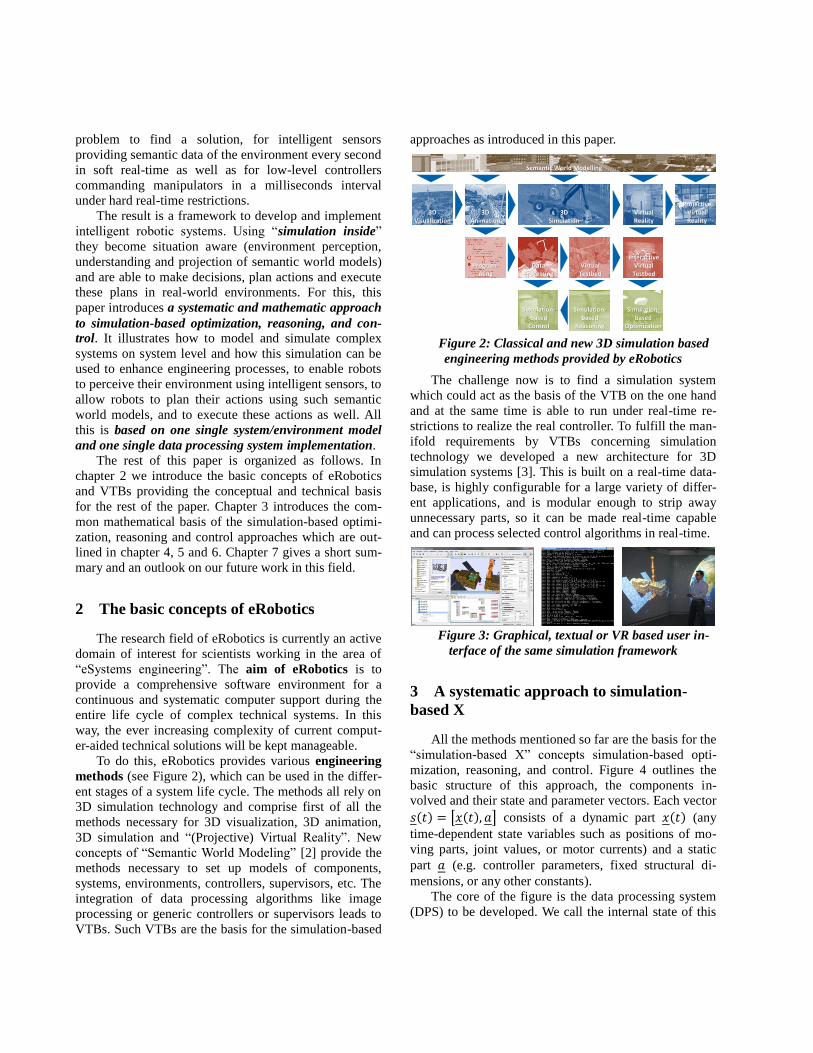
Figure 2: Classical and new 3D simulation based
engineering methods provided by eRobotics
The challenge now is to find a simulation system
which could act as the basis of the VTB on the one hand
and at the same time is able to run under real-time re-
strictions to realize the real controller. To fulfill the man-
ifold requirements by VTBs concerning simulation
technology we developed a new architecture for 3D
simulation systems [3]. This is built on a real-time data-
base, is highly configurable for a large variety of differ-
ent applications, and is modular enough to strip away
unnecessary parts, so it can be made real-time capable
and can process selected control algorithms in real-time.
Figure 3: Graphical, textual or VR based user in-
terface of the same simulation framework
3 A systematic approach to simulation-
based X
All the methods mentioned so far are the basis for the
“simulation-based X” concepts simulation-based opti-
mization, reasoning, and control. Figure 4 outlines the
basic structure of this approach, the components in-
volved and their state and parameter vectors. Each vector
𝑠(𝑡) = [𝑥(𝑡), 𝑎] consists of a dynamic part 𝑥(𝑡) (any
time-dependent state variables such as positions of mo-
ving parts, joint values, or motor currents) and a static
part 𝑎 (e.g. controller parameters, fixed structural di-
mensions, or any other constants).
The core of the figure is the data processing system
(DPS) to be developed. We call the internal state of this
3DAnimation
3DSimulation
DataProcessing
InteractiveVirtual
Testbed
VirtualReality
ProjectiveVirtualReality
Semantic World Modelling
VirtualTestbed
3DVisualization
Program-ming
Simulation-based
Control
Simulation-based
Reasoning
Simulation-based
Optimization
DPS 𝑠 impldps (𝑡). All sensor data input to the DPS is con-
tained within 𝑠 sensedps (𝑡), whereas 𝑠 act
dps(𝑡) contains out-
put to actuators. Sensory input to a DPS is usually evalu-
ated and interpreted in a certain way, which leads to an
estimate about some physical quantities of the real envi-
ronment, the “perceived” environment 𝑠 envdps (𝑡) of the
DPS. For example, when a mobile robot system uses a
SLAM algorithm to maintain its current location and an
estimated map of its environment, than this internal map
representation would be part of 𝑠 envdps (𝑡). In conclusion,
the full state of the DPS is
𝑠dps(𝑡) = [ 𝑠 sensedps (𝑡), 𝑠 impl
dps (𝑡), 𝑠 actdps(𝑡), 𝑠 env
dps (𝑡) ]. (1)
Figure 4: Simplified structure of the simula-
tion-based X approach
During regular operation of the DPS in production or
for evaluation, both switches 𝑇sense and 𝑇act are set to
position “real”, i.e. 𝑠 sensedps (𝑡) is fed from the physical
sensors with state 𝑠 sensereal (𝑡) and the DPS‘s actuator
state is 𝑠 actdps(𝑡) is forwarded to the physical actuators
𝑠 actreal(𝑡).
All dynamic and static properties of the physical
system (e.g. vehicle, robot, or assembly line) are aggre-
gated in 𝑠 sysreal(𝑡), which covers mechanical structure,
joints, and software modules not included in the
DPS—any relevant state of the real system. Finally, we
have the physical environment the system is operating in.
All relevant physical properties, such as e.g. geometric
shapes of the ground and surroundings, lighting condi-
tions, gravity, and so on, are represented by 𝑠 envreal(𝑡).
Hence, similar to (1), we have the full state of the physi-
cal system and its environment in
𝑠real(𝑡) = [ 𝑠 sensereal (𝑡), 𝑠 sys
real(𝑡), 𝑠 actreal(𝑡), 𝑠 env
real(𝑡) ]. (2)
In order to operate the DPS in a computer simulation
with both switches 𝑇sense and 𝑇act set to position
“sim”, we need to provide realistic sensor data 𝑠 sensedps (𝑡)
and have the simulation react to the output 𝑠 actdps(𝑡). This
is only possible in a simulated environment which mim-
ics all relevant aspects of the real world 𝑠 real(𝑡). This is
why we introduce a corresponding 𝑠 𝛼sim(𝑡) for each
𝑠 𝛼real(𝑡). Together, they make up the full state vector
𝑠sim(𝑡) (similar to (2)). Thus, our full VTB consists of
the DPS’s state 𝑠dps(𝑡) and the simulation’s state
𝑠sim(𝑡), so
𝑠vtb(𝑡) = [𝑠sim(𝑡), 𝑠dps(𝑡)] (3)
Key idea of the “simulation-based X” concept is that
the DPS is a component within the whole VTB. This
enables development, evaluation, optimization, and pro-
ductive operation in the very same hard- and software
environment. By turning only a single switch—i.e.
𝑇sense and 𝑇act combined—one can alternate between
virtual and real operation. By design, the DPS is not
aware whether it is being operated in a real or simulated
environment. The input signal 𝑢(𝑡) consists of com-
mands for robot operation, controller set points, trajecto-
ries, or other input. It may also be required to initialize
the simulated environment and its components 𝑠sim(𝑡)
with 𝑠sim(𝑡0), which can usually be loaded from file or
sometimes even be generated from 𝑠dps(𝑡), depending
on scenario.
4 Simulation-based optimization
Using simulation-based optimization methods, engi-
neers can use a VTB to answer engineering questions.
The field of simulation-based optimization, specifically
simulation-based parameter optimization, is well estab-
lished ( [4], [5]). Available methods and software prod-
ucts are evaluated in [6]. As foundation for the formal
description of our approach in the next section we sum-
marize the long-known concept of “optimal decisions”
from decision theory [7]. A decision 𝑑 ∈ 𝐷 leads to a
certain outcome 𝑜 ∈ 𝑂 through a function 𝜁:
𝑜 = 𝜁(𝑑) (4)
A utility 𝑢 is assigned to an outcome 𝑜 via
𝑢 = 𝑈𝑂(𝑜) and can be directly obtained from the deci-
sion 𝑑:
𝑢 = 𝑈𝑂(𝜁(𝑑)) = 𝑈𝐷(𝑑) (5)
Then, an optimal decision 𝑑opt ∈ 𝐷 leads to the
best outcome 𝑜opt ∈ 𝑂 which is defined as having the
greatest utility 𝑢max . Finding 𝑑opt is thus an optimiza-
tion problem:
𝑑opt = arg max𝑑∈𝐷 𝑈𝐷(𝑑) (6)
The formulation (6) relies on the assumption that (4)
is deterministic, i.e. a decision 𝑑0 must always cause
Virtual Testbed (VTB)
Simulated Environment
Sim. ActuatorsSim. Sensors Sim. System
Sensor IFreal
Actuator IFreal
Data Processing System (DPS)
Implementation
Real Environment
Real Sensors Real System Real Actuators
sim sim
the same outcome 𝑜0. Secondly, it must be possible to
find a utility function 𝑈𝑂 to evaluate an outcome in a
sensible way.
4.1 Basic concept
In (3) we defined the full state of the VTB as 𝑠vtb(𝑡),
which we also refer to as 𝑠(𝑡) from now on. Let the
initial state of the VTB be 𝑠0 = 𝑠(𝑡0). Then, by running
the simulation and executing the DPS as part of the
whole VTB, we can obtain 𝑠(𝑡) for any time 𝑡 evalu-
ating a simulation function Γ:
𝑠(𝑡) = Γ(𝑠0, 𝑡), 𝑡 ≥ 𝑡0 (7)
In (quasi continuous) time-discrete simulations, 𝑡
can only take discrete values, typically with an equidis-
tant spacing. A complete set of states 𝑠(𝑡) for all points
in time 𝑡 is called state trajectory [8].
For any optimization problem, we have to specify
what variables can be varied to obtain better results. In
relation to the introcution of this chapter, we have to
define what makes up a decision 𝑑. We therefore intro-
duce a selection function 𝜎𝑠 which produces a subset �̂�0
of 𝑠0:
�̂�0 = 𝜎𝑠(𝑠0) (8)
�̂�0 ∈ �̂� contains the “parameters” that we want to
find better values for. �̂� is the full parameter space with
all possible values for �̂�0. As mentioned in section 3,
state vectors like 𝑠(𝑡) have dynamic and static parts, so
�̂�0 = [�̂�0, �̂�] with �̂�0 = �̂�(𝑡0) . �̂�0 usually has only a
few elements, which are to be closer examined with
respect to the effects their value has on future state tra-
jectories. During optimization, only values in �̂�0 will be
changed, so the rest �̌�0 from 𝑠0 is kept const.
�̌�0 = 𝑠0 ⊖ �̂�0 (9)
Thus, we can write a different version of (7) which de-
pends on �̂�0 and 𝑡 when �̌�0 is const:
𝑠(𝑡) = Γ′(�̂�0, �̌�0, 𝑡), 𝑡 ≥ 𝑡0 (10)
In order to construct an optimization problem, an
objective function or quality function is needed. It is
used to assess how close a state 𝑠(𝑡) is to a desired
optimization goal. Similar to (8), we can choose an arbi-
trary vector of quality variables 𝑞(𝑡) from 𝑠(𝑡):
𝑞(𝑡) = 𝜎𝑞(𝑠(𝑡)) (11)
These variables can be used to construct the scalar qual-
ity function 𝑓:
𝑓(𝑞(𝑡)) ∈ ℝ≥0 (12)
Greater values for 𝑓 correspond to states closer to the
solution of the problem that we want to solve. For exam-
ple, when a robot needs to decide where to move next
and 𝑞(𝑡) consists of its current position and simulation
time, 𝑓 determines a score based on how fast the robot
can reduce the distance to its destination.
It follows from (10) and (11) that we can construct a
version 𝑓′ of 𝑓 which only depends on �̂�0 and 𝑡:
𝑓′(�̂�0, 𝑡) = 𝑓 (𝜎𝑞 (Γ′(�̂�0, �̌�0, 𝑡)) , 𝑡) (13)
Here, the simulated future 𝑠(𝑡) is constructed from
given starting conditions �̂�0 using Γ with �̌�0 given.
Then the quality variables 𝑞(𝑡) are selected with 𝜎𝑞, so
that the simulation state can be evaluated for any time 𝑡.
𝑓′(�̂�0, 𝑡) ∀ 𝑡 ≥ 𝑡0 is the “quality trajectory”.
With the ability to evaluate a complete simulation
run, only based on different values for �̂�0, we want to
pick the best value along the path of 𝑓, i.e. when 𝑠(𝑡)
is closest to the target condition specified via 𝑓. We
limit the simulation time to 𝑡𝑚 ∈ ℝ≥0 which can be
interpreted as prediction horizon. Furthermore,
𝑓𝑚 ∈ ℝ≥0 is introduced as maximum threshold for the
quality function. These limits serve as abort conditions,
so that if 𝑓 > 𝑓𝑚 is reached during simulation, quality is
regarded as satisfactory. On the other hand, if threshold
𝑓𝑚 was not met during 𝑡 ≤ 𝑡𝑚 , the best value of 𝑓
found so far is selected.
This is formulated by providing two intermediate
sets 𝐺1 and 𝐺2. 𝐺1 contains all occurences where 𝑓𝑚
was exceeded and 𝐺2 consists of the times when the
maximum (or maxima) below 𝑓𝑚 occurred within the
simulation time (see Figure 5).
𝐺1(�̂�0) = { 𝑡 | 𝑓′(�̂�0, 𝑡) > 𝑓𝑚 , 𝑡 ∈ [0, 𝑡𝑚] } (14)
𝐺2(�̂�0) = arg max𝑡∈[0,𝑡𝑚] 𝑓′( �̂�0, 𝑡) (15)
Utilizing 𝐺1 and 𝐺2, we define 𝑔(�̂�0) ∈ ℝ≥0:
𝑡∗ = 𝑔(�̂�0) = { min 𝐺1(�̂�0) if 𝐺1 ≠ ∅
min 𝐺2(�̂�0) otherwise (16)
Thus, 𝑔 determines the time 𝑡∗ when the best simula-
tion state 𝑠∗ = 𝑠(𝑡∗) was reached, given a certain �̂�0.
By evaluating 𝑠∗ with 𝑓 (𝜎𝑄(𝑠∗)), we know the high-
est quality (with respect to an optimization goal set via
𝑓) that a simulation run can achieve.
Figure 5: Two quality functions 𝒇𝟏,𝟐 with �̂�𝟎 fixed.
For 𝒇𝟏, 𝑮𝟏 = {𝒕𝟏, 𝒕𝟐} and 𝑮𝟐 = ∅, so 𝒈(�̂�𝟎) = 𝒕𝟏. For
𝒇𝟐, 𝑮𝟏 = ∅ and 𝑮𝟐 = {𝒕𝟑}, so 𝒈(�̂�𝟎) = 𝒕𝟑.
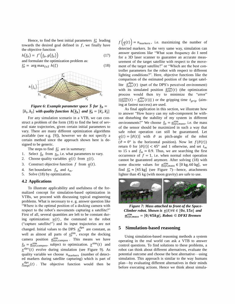
Hence, to find the best initial parameters �̂�0∗ leading
towards the desired goal defined in 𝑓, we finally have
the objective function
ℎ(�̂�0) = 𝑓′ (�̂�0, 𝑔(�̂�0)) (17)
and formulate the optimization problem as:
�̂�0∗ = arg max𝜉∈�̂� ℎ(𝜉) (18)
Figure 6: Example parameter space �̂� for �̂�𝟎 =
[�̂�𝟏, �̂�𝟐] with quality function 𝒉(�̂�𝟎) and �̂�𝟎∗ = [�̂�𝟏
∗ , �̂�𝟐∗ ]
For any simulation scenario in a VTB, we can con-
struct a problem of the form (18) to find the best of sev-
eral state trajectories, given certain initial parameters to
vary. There are many different optimization algorithms
available (see e.g. [9]), however we do not specify a
certain method since the approach shown here is de-
signed to be generic.
The steps to find �̂�0∗ are in summary:
1. Select �̂�0 from 𝑠0, i.e. what parameters to vary.
2. Choose quality variables 𝑞(𝑡) from 𝑠(𝑡).
3. Construct objective function 𝑓 from 𝑞(𝑡).
4. Set boundaries 𝑓𝑚 and 𝑡𝑚.
5. Solve (18) by optimization.
4.2 Applications
To illustrate applicability and usefulness of the for-
malized concept for simulation-based optimization in
VTBs, we proceed with discussing typical engineering
problems. What is necessary to e. g. answer question like
“Where is the optimal position of a docking camera with
respect to the robot’s movements capturing a satellite?”
First of all, several quantities are left to be constant dur-
ing optimization: 𝑢(𝑡) , the command to the robot
(“capture satellite!”) and its input trajectories are not
changed. Initial values to the DPS 𝑠0dps
are constant, as
well as almost all parts of 𝑠0sim , except the docking
camera position 𝑎sys,campossim . This means we have
�̂�0 = 𝑎sys,campossim , subject to optimization. 𝑥sim(𝑡) and
𝑥𝑑𝑝𝑠(𝑡) evolve during simulation (see Figure 9). As
quality variable we choose 𝑛markers (number of detect-
ed markers during satellite capturing) which is part of
𝑥impldps (𝑡) . The objective function would then be
𝑓 (𝑞(𝑡)) = 𝑛markers , i.e. maximizing the number of
detected markers. In the very same way, simulation can
answer questions like “What scan frequency do I need
for a 3D laser scanner to guarantee an accurate meas-
urement of the target satellite with respect to the move-
ment of the target satellite?” or “Which are the best con-
troller parameters for the robot with respect to different
lighting conditions?”. Here, objective functions like the
comparison of the estimated position of the target satel-
lite �̂�envdps
(𝑡) (part of the DPS’s perceived environment)
with its simulated position �̂�envsim(𝑡) (the optimization
process would then try to minimize the “error”
||�̂�envsim(𝑡) − �̂�env
dps(𝑡)|| ) or the gripping time 𝑡𝑔𝑟𝑖𝑝 (aim-
ing at fastest success) are used.
As final application in this section, we illustrate how
to answer “How heavy can my sub-component be with-
out disturbing the stability of my system in different
environments?” We choose �̂�0 = 𝑎sys,masssim , i.e. the mass
of the sensor should be maximized in such a way that
safe robot operation can still be guarantueed. Let
𝑞(𝑡) = [𝜗(𝑡)] with 𝜗 as pitch-angle of the robot
(𝜗 = 0° is the horizontal position). Now let 𝑓(𝜗(𝑡))
return 0 for |𝜗(𝑡)| < 45° and 1 otherwise, and set 𝑡𝑚
to 15 s and 𝑓𝑚 = 0.9. Thus, we are searching the first
occurrence of 𝑓 = 1, i.e. when normal robot operation
cannot be guaranteed anymore. After solving (18) with
some discrete values for 𝑎sys,masssim ∈ [0 kg, 60 kg], we
find �̂�0∗ ≈ [45 kg] (see Figure 7)—hence, attachments
lighter than 45 kg (with moon gravity) are safe to use.
Figure 7: Mass attached to front of the Space-
Climber robot. Shown is 𝒔(𝒕)∀𝒕 ∈ [𝟎𝒔, 𝟏𝟓𝒔] and
𝒂𝒔𝒚𝒔,𝒎𝒂𝒔𝒔𝒔𝒊𝒎 = [𝟎/𝟒𝟓𝒌𝒈]. Robot: © DFKI Bremen
5 Simulation-based reasoning
Using simulation-based reasoning methods a system
operating in the real world can ask a VTB to answer
control questions. To find solutions to these problems, a
robot can think about different alternatives, evaluate the
potential outcome and choose the best alternative—using
simulation. This approach is similar to the way humans
plan—by evaluating different alternatives in their minds
before executing actions. Hence we think about simula-
tion as a “mental model” [10] for intelligent robots.
The so-called Sense-Think-Act-paradigm [11] is
considered as the operational definition of an autono-
mous robot. As the Sense-Think-Act-paradigm is based
upon our understanding of human behavior, also the
‘‘thinking process’’ of robots should be based upon hu-
man reasoning. Humans construct mental models from
perception and experience. Using these models, they can
consider and review various action alternatives and their
outcomes.
5.1 Basic concept
To this end, it must be possible to reproduce the full
Sense-Think-Act-Cycle in simulation. Analogous to the
human mental model, this requires a virtual model of the
robot and its environment. The concept for simula-
tion-based reasoning is very similar to that of simula-
tion-based optimization from section 4. However, in this
case the optimization goal is to find the best input signal
𝑢(𝑡), e.g. a command to the satellite or a robot trajectory.
In terms of decision theory, the system now has to find
the best decision 𝑑opt itself, during real operation. This
is only possible when the whole VTB is available
“on-board” and the DPS is implemented as part of the
VTB (or directly connected to it) as shown in Figure 4.
The whole robotic system—or just a particular DPS
component as part of it—can then toggle the switches
𝑇sense and 𝑇act from real to simulation mode. All bene-
fits of simulation-based optimization are now available
to the DPS itself. Different action alternatives 𝑢(𝑡) can
now be evaluated or simply tried in simulation, without
the risk of real failure.
When formalizing this approach, the input signal
𝑢(𝑡) takes the role of �̂�0 from section 4.1. In order to
produce meaningful results, the VTB’s simulated envi-
ronment must of course be realistic, at least in relevant
properties. This may be achieved by providing the VTB
with an “a priori” environmental model.
5.2 Applications
The first example features a mobile exploration robot
which is located at the bottom of a crater, and the mis-
sion objective is to reach the crater’s rim. If only one
command 𝑢(𝑡) can be sent to the robot to start moving,
we look for the best starting direction 𝜑 of the robot in
order to fulfill its mission. A solution to the optimization
problem should yield a robot heading that will ensure a
robot trajectory to the top of the crater rim. We choose
�̂�0 = [𝜑] and 𝑞(𝑡) = 𝑧(𝑡) with 𝑧(𝑡) as the current
elevation of the robot. Then we can simply take
𝑓(𝑧(𝑡)) = 𝑧(𝑡) as objective function, since the crater
rim is the highest location in the given environment. 𝑡𝑚
has to be long enough (in this case several minutes),
while 𝑓𝑚 is not strictly needed and can be set
to 𝑓𝑚 = ∞ (or any value much higher than 𝑧(𝑡) is
likely to take). After solving (18) with some discrete
values for 𝜑 ∈ [−45°, 45°] , we find that �̂�0∗ = [0°]
works well (see Figure 8).
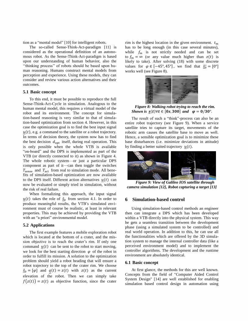
Figure 8: Walking robot trying to reach the rim.
Shown is 𝒔(𝒕)∀𝒕 ∈ [𝟎𝒔, 𝟑𝟎𝟎] and 𝝋 = 𝟎/𝟑𝟎°.
The result of such a “think”-process can also be an
entire robot trajectory (see Figure 9). When a service
satellite tries to capture its target, movements of the
robotic arm causes the satellite base to move as well.
Hence, a sensible optimization goal is to minimize these
base disturbances (i.e. minimize deviations in attitude)
by finding a better suited trajectory 𝑢(𝑡).
Figure 9: View of Galileo IOS satellite through
camera simulation [12], Robot capturing a target [13]
6 Simulation-based control
Using simulation-based control methods an engineer
then can integrate a DPS which has been developed
within a VTB directly into the physical system. This way
he gets a seamless transition between the development
phase (using a simulated system to be controlled) and
real world operation. In addition to this, he can use all
the functionalities which are offered by the 3D simula-
tion system to manage the internal controller data (like a
perceived environment model) and to implement the
controller algorithms. The development and the runtime
environment are absolutely identical.
6.1 Basic concept
At first glance, the methods for this are well known.
Concepts from the field of "Computer Aided Control
System Design" [14] are well established for enabling
simulation based control design in automation using
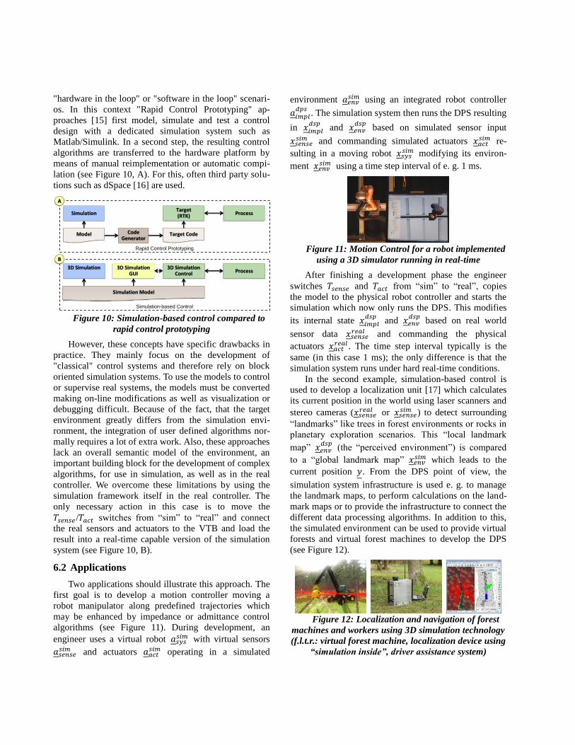
"hardware in the loop" or "software in the loop" scenari-
os. In this context "Rapid Control Prototyping" ap-
proaches [15] first model, simulate and test a control
design with a dedicated simulation system such as
Matlab/Simulink. In a second step, the resulting control
algorithms are transferred to the hardware platform by
means of manual reimplementation or automatic compi-
lation (see Figure 10, A). For this, often third party solu-
tions such as dSpace [16] are used.
Figure 10: Simulation-based control compared to
rapid control prototyping
However, these concepts have specific drawbacks in
practice. They mainly focus on the development of
"classical" control systems and therefore rely on block
oriented simulation systems. To use the models to control
or supervise real systems, the models must be converted
making on-line modifications as well as visualization or
debugging difficult. Because of the fact, that the target
environment greatly differs from the simulation envi-
ronment, the integration of user defined algorithms nor-
mally requires a lot of extra work. Also, these approaches
lack an overall semantic model of the environment, an
important building block for the development of complex
algorithms, for use in simulation, as well as in the real
controller. We overcome these limitations by using the
simulation framework itself in the real controller. The
only necessary action in this case is to move the
𝑇𝑠𝑒𝑛𝑠𝑒/𝑇𝑎𝑐𝑡 switches from “sim” to “real” and connect
the real sensors and actuators to the VTB and load the
result into a real-time capable version of the simulation
system (see Figure 10, B).
6.2 Applications
Two applications should illustrate this approach. The
first goal is to develop a motion controller moving a
robot manipulator along predefined trajectories which
may be enhanced by impedance or admittance control
algorithms (see Figure 11). During development, an
engineer uses a virtual robot 𝑎𝑠𝑦𝑠𝑠𝑖𝑚 with virtual sensors
𝑎𝑠𝑒𝑛𝑠𝑒𝑠𝑖𝑚 and actuators 𝑎𝑎𝑐𝑡
𝑠𝑖𝑚 operating in a simulated
environment 𝑎𝑒𝑛𝑣𝑠𝑖𝑚 using an integrated robot controller
𝑎𝑖𝑚𝑝𝑙𝑑𝑝𝑠
. The simulation system then runs the DPS resulting
in 𝑥𝑖𝑚𝑝𝑙𝑑𝑠𝑝
and 𝑥𝑒𝑛𝑣𝑑𝑠𝑝
based on simulated sensor input
𝑥𝑠𝑒𝑛𝑠𝑒𝑠𝑖𝑚 and commanding simulated actuators 𝑥𝑎𝑐𝑡
𝑠𝑖𝑚 re-
sulting in a moving robot 𝑥𝑠𝑦𝑠𝑠𝑖𝑚 modifying its environ-
ment 𝑥𝑒𝑛𝑣𝑠𝑖𝑚 using a time step interval of e. g. 1 ms.
Figure 11: Motion Control for a robot implemented
using a 3D simulator running in real-time
After finishing a development phase the engineer
switches 𝑇𝑠𝑒𝑛𝑠𝑒 and 𝑇𝑎𝑐𝑡 from “sim” to “real”, copies
the model to the physical robot controller and starts the
simulation which now only runs the DPS. This modifies
its internal state 𝑥𝑖𝑚𝑝𝑙𝑑𝑠𝑝
and 𝑥𝑒𝑛𝑣𝑑𝑠𝑝
based on real world
sensor data 𝑥𝑠𝑒𝑛𝑠𝑒𝑟𝑒𝑎𝑙 and commanding the physical
actuators 𝑥𝑎𝑐𝑡𝑟𝑒𝑎𝑙 . The time step interval typically is the
same (in this case 1 ms); the only difference is that the
simulation system runs under hard real-time conditions.
In the second example, simulation-based control is
used to develop a localization unit [17] which calculates
its current position in the world using laser scanners and
stereo cameras (𝑥𝑠𝑒𝑛𝑠𝑒𝑟𝑒𝑎𝑙 or 𝑥𝑠𝑒𝑛𝑠𝑒
𝑠𝑖𝑚 ) to detect surrounding
“landmarks” like trees in forest environments or rocks in
planetary exploration scenarios. This “local landmark
map” 𝑥𝑒𝑛𝑣𝑑𝑠𝑝
(the “perceived environment”) is compared
to a “global landmark map” 𝑥𝑒𝑛𝑣𝑠𝑖𝑚 which leads to the
current position 𝑦. From the DPS point of view, the
simulation system infrastructure is used e. g. to manage
the landmark maps, to perform calculations on the land-
mark maps or to provide the infrastructure to connect the
different data processing algorithms. In addition to this,
the simulated environment can be used to provide virtual
forests and virtual forest machines to develop the DPS
(see Figure 12).
Figure 12: Localization and navigation of forest
machines and workers using 3D simulation technology
(f.l.t.r.: virtual forest machine, localization device using
“simulation inside”, driver assistance system)
SimulationTarget(RTK) Process
3D SimulationGUI
3D SimulationControl Process
3D Simulation
Model Target CodeCodeGenerator
Simulation Model
A
Rapid Control Prototyping
B
Simulation-based Control
7 Conclusion
This paper introduces new concepts of simula-
tion-based optimization, reasoning, and control to the
emerging idea of Virtual Testbeds, rounding the eRobot-
ics approach. These concepts target the cost and time
efficient realization of intelligent and robust robotic
systems throughout the entire lifecycle starting from
concept and engineering phases to the implementation of
controllers on real hardware up to mission operation.
Using these concepts, an engineer can use the very same
simulation system for the development of a data pro-
cessing system (DPS, let it be a simple robot controller,
an intelligent sensor or an action planning system for a
mobile robot), virtual system integration, test and evalu-
ation as well as real world operation. The DPS can use
the entire simulation system for data management, algo-
rithm implementation and pre-simulations of the conse-
quences of design changes or action alternatives. The
basis is one single model of the DPS and the simulated
environment which is used for system optimization dur-
ing development as well as reasoning and control during
real world operation.
The basic idea is promising and has already proven
its feasibility in various applications so far. One focus of
our future work will be the use of highly parallel simula-
tion for optimization and reasoning. In addition to this,
keeping the engineer inside the optimization loop is
important. That’s why we work on interactive optimiza-
tion techniques and intuitively comprehensible visualiza-
tion means. Last but not least, we will continue our work
in providing verified and calibrated close-to-reality sim-
ulation algorithms for various aspects (sensors, actuators,
rigid-body dynamics, process simulations, etc.).
Acknowledgments
iBOSS-2 and INVIRTES are funded by the German
Aerospace Center (DLR) with funds provided by the
Federal Ministry of Economics and Technology (BMWi)
under grant number 50 RA 1203 and 50 RA 1306.
References
[1] Y.-H. Yoo, T. Jung, M. Roemmermann, M. Rast, F.
Kirchner and J. Rossmann, "Developing a Virtual
Environment for Extraterrestrial Legged Robot with
Focus on Lunar Crater Exploration," in i-SAIRAS,
Sapporo, 2010.
[2] J. Rossmann, M. Schluse, M. Hoppen and R.
Waspe, "Integrating Semantic World Modeling, 3D
Simulation, Virtual Reality and Remote Sensing
Techniques for a new Class of Interactive
GIS-based Simulation Systems," in Geoinformatics,
Fairfax, USA, 2009.
[3] J. Roßmann, M. Schluse, C. Schlette and R. Waspe,
"A New Approach to 3D Simulation Technology as
Enabling Technology for eRobotics," in 1st
International Simulation Tools Conference & EXPO
2013, SIMEX'2013, Brussels, 2013.
[4] G. Deng, Simulation-based optimization, University
of Wisconsin: PhD Thesis, 2007.
[5] A. M. Law and M. G. McComas, "Simulation
optimization: simulation-based optimization," in
Proc. WSC, San Diego, California, 2002.
[6] M. C. Fu, "Optimization for simulation: Theory vs.
Practice," INFORMS Journal on Computing, vol.
14, no. 3, pp. 192-215, 2002.
[7] M. H. DeGroot, Optimal statistical decisions,
McGraw-Hill Book Company, 1970.
[8] B. P. Zeigler, H. Praehofer and T. G. Kim, Theory of
Modeling and Simulation, Second Edition,
Academic Press, 2000.
[9] J. Nocedal and S. J. Wright, Numerical
Optimization, New York: Springer, 1999.
[10] J. Roßmann, E. Guiffo Kaigom, L. Atorf, M. Rast,
G. Grinshpun and C. Schlette, "Mental Models for
Intelligent Systems: eRobotics Enables New
Approaches to Simulation-Based AI," KI -
Künstliche Intelligenz, pp. 1-10, 2014.
[11] M. Siegel, "The sense-think-act paradigm revisited,"
Robotic Sensing, 2003.
[12] J. Roßmann, N. Hempe, M. Emde and T. Steil, "A
Real-Time Optical Sensor Simulation Framework
for Development and Testing of Industrial and
Mobile Robot Applications" in ROBOTIK, 2012.
[13] E. Kaigom, T. Jung and J. Rossmann, "Optimal
Motion Planning of a Space Robot with Base
Disturbance," in ASTRA, Noordwijk, NL, 2010.
[14] M. Brdys and K. Malinowski, "Computer Aided
Control System Design:," World Scientific, 1994.
[15] D. Abel and A. Bollig, Rapid Control Prototyping,
Springer-Verlag, 2006.
[16] www.dspace.com. [Accessed 02 04 2014].
[17] M. Emde, B. Sondermann and J. Rossmann, "A
Self-Contained Localization Unit for Terrestrial
Applications and its Use in Space Environments," in
i-SAIRAS, Montreal, 2014.