1 Simulation Handouts PortaCom is in the process to evaluate profitability and potential risk of loss for a new printer with innovative designs. Preliminary marketing and financial analysis show as follows: Parameter (constant) Inputs Probabilistic or variable inputs Selling Price Per Unit $249 Direct Labor Cost/Unit $45 Administrative Cost $400,000 Parts Cost /Unit $90 Advertising Cost $600,000 First Year Demand (Units) 15,000 Base Case Scenario: What if Analysis Worst Best Direct Labor Cost/Unit $47 $43 Parts Cost /Unit $100 $80 First Year Demand (Units) 1,500 28,500 Estimate First Year Profitability Random Number Generation and Probability Distribution Direct Labor Cost/Unit Probability Parts Cost (Uniform Distribution) Demand (Normal Distribution) $43 0.1 Smallest Value $80 Mean () 15,000 $44 0.2 Largest Value $100 Std Deviation (s) 4,500 $45 0.4 $46 0.2 $47 0.1 Sum 1.0
Transcript
1
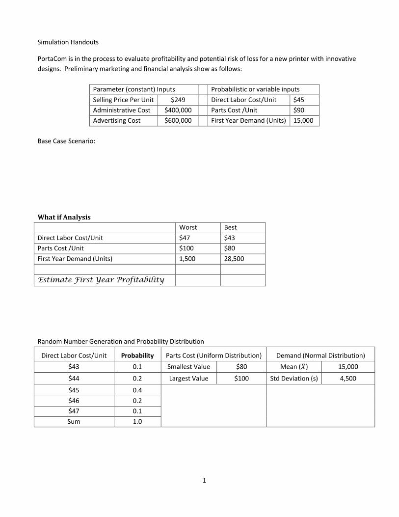
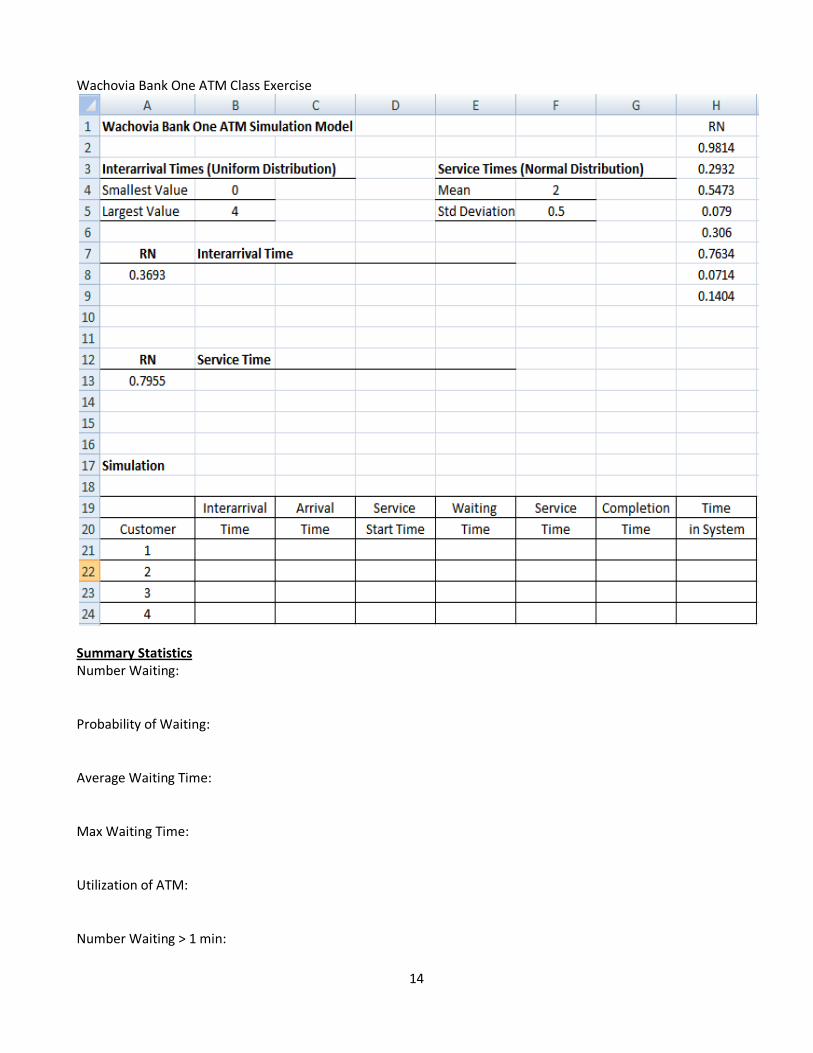
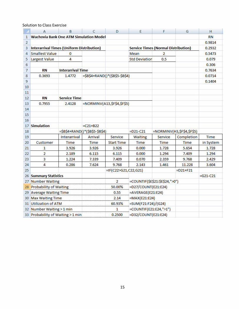
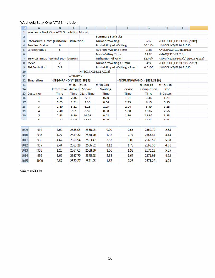
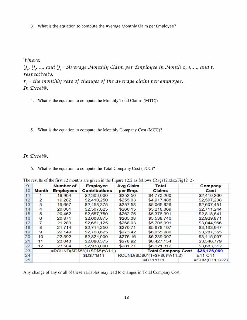
Simulation Handouts
PortaCom is in the process to evaluate profitability and potential risk of loss for a new printer with innovative
designs. Preliminary marketing and financial analysis show as follows:
Parameter (constant) Inputs Probabilistic or variable inputs
Selling Price Per Unit $249 Direct Labor Cost/Unit $45
Administrative Cost $400,000 Parts Cost /Unit $90
Advertising Cost $600,000 First Year Demand (Units) 15,000
Base Case Scenario:
What if Analysis
Worst Best
Direct Labor Cost/Unit $47 $43
Parts Cost /Unit $100 $80
First Year Demand (Units) 1,500 28,500
Estimate First Year Profitability
Random Number Generation and Probability Distribution
Direct Labor Cost/Unit Probability Parts Cost (Uniform Distribution) Demand (Normal Distribution)
$43 0.1 Smallest Value $80 Mean (��) 15,000
$44 0.2 Largest Value $100 Std Deviation (s) 4,500
$45 0.4
$46 0.2
$47 0.1
Sum 1.0
2
Summary Statistics
3
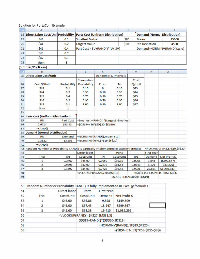
Solution for PortaCom Example
(Sim.xlsx/PortCom)
4
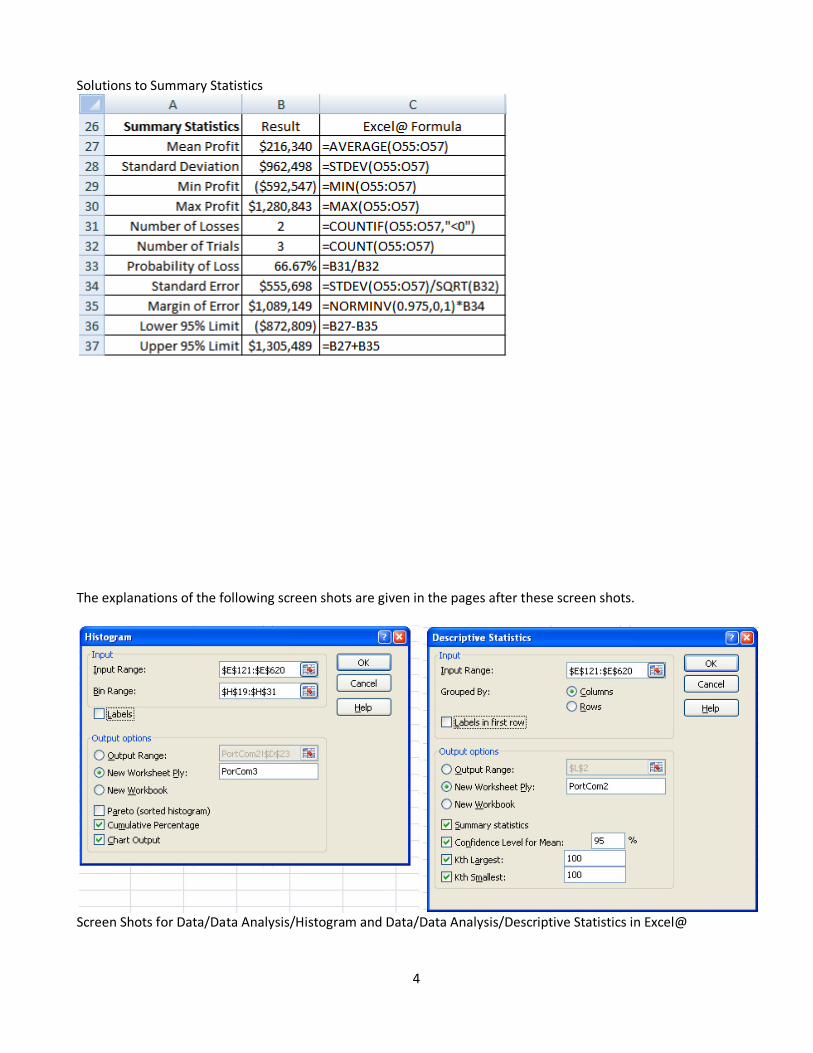
Solutions to Summary Statistics
The explanations of the following screen shots are given in the pages after these screen shots.
Screen Shots for Data/Data Analysis/Histogram and Data/Data Analysis/Descriptive Statistics in Excel@
5
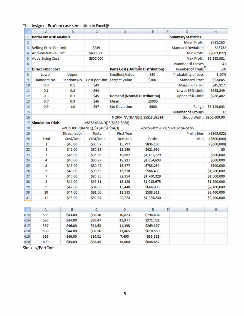
The design of ProCom case simulation in Excel@
Sim.xlsx/PortCom
6
The output of Descriptive Statistics and Histogram:
7
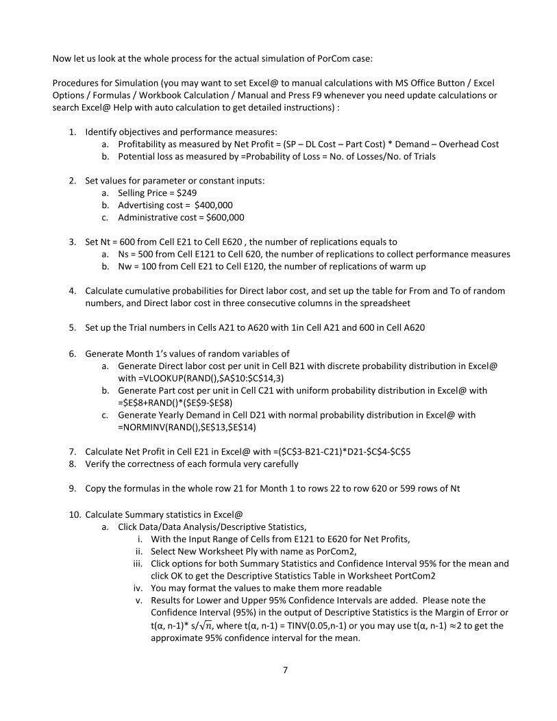
Now let us look at the whole process for the actual simulation of PorCom case:
Procedures for Simulation (you may want to set Excel@ to manual calculations with MS Office Button / Excel
Options / Formulas / Workbook Calculation / Manual and Press F9 whenever you need update calculations or
search Excel@ Help with auto calculation to get detailed instructions) :
1. Identify objectives and performance measures:
a. Profitability as measured by Net Profit = (SP – DL Cost – Part Cost) * Demand – Overhead Cost
b. Potential loss as measured by =Probability of Loss = No. of Losses/No. of Trials
2. Set values for parameter or constant inputs:
a. Selling Price = $249
b. Advertising cost = $400,000
c. Administrative cost = $600,000
3. Set Nt = 600 from Cell E21 to Cell E620 , the number of replications equals to
a. Ns = 500 from Cell E121 to Cell 620, the number of replications to collect performance measures
b. Nw = 100 from Cell E21 to Cell E120, the number of replications of warm up
4. Calculate cumulative probabilities for Direct labor cost, and set up the table for From and To of random
numbers, and Direct labor cost in three consecutive columns in the spreadsheet
5. Set up the Trial numbers in Cells A21 to A620 with 1in Cell A21 and 600 in Cell A620
6. Generate Month 1’s values of random variables of
a. Generate Direct labor cost per unit in Cell B21 with discrete probability distribution in Excel@
with =VLOOKUP(RAND(),$A$10:$C$14,3)
b. Generate Part cost per unit in Cell C21 with uniform probability distribution in Excel@ with
=$E$8+RAND()*($E$9-$E$8)
c. Generate Yearly Demand in Cell D21 with normal probability distribution in Excel@ with
=NORMINV(RAND(),$E$13,$E$14)
7. Calculate Net Profit in Cell E21 in Excel@ with =($C$3-B21-C21)*D21-$C$4-$C$5
8. Verify the correctness of each formula very carefully
9. Copy the formulas in the whole row 21 for Month 1 to rows 22 to row 620 or 599 rows of Nt
10. Calculate Summary statistics in Excel@
a. Click Data/Data Analysis/Descriptive Statistics,
i. With the Input Range of Cells from E121 to E620 for Net Profits,
ii. Select New Worksheet Ply with name as PorCom2,
iii. Click options for both Summary Statistics and Confidence Interval 95% for the mean and
click OK to get the Descriptive Statistics Table in Worksheet PortCom2
iv. You may format the values to make them more readable
v. Results for Lower and Upper 95% Confidence Intervals are added. Please note the
Confidence Interval (95%) in the output of Descriptive Statistics is the Margin of Error or
t(α, n-1)* s/√�, where t(α, n-1) = TINV(0.05,n-1) or you may use t(α, n-1) ≈2 to get the
approximate 95% confidence interval for the mean.
8
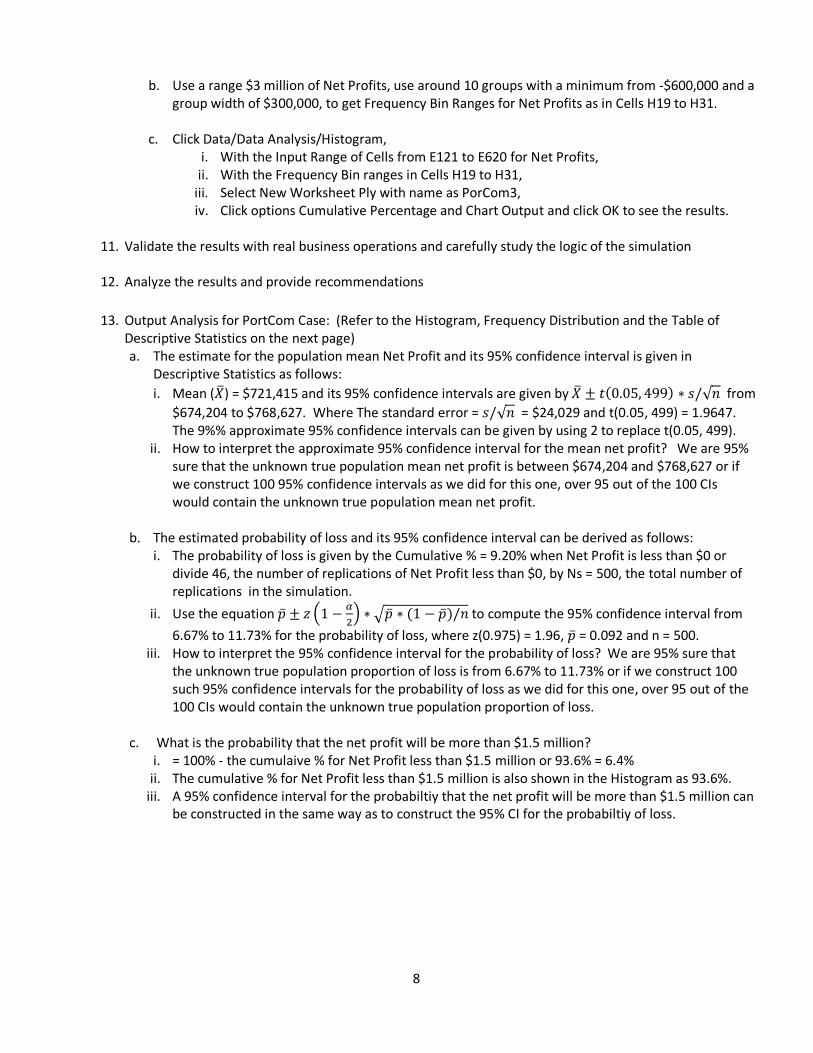
b. Use a range $3 million of Net Profits, use around 10 groups with a minimum from -$600,000 and a
group width of $300,000, to get Frequency Bin Ranges for Net Profits as in Cells H19 to H31.
c. Click Data/Data Analysis/Histogram,
i. With the Input Range of Cells from E121 to E620 for Net Profits,
ii. With the Frequency Bin ranges in Cells H19 to H31,
iii. Select New Worksheet Ply with name as PorCom3,
iv. Click options Cumulative Percentage and Chart Output and click OK to see the results.
11. Validate the results with real business operations and carefully study the logic of the simulation
12. Analyze the results and provide recommendations
13. Output Analysis for PortCom Case: (Refer to the Histogram, Frequency Distribution and the Table of
Descriptive Statistics on the next page)
a. The estimate for the population mean Net Profit and its 95% confidence interval is given in
Descriptive Statistics as follows:
i. Mean (��) = $721,415 and its 95% confidence intervals are given by �� ± ��0.05, 499� ∗ �/√� from
$674,204 to $768,627. Where The standard error = �/√� = $24,029 and t(0.05, 499) = 1.9647.
The 9%% approximate 95% confidence intervals can be given by using 2 to replace t(0.05, 499).
ii. How to interpret the approximate 95% confidence interval for the mean net profit? We are 95%
sure that the unknown true population mean net profit is between $674,204 and $768,627 or if
we construct 100 95% confidence intervals as we did for this one, over 95 out of the 100 CIs
would contain the unknown true population mean net profit.
b. The estimated probability of loss and its 95% confidence interval can be derived as follows:
i. The probability of loss is given by the Cumulative % = 9.20% when Net Profit is less than $0 or
divide 46, the number of replications of Net Profit less than $0, by Ns = 500, the total number of
replications in the simulation.
ii. Use the equation �� ± � �1 − ��� ∗ ��� ∗ �1 − ���/� to compute the 95% confidence interval from
6.67% to 11.73% for the probability of loss, where z(0.975) = 1.96, �� = 0.092 and n = 500.
iii. How to interpret the 95% confidence interval for the probability of loss? We are 95% sure that
the unknown true population proportion of loss is from 6.67% to 11.73% or if we construct 100
such 95% confidence intervals for the probability of loss as we did for this one, over 95 out of the
100 CIs would contain the unknown true population proportion of loss.
c. What is the probability that the net profit will be more than $1.5 million?
i. = 100% - the cumulaive % for Net Profit less than $1.5 million or 93.6% = 6.4%
ii. The cumulative % for Net Profit less than $1.5 million is also shown in the Histogram as 93.6%.
iii. A 95% confidence interval for the probabiltiy that the net profit will be more than $1.5 million can
be constructed in the same way as to construct the 95% CI for the probabiltiy of loss.
9
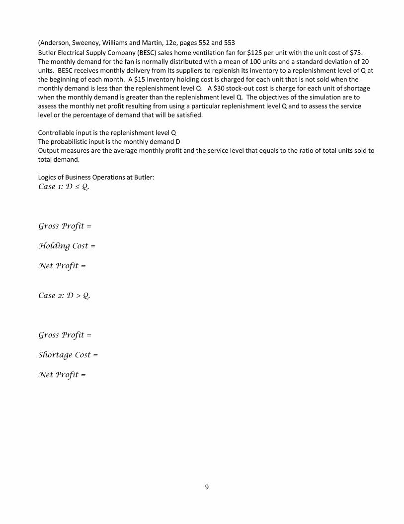
(Anderson, Sweeney, Williams and Martin, 12e, pages 552 and 553
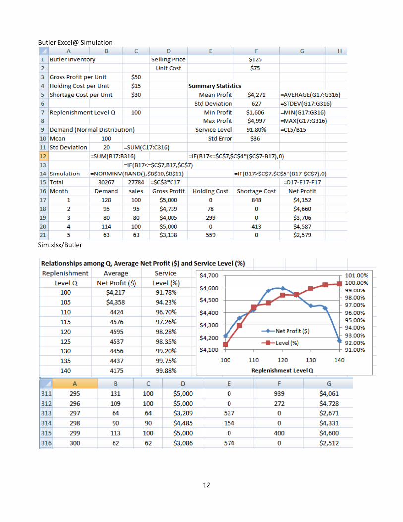
Butler Electrical Supply Company (BESC) sales home ventilation fan for $125 per unit with the unit cost of $75.
The monthly demand for the fan is normally distributed with a mean of 100 units and a standard deviation of 20
units. BESC receives monthly delivery from its suppliers to replenish its inventory to a replenishment level of Q at
the beginning of each month. A $15 inventory holding cost is charged for each unit that is not sold when the
monthly demand is less than the replenishment level Q. A $30 stock-out cost is charge for each unit of shortage
when the monthly demand is greater than the replenishment level Q. The objectives of the simulation are to
assess the monthly net profit resulting from using a particular replenishment level Q and to assess the service
level or the percentage of demand that will be satisfied.
Controllable input is the replenishment level Q
The probabilistic input is the monthly demand D
Output measures are the average monthly profit and the service level that equals to the ratio of total units sold to
total demand.
Logics of Business Operations at Butler:
Case 1: D ≤ Q. Gross Profit = Holding Cost = Net Profit = Case 2: D > Q. Gross Profit = Shortage Cost = Net Profit =