SIMULATION MODELING AND ANALYSIS OF ... - Bilkent · PDF filesimulation modeling and analysis...

SIMULATION MODELING AND ANALYSIS OF

BORDER SECURITY SYSTEM

A THESIS

SUBMITTED TO THE DEPARTMENT OF

INDUSTRIAL ENGINEERING

AND THE INSTITUTE OF ENGINEERING AND SCIENCE

OF BILKENT UNIVERSITY

IN PARTIAL FULFILMENT OF THE REQUIREMENTS

FOR THE DEGREE OF

MASTER OF SCIENCE

By

Gökhan ÇELİK

July, 2002

II

I certify that I have read this thesis and in my opinion it is fully adequate, in scope and in

quality, as a thesis for the degree of Master of Science.

..................................................................................................

Assoc. Prof. İhsan Sabuncuoğlu (Principal Advisor)



...................................................................................................

Assoc. Prof. Osman Oğuz



.....................................................................................................

Prof. Erdal Erel

Approved for the Institute of Engineering and Science

..........................................................................................

Prof. Mehmet Baray

Director of Institute of Engineering and Sciences

III

ABSTRACT SIMULATION MODELING AND ANALYSIS OF BORDER SECURITY SYSTEM Gökhan Çelik M.S. in Industrial Engineering Supervisor: Assoc. Prof. İhsan Sabuncuoğlu July, 2002

Border control is vital to the security of the nation and its citizens. Hence, states all

around the world look at measures to increase the security of their borders. On the other

hand, increasing border security also brings significant financial costs.

In this study, the performance of a Border Company is analyzed by simulation

modeling of the operational activities of a Border Company supported by Border Battalion.

Our main objective is to find out more efficient ways of increasing border control and

security along the land borders of Turkey. To achieve this objective, we examine the border

security system structure and its components, observe the relationships between

performance measures, and find out effects of security elements on the system performance

measures. We also investigate system responses when changes implemented in the system

or new resources added, evaluate different alternatives that improve the performance

measures by using ranking/selection and multi-criteria decision-making procedures. The

model is developed by using ARENA simulation system and the results are analyzed by

using SPSS statistical package program. A comprehensive bibliography is also provided in

the thesis.

Key Words: Military Simulation, Border Security

IV

ÖZET HUDUT GÜVENLİK SİSTEMİNİN SİMÜLASYONLA MODELLENMESİ VE ANALİZİ Gökhan Çelik Endüstri Mühendisliği Bölümü Yüksek Lisans Danışman: Doç. Dr. İhsan Sabuncuoğlu Temmuz 2002

Sınır kontrolu bir millet ve vatandaşlarının güvenliği için hayati öneme sahiptir. Bu

sebeple, dünyadaki tüm devletler sınırlarının güvenliğini artırmak için önlemler

aramaktadırlar. Diğer taraftan, sınır güvenliğini artırmak önemli maliyetler getirmektedir.

Bu çalışmada, Hudut Taburu tarafından desteklenen bir Hudut Bölüğü’nün harekata

yönelik faaliyetleri modellenerek, Hudut Bölüğü’nün performansı analiz edilmektedir. Ana

hedefimiz, Türkiye’nin kara sınırları boyunca sınır güvenliğini ve kontrolunu artırmak için

daha etkin yöntemler ortaya çıkarmaktır. Bu amacımıza ulaşmak için, hudut güvenlik

sisteminin yapısı ve bu sistemin bileşenleri incelenmekte, performans ölçütleri arasındaki

ilişkiler gözlemlenmekte ve güvenlik elemanlarının sistem performans ölçütleri üzerindeki

etkisi tespit edilmektedir. Ayrıca, sistemde değişiklikler yapıldığında veya yeni kaynaklar

ilave edildiğinde sistemdeki etkileri incelenmekte, performans ölçütlerini geliştiren değişik

alternatifler sıralama/seçme ve çok amaçlı karar verme yöntemleriyle

değerlendirilmektedir. Model ARENA simülasyon programı kullanılarak hazırlanmıştır.

İlgili referanslar tezde verilmiş bulunmaktadır.

Anahtar Sözcükler: Askeri Simülasyon, Hudut Güvenliği

V

To my wife Sena

VI

ACKNOWLEDGEMENT

I would like to express my deep gratitude to Dr. İhsan Sabuncuoğlu for his

guidance, attention, understanding, motivating suggestions and patience throughout all this

work.

I am indebted to the readers Osman Oğuz and Erdal Erel for their valuable

comments, kindness and time.

I cannot fully express my gratitude and thanks to my parents and friends for their

care, support and encouragement. And special thanks to my wife for her moral support and

help during this study.

Gökhan ÇELİK

VII

CONTENTS 1. Introduction

1.1. Protection and Security of Land Borders in Turkey..............................................

1.1.1. Tasks of Border Troops................................................................................

1.1.2. Organization and Deployment of Border Troops..........................................

1.2. Border Security System…………………………………………………………..

1.3. Objectives and Scope of the Thesis.......................................................................

2. Literature Review

2.1. Border Security in the World..................................................................................

2.2. Simulation Methodology and Software…………………………………………...

2.3. Military Simulation…………………………………………………………….…

3. The Simulation Model

3.1. Formulation of the Problem and Planning the Study..............................................

3.2. Model Development................................................................................................

3.2.1. Conceptual Model........................................................................................

3.2.2. Logical Model..............................................................................................

3.2.3. Simulation Model (Computer Code)...........................................................

3.3. Input Data Analysis.................................................................................................

3.4. Model Verification and Validation.........................................................................

3.4.1. Verification of Model....................................................................................

3.4.2. Validation of Model......................................................................................

1 2 3 5 7 9 11 12 14 18 19 23 30 30 32 32 33

VIII

4. Experimentation and Output Data Analysis

4.1. Determination of Run-length and Number of Replications.....................................

4.2. Output Analysis of the System..............................................................................

4.2.1. Analysis of Degree of Controllability Performance Measure..................... 4.2.2. Analysis of Frequency of Controlling Performance Measure.....................

4.2.3. Analysis of Ratio of Illegal Infiltrations Caught Performance Measure.....

4.2.4. Analysis of Relationship Between Performance Measures.........................

4.2.4.1. Relationship Between Degree of Controllability and Ratio of

Illegal Infiltrations Caught Performance Measures………………

4.2.4.2. Relationship Between Frequency of Controlling and Ratio of

Illegal Infiltrations Caught Performance Measures……………….

4.3. Analysis of Effect of Each Security Element to ...............................................

4.3.1. 24 Factorial Design.....................................................................................

4.3.2 Paired-T Approach………………………………………………………

5. Design and Analysis of Experiments

5.1. 25 Factorial Design..............................................................................................

5.2. Implementation of Analysis of Variance............................................................

5.3. Interpretation of ANOVA Results of the Performance Measures......................

5.3.1. Interpretation of Main Effects and Interactions of Ratio of Illegal

Infiltrations Caught Performance Measure...................................................

5.3.2. Interpretation of Main Effects and Interactions of Degree of

Controllability Performance Measure……………………………………...

5.3.3. Interpretation of Main Effects and Interactions of Frequency of

Controlling Performance Measure…………………………………………

37 40 40 42 45 47 48 51 54 54 56 59 61 66 67 71 73

IX

6. Alternatives and Border Security System Model in the Support of

Decision-making Process

6.1. Alternatives...........................................................................................................

6.2. Evaluation of Alternatives by Using Ranking and Selection Procedures............

6.2.1. All Pairwise Comparisons………………………………………………. 6.2.2. Rinott’s Procedure……………………………………………………….

6.3. Implementation of Geometric Mean Technique for our Multi-criteria

Decision-making Problem……………………………………….……………

7. Conclusion

7.1. Summary............................................................................................................... 7.2. Conclusions and Future Research Directions....................................................... Appendix A Confidence Intervals...................................................................................................

B 24 Factorial Design Experiments and ANOVA results ..............................................

C 25 Factorial Design Experiments and ANOVA results................................................

D Assumptions of ANOVA............................................................................................

E Results of Alternatives and Pair wise Comparisons of Alternatives..........................

F Computer Code of Border Security System................................................................

G Input Data...................................................................................................................

Bibliography...............................................................................................................

80 81 81 85 87 91 92 97 105 109 119 123 127 129 135

X

List of Figures Figure 1.1. Main organization scheme of Border Troops................................................

Figure 1.2. The scheme of deployment........................................................................... Figure 3.1. Schematic view of border security system model development...................

Figure 3.2. The General Flowchart of the Logical Model................................................

Figure 3.3. The Flowchart of Askarad..............................................................................

Figure 3.4. The Flowchart of Thermal Camera................................................................

Figure 3.5. The Flowchart of Patrols................................................................................

Figure 3.6. The Flowchart of Ambushes.......................................................................... Figure 3.7. The Flowchart of Illegal Infiltrations............................................................. Figure 3.8. Fault Insertion Test......................................................................................... Figure 3.9. Failure Insertion Test..................................................................................... Figure 3.10. Comparison of Simulation Model Results and Calculations made by hand.

Figure 3.11. A Sight of Animation of the Simulation Model............................................

Figure 4.1. Determination of run-length.........................................................................

Figure 4.2. Distribution of Degree of Controllability......................................................

Figure 4.3. Distribution of Frequency of Controlling...................................................... Figure 4.4. Distribution of Ratio of Illegal Infiltrations Caught......................................

Figure 4.5. Distribution of Ratio of Illegal Infiltrations Caught...................................... Figure 4.6. Correlation Between Ratio of Illegal Infiltrations Caught and

Degree of Controllability...............................................................................

Figure 4.7. Relation Between Degree of Controllability and Ratio of Illegal

Infiltrations Caught……………………………………………….………..

Figure 4.8. Relation Between Performance Measures, Cost and Capacity of Resources

Figure 4.9. Relation Between Frequency of Controlling and Ratio of Illegal

Infiltrations Caught…………………………………………………….…..

Figure 4.10. Relation Between Performance Measures and Capacity of Patrols.......... Figure 4.11. Main Effect Diagram for Each Performance Measure…………………..... Figure 5.1. Histogram of residuals compared with normal for ratio of illegal

infiltrations caught ........................................................................................

Figure 5.2. Normal P-P of residuals for ratio of illegal infiltrations caught…………… Figure 5.3. Main effect diagram of factors for ratio of illegal infiltrations caught...........

4

4

19

24

25

26

27

28

29

34

34

35

36

38

41

43

45

46

48

50

51

53

53

57

65

66

67

XI

Figure 5.4. Interactions between factors for ratio of illegal infiltrations caught...............

Figure 5.5. Main effect diagram of factors for degree of controllability..........................

Figure 5.6. Interactions between factors for degree of controllability ............................

Figure 5.7. Main effect diagram of factors for frequency of controlling.........................

Figure 5.8. Main effect diagram of factors for frequency of controlling.........................

Figure 5.9. Interactions between factors for frequency of controlling ………………..

Figure 6.1. The pairwise comparisons of alternatives and ranking of alternatives for

ratio of illegal infiltrations caught performance measure..............................


degree of controllability performance measure..............................................


frequency of controlling performance measure.............................................

Figure 6.4. Hierarchy tree of alternatives and criteria....................................................

Figure C.1. Normal probability plot of performance measures.......................................

Figure D.1. Scatter plot of variances of performance measures.......................................

Figure D.2. Histogram of residuals compared with normal for performance measures...

Figure D.3. Normal P-P of residuals for performance measures......................................

Figure D.4. Scatter plot of residuals for performance measures......................................

70

71

72

73

74

76

83

83

84

87

118

119

121

121

122

XII

List of Tables Table 4.1. Desired Precisions............................................................................................

Table 4.2. Results of Two-stage Procedure.......................................................................

Table 4.3. Policies and results of performance measures..................................................

Table 4.4. Policies and results of performance measures..................................................

Table 4.5. Factors Effecting Border Security System.......................................................

Table 4.6. Levene Test Results..........................................................................................

Table 4.7 Bartlett Test Results..........................................................................................

Table 4.8. Paired Samples Test for Ratio of Illegal Infiltrations Caught…………….…

Table 4.9. Paired Samples Test for Degree of Controllability Performance Measure….…

Table 4.10. Paired Samples Test for Frequency of Controlling Performance Measure...

Table 5.1. Factors and levels of 25 factorial design..........................................................

Table 5.2. Bartlett test results for 25 factorial design......................................................

Table 5.3. Levene test results for 25 factorial design......................................................

Table 5.4. Independent Samples-t Test.............................................................................

Table 5.5. Bartlett Test Results for 24 Factorial Design..................................................

Table 5.6. Levene Test Results for 24 Factorial Design..................................................

Table 5.7. Interactions between factors for ratio of illegal infiltrations caught ..............

Table 5.8. Interactions between factors for degree of controllability……..……….….

Table 5.9. Interactions between factors for frequency of controlling…………………..

Table 5.10. Results of the factors affecting performance measures..…………………...

Table 6.1. Paired Samples Test of alternatives for ratio of illegal infiltrations caught...

Tables 6.2 Ranking of alternatives for ratio of illegal infiltrations caught.......................

Tables 6.3 Ranking of alternatives for degree of controllability......................................

Tables 6.4 Ranking of alternatives for frequency of controlling......................................

Table 6.5. Results of each alternative for each criterion..................................................

Table 6.6. Pair wise comparison matrix of criteria...........................................................

Table 6.7. Utility matrix………………………………………………………………...

Table 6.8. Weight matrix…………………………………………………………….….

Table 6.9. Values of alternatives.....................................................................................

Table 6.10. Ranking of alternatives..................................................................................

Table 7.1 Factors affecting the performance measures...................................................

38

39

49

52

54

55

55

58

58

58

60

62

62

63

64

64

69

72

75

77

82

85

85

86

88

88

89

89

90

90

93

XIII

Table 7.2 Factors and their descriptions..........................................................................

Table 7.3. Alternative description and ranking of alternatives.........................................

Table A.1a-A.8d. Confidence interval for performance measures of Border Company

and border platoons......................................................................................

TableB.1-B.3.Results, averages, variances of 10 replications for performance measures

Table B.4-B6. ANOVA results of performance measures………………………………

Table C.1-C.2. Factors and roles of factors for design points...........................................

Table C.3-C.5. Results, averages, variances of 10 replications for performance

measures ( 25 factorial design)..................................................................

Table C.6-C10. ANOVA results for each performance measure......................................

Table C.11. Analysis of normal P-P plots effects of performance measures....................

Table D.1. Residual analysis for performance measures.................................................

Table E.1-E.3. Results of 10 replications for performance measures of alternatives .......

Table E.4. Paired samples test of alternatives for degree of controllability…………...

Table E.5. Paired samples test of alternatives for frequency of controlling……….…..

Table E.6a-6d. Pairwise comparison matrix of alternatives for each criterion.................

Table G1-G18 Input data parameters................................................................................

93

94

97

105

107

109

110

113

117

120

123

124

125

126

129

1

CHAPTER 1 Introduction

It is a well-known fact that the border control is vital to the security of the nation

and its citizens. The threat of international terrorism, worldwide illegal immigration and

refugee problems, drug and arms smuggling are issues of that concerns states. Therefore,

all states in the world look at measures to increase security at their borders. They apply

different organizations and methods to protect their borders. But the main resources are

technology and personnel. Therefore, increasing border security is only possible by

increasing resources or improving methods. On the other hand, increasing resources

causes significant financial costs.

In our thesis, we investigate the possible ways of increasing border control and

security along the land borders of Turkey. First, we present brief information about how

Turkey protects her land borders.

1.1 . Protection and Security of Land Borders in Turkey

Turkey has land borders of 2852 kilometers long with neighbor countries (202 km

with Greece, 268 km with Bulgaria, 877 km with Syria, 378 km with Iraq, 528 km with

Iran, 17 km with Nahcıvan, 325 km with Armenia and 257 km with Georgia). In Turkey,

the task of protection of land borders and providing security along the borders was given

to the Land Forces by law at 10.11.1988. This task is executed by Border Troops.

2

1.1.1. Tasks of Border Troops

The tasks of border troops are as follows:

Peace Time

• To protect the land borders and to provide security along the borders in its

responsibility terrain.

• To prevent smuggling and related illegal activities.

• To prevent trans-borders crimes unauthorized entry into or exit from the

territory of Turkey (such as illegal infiltrations of refugees, terrorists,

smugglers, enemy special forces).

• To coordinate with civil administration.

• To get prepared for war according to general defense plans.

• Collection of intelligence.

War Time

• To execute tasks according to general defense plans.

To hold ground in less threatened sectors so long as the main

attack does not develop in a particular sector.

Protection of vital installations against enemy commandos and

paratroop raids.

Border troops execute their tasks under the light of laws, regulations, and rules of

our country, and treaties or protocols with the neighbor nations’ administrations.

3

1.1.2. Organization and Deployment of Border Troops

Border troops are organized by the proposals of Land Forces and approval of the

General Staff. Each border troop may have different organizations, which are determined

by order. Main organization scheme is shown in Figure 1.1. Border battalions consist of

three border companies and one headquarters company. Headquarters company supports

the activities of border battalion commander and his headquarters. It also provides

logistic support for border companies. Border companies are operational troops of border

battalion. It can be said that the main force that protects the land borders of Turkey are

border companies. Border companies consist of three border platoons and one center

platoon. Center platoon supports border company headquarters. Operational tasks such as

patrol and ambush are executed by border platoons. Sometimes center platoon supports

border platoons. Border troops are equipped with new technology and supported by

personnel to execute their tasks best.

Border troops are located in such a way that they execute their tasks best under

peace and war conditions. Any change of locations is under the authority of General

Staff. Unless permission is given, no change can be done in the location of border posts.

Brigade commanders determine the responsibility terrains of border troops.

Basically, border platoons (border posts) are located along the borders and border

companies that direct and manage the border platoons are located behind the platoons,

lastly border battalions are located behind the border companies. The scheme of

deployment is shown in Figure 1.2.

4

Border Battalion Headquarters Company Border Companies ... ... Headquarters and

Center platoon Border Platoons Figure 1.1. Main organization scheme of Border Troops

Figure 1.2. The scheme of deployment

......

...

... ...

......

. .. ...... ...

...

Border Battalion

Border Company Border CompanyBorder Company

Bd Platoon

Bd Platoon

Bd Platoon

Bd PlatoonBd Platoon



Bd PlatoonBd PlatoonBd Platoon

5

1.2. Border Security System

Border Security System consists of physical obstacles system and border

surveillance and controlling system. These complementary systems can be used as a

whole or they can be used partially depending on needs and possibilities. At this point,

the importance of the region, threat and structure of the terrain are considered.

The Ministries of Defense and Home Affairs are also responsible for installing

and maintenance of the physical obstacles system. These obstacles are:

• Fences along the borders, barbed wires (8 meters width along the borders).

• Track fields (7 meters width along the borders).

• Ways for patrols and illumination area (7 meters width along the borders).

Border surveillance and controlling system is the main part of the border security

system. Because it contains all active precautions against unauthorized entry into or exit

from the territory of Turkey. It is the basic means of providing security along the borders.

Border Patrols, ambushes, sentries, thermal cameras and askarad are the main elements

of this system.

Border Patrols: A patrol consists of three soldiers (one of them is the commander

of the patrol) and they execute their tasks by watching and controlling the areas on their

route along the borders. These soldiers belong to border platoons and they leave for task

from border posts in some time intervals, execute their tasks and return border posts.

They control the borders under day and night conditions.

Ambushes: An ambush consists of five-six soldiers under the command of

commissioned or non-commissioned officer. Ambushes may be stationary or mobile. If

they are stationary, they go to the place where they control the area through the night. If

6

they are mobile they change their places after execution of their task at one place. They

change their places 3 or 4 times and they stay at one place no more than 2-3 hours.

Ambushes may be equipped with night-vision devices. If they have night-vision devices,

the area that they control gets wider. Ambushes execute their tasks under night

conditions.

Sentries: Their main task is to watch the borderlines and enemy terrain. They

execute their tasks at watchtowers, which are constructed at some specific places along

the borders. Sentries are on duty under day conditions. Watching duty is executed by

using electronic systems such as askarad and thermal cameras under night conditions.

Thermal Cameras: Thermal Camera System is an infrared imaging system, which

enables the user target detection, recognition and observation capabilities in all weather

conditions. The passive nature of imaging provides fully covert surveillance. Light-

weight and portable structure, operability by one man, operability with 12-24 VDC

sealed lead acid battery or 220 VAC at stationary applications, minimum focusing range,

uninterrupted operation capability without being affected from poor field and weather

conditions, low noise level and perfect imaging make thermal camera an ideal system for

military purposes. Thermal cameras are used for; border surveillance, protection of

headquarters, military zones and port/harbor surveillance. Thermal Cameras are under

the control of Border Company. They can be used only under night conditions, stationary

or mobile.

Askarad: Askarad, ground surveillance radar, is a new generation radar system

used for surveillance of moving targets and for artillery fire adjustment in the battlefield.

Askarad combines surveillance, target acquisition and classification, target tracking and

artillery fire adjustment functions within one unit. Askarad is used for; surveillance,

7

target acquisition and moving target classification, precision location of targets, plotting

of targets on the display, adjustment of artillery fire, guidance of small ground or

airborne attack units, helicopter navigational aid especially for homing. Askarads are

under the control of Border Battalion. They can be used under day and night conditions,

as stationary or mobile.

Both thermal camera and askarad are electronic surveillance systems. Main

difference between them is the range that they are capable of control. Askarad is capable

of detecting targets from 4-5 times farther than that of thermal camera.

1.3. Objectives and Scope of the Thesis

In this thesis, our main aim is to investigate how to increase border control and

efficiency of border security along the borders of Turkey. To achieve our purpose, we

model the operational activities of border company supported by border battalion via

simulation. We first study border security system structure and its components. At this

stage, our aim is to assess the effectiveness of the system in terms of performance

measures such as the ratio of illegal infiltrations caught, degree of controllability and

frequency of controlling. Secondly, we attempt to understand the relationship between

security elements and performance measures. In other words, we observe the behavior of

the system and interactions of security elements and performance measures closer.

Thirdly, we investigate effect of each security element on the performance measures and

find out the degree of importance of each security element. Fourthly, we analyze the

significant factors that affect the performance measures. Fifthly, we investigate system

responses, when changes made in the system or new resources added to the system.

Lastly, we evaluate different alternatives that increase the performance measures, by

8

using ranking, selection and multi-criteria decision-making procedures. At the end, we

hope to find possible ways of increasing border security by a simulation model of the

system that can be used before implementing real investments in the system or real

decisions about the system.

The outline of the thesis is as follows. Chapter 2 presents the literature review

about border security systems in the world, simulation methodologies and military

simulations. In Chapter 3, we give the simulation model of border security system.

Verification and validation issues are also discussed in this section. In Chapter 4, the

system behavior is examined, the interactions of system components and performance

measures are found out and effects of each security element on the performance measures

are investigated. Chapter 5 presents experimental design and implementation of analysis

of variance procedure to find out the significant factors that affect the performance

measures. In Chapter 6, alternatives are examined, compared and they are ranked and

selected by using ranking and selection procedures and multi-objective decision-making

procedures. Chapter 7 gives conclusion of the study and future research directions.

9

CHAPTER 2 Literature Review

During our literature review, we search for the studies or researches that are

related with analysis of border security systems via simulation. We also search for how

to increase border security. Although there are some official studies those are about

precautions taken for more secure borders, we couldn’t meet any study that simulation

tool is used in the analysis of border security systems in the literature. Furthermore, we

observe that the border security systems vary from country to country, but the basic

components and operational activities of the systems are similar. Thus, we first give

information about border security systems from other countries and precautions taken for

more secure borders. Then, since we use simulation tool to analyze our border security

system, we search for simulation methodology and software. We also review the military

simulation studies to learn how to deal with the subject and to overcome the problems.

2.1. Border Security in the World

During our survey, we examine how the other countries protect their land borders.

There are mainly three kinds of organization that countries apply to protect their land

borders. One of them is giving this task to the Army. This method is used in our country

and in our neighbor countries. The second method is performing this task by state

organizations rather than Army. These organizations are under the control of civil

administration. An example of this method is U.S. Border Patrol organization that is

under the control of Immigration and Naturalization Service of Department of Justice.

Sometimes these organizations are supported by Army. The third method is execution of

10

this task by Police Forces. At wartime, these forces are under the operational control of

the Army. But at the peacetime, they are under the control of the Ministry of Home

Affairs. This method is applied in India and this organization is called as Border Security

Force.

As seen, when the border security is the subject under concern, the main

ministries, departments and armed forces of the states have responsibilities for security of

country borders. Therefore, besides many news those are related with border security of

countries from all around the world such as declarations of researches for more secure

borders or precautions and results of precautions in both technological and organizational

issues, we meet some official reports related with border security.

There are several reports of GAO (General Accounting Office is the investigative

arm of Congress in U.S.) and CRS (Congressional Research Service) related with border

control and security.

In their CRS report (June 18, 2001), William J. Krouse (Analyst in Social

Legislation; Domestic Social Policy Division) and Raphael F. Perl (Specialist in

International Affairs; Foreign Affairs, Defense, and Trade Division) explain the

importance of border security and propose some options to prevent illegal entry into the

United States.

In GAO reports, after making studies about border security, precautions are

proposed and results of precautions are evaluated. As precautions for strengthening the

border, (1) concentrating personnel and technology resources, starting first with the

sectors with the highest level of illegal infiltration activity and moving to the areas with

the least activity, (2) making maximum use of physical barriers to deter entry along the

border, (3) increasing the proportion of time Border Patrol agents spent on border control

11

activities and (4) identifying the appropriate quantity and mix of technology and

personnel needed to control the border, are proposed in some parts of GAO reports.

2.2. Simulation Methodology and Software

We use simulation tool to analyze border security system. Throughout our study,

we use the basic principles, which are stated in Shannon (1998), Banks (1998) and Mehta

(2000). In these studies, they explain how a complex simulation study of any discrete

system be executed efficiently and effectively following simple basic methodology.

Sargent (1999) discusses validation and verification of simulation models and

different approaches are presented to decide model validity. Robinson (1997) sets

simulation model verification and validation in the context of the process of performing a

simulation study. Balcı (1998) presents guidelines for conducting verification, validation

and accreditation of simulation models. Fifteen guiding principles are introduced and

many verification and validation techniques are presented. We verify and validate our

model by using techniques and considering the principles of Balcı (1998) for all steps of

our study.

Centeno and Reyes (1998) explain several concepts and techniques to analyze

output of the simulation model. Kelton (1997) explain methods to help design the runs

for simulation models and interpreting their outputs. Again, Kelton (1999) introduces

some of the ideas, issues, challenges, and opportunities in deciding how to experiment

with a simulation model to learn about its behavior. Montgomery (1992) explains design

and analysis of experimental design in his book. We use these studies in output analysis

and experimental design parts of our study.

12

Swisher and Jacobson (1999) presents a survey of the literature for two widely-

used statistical methods for selecting the best design from among a finite set of k

alternatives: ranking and selection and multiple comparison procedures. We use some of

the methods stated in this study in evaluation of alternatives.

Takus and Profozich (1997) explain that the Arena software is a flexible and

powerful tool that allows analysts to create animated simulation models that accurately

represent virtually any system. In our study, we use Arena software because of its desired

properties.

2.3. Military Simulation

Hill, Miller and McIntyre (2001) describe the military as a big user of discrete

event simulation models. They discuss the uses of military simulation and the issues

associated with military simulation to include categorizations of various types of military

simulation.

Garrabrants (1998) proposes an expansion of simulation system’s role to support

all levels of command and control functioning, especially staff planning after receipt of

orders and mission rehearsal. He points out that simulation system is a natural solution to

the commander’s need for a planning and rehearsal system to support his operational

planning efforts.

Smith (1998) identifies and explores the essential techniques for modern military

training simulations. His study provides a brief historical introduction followed by

discussions of system architecture, simulation interoperability, event and time

management, verification and validation and fundamental principles in modeling and

specific military domains.

13

Roland (1998) presents a panel of knowledgeable individuals who are filling

those decision-making roles. Major problems in the current state of modeling and

simulation development and use, major modeling and simulation opportunities and

challenges are discussed in the panel “The future of military simulation”. He categorizes

the military modeling and simulation as engineering models, analysis models and

training models.

Chew and Sullivan (2000) discusses the activities and tasks during the early

stages of model development and addresses each of the verification, validation and

accreditation efforts separately, along with its associated activities. Balcı, Ormsby, Carr

and Saadi (2000) provide guidance in developing and executing a comprehensive and

detailed verification, validation and accreditation plan throughout the entire modeling

and simulation application development life cycle. Hartley (1997) explains verification

and validation in military simulations and discusses the cost aspect of verification and

validation.

14

CHAPTER 3

The Simulation Model

3.1. Formulation of the Problem and Planning the Study

One of the most important aspects of simulation study is a careful statement of

the objectives. Our main objective is to investigate how to increase border control and

efficiency of border security along the borders of Turkey. We think that the use of

simulation and statistical procedures analyzing the border security system will help to

achieve our main objective. We have other objectives to achieve. These are: to make a

thorough examination of the border security system structure and its components,

observe the relationships between performance measures, analyze factors that effect the

performance measures, find out the ways to increase the performance measures, and

investigate system responses when changes made in the system or addition of resources

made to the system to improve the performances.

As we already know, it is always preferable to use analytical models whenever

possible. At first glance optimization models seem to be available for the modeling and

solution of the system. But border security system has dynamic behavior that the system

state changes over time. If we look from the point of performance measures, optimization

model will give solution for only one performance measure that is the maximum length

of border that could be under control with our resources one at a time. But our

performance measures depend on time, moving characteristics of security elements and

catching of illegal infiltrations that all these measures have stochastic features. As we

mention in objective statement of our study, our objectives are mostly related with

behavior examination of the border security system and its components. We also try to

15

investigate a wide variety of “what if ” questions about our system to improve the

performance measures. Consequently, when we look from the aspects of border security

system characteristics (i.e. dynamic behavior of system, stochastic features of events),

performance measures to be evaluated and objectives that motivate us to make such a

study, simulation is appropriate tool for our study.

The Border Security System Model is developed to:

• Make it possible for border security planners to model the responsibility terrain of

border troops with different deployment, organization, terrain conditions and

resources.

• Analyze performance of border troops along the borders in their responsibility

terrain in terms of performance measures.

• Make it easy to find the strong and weak sides along the borders.

• Help to see the results of precautions that are taken for weak points or to increase

the security in the responsibility terrain of troops.

• Display the effect of each type of security element on the performance measures

and allow determining priority for drilling and maintenance.

• Perform new policies, changes of organization or deployment before conducting

real decisions about the system.

• Perform cost management before conducting real investments.

By using this model, border security planners, border troop commanders can

accurately and efficiently examine the behavior of the system; they can easily see the

results of their precautions and use the model as a support of their decision-making

process. We try to answer the following research questions:

16

1. How efficient is the system if we consider the performance measures?

2. What are the relationships between security elements and performance measures?

3. What are the relationships between performance measures?

4. How much does each element effect performance measures?

5. What are the significant factors that affect the performance measures?

6. How much does it affect the system if coordination is established between

security elements?

7. How much do additional resources affect the performance measures of the

system?

8. Which parts of the border are strong and weak in terms of performance measures?

Explanation of Performance Measures:

There are mainly three performance measures as an output of the system:

1. Degree of Controllability (DOC) is the ratio of time that a zone is under control

by security elements in one-year time period. After it is calculated for each zone,

the average of all zones is considered as a performance measure.

2. Frequency of Controlling (FOC) shows how many different times any zone gets

under control by security elements in one-year time period. After it is calculated

for each zone the average of all zones is taken as a performance measure.

3. Ratio of Illegal Infiltrations Caught (ROIIC) shows the ratio of number caught

illegal infiltrations to the total number of caught and couldn’t be caught

infiltrations in one-year time period. The average of all zones is considered as a

performance measure.

17

Input/Output Process

(*)Decision variables and parameters are given in Table 3.1 p.31. X Y

Outputs of the model are the functions of random variables presented in Table

3.1. Among these random variables duty time of each security element, failures of high-

tech devices, determination of duty places are the main random variables that affect the

degree-of-controllability output whereas determination that patrols are motorized or on-

foot and determination of mobile or stationary characteristics of duty are the main

random variables that affect the frequency-of-controlling output. Arrivals of illegal

infiltrations, infiltration time for each type of illegal infiltrations affect ratio-of-illegal-

infiltrations-caught. But, the ratio-of-illegal-infiltrations-caught performance measure is

also affected by random variables that affect the degree-of-controllability and the

frequency-of-controlling performance measures. Briefly, when we consider the

operational behavior of the border security system with its all components, each decision

variable and parameter has an effect on each performance measure.

• *Decision variables

• *Parameters

Simulation Model

1. Degree of controllability (DOC)

2. Frequency of controlling (FOC)

3. Ratio of illegal infiltrations caught (ROIIC)

Real Life

Y=f(X)

18

Other performance measures that the model is capable of evaluating:

• Number of illegal infiltrations caught by type (refugees, terrorists, smugglers,

enemy special forces and enemy commando troops).

• Number of illegal infiltrations that couldn’t be caught by type.

• Number of security elements (askarad, patrols, thermal camera, ambushes) that

served during a year.

• Contributions of each security element to the system performance measures.

Data needs and stochastic factors are analyzed in the input data analysis section.

3.2. Model Development

First we develop a conceptual model of the system. At this stage, we determine

the parts of real-world system to be modeled to achieve our objectives. If we think the

border troops in real world, they have many activities other than border security. But all

other activities support the main task that is protection and security of borders. Thus, our

conceptual model is about the operational activities that border troops perform for

security of borders. We model the operational activities of border company supported by

border battalion. Based on this conceptual model, we then develop our logical and

simulation model. Figure 3.1 shows the schematic view of border security system model

development.

19

Figure 3.1. Schematic view of border security system model development

3.2.1. Conceptual Model

At this stage, we determine elements of system, their relationships, assumptions

and data requirements of the simulation model.

Entities of the system:

• Patrols.

• Ambushes.

• Thermal camera.

• Askarad.

• Illegal infiltrations.

• Zones.

Attributes of the system:

• The departure time of security elements from their locations.

• Type of illegal infiltrations.

REAL WORLD SYSTEM:Border Troops

ASSUMED SYSTEM:Border Company supported by Border Battalion

CONCEPTUAL MODEL:Operational Activities for Security of Borders

LOGICAL MODEL:Flowchart

SIMULATION MODEL: Siman programming language/ARENA Simulation Package

20

• Duty time for each security elements.

• Using of night-vision tools by ambushes.

• Patrol type.

• Moving or stationary characteristics of security elements.

• Security element type.

Events of the system:

• Departure of security elements from their locations.

• Arrivals of illegal infiltrations.

• Catching of illegal infiltrations.

• Changing places of duty for askarad, thermal camera and ambushes if they are

moving.

• Failures before and during operation of askarad and thermal camera.

• Controlling of zones by patrols on their route.

• Controlling of zones by askarad, thermal camera and ambushes.

• Ending of duty and returning to locations.

Activities of the system:

• Controlling of zones by each security element.

• Illegal infiltrations.

Exogenous Variables (Input variables)

• Decision variables (controllable variables) and parameters (uncontrollable

variables) are listed in the input data analysis section.

21

Endogenous Variables (Output variables):

State Variables:

• State of zones (under control or not).

• Number of illegal infiltrations caught for each type.

• Number of security elements in the system.

Performance measures:

• Degree of controllability.

• Frequency of controlling.

• Ratio of illegal infiltrations caught.

The assumptions of our model are:

• The system is considered under night conditions.

• The responsibility terrain of a typical border company is considered.

• There are four platoons directed by border company.

• Each border platoon has approximately 4-6 kilometers responsibility terrain.

• There is one thermal camera belonging to border company.

• There is one askarad belonging to border battalion and it serves to three border

companies. Askarad is under consideration when it comes to responsibility terrain

of border company that is in the model.

• Two of border platoons have capability of patrolling for two sides of its location.

Two of them have capability for one side.

• There is no intelligence of any infiltration.

• Each zone is considered as an area that can be controlled by patrol.

22

Night conditions vs. day conditions

We model the border security system under night conditions. Because, most of

the operational activities of border troops are performed under night conditions.

Electronic surveillance systems (askarad, thermal camera), ambushes equipped with

night-vision tools and patrols are the main security elements used for border control

under night conditions. On the other hand, sentries and patrols under day conditions

perform border control. Since the visibility is high under day conditions, sentries

stationed at watchtowers control wide part of border. Therefore, control of border under

day conditions is too high. Moreover, illegal infiltrations (terrorists, smugglers, refugees

and enemy forces) try to infiltrate under night conditions. Because, they want to take the

advantage of poor visibility of night not to be caught by our security elements. To

prevent illegal infiltrations along the border, active precautions are taken under night

conditions. This is possible only by using technology and personnel (askarad, thermal

camera, ambushes and patrols) more frequently under night conditions. Thus, the real

border security system operates under night conditions with its all components. This is

why we model the system under night conditions rather than day conditions.

System is non-terminating system since there is no event that determines the end

of simulation run-length. Hence, we perform steady-state simulation. We will explain

determination of run-length of the simulation in Chapter 4.

23

3.2.2. Logical Model (Flowchart Model of the System)

By examining the relationship among elements, we construct our logical model. It

starts with departure of security elements from their locations and ends with returning to

their start locations. At the same time, the arrivals of illegal infiltrations are considered.

The relations between these entities and events are modeled and presented in Figures 3.2-

3.7 as flowcharts. In Figure 3.2 departure of security elements from their locations by

type and arrivals of illegal infiltrations are presented and they are labeled by numbers to

which logical model they follow. The rest of the Figure 3.2 is the general flowchart

model of the system. Security elements leave their locations for duty according to

weather conditions and failure conditions of high-tech devices. Meanwhile, type of duty

(stationary or moving) and duty places are determined. Then, since there are four security

elements, their relations according to existence of another element in the zone or arriving

of any security element while another one is in that zone are presented. Again, we use

labels to determine the rest of the logical flow that security elements and illegal

infiltrations follow when they meet with such a situation. At last, if security elements

complete their duty, they go back to their locations and if not, new duty places are

determined and they go on duty. This continues until security element completes its duty.

Figures 3.3-3.6 present flowcharts of askarad, thermal camera, ambushes and patrols

sequentially. Figure 3.7 presents flowchart of illegal infiltrations.

24

Thermal patrols Camera Separate each element by type. Create illegal

infiltrations. Illegal Ambushes Infiltrations

Askarad GENERAL FOR EACH 1,2,3,4,5 1,2,3,4,5 1 2 3 4 5 bad 15 11 13 17 well

yes yes no no yes stationary yes

no no moving

1 2 3 4 5 16 12 14 18 no yes Figure 3.2. The General Flowchart of the Logical Model

Departure of the security elements from their locations for duty.

2 3

4 5

1

Not go on duty

Failure before duty?

Type of duty?

Select where to go

Which zone/zones be controlled?

Where to go?

Which element?

Failure on duty?

Not go duty

Another elements coming the zones ?

Another elements in the zones?

Which element?

Go on duty

Complete duty?

Return to location

Where to go for next duty?

Check the weather? Dispose

Dispose

Dispose

15, 11, 13, 17 are labels that security element will follow in the detailed flowchart.

16, 12, 14, 18 are labels that security element will follow in the detailed flowchart.

25

bad yes well no yes patrols illegal ambushes Th.Camera inf. no stationary moving yes no illegal yes inf

patrols ambushes Thermal yes no yes no Figure 3.3. The Flowchart of Askarad

1

Not go duty.

Cotrol the weather conditions?

Failure of Askarad before duty?

Not go duty.

Type of duty?

Select which zone to go.

Select which zone to go first

Find which zones will be controlled accordingly

Another elements in these zones? Take them

out of zones

Which elements out of zones?send

11 13 15 17

Failure onduty?

Not go on duty

Go duty

Did any element come when on duty ?

Go on duty

Complete duty

Which element came?send it.

12 14 16

18

Return location

Another zone to go?

Which zone to go?

Dispose

Dispose

Dispose

26

bad yes well Askarad patrols no yes ambushes illegal inf. no stationary mobile yes no Askarad yes

patrols ambushes illegal inf no yes no Figure 3.4. The Flowchart of Thermal Camera

2

Not go for duty


Failure of Thermal Camera before duty?

Not go for duty

Type of duty?


Find which zones will be controlled accordingly

Another elements in these zones? Which

elements out of zones?send

13

Failure onduty? Not go

on duty

Go duty


Go on duty

Complete duty


12 14 18

Return location

Another zone to go?

Which zone to go?

11 17

Go out of zone

16

Move to complete the duty

Go out of zone

15


Dispose

Dispose

Dispose

27

yes well bad Askarad Thermal well Ambushes Patrols illegal inf yes no yes Ambushes Askarad Thermal

no patrols illegal inf yes no Figure 3.5. The Flowchart of Patrols

3

Not go for duty


Failure of vehicle before duty?

Go to duty without vehicle

Go to zone for duty

Another elements in these zones?

Which elements out of zones?send

Go duty


Go on duty

Complete duty


18

Return location

Another zone to go?

17

Go out of zone

12


Go out of zone

11


Morized or on foot?

Dispose

Dispose

28

bad yes well Thermal Askarad stationary patrols illegal inf moving no no yes yes Askarad Thermal patrols illegal inf yes no no Figure 3.6. The Flowchart of Ambushes

4

Not go to duty


Failure of nightvision before duty?

Type of duty?

Select which zone to go.


Find which zone/zones will be controlled accordingly

Another elements in these zones? Which

elements out of zones?send

11

14

17

Go duty


Go on duty

Complete duty


12 18

Return location

Another zone to go?

Which zone to go?

With nigt-vision or not?

Go to duty without night-vision

Go out of zone

Move for completion of duty

Go out of zone 13

Move for completion of duty

Dispose

Dispose

29

yes no yes no Figure 3.7. The Flowchart of Illegal Infiltrations

5

Determine the type of illegal infiltration

Another element in the zone?

Move to the zone to infiltrate

Go out of zone

infiltrate

Did any element come while infiltrating?

Complete infiltration

Not caught

17

18

Go out of zone

Dispose

Caught

Dispose

Dispose

Caught

30

3.2.3. Simulation Model (Computer Code)

Border troops are like factories that production is security service provided for

borders. In other words, border troops produce security service along the land borders of

our country. Border security system differs from typical manufacturing systems since it

does not contain queuing models or the production of the system is not material.

Although, when we consider some aspects it differs, we can handle the border security

system as a mixture of manufacturing and military systems. We know that Arena

software is very popular manufacturing simulation software with its flexible usage.

Therefore, we use Arena software. It is useful to model border security system with its

flexibility beyond it is a well-known manufacturing system simulation software and it

gives a wide opportunities to evaluate the system performances under different

conditions. The computer codes occupy 6.81 MB without animation, the animation at a

level of border platoon 9.46 MB and the animation of border company 8.44 MB. We

animate all details at a level of border platoon. One run without animation takes

approximately 55 seconds. We present some parts of the codes of model in Appendix F.

3.3. Input Data Analysis

There are several random variables in the model. These variables and their

distribution functions are given in Table 3.1. The parameters of these distribution

functions can be found in Appendix G. In Appendix G, the detailed explanation about

input data is also presented. In general, we use data taken from army field manuals and

established statistics that gained by experiences. The controllable and uncontrollable

variables of the model are seen in Table 3.1 too. The ones signed with check are

controllable variables and the others are uncontrollable variables of the model.

31

Table 3.1. Random variables and their distribution functions

Random Variables Distribution Functions

Table numbers that contain parameters

arrivals of illegal infiltrations. exponential G.1

type of illegal infiltrations. discrete G.2

infiltration time for each type of illegal infiltration. triangular G.3

duty time of patrols (according to motorized or on-foot) triangular G.4

duty time of ambush, thermal camera and askarad (according to stationary or mobile). triangular G.5

duty time when failure occurred. uniform G.6

weather conditions. discrete G.7

failures before duty. discrete G.8

determination of mobile or stationary characteristics of duty. discrete G.9

determination that patrols are motorized or on-foot (for each platoon).

discrete G.10

determination that ambushes with night vision device or not. discrete G.11

the degree of use of high-tech devices. discrete G.12

determination of which zone ambush will go first (for each platoon). discrete G.13a-13d

determination of which zone thermal camera will go first. discrete G.14

determination of which zone askarad will go first. discrete G.15

determination of which zone will thermal go, if it has mobile characteristic after end of duty at any zone.

discrete G.16

determination of which zone will askarad go, if it has mobile characteristic after end of duty at any zone.

discrete G.17

determination of which zone will ambush go, if it has mobile characteristic after end of duty at any zone.

discrete G.18a-18p

32

3.4. Model Verification and Validation

Verification and validation phase is vital for any simulation study. Because any

conclusions derived from the model that is not verified and validated will be doubtful.

We verify and validate our model by using some techniques and considering the

principles of Balcı (1998) for all steps of our study.

3.4.1. Verification of Model

Verification is determining that a simulation computer program performs as

intended. In other words, by using verification techniques we will check the translation

of the conceptual model into a correctly working program.

• Tracing: By using Arena trace option, we can observe the state of our model.

The state variables, statistical counters are printed out just after each event occurs.

Thus, we can easily check if the program is operating as intended.

• Writing and Debugging in Modules and Subprograms: Border security system

model contains four border platoons. Each border platoon means different

subprograms. We check the code while developing each subprogram and find

location of errors easily in the code and correct. Then we add levels of detail and

check them until the model accurately represents the system.

• Running Under Variety of Input Parameters: We take a lot of simulation

experiments by changing input parameters in Chapter 4. We see that the outputs

are reasonable. Because outputs of the model are as expected.

• Animation: We develop animation to observe the movements and states of

entities in our model. We develop two kinds of animation; one is with using all

33

entities for border platoon and the other one is with using states of zones for

border company.

3.4.2. Validation of Model

By validating our model we can see that the proposed model for border security

system is really the accurate representation of the real system. Only after the model is

validated the evaluations made with the model can be credible and correct. We use some

techniques to validate our model. In addition, when we examine the results of

experiments presented in next chapters, we see that our model gives reasonable results

that show the model is valid.

• Fault/Failure insertion test: This test is used to observe the output of the model

when a fault (incorrect model component) or a failure (incorrect behavior of a

model component) is inserted into the model. If the model produces the invalid

behavior as expected we can say that our model is valid. First, we insert a new

security element that behaves like thermal camera into the system (incorrect

model component). But interarrival time of beginning to duty of this new security

element is shorter than typical interarrival time of thermal camera. Then, we

observe the results as seen in Figure 3.8. The degree of controllability is estimated

80% instead of expected 25%. The model produces the invalid behavior as

expected. Secondly, we change the behavior of thermal camera and askarad as

they go only one place and control the areas that can be controlled from that place

(incorrect behavior of a model component). Then, we observe the results as seen

in Figure 3.9. The degree of controllability differs about 30% between zones that

34

askarad and thermal camera go and not go. We conclude that the model produces

the invalid behavior as expected; that is we can say that our model is valid.

fault insertion test

00.10.20.30.40.50.60.70.80.9

1

0 16 32 48 64 80zones

degr

ee o

f con

trolla

bilit

y

failure insertion test

0

0.2

0.4

0.6

0.8

1

0 16 32 48 64 80

zones

degr

ee o

f con

trolla

bilit

y

Figure 3.8. Fault Insertion Test Figure 3.9. Failure Insertion Test

• Comparison of Simulation results and calculations made by hand: We

calculate degree of controllability of one zone from each of the border platoons

by using input data. Then we compare these results with ones we obtain from the

simulation model. Figure 3.10 shows the comparison. The results we obtain from

simulation model are smaller than calculations made by hand for all zones due to

overlaps. In the real system, the zones can be controlled by different security

elements at the same time and when the simulation model meets such a situation

it takes into account only one of the security elements but when we calculate by

hand we cannot consider such a situation. As a result, it is reasonable that

simulation results are a bit smaller and it is more valid than calculations made by

hand since simulation model takes overlaps into account.

35

00.05

0.10.15

0.20.25

0.30.35

0.40.45

zone8 zone29 zone55 zone75simulation results calculations made by hand

Figure 3.10. Comparison of Simulation Model Results and Calculations made by hand

• Sensitivity Analysis: This technique is performed by systematically changing the

values of model input variables and parameters over some range of interest and

observing the effect upon model behavior. Unexpected effects may reveal

invalidity. We conduct a number of experiments by changing input variables;

when we investigate the behavior of the system, find out the relations of system

components and contribution of each security elements to the system in Chapter

4. We present many graphics and constructed confidence intervals there. In these

experiments we don’t meet any unexpected effect of input variables on outputs.

Even, all the results are reasonable as expected.

• Visualization and Animation: Since we have animation of the model, we can

easily observe the behavior of the system. We can conclude that the system is

modeled as in the real life. A sight of animation of the simulation model is given

in Figure 3.11.

36

Figure 3.11. A Sight of Animation of the Simulation Model

37

CHAPTER 4 Experimentation and Output Data Analysis 4.1. Determination of Run-length and Number of Replications

To obtain accurate results from the simulation model we have to determine

appropriate sample sizes by adjusting simulation run-length and/or determining the

number of replications. In general, half-length of a confidence interval constructed

around the estimator is used as a measure of accuracy. To achieve the desired accuracy,

we first run the simulation model with five replications for different run-lengths. Here we

use degree-of-controllability as an output variable or performance measure. Then, we

calculate point and interval estimators (i.e., mean and confidence interval). We note that

half-length as an indicator of accuracy is different for different zones (some of them are

narrow, some of them are wide). Since our aim is to achieve the desired accuracy in the

worst-case situation, we decide to use the half- length of a zone, which is maximum out

of all the zones for a given run-length. Figure 4.1 presents the results for various run-

lengths. As seen in this figure, for example, zone 78 has the maximum half-length for the

simulation run-length of one-week whereas zone 37 has the maximum half-length (least

accuracy) for 3-year simulation run-length. Note that the curve gets flat after 6-month of

run-length, this means that variance of the estimator stabilizes after certain number of

observations in the output data. We obtain the desired precision and confidence levels

from the experts of the system. In Table 4.1, desired precisions are presented for each

performance measure.

38

Figure 4.1. Determination of run-length for degree of controllability

Table 4.1. Desired precisions

Then, we calculate number of replications required to obtain an absolute precision

0.02 (approximately 10% relative precision) for different simulation run-lengths, starting

from 6-month run-length for degree of controllability. To determine sample sizes, we use

two-stage procedure suggested by Law and Kelton (1991). Table 4.2 presents the two-

stage procedure results. Based on these results, we conclude that 1-year run-length and

10 replications is enough to achieve desired accuracy. One-year run-length is selected

because 6-month run-length requires excessive simulation replications (e.g. 23 runs). On

the other hand, 2 and 3-year run-lengths need approximately same number of replications

Performance measure

Desired precision

Degree of controllability

Frequency of controlling

Ratio of illegal infiltrations caught

Absolute precision 0.02 0.025 100

Relative precision 10% 5% 5%

00.05

0.10.15

0.20.25

0.30.35

0.40.45

1 day (zone66)

1 week (zone78)

1 month(zone63)

3 months(zone12)

6 months(zone21)

1 year(zone78)

2 years(zone70)

3years (zone37)

run-lengths and zones that have max half-width

max

hal

f-wid

th(a

ccor

ding

to 5

re

plic

atio

n of

eac

h ru

n-le

ngth

)

39

with 1-year run-length, but they need 2 and 3 times more of computer time. Hence, we

decided to set the run-length to 1 year and the number of replications to 10 for the

degree-of-controllability performance measure.

When the same procedure is applied for other performance measures, we observe

that 4 replications are enough for the ratio-of-illegal-infiltrations-caught measure and 2

replications for the frequency-of-controlling to obtain desired accuracy. However, to be

on the conservative side, we decided to take maximum of these replications for the rest of

the study (i.e., 1 year run-length and 10 replications).

Using the sample sizes determined above, we run the simulation model and

calculate the point and interval estimators for each performance measure at various

confidence levels, e.g., 90%, 95%, and 99%. The results are presented for border

company and for each border platoon in Appendix A (Tables A.1a-A.1c, A.3a-A.5d).

When the half-length of these confidence intervals are examined, it is observed that

absolute and relative precision for each performance measure are satisfied (see p.95).

Table 4.2. Results of Two-stage Procedure

Run-length

12

22 ( ) /i s n

αβ

−

≥ Ζ

# of replications according to 1st stage calculations for β=0.02 and α=0.05

2*

1,12

( )( ) min{ : }a i

s nn i n tiαβ β

− −= ≥ ≤

# of replications according to 2nd stage calculations for β = 0.02 and α = 0.05

6 months 20 23

1 year 8 10

2 years 5 8

3 years 4 6

40

4.2. Output Analysis of the System

Having the simulation model developed, verified, validated and appropriate

sample sizes determined, we analyze the system for each performance measure.

Specifically, we examine the behavior of the system, find out the relationships between

performance measures and security elements, and determine the weak and strong sides of

the system. We also identify the relationships between performance measures and

investigate effects of each security element on each performance measure.

4.2.1. Analysis of Degree of Controllability Performance Measure

Recall that degree of controllability (DOC) is the ratio of time that a zone is

under control by security elements (patrol, ambush, thermal camera, askarad) in one year

time period. The results of the simulation experiments for DOC are given in Figure 4.2.

As seen in Figure 4.2a, some of the zones have higher degree of controllability and some

of them have less. It means that our control is not uniform along the border. This is due

to the different use of security elements in the different zones. This highly volatile

behavior has the mean of 0.2199. The confidence intervals constructed for 90%, 95%,

and 99% are given in Appendix A (Table A.2a and Tables A.6a-A.6d) for border

company and for each border platoon. In our study the zones between 1-24, 25-42, 43-60,

61-84 are in the responsibility terrain of 1st, 2nd, 3rd and 4th platoons, respectively.

To explain the behavior of DOC, we also run the simulation model when only

one of the security elements is in the system. The distributions of DOC when only one of

the security elements is present in the system are given in Figures 4.2b-4.2e. Ambush has

the most variability for DOC, since they are used only in the critical zones, whereas

patrols have the least variability due to the fact that they are used unifomly along the

41

Distribution of Degree of Controllability

00.050.1

0.150.2

0.250.3

0.350.4

0.45

1 6 11 16 21 26 31 36 41 46 51 56 61 66 71 76 81

Zones

Deg

ree

of C

ontr

olla

bilit

y

a) Distribution of Degree of Controllability (all security elements are in the system)

Distribution of Degree of Controllability

When only Askarad is in the System

0

0.02

0.04

0.06

0.08

0.1

1 10 19 28 37 46 55 64 73 82Zones

Deg

ree

of

Con

trol

labi

lity

b) Distribution of DOC c) Distribution of DOC (Only patrols in system) (Only askarad in system)

Distribution of Degree of Controllability When only Ambushes are in the System

0

0.1

0.2

0.3

0.4

1 12 23 34 45 56 67 78

Zones

Deg

ree

of

Con

trol

labi

lity

Distribution of Degree of Controllability When only Thermal Camera is in the

System

00.020.040.060.080.1

0.12

1 11 21 31 41 51 61 71 81

Zones

Deg

ree

of

Con

trol

labi

lity

d) Distribution of DOC e) Distribution of DOC (Only ambushes in system) (Only thermal camera in system)

Figure 4.2. Distribution of degree of controllability

Distribution of Degree of Controllability When Only Patrols are in the System

00.020.040.060.080.1

0.12

1 9 17 25 33 41 49 57 65 73 81Zones

Deg

ree

of

Con

trol

labi

lity

42

borders. Note also that the behavior of thermal camera and askarad (in terms of

variability) is somewhere in between ambush and patrols. Because, thermal camera and

askarad, for example, once they are located on their duty places, they provide the security

service for wider zones. The overall effects of all security elements are seen in Figure

4.2a. Note that the DOC measure is mostly affected by the ambushes.

Moreover, Figure 4.2 displays the weak and the strong sides of the security

system along the border. Once the weak sides are identified commanders take necessary

precautions to improve the level of security. For example, 57th zone seems to be the

weakest zone in our system. This is due to the fact that only patrols give the security

service to this zone. Thus, other security elements should be selected for this zone to

improve DOC.

4.2.2. Analysis of Frequency of Controlling Performance Measure

Recall that frequency-of-controlling (FOC) shows how many different times any

zone gets under control by security elements (patrol, ambush, thermal camera, askarad)

in one year time period. The results of the simulation experiments for FOC are given in

Figure 4.3. As seen in Figure 4.3a, distribution of FOC is not uniform along the border.

This behavior is due to the different mobility characteristics of each security element. We

also observe that the zones between 25 and 60 have less FOC with respect to other zones.

This difference is due to the different capacity of patrol. 1st and 4th platoons have capacity

of patrol for two sides whereas 2nd and 3rd platoons for one side. The FOC has the mean

of 2025. The confidence intervals constructed for 90%, 95%, and 99% are given in

Appendix A (Table A.2b and Tables A.7a-A.7d) for border company and for each border

platoon.

43

a.) Distribution of Frequency of Controlling (all security elements in the system)

Distribution of Frequency When only

Patrols are in the System

01000200030004000

1 10 19 28 37 46 55 64 73 82

Zones

Freq

uenc

y

Distribution of Frequency when only Ambushes are in the System

0100200300400500

1 11 21 31 41 51 61 71 81Zones

Freq

uenc

y

b) Distribution of FOC c) Distribution of FOC (Only patrols in system) (Only ambushes in system)

Distribution of Frequency of controlling when only Askarad is in the System

020406080

1 12 23 34 45 56 67 78

Zones

Freq

uenc

y

Distribution of Frequency of Controlling When only thermal camera is in the

System

020406080

1 12 23 34 45 56 67 78

Zones

Freq

uenc

y

d) Distribution of FOC e) Distribution of FOC (Only askarad in system) (Only thermal camera in system)

Figure 4.3 Distribution of Frequency of Controlling

Distribution of frequency of controlling

0

5001000

1500

2000

25003000

3500

1 7 13 19 25 31 37 43 49 55 61 67 73 79

Zones

freq

uenc

y of

con

trol

ling

44

To explain the behavior of FOC, we also run the simulation model when only one

of the security elements is in the system. The distributions of FOC when only one of the

security elements is present in the system are given in Figures 4.3b-4.3e. We notice that

the shape of distribution of FOC in Figure 4.3a and the shape of distribution of FOC

when only patrols are in the system in Figure 4.3b are very similar to each other. This

shows us that the most mobile security element in the system is patrols. We also observe

from Figure 4.3b that the zones in the responsibility terrain of 2nd and 3rd platoons have

significantly less FOC due to the capacity of patrol to one side. Patrols have the least

variability due to the fact that they are used uniformly along the borders whereas ambush

has the most variability for FOC, since they are used only in the critical zones. Unlike for

DOC, FOC is less for the zones where ambushes get under control. Because, if a zone is

under control for a long time (a zone can be under control throughout the night by

ambushes, thermal camera and askarad) then FOC doesn’t occur during this time period.

It shows us that FOC is less for the zones that DOC is at high level. The overall effects of

all security elements are seen in Figure 4.3a. Note that the FOC measure along the

borderline is mostly affected by the patrols.

Moreover, Figure 4.3 displays the weak and the strong sides of the security

system along the borderlines. Once the weak sides are identified commanders take

necessary precautions to improve the level of security. For example, the zones between

24 and 60 seem to be the weak zones in our system. This is due to the fact that capacity

of patrol to one side. Thus, precautions should be taken to increase the capacity of patrol

or mobility of patrols between these zones to improve FOC.

45

4.2.3. Analysis of Ratio of Illegal Infiltrations Caught Performance

Measure.

Recall that ratio-of-illegal-infiltration-caught (ROIIC) is the ratio of number of

caught illegal infiltrations to the total number of caught and couldn’t be caught

infiltrations in one year time period. The results of the simulation experiments for ROIIC

are given in Figure 4.4. As seen in Figure 4.4 distribution of ROIIC is not uniform along

the border. The shape of distribution of ROIIC reminds us the shape of distribution of

FOC due to weakness between zones 25 and 60. When we compare distributions of DOC

and ROIIC, we notice that ROIIC is less where DOC is less and vice-versa. These

observations bring mind a question whether there are relationships between DOC, FOC

and ROIIC. We analyze these relationships in detail in Section 4.2.4. The ROIIC has the

mean of 0.5307. The confidence intervals constructed for 90%, 95%, and 99% are given

in Appendix A (Table A.2c and Tables A.8a-A.8d) for border company and for each

border platoon.

Distribution of illegal infiltrations caught

00.10.20.30.40.50.60.70.8

1 6 11 16 21 26 31 36 41 46 51 56 61 66 71 76 81

zones

ratio

of i

llega

l inf

iltar

tions

Figure 4.4. Distribution of Ratio of Illegal Infiltrations Caught

46

Distribution of ratio of refugee type of inf.caught to total type of refugee

00.20.40.60.8

11 11 21 31 41 51 61 71 81Zones

ratio

Distribution of Terrorist type of inf. caught to total terrorist inf

0

0.3

0.6

0.9

1 10 19 28 37 46 55 64 73

Zones

Rat

io

a) Distribution of refugee b) Distribution of terrorist

Distribution of ratio of smuggler type of inf. to total smuggler inf.

0

0.3

0.6

0.9

1 11 21 31 41 51 61 71 81Zones

Rat

io

Distribution of ratio of enemy special force type of inf.caught to total

00.20.40.60.8

1 11 21 31 41 51 61 71 81Zones

Rat

io

c) Distribution of smuggler d) Distribution of enemy special

Distribution of ratio of Enemy troops type of inf.to total

0

0.3

0.6

0.9

1 11 21 31 41 51 61 71 81

Zones

Rat

io

Distribution of # of ill. inf. by Type

05

1015202530

refugee

terrorists

smugglers

enemy spc frc.

enemy troops

# of

ill.i

nf.

Figure 4.5e. Distribution of enemy troops f) Distribution of ill.inf. by type

Comparison of ill. inf caught and not caught by type

0

5

10

15

20

refugee

terrorists

smugglers

enemy spc frc.

enemy troops

# of

ill.

inf.

caught not caught

probability of catch by type

0

0.1

0.2

0.3

0.4

0.5

0.6

0.7

refugee

terrorists

smugglers

enemy spc frc.

enemy troops

prob

abili

ty(r

atio

of c

augh

t and

not

cau

ght t

o to

tal

by ty

pe

ratio of not caught ratio of caught

g) Comparison of caught and not caught by type h) Probability of catch by type Figure 4.5 Distribution of Ratio of Illegal Infiltrations Caught

47

The distributions of ROIIC for each type of illegal infiltration (refugee, terrorist,

smuggler, enemy special force and enemy troops) are presented in Figures 4.5a-4.5e. As

seen in these figures, for example, ROIIC is around 0.6 for refugee type of infiltrations

whereas 0.2 for enemy special force type of infiltrations. Because, infiltration time varies

for each type of infiltration. Terrorists or enemy special forces, infiltrate through the

border quickly since they are trained and they move in the form of small groups whereas

it takes time for refugees to infiltrate since they move in the form of large groups. We

present the number of infiltrations caught/couldn’t caught and probability of catching for

each type of illegal infiltrations in Figures 4.5g-4.5h. As seen in these figures, the

probabilities of catching enemy special force and terrorist type of infiltrations are low

whereas the probability of catching refugee type of infiltrations is high. To increase the

catching probability, we have to extend the infiltration time of illegal infiltrations.

Therefore, precautions must be taken such as building physical obstacles at some parts of

border to extend the infiltration time of illegal infiltrations.

4.2.4. Analysis of Relationships Between Performance Measures

When we analyzed the ROIIC performance measure in Section 4.2.3, we stated

that there might be some relationships between DOC, FOC and ROIIC. We now exploit

these relationships between these performance measures.

48

4.2.4.1. Relationship Between Degree of Controllability and Ratio of

Illegal Infiltrations Caught

First, we construct a graph that displays the results of each performance measure

at each zone. As seen in Figure 4.5, there is a high correlation between these two

measures. Specifically, ROIIC increases as DOC increases.

Ratio of illegal infiltrations caught and degree of controllability

00.10.20.30.40.50.60.70.80.9

1

0 0.1 0.2 0.3 0.4 0.5

Degree of Controllability

ratio

of i

llega

l inf

iltra

tions

cau

gh

Zones

Figure 4.6. Correlation Between Ratio of Illegal Infiltrations Caught and Degree of Controllability

We also take additional simulation experiments to investigate the relationships

between DOC and ROIIC by changing the capacity of security elements (patrols,

ambushes, thermal camera, askarad). As will be explained in Section 4.2.4.2, there are

interactions between FOC and ROIIC, and patrols are the main factor affecting FOC. To

identify the relationship between DOC and ROIIC accurately without mixing up with the

one between FOC and ROIIC, we don’t increase the capacity of patrols, while changing

the capacities of other security elements (ambushes, thermal camera, askarad). But, to

observe the relationships at low levels of DOC, we decrease the capacity of patrols from

the point that no security element except patrols exists in the system. The simulation

49

results after changes are given in Table 4.3 (all these changes are called policies in the

table). As seen in Figure 4.7, there is a relationship between DOC and ROIIC (ROIIC

increases as the DOC increases). Figure 4.8 displays the relationship between DOC,

ROIIC and cost for various capacities of security elements. Notice that the capacity

increase is achieved by the multiples of the base capacity.

Table 4.3. Policies and results of performance measures

(*) The policies are based on the interarrival times. “Others” indicate ambushes, thermal camera and askarad. Capacity of security elements increase as the interarrival time decreases. Since the patrols are the main factor that affects the FOC, we don’t increase the capacity of patrols from the point of their typical interarrival time. Thus, we can observe the relationship between DOC and ROIIC more accurately without mixing up the one between FOC and ROIIC.

Policy no Policies to obtain different amount of degree of controllability

Degree of Controllability

Ratio of Illegal

Infiltrations Caught

Increase in the capacity of security elements

1 There is no security elements in the system 0 0 0 2 Patrols 720. Others not in the system* 0.0303 0.132 0 3 Patrols 360. Others not in the system* 0.0467 0.2504 0 4 Patrols 180. Others not in the system* 0.069 0.4382 0 5 Patrols 180. Others 3600* 0.1076 0.4578 0.2 6 Patrols 180. Others 2880* 0.1181 0.4721 0.25 7 Patrols 180. Others 1440* 0.1524 0.4888 0.5 8 Patrols 180. Others 720* 0.2199 0.5307 1 9 Patrols 180. Others 470* 0.272 0.5444 1.5

10 Patrols 180. Others 360* 0.3133 0.5621 2 11 Patrols 180. Others 270* 0.3598 0.5772 2.66 12 Patrols 180. Others 240* 0.4028 0.5915 3 13 Patrols 180. Others 180* 0.452 0.6019 4 14 Patrols 180. Others 144* 0.485 0.6233 5 15 Patrols 180. Others 120* 0.5155 0.6359 6 16 Patrols 180. Others 102* 0.5503 0.6519 7 17 Patrols 180. Others 90* 0.5788 0.6586 8 18 Patrols 180. Others 80* 0.6049 0.6778 9 19 Patrols 180. Others 72* 0.6228 0.6847 10 20 Patrols 180. Others 50* 0.6898 0.7151 14 21 Patrols 180. Others 40* 0.7282 0.7295 18 22 Patrols 180. Others 30* 0.7712 0.7834 24

50

In general, increase in the capacity of security elements improves DOC. But the

main purpose of increasing DOC is to increase ROIIC. However, Figure 4.8 displays that

improvement in DOC and ROIIC are not symmetric that is they do not proportionally

increase. Because some parts of border cannot be controlled with high-tech devices

(askarad, thermal camera) due to terrain conditions. This means that by increasing

quantity of high-tech devices, we do not necessarily prevent infiltrations along border.

Thus, border security planners must avoid unconsciously increase in the quantity of high-

tech devices. Because, their additional costs can not be justified. Once the appropriate

quantity of high-tech devices is identified, duty places of ambushes must be planned for

parts of borderline that cannot be controlled with high-tech devices to maximize ROIIC.

00.10.20.30.40.50.60.70.80.9

0 0.1 0.2 0.3 0.4 0.5 0.6 0.7 0.8 0.9degree of controllability

ratio

of i

llega

l inf

iltra

tions

cau

ght

Figure 4.7. Relationship Between Degree of Controllability and Ratio of Illegal Infiltrations Caught

51

00.10.20.30.40.50.60.70.80.9

1

0 2 4 6 8 10 12 14 16 18 20 22 24 26

degree of controllability ratio of illegal infiltrations caught cost

Figure 4.8. Relation between DOC, ROIIC, cost and capacity of security elements

4.2.4.2. Relationship Between Frequency of Controlling and Ratio of

Illegal Infiltrations Caught

When analyzed FOC in Section 4.2.2, we stated that the main factor that affects

the frequency of controlling was patrols. Thus, we conduct simulation experiments to

explain the relationship between FOC and ROIIC by changing the capacity of patrols

while keeping the capacity of other security elements constant. The simulation results

after changes are given in Table 4.4 (all these changes are called policies in the table). As

seen in Figure 4.9, there is a relationship between FOC and ROIIC (ROIIC increases as

FOC increases). Figure 4.10 displays the relationship between DOC and ROIIC for

various capacities of patrols. Notice that the capacity increase is achieved by the

multiples of the base capacity of patrols.

In general, increase in the capacity of patrols improves FOC. But the main

purpose of increasing FOC is to increase ROIIC. However, Figure 4.10 displays that

improvement in FOC and ROIIC are not symmetric, that is they do not proportionally

52

increase. This is due to low probability of catching illegal infiltrations such as terrorist or

enemy special force. Because, they infiltrate through the border quickly since they are

trained and they move in the form of small groups. This means that, by increasing

capacity of patrols, we do not necessarily prevent infiltrations along border. Thus, border

security planners must identify the appropriate quantity of patrols, and then precautions

such as building of physical obstacles or increasing the mobility of patrols must be taken.

Both precautions increase ROIIC. Because, physical obstacles extend the infiltration time

of infiltrations and increasing the mobility of patrols increase FOC (recall that ROIIC

increases as FOC increases).

Table 4.4. Policies and results of performance measures

(*)The policies are based on interarrival times. “Others” indicate ambushes, thermal camera and askarad. Capacity of patrols increases as the interarrival time decreases. Since main factor that affects the frequency of controlling is patrols, we change the capacity of patrols while keeping the capacity of other security elements constant.

Policy no Policy Frequency of Controlling

Ratio of Illegal Infiltrations

Caught

Increase in the capacity of

patrols

1 There is no security elements in the system 0 0 0

2 Patrols not in the system. Others 720* 179 0.2141 0

3 Patrols 720.Others 720* 651 0.3011 0.25 4 Patrols 360.Others 720* 1123 0.3851 0.5 5 Patrols 180.Others 720* 2052 0.5307 1 6 Patrols 135.Others 720* 2627 0.6049 1.33 7 Patrols 90.Others 720* 3651 0.7075 2 8 Patrols 60.Others 720* 5015 0.7948 3 9 Patrols 45.Others 720* 6173 0.8495 4

10 Patrols 30.Others 720* 8018 0.9075 5 11 Patrols 20.Others 720* 10080 0.95 9

53

00.1

0.20.30.40.5

0.60.70.8

0.91

0 1000 2000 3000 4000 5000 6000 7000 8000 9000 10000 11000frequency of controlling

ratio

of i

llega

l inf

iltra

tions

cau

gh

Figure 4.9. Relationship Between Frequency of Controlling and Ratio of Illegal Infiltrations Caught

00.10.20.30.40.50.60.70.80.9

1

0 1 2 3 4 5 6 7 8 9 10increase in the capacity of patrols

frequency of controlling ratio of illegal infiltrations caught

Figure 4.10. Relationship Between Performance Measures and Capacity of Patrols

54

4.3. Analysis of Effect of Each Security Element

One of the main research issues considered in our study is to evaluate the security

elements, which constitute the border security system, according to their effects on the

performance measures. It’s important for any commander to know his troops capabilities.

Commanders of border troops usually want to see the capabilities of security elements

for protection of borders so that they can determine priorities for maintenance and

training activities accordingly. We run a factorial design to assess the effect of each

security element on each performance measure.

4.3.1. 24 Factorial Design

We consider each security element as a factor. Specifically, we have 4 factors

(patrols, ambushes, thermal camera and askarad). As seen in Table 4.5, we set the high

and low values of each factor according to whether the security element typically exists

in the system or not.

Table 4.5.Factors Effecting Border Security System

We conduct our simulation experiments at 16 design points with 10 simulation

replications. Results are presented in Appendix B (Tables B.1-B.3).

FACTOR FACTOR

DESCRIPTION -1 +1

A PATROLS NO PATROL IN THE SYSTEM PATROLS ARE TYPICALLY IN

THE SYSTEM

B AMBUSHES NO AMBUSH IN THE SYSTEM AMBUSHES ARE TYPICALLY

IN THE SYSTEM

C THERMAL CAMERA NO THERMAL CAMERA IN

SYSTEM

THERMAL CAMERA IS

TYPICALLY IN THE SYSTEM

D ASKARAD NO ASKARAD IN THE SYSTEM ASKARAD IS TYPICALLY IN

THE SYSTEM

55

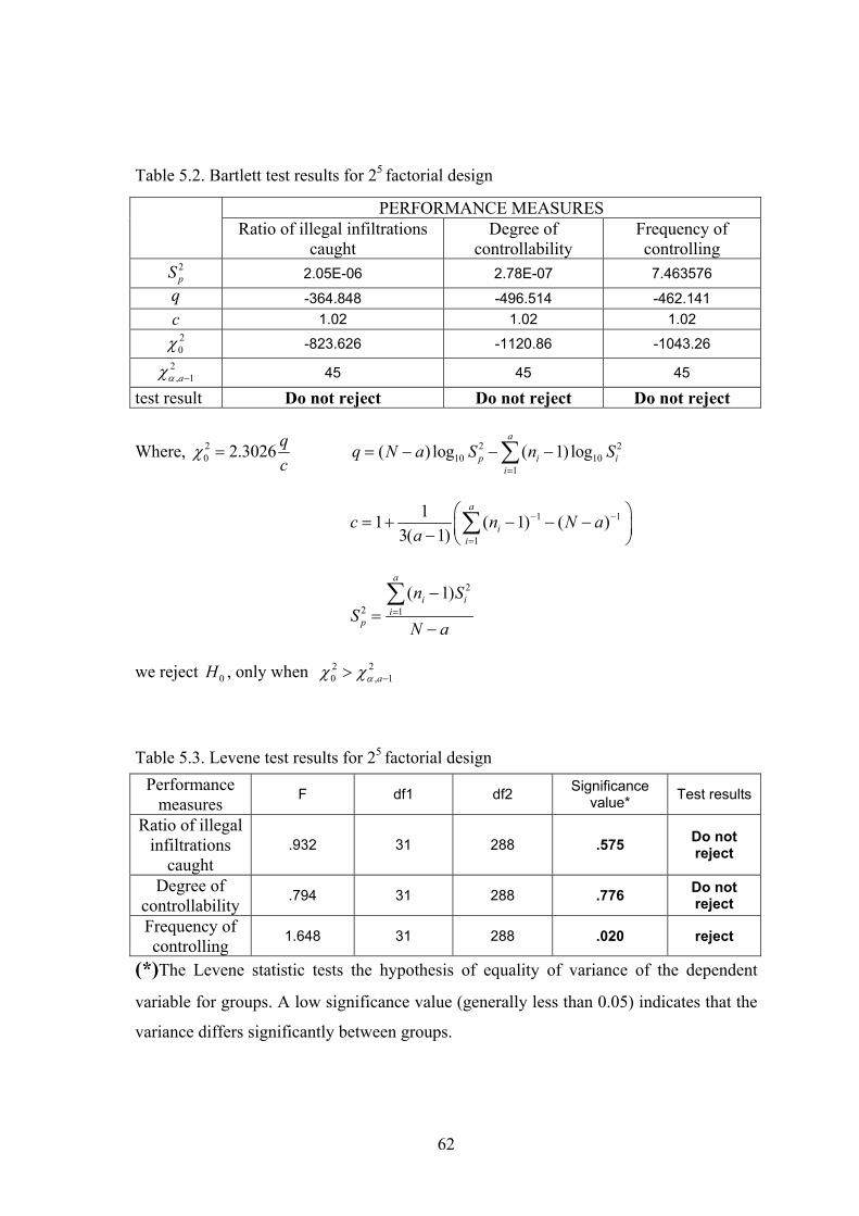
To have a sound statistical analysis, we have to check the homogeneity of

variances and normality assumptions. Thus, we first applied Bartlett test (Montgomery

1992) and Levene test (Levene 1960). As presented in Table 4.6 and Table 4.7,

homogeneity of variances is rejected for each performance measure.

Table 4.6. Levene Test Results

(*)A low significance value (generally less than 0.05) indicates that the variance differs significantly between groups. Table 4.7 Bartlett Test Results

(*) we reject 0H , only when 2 20 , 1aαχ χ −>

When we examine the results in detail (Appendix B, Tables B.1-B.3), we observe that

variance of one of the design points (when there is no security element in the system) for

each performance measure is zero. Since variance stabilization techniques cannot help

due to zero variance data points, we use the results of factorial design as suggestive

rather than conclusive. These diagrams for each performance measure are presented in

Figure 4.11.

Performance measures F df1 df2 Significance

value* Test result

Ratio of Illegal Infiltrations

Caught 2.720 15 144 .001 reject

Degree of Controllability 6.073 15 144 .000 reject

Frequency of Controlling 5.483 15 144 .000 reject

PERFORMANCE MEASURES Ratio of illegal infiltrations caught Degree of controllability Frequency of controlling

2pS 4.17E-05 1.13E-05 93.85977

q 43.8978852 71.08673 79.01167 c 1.04 1.04 1.04

20χ 97.1916061 157.3888 174.9349

2, 1aαχ − 25 25 25

test result Reject* Reject* Reject*

56

By considering these results, we conclude that the most effective factor for

ROIIC is patrols (see Figure 4.11a). Other security elements also improve ROIIC, but not

as much as patrols. In terms of DOC each security element improves DOC (Figure

4.11b). As seen in Figure 4.11c, patrols have positive effect for FOC whereas the others

(ambush, thermal camera and askarad) have negative effects. Because, these security

elements improve DOC. As discussed in detail in Section 4.2.2, FOC is less for the zones

that DOC is at high level.

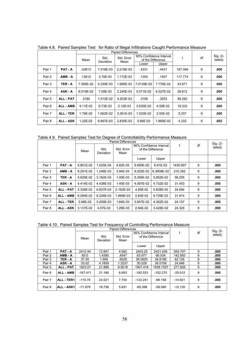
4.3.2. Paired-T Approach

We also apply the paired-T comparison to see if each security element has

statistically impact on the performance measures or not. We use the data given in

Appendix B (Tables B.1-B.3). The paired-T results are presented in Tables 4.8-4.10 for

each performance measure. In these tables, “A” refers to the results of design point that

all factors (security elements) are with their low value (security elements are not in the

system). “All” refers to the results of design point that all factors are with their high

value (all security elements are in the system). “PAT, AMB, TER, ASK” represents

patrols, ambushes, thermal camera and askarad. “Pat-A” is the comparison of when only

patrols are in the system and no security element in the system. “All-Pat” is the

comparison of security elements are in the system and all security elements except

patrols are in the system. All these results indicate that, with their existence in the

system, each security element has significant effect on each performance measure.

57

Main Effects

00.10.20.30.40.50.6

ratio

of i

llega

l inf

iltra

tions

cau

ght

factor a 0.1199025 0.4896465

factor b 0.26312975 0.34641925

factor c 0.285651375 0.323897625

factor d 0.289831625 0.319717375

-1 1

a) Main Effect Diagram (Ratio of illegal infiltrations Caught)

Main Effects

00.040.080.120.160.2

degr

ee o

f con

trolla

bilit

y

factor a 0.0869655 0.148215125

factor b 0.08080625 0.154374375

factor c 0.094042875 0.14113775

factor d 0.098834 0.136346625

-1 1

b) Main Effect Diagram (Degree of Controllability)

Main Effects

0500

10001500200025003000

frequ

ency

of c

ontro

lling

factor a 64.45863125 2227.0885

factor b 1172.9 1118.56525

factor c 1166.720071 1124.82706

factor d 1158.443083 1133.104049

-1 1

c) Main Effect Diagram (Frequency of Controlling)

Figure 4.11 Main effect diagrams of each performance measure

58

Table 4.8. Paired Samples Test for Ratio of Illegal Infiltrations Caught Performance Measure

Table 4.9. Paired Samples Test for Degree of Controllability Performance Measure

Paired Differences 95% Confidence Interval

of the Difference

t

df

Sig. (2-tailed)

Mean

Std. Deviation

Std. Error Mean

Lower Upper

Pair 1 PAT - A 6.901E-02 1.525E-04 4.82E-05 6.890E-02 6.91E-02 1430.907 9 .000

Pair 2 AMB - A 8.291E-02 1.246E-03 3.94E-04 8.202E-02 8.3808E-02 210.392 9 .000

Pair 3 TER - A 5.625E-02 3.162E-03 1.00E-03 5.399E-02 5.852E-02 56.255 9 .000

Pair 4 ASK - A 4.414E-02 4.438E-03 1.40E-03 4.097E-02 4.732E-02 31.453 9 .000

Pair 5 ALL - PAT 5.339E-02 6.837E-03 2.162E-03 4.85E-02 5.828E-02 24.694 9 .000

Pair 6 ALL - AMB 6.284E-02 6.226E-03 1.969E-03 5.83E-02 6.729E-02 31.914 9 .000

Pair 7 ALL - TER 3.98E-02 5.209E-03 1.64E-03 3.607E-02 4.352E-02 24.157 9 .000

Pair 8 ALL - ASK 3.137E-02 4.07E-03 1.28E-03 2.84E-02 3.428E-02 24.329 9 .000

Table 4.10. Paired Samples Test for Frequency of Controlling Performance Measure Paired Differences

95% Confidence Interval of the Difference

t

df

Sig. (2-tailed)

Mean

Std. Deviation

Std. Error Mean

Lower Upper

Pair 1 PAT - A 2412.44 12.847 4.062 2403.25 2421.636 593.797 9 .000 Pair 2 AMB - A 65.0 1.4380 .4547 63.977 66.034 142.950 9 .000 Pair 3 TER - A 37.45 1.906 .6029 36.0920 38.8198 62.126 9 .000 Pair 4 ASK - A 33.02 4.1859 1.3237 30.028 36.0158 24.946 9 .000 Pair 5 ALL - PAT 1923.07 21.888 6.9218 1907.418 1938.7357 277.826 9 .000 Pair 6 ALL - AMB -167.411 21.166 6.693 -182.553 -152.270 -25.012 9 .000

Pair 7 ALL - TER1 -115.70 24.521 7.754 -133.241 -98.158 -14.921 9 .000

Pair 8 ALL - ASK1 -71.978 18.756 5.931 -85.396 -58.560 -12.135 9 .000

Paired Differences 95% Confidence Interval

of the Difference Mean Std. Deviation

Std. Error Mean Lower Upper

t df Sig. (2-tailed)

Pair 1 PAT - A .43813 7.018E-03 2.219E-03 .4331 .4431 197.394 9 .000

Pair 2 AMB - A .13812 3.70E-03 1.172E-03 .1354 .1407 117.774 9 .000

Pair 3 TER - A 7.395E-02 5.330E-03 1.685E-03 7.0139E-02 7.776E-02 43.871 9 .000

Pair 4 ASK - A 6.019E-02 7.09E-03 2.245E-03 5.511E-02 6.527E-02 26.812 9 .000

Pair 5 ALL - PAT .3180 1.013E-02 3.203E-03 .3108 .3253 99.282 9 .000

Pair 6 ALL - AMB 4.11E-02 6.73E-03 2.12E-03 3.635E-02 4.59E-02 19.333 9 .000

Pair 7 ALL - TER 1.79E-02 1.062E-02 3.361E-03 1.033E-02 2.55E-02 5.337 9 .000

Pair 8 ALL - ASK 1.22E-02 8.967E-03 2.835E-03 5.86E-03 1.869E-02 4.332 9 .002

59

CHAPTER 5 Design and Analysis of Experiments

In the previous chapter, we analyzed the system behavior by examining the

relationships between the security elements and the performance measures and

relationships between the performance measures. We also investigated effects of each

security element on each performance measure. Since the security elements have

significant affects, we further examine them for various policies in this chapter.

The degree of use of security elements, stationary or mobile use of security

elements, time period that patrols spend on border control and type of patrols (motorized

or on-foot) are such policies about how security elements are used for protection of

borders. In this chapter, we study for how and how much do such policies affect the

system performances and find out the possible ways of improving performance measures.

5.1. 25 Factorial Design

In Chapter 4.3.1, we have performed 24 factorial design to assess the effect of

each security element (patrols, ambushes, thermal camera and askarad) on the

performance measures. In this chapter, we investigate the effects of different policies on

each performance measure. The policies are (1) the degree of use of high-tech devices,

(2) the degree of use of night-vision tools, (3) stationary or mobile characteristics of duty,

(4) the degree of use of motorized patrols, (5) duty time of patrols. We consider these

policies as factors that affect the system performances, such as ratio-of-illegal-

infiltrations-caught, degree-of-controllability, frequency-of-controlling.

60

We determine these factors and their levels according to Border Services

Instruction (KKY 118-1) and by consulting military experts. All factors are controllable.

It is recommended in Border Services Instruction not to use high-tech devices frequently.

Because, it is desired to extend the lifetime of these devices. Moreover, failure of these

devices is an undesired situation for commanders. Thus, they may prefer to use these

devices seldom. On the other hand, operational activities for protection of borders need

these devices. Above statements are valid for night-vision tools and motorized patrols.

Therefore, we set low and high values of factors a, b and d according to how frequent

these devices are used. The levels of factors indicate the probability of use of the high-

tech devices or night-vision tools for duty of that day. The commander determines

stationary or mobile characteristics of duty. This varies according to number of critical

zones or terrain conditions. The levels of the factor indicate what percent the duty will be

mobile. The maximum time that patrols spent on border control is determined as 4 hours

in Border Services Instruction. But most of the troops apply 3-hour policy. The factors

and their levels are presented in Table 5.1.

Table 5.1. Factors and levels of 25 factorial design

FACTOR FACTOR DESCRIPTION -1 +1

A The degree of use of high-tech devices 40% 95%

B The degree of use of night-vision tools 25% 75%

C Determination of stationary or mobile characteristics of duty

30% 70%

D The degree of use of motorized patrols 15% 70%

E Duty time of patrols 3 hours 4hours

61

We implement 25 factorial design study, which consists of 32 design points. We

investigate the main and interaction effects of factors on each system response. We take

10 simulation runs of each design point, so that the randomization is satisfied to make

factorial design. Results of 25 factorial design for each performance measure are

presented in Appendix C (Table C.3-C.5). To find out the significant factors and their

interactions, we implement analysis of variance (ANOVA).

5.2. Implementation of ANOVA

To implement analysis of variance, two main ANOVA assumptions

(homogeneity of variances and normality) must be satisfied. Because any violation of

ANOVA assumptions may cause serious problems in the final analysis.

Homogeneity of Variances

We test the following hypothesis:

2 2 20 1 2: ......... aH σ σ σ= = =

1H : above not true for at least one 2iσ

We apply Bartlett’s (Montgomery 1992) and Levene’s (Levene 1960) tests. The

results are presented in Tables 5.2-5.3.

62

Table 5.2. Bartlett test results for 25 factorial design

Where, 20 2.3026 q

cχ = 2 2

10 101

( ) log ( 1) loga

p i ii

q N a S n S=

= − − −∑

1 1

1

11 ( 1) ( )3( 1)

a

ii

c n N aa

− −

=

= + − − − − ∑

2

2 1

( 1)a

i ii

p

n SS

N a=

−=

−

∑

we reject 0H , only when 2 20 , 1aαχ χ −>

Table 5.3. Levene test results for 25 factorial design

(*)The Levene statistic tests the hypothesis of equality of variance of the dependent

variable for groups. A low significance value (generally less than 0.05) indicates that the

variance differs significantly between groups.

PERFORMANCE MEASURES Ratio of illegal infiltrations

caught Degree of

controllability Frequency of controlling

2pS 2.05E-06 2.78E-07 7.463576

q -364.848 -496.514 -462.141 c 1.02 1.02 1.02

20χ

-823.626 -1120.86 -1043.26 2

, 1aαχ − 45 45 45

test result Do not reject Do not reject Do not reject

Performance measures F df1 df2 Significance

value* Test results

Ratio of illegal infiltrations

caught .932 31 288 .575 Do not

reject

Degree of controllability .794 31 288 .776 Do not

reject Frequency of controlling 1.648 31 288 .020 reject

63

Bartlett test results in Table 5.2 indicate that homogeneity of variances is satisfied

for each performance measure. But, Levene test results in Table 5.3 indicate that

homogeneity of variances is not satisfied for FOC. To be on the safe side, we decided to

take the suggestion of Levene test (i.e., we accept the results of Levene test). We further

analyze the results of 25 factorial design for FOC presented in Appendix C (Table C.5).

These results indicate that frequency-of-controlling is highly affected by factor d (degree

of use of motorized patrols). We compare the results of design points when factor d is

with its high value and the results of design points when factor d is with its low value by

using t test. The test result is presented in Table 5.4.

Table 5.4. t-test for FOC

As seen in Table 5.4, there is statistically significant difference between two groups of

results. This means that the motorized patrols make big differences in the data set. This

in turn breaks the common variance assumption. Thus we decided to implement two 24

factorial designs instead of 25 for the FOC measure by isolating this factor. When we

apply Bartlett and Levene for 4 factors, we see that homogeneity of variances is satisfied

Levene's Test for Equality of Variances

t-test for Equality of Means

99% Confidence Interval of the

Difference

F

Sig.

t

df

Sig. (2-tailed)

Mean Difference

Std. Error Difference

Lower Upper

3.852 .059 17.22 30 .000 733.803 42.5915 616.676 850.929X Equal variances

assumed

Equal variances not assumed

17.22 25.86 .000 733.803 42.5915 615.40 852.201

64

(see the results in Table 5.5-5.6). Scatter plots given in Appendix D (Figure D.1a-D.1d)

also confirm the common variance assumption.

Table 5.5. Bartlett Test Results For 24 Factorial Design

Table 5.6. Levene Test Results For 24 Factorial Design

Normality Assumptions

A check of the normality assumption can be made by plotting a histogram of

residuals. The residuals for the ith treatment are found by subtracting the treatment

average from each observation in that treatment. Residuals are presented in Appendix D

(Table D.1). If the normality assumption is satisfied, histogram of residuals should look

like a sample from a normal distribution centered at zero. The histogram compared with

normal is presented in Figure 5.1 for the ROIIC performance measure. In Appendix D

(Figure D.2a-D.2c) histograms are presented for other two measures (FOC and DOC). As

seen in these figures, histogram of residuals look like a sample from a normal

F df1 df2 Significance value

Motorized patrol with high level .858 15 144 .611

Motorized patrol with low level 1.228 15 144 .257

Frequency of Controlling Motorized patrol with high level Motorized patrol with low level

2pS 488.3762 227.5717

q 3.95793 9.098046 c 1.04 1.04

20χ 8.763009 20.14342

2, 1aαχ − 25 25

test result Do not reject Do not reject

65

distribution centered at zero. It shows us the normality assumption for each performance

measure is satisfied.

6

5

4

3

2

1

0 N = 31.00

Figure 5.1. Histogram of residuals compared with normal for ratio of illegal infiltrations caught

Another useful procedure is to construct a normal probability plot of residuals. If

the distribution is normal, this plot will resemble a straight line. The normal probability

plot of residuals for ROIIC is presented in Figure 5.2. In Appendix D (Figures D.3a-

D.3c), normal probability plots are presented for FOC and DOC. As seen in these figures,

plots of residuals resemble a straight line. It shows that the normality assumption is

satisfied for each performance measure. Scatter plot of residuals are also presented in

Appendix D (Figures D.4a-D.4d). As seen in these figures, residuals are structureless that

is; normality assumption is satisfied for each performance measure.

66

Observed Cum Prob

1.00.75 .50.250.00

Expected Cum Prob

1.00

.75

.50

.25

0.00

Figure 5.2. Normal P-P of residuals for ratio of illegal infiltrations caught

After satisfying analysis of variance assumptions, we calculate the main and

interaction effects of the factors for each performance measure. The ANOVA test is

implemented by using SPSS statistical package program and the results are presented in

Appendix C (Table C.6-C.10) for each performance measure. Normal probability plot of

main and interaction effects are presented in Appendix C (Table C.11 and Figures C.1a-

C.1d) to validate the ANOVA results (as seen in these figures, all of the insignificant

effects of ANOVA results lie along the zero line, whereas the significant effects are far

from line).

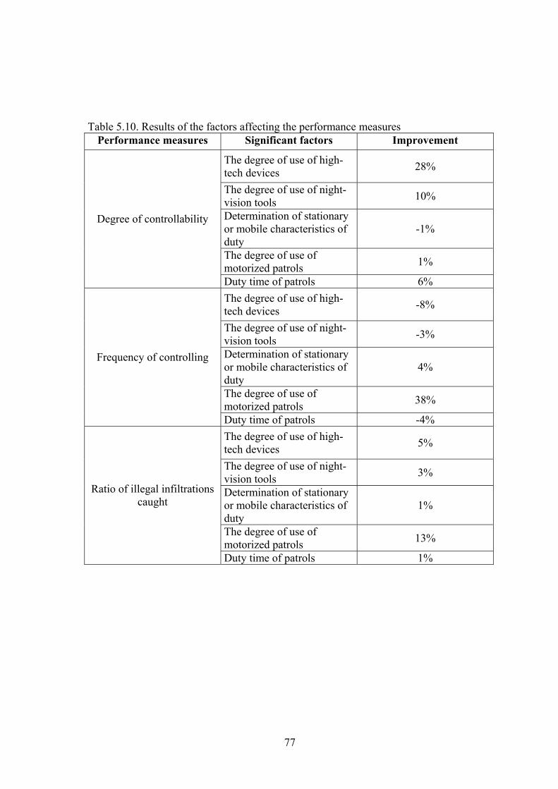
5.3. Interpretation of ANOVA Results of the Performance Measures

In this section, we interpret main and interaction effects of factors for each

performance measure by analyzing the ANOVA results. Recall that our performance

measures are ratio-of-illegal-infiltrations-caught (ROIIC), degree-of-controllability

(DOC) and frequency-of-controlling (FOC).

67

5.3.1. Interpretation of Main Effects and Interactions of Ratio of Illegal

Infiltrations Caught Performance Measure.

The SPSS output of ROIIC statistics is given in Appendix D (Table C.6). It is

clear that each factor is significant. We present the main effect diagram of factors for

ROIIC in Figure 5.3. As seen in this figure, factor d (degree of use of motorized patrols)

has the greatest effect on ROIIC. This is due to increase in the mobility of patrols. When

the motorized type of patrols increase, frequency of controlling the zones increases.

Recall from Chapter 4 (Section 4.2.4.2) that the ROIIC improves as FOC increases. FOC

increases 38% when degree of use of motorized patrols is at its high level as seen in

Figure 5.7. This improvement in FOC increases ROIIC 13% (Figure 5.3). When factor a

(degree of use of high-tech devices) is at high level, DOC increases 28% (Figure 5.5).

Recall from Chapter 4 (Section 4.2.4.1) that ROIIC increases as DOC increases but not

proportionally. The improvement in DOC increases ROIIC 5% (Figure 5.3).

0.50.510.520.530.540.550.560.570.580.590.6

0.610.62

ratio

of i

llega

l inf

iltra

tions

cau

ght

factor a 0.561457318 0.586154383

factor b 0.56637895 0.581232751

factor c 0.571692111 0.57591959

factor d 0.539943338 0.607668363

factor e 0.571994277 0.575617424

-1 1

Figure 5.3. Main effect diagram of factors for ratio of illegal infiltrations caught

68

The graphs in Figure 5.4 are very useful in interpreting significant interactions.

However, they should not be utilized as the sole technique of data analysis because their

interpretation is subjective and their appearance is often misleading (Montgomery 1992).

Therefore, in addition to these graphs, we construct Tables 5.7-5.9 for each performance

measure.

There are four significant interactions on ROIIC. These are between factors a-d,

b-d, e-d and a-b-d-e. Notice that interactions are between factors (a, b and e) that have

positive effect on DOC and factor (d) that has positive effect on FOC (explanation is

given in Sections 5.3.2 and 5.3.3. The interactions between factors are presented in

Figure 5.4a-5.4d. In these figures, the two lines are parallel to each other that indicate a

lack of interaction. Thus, we explain interactions by using results in Table 5.7. There is

an interaction between factors a and d since the effect of factor d on ROIIC depends on

the level chosen for factor a. When the degree of use of high-tech devices is high, longer

time the zones will be under control and this will decrease the control of zones by patrols

(as explained in Chapter 4.2.2). When the degree of use of high-tech devices is low, less

time the zones will be under control and this will increase the control of zones by patrols.

Thus, effect of factor d on ROIIC will be less when factor a is with its high value and

effect of factor d on ROIIC will be more when factor a is with its low value. Interactions

b-d and e-d can be explained by same reasoning since factors b and e are like factor a

(factors that increase DOC) and the second factor in the interactions is factor d same as in

interaction a-d. The last interaction, abde, consists of factors that are in the two-

interactions. As seen in Table 5.7 (four interaction), when the three factors (a, b, e) are

with their high levels, the effect of factor d on ROIIC is less and when the three factors

(a, b, e) are with their low levels, the effect of factor d on ROIIC is more.

69

Table 5.7. Interactions between factors for ROIIC

Interactions Ratio of Illegal Infiltrations Caught

D

high low difference high 0.6185 0.5537 0.0648 low 0.5967 0.5261 0.0706

AD A

difference 0.0218 0.0276 D

high low difference

high 0.6137 0.5487 0.065 low 0.6016 0.0705 0.0705

BD B


high low difference

high 0.6081 0.5427 0.0654 low 0.6068 0.5371 0.0697

ED E


high low difference

high 0.6260 0.5876 0.0384 low 0.5634 0.5149 0.048

ABDE ABE

difference 0.0625 0.0726

70

AD interaction

0.51

0.53

0.55

0.57

0.59

0.61

-1 1factor d

ratio

of i

llega

l in

filtra

tions

cau

ght

factor a low levelfactor a high level

a) Interaction between factor a and d BD interaction

0.48

0.5

0.52

0.54

0.56

0.58

0.6

0.62

-1 1factor d

ratio

of i

llega

l inf

iltra

tions

ca

ught

factor b low level

factor b high level

b) Interaction between factor b and d ED interaction

0.5

0.52

0.54

0.56

0.58

0.6

0.62

-1 1factor d

ratio

of i

llega

l in

filtra

tions

cau

ght

factor elow levelfactor ehigh level

c) Interaction between factor e and d

ABDE interaction

0.50.520.540.560.580.6

0.620.64

-1 1factor d

ratio

of i

llega

l in

filtra

tions

cau

ght

factor abe low levelfactor abe high level

d) Interaction between factor a,b,e and d Figure 5.4. Interactions between factors

71

5.3.2. Interpretation of Main Effects and Interactions of Degree of

Controllability Performance Measure

The SPSS output of DOC statistics is given in Appendix D (Table C.7). The

results indicate that each factor is significant. As seen in Figure 5.5, factor a (degree of

use of high-tech devices) has the greatest effect on DOC. This is due to usage of high-

tech devices more frequently. When degree of use of high-tech devices is high, longer

time the zones are under control. Then, DOC increases 28% when degree of use of high-

tech devices is at high level as seen in Figure 5.5.

0.2

0.21

0.22

0.23

0.24

0.25

0.26

0.27

0.28

degr

ee o

f con

trolla

bilit

y

factor a 0.212489856 0.272734808

factor b 0.231557816 0.253666849

factor c 0.244487654 0.24073701

factor d 0.241908541 0.243316124

factor e 0.235839083 0.249385581

-1 1

Figure 5.5. Main effect diagram of factors for degree of controllability

There are two significant interactions on DOC. These are between factors a-b and

a-e. Notice that interactions are between factors that have all positive effect on DOC. The

interactions between factors are presented in Figure 5.6a-5.6b and Table 5.8. There is an

interaction between a and b since the effect of factor b on DOC depends on the level

chosen for factor a. When the degree of use of high-tech devices is high, longer time the

72

zones will be under control and this will increase the probability of taking the same zones

under control by ambushes and patrols. Thus, effect of factor b on DOC will be less

when factor a is with its high value and effect of factor b on DOC will be more when

factor a is with its low value. Interaction a-e can be explained by same reasoning since

factor e is like factor b (factors that increase DOC) and the second factor in the

interaction is factor a same as in interaction a-b.

AB interaction

0.20.210.220.230.240.250.260.270.280.29

-1 1factor b

degr

ee o

f con

trolla

bilit

y

factor alow levelfactor ahigh level

AE interaction

0.20.210.220.230.240.250.260.270.280.29

-1 1factor e

degr

ee o

f con

trolla

bilit

y

factor alow level

factor ahigh level

a) Interaction between factor a and b b) Interaction between factor a and e Figure 5.6. Interactions between factors Table 5.8. Interactions between factors for degree of controllability

Interaction Degree Of Controllability

B

high low difference high 0.2829 0.2625 0.0204 low 0.2244 0.2005 0.0239

AB A

difference 0.0585 0.062 E

high low difference

high 0.2788 0.2199 0.0589 low 0.2666 0.2050 0.0616

AE A

difference 0.0122 0.0149

73

5.3.3. Interpretation of Main Effects and Interactions of Frequency of

Controlling Performance Measure

The SPSS output of FOC statistics is given in Appendix D (Table C.8-C10). The

results indicate that each factor is significant. As seen in Figure 5.3, factor d (degree of

use of motorized patrols) has the greatest effect on FOC. This is due to increase in the

mobility of patrols. When the degree of use of motorized patrols is high, frequency of

controlling the zones increases. FOC increases 38% when degree of use of motorized

patrols is at high level as seen in Figure 5.5.

1500

1700

1900

2100

2300

2500

2700

2900

frequ

ency

of c

ontro

lling

factor a 2391.164658 2204.775819

factor b 2328.587128 2267.353348

factor c 2259.73378 2336.206696

factor d 1931.06875 2664.871726

factor e 2340.073363 2255.867113

-1 1

Figure 5.7. Main effect diagram of factors for frequency of controlling

We divided 25 factorial design into two 24 factorial designs as we discussed in the

homogeneity of variances section (Section 5.2). As seen in Figures 5.7a-5.7b both 24

factorial design main effect graphs are similar. Factor c (stationary or mobile

characteristics of duty) has the greatest effect on FOC. This is due to increase in the

74

1750

1800

1850

1900

1950

2000

2050

frequ

ency

of c

ontro

lling

factor a 2001.120536 1861.016964

factor b 1954.119941 1908.01756

factor c 1891.947024 1970.190476

factor e 1965.037649 1897.099851

-1 1

a) Main effect diagram of factors for frequency of controlling (factor d is with its low value)

2400

2500

2600

2700

2800

frequ

ency

of c

ontro

lling

factor a 2781.20878 2548.534673

factor b 2703.054315 2626.689137

factor c 2627.520536 2702.222917

factor e 2715.109077 2614.634375

-1 1

b) Main effect diagram of factors for frequency of controlling (factor d is with its high value)

Figure 5.8. Main effect diagram of factors for frequency of controlling

75

mobile duties. When mobile duties increase, frequency of controlling the zones increases.

FOC increases 4% when factor c is with its high level. Factors a, b and e have negative

effect on FOC. This is due to increase in the DOC. These factors improve DOC, since

longer time the zones will be under control when they are with their high levels. Recall

from Chapter 4.2.2 that FOC is less for the zones that DOC is at high level.

There are four significant interactions on FOC. These are between factors a-c, a-

b, b-c and b-e. The interactions between factors are presented in Figure 5.9a-5.9d and

Table 5.9. Interactions between factors a-b and b-e are between factors that have positive

effect on DOC. These interactions can be interpreted as the ones in Section 5.3.2.

Interactions between factors a-c and b-c are between factors (a, b) that have positive

effect on DOC and factor (c) that has positive effect on FOC. These interactions can be

interpreted as the ones in Section 5.3.1.

Table 5.9. Interactions between factors for frequency of controlling

Interactions Frequency of controlling

B

high low difference high 2515 2582 -67 low 2738 2824 -86

AB A

difference -223 -242 B

high low difference

high 2671 2732 -61 low 2581 2673 -92

BC C

difference 90 59 B

high low difference

high 2571 2657 -86 low 2681 2748 -67

BE E

difference -110 -91 A

high low difference

high 1905 2034 -129 low 1816 1967 -151

AC C

difference 89 67

76

AB interaction

2300

2400

2500

2600

2700

2800

2900

-1 1factor b

frequ

ency

of c

ontro

lling

factor alow level

factor ahighlevel

AC interaction

170017501800185019001950200020502100

-1 1factor a

freq

uenc

y of

con

trollin

g

factor clow level

factor chigh level

a) Interaction between factors a and c b) Interaction between factors a and b

BC interaction

2500

2550

2600

2650

2700

2750

-1 1factor b

frequ

ency

of c

ontro

lling

factor clowlevelfactorchighlevel

BE interaction

24502500255026002650270027502800

-1 1factor b

frequ

ency

of c

ontro

lling

factor dlow level

factor dhighle el

c) Interaction between factors b and c d) Interaction between factors b and e Figure 5.8 Interactions between factors

All these results are summarized in Table 5.10. Specifically, the magnitude and

the direction of the factor effects on each performance are given in this table. Note that

the effects of the factors are measured when we change the level of the factors from its

low level to high level.

77

Table 5.10. Results of the factors affecting the performance measures

Performance measures Significant factors Improvement

The degree of use of high-tech devices 28%

The degree of use of night-vision tools 10%

Determination of stationary or mobile characteristics of duty

-1%

The degree of use of motorized patrols 1%


Duty time of patrols 6% The degree of use of high-tech devices -8%

The degree of use of night-vision tools -3%


4%



Duty time of patrols -4% The degree of use of high-tech devices 5%

The degree of use of night-vision tools 3%


1%



Duty time of patrols 1%

78

In concluding this chapter, we observe that factor d (degree of use of motorized

patrols) has the greatest effect on ROIIC. FOC increases 38% when degree of use of

motorized patrols is at its high level. This improvement in FOC increases ROIIC 13%.

The factor a (degree of use of high-tech devices) follows factor d in the significance.

When factor a is at high level, DOC increases 28%. This improvement in DOC increases

ROIIC 5%. The factor b (The degree of use of night-vision tools) increases DOC 10%

and ROIIC 3%. When factor e (duty time of patrols) is at high level DOC increases 6%

but improvement in ROIIC is only 1%. Other factors (degree of use of motorized patrols

and determination of stationary or mobile characteristics of duty) have little effect on

DOC. The factors a,b and e have negative effects on FOC.

There are mainly two kinds of interaction. These are: (1) interaction between

factors that have positive effect on DOC (factors a,b,e) and factors that have positive

effect on FOC (c,d) such as a-c, b-d, a-d. When a,b,e is high, longer time the zones will

be under control and this prevents the occurrence of control of zones different times. (2)

interaction between factors that have positive effect on DOC such as a-b, b-e. When one

of these factors is high, longer time the zones will be under control and this will increase

the probability of taking the same zones under control by security elements.

Commanders have to know that, when they increase the levels of more than one

factor, the effect on performance measure will be less than total effect of each factor. For

example, factor a improves ROIIC 5% and factor d improves 13%. When both factor are

at high level, ROIIC increases 16% (note that it is 18% when we add effects of each

factor).

79

CHAPTER 6

Alternatives and Border Security System Model in the Support of

Decision-making Process

In Chapters 4 and 5, we have analyzed the system behavior, investigated effect of

each security element on the performance measures and identified the significant factors.

In this chapter, we develop different alternatives. These alternatives are the possible

improvement methods. We know that improvement border security will cause financial

costs. We evaluate these alternatives, compare and rank them by using ranking/ selection

and multi-criteria decision-making procedures. The criteria are again our performance

measures degree-of-controllability (DOC), frequency-of-controlling (FOC), ratio-of-

illegal-infiltrations-caught (ROIIC) and cost.

Specifically, we will attempt to answer the following research questions:

• If coordination is established between security elements, how much does

it affect the performance measures?

• How much do additional high-tech devices affect the performance

measures?

• Which improvement method is the best considering different criteria?

• What is the effect of high mobility of patrols on the system

performances?

80

6.1. Alternatives

1. Benchmark system: It is the existing system and this is included in comparisons

to observe the effect of coordinated system.

2. The border security system that all patrols are motorized: When we analyzed

the system in the previous chapters, we observed that the ROIIC increases as FOC

increases. We also observed that FOC increases as motorized type of patrols increases.

By including this improvement method, we will observe the effect of high mobility of

patrols on the system performances.

3. The system one more askarad and one more thermal camera added: These

high-tech devices make it possible to control wider borderline. We know that ROIIC

increases as DOC increases. We include this improvement method to observe the effect

of additional high-tech devices.

4. The system with coordinated security elements: In the system, sometimes

overlaps occur since the security elements take control the same zones. We prevent these

overlaps by making it possible to have better coordination between security elements. As

a result, we expect the DOC performance measure increases.

5. The system with coordination established and all patrols are motorized: This

is the combination of the second and forth alternatives.

6. The system with coordination and one more askarad and thermal camera

added: Specifically, by including this alternative, we try to observe the effect of

coordination when high-tech devices are increased. We expect that the degree-of-

controllability increase.

81

6.2. Evaluation of Alternatives by Using Ranking and Selection

Procedures.

6.2.1. All Pairwise Comparisons

We first run the simulation model for each alternative design and obtain the

results. The results for each alternative design are presented in Appendix E (Tables E.1-

E.3) for each performance measure. Then, we make all pairwise comparisons to evaluate

the alternatives. The results of all pairwise comparisons for the ROIIC performance

measure are presented in Table 6.1. The results of all pairwise comparisons for DOC and

FOC are presented in Appendix E (Tables E.4-E.5). We have 6 alternatives and 15

comparisons. We make each comparison with 99% degree of confidence interval. In

Figure 6.1, the pairwise comparisons of alternatives and ranking of alternatives for

ROIIC is presented. In this figure, arrows between alternatives display the comparison of

two alternatives. If the alternative is at the beginning point of arrow, this alternative is

better than the one that is at the end point of arrow. We draw these graphs for all

performance measures and rank the alternatives according to their position either at the

beginning or end point of the arrow. In Figures 6.2 and 6.3, the graph of comparisons and

ranking of alternatives for DOC and FOC are presented.

82

Table 6.1. Paired Samples Test of alternatives for ratio of illegal infiltrations caught

Paired Differences


Difference

t

df

Sig. (2-tailed)

Mean

Std. Deviation

Std. Error Mean

Lower Upper

Pair 1 ALT1 - ALT2 -.101083 1.57E-02 4.96E-03 -.117219 -8.49E-02 -20.359 9 .000

Pair 2 ALT1 - ALT3 -3.00E-02 1.09E-02 3.47E-03 -4.13E-02 -1.87E-02 -8.651 9 .000

Pair 3 ALT1 - ALT4 -5.97E-03 1.06E-02 3.37E-03 -1.69E-02 4.99E-03 -1.771 9 .110

Pair 4 ALT1 - ALT5 -.104150 1.04E-02 3.31E-03 -.114933 -9.33E-02 -31.388 9 .000


Pair 6 ALT2 - ALT3 7.10E-02 1.33E-02 4.22E-03 5.73E-02 8.47E-02 16.803 9 .000

Pair 7 ALT2 - ALT4 9.51E-02 1.23E-02 3.90E-03 8.24E-02 .1077962 24.363 9 .000

Pair 8 ALT2 - ALT5 -3.06E-03 1.34E-02 4.25E-03 -1.68E-02 1.07E-02 -.722 9 .489





Pair 13 ALT4 - ALT5 -9.81E-02 1.07E-02 3.39E-03 -.109201 -8.71E-02 -28.939 9 .000



83

Ranking Alternatives 1 Alt 2≅ Alt 5 2 Alt 6 3 Alt 3 4 Alt 1≅ Alt 4

Figure 6.1. The pairwise comparisons of alternatives and ranking of alternatives for ratio of illegal infiltrations caught performance measure

Ranking Alternatives 1 Alt 6 2 Alt 3 3 Alt 5 4 Alt 1≅ Alt 2≅ Alt 4

Figure 6.2.The pairwise comparisons of alternatives and ranking of alternatives for DOC

Alt1

Alt3

Alt2 Alt4

Alt5

Alt6

Alt1

Alt3

Alt2 Alt4

Alt5

Alt6

84

Ranking Alternatives

1 Alt 2≅ Alt 5 2 Alt 1≅ Alt 4 3 Alt 3≅ Alt 6

Figure 6.3. The pairwise comparisons of alternatives and ranking of alternatives for FOC As seen in Figures 6.1-6.3, the second and the fifth alternatives are better than

others for ROIIC and FOC. Alternative 6 and alternative 3 are in the second and third

row for ROIIC, respectively. But they are the last for FOC. On the other hand, sixth

alternative is the best and third alternative is the second for DOC. This shows that

ranking of alternatives are not consistent for each performance measure.

We observe that when resources are increased coordination gets importance for

both DOC and ROIIC. Because, the sixth alternative is better than the third alternative

for both performance measures.

Alt1

Alt3

Alt2 Alt4

Alt5

Alt6

85

6.2.2. Rinott’s Procedure

Although we made all pairwise comparisons, we couldn’t rank the alternatives to

find the best alternative. Then, we apply Rinott’s ranking and selection procedure (1978).

We first find the required number of replications for each alternative. The required

numbers of replications are presented with results of alternatives in Appendix E (Tables

E.1-E.3). Then we calculate the average of replications and select the alternative with the

highest average as the best one.

In our study, we take h10, 0.05 = 3.859 and indifference amount value (d) for the

ROIIC and DOC performance measures 0.005 whereas 10 for the FOC performance

measure. The rankings of alternatives for each performance measure are presented in

Tables 6.2-6.4.

Tables 6.2. Ranking of alternatives for ratio of illegal infiltrations caught

Table 6.3. Ranking of alternatives for degree of controllability

Ranking Alternatives Values 1 Alternative 5 0.634905 2 Alternative 2 0.631838 3 Alternative 6 0.571622 4 Alternative 3 0.560787 5 Alternative 4 0.536729 6 Alternative 1 0.530754


86

Table 6.4. Ranking of alternatives for frequency of controlling

As seen in Tables 6.2-6.4, alternative 6 is the best for DOC and alternative 3

follows it. But, alternative 6 is the last for FOC. Alternative 5 is the best for ROIIC and

alternative 2 follows it. On the other hand, second alternative is the best for FOC and the

fifth alternative follows it. All these results indicate that ranking of alternatives are not

consistent for each performance measure.

We also observe that coordination is important to increase performance measures

for both the DOC and ROIIC performance measures. Because, alternative 4 is better than

alternative 1 and alternative 6 is better than alternative 3 for both ROIIC and DOC.

In both ranking and selection procedures, we observe that the ranking of

alternatives are not consistent for each performance measure. Moreover, we have one

more criterion that will effect the decision beyond the performance measures; cost of

alternatives. Thus, we decide to apply multi-criteria decision-making procedures.

Ranking Alternatives Values 1 Alternative 2 3153 2 Alternative 5 3146 3 Alternative 1 2046 4 Alternative 4 2045 5 Alternative 3 1877 6 Alternative 6 1865

87

6.3. Implementation of Geometric Mean Technique for our

Multi-criteria Decision-making Problem

We decide to implement geometric mean technique to our multi-criteria decision-

making problem. Although there are many multi-criteria decision-making methods in the

literature, we choose geometric mean technique. The geometric mean is the way to solve

pairwise comparison matrices. Barzilai, et al. (1987) identified desired properties of this

solution technique. We use geometric mean technique suggested by H.A. Eiselt (course

handouts in Bilkent University 2001)

In the first step we construct our hierarchy tree as seen in Figure 6.5.

Goal: Rank the alternatives Criteria: Ratio of illegal Degree of Frequency of Cost infiltrations caught controllability controlling Alternatives: 1 2 3 4 5 6 1 2 3 4 5 6 1 2 3 4 5 6 1 2 3 4 5 6 Figure 6.4. Hierarchy tree of alternatives and criteria

In the second step, the pairwise comparisons of alternatives are made for each

criterion. Therefore, we construct our pairwise comparison matrices. In this step, since

we know the border security system simulation results for each alternative, we can easily

compare alternatives with each other for any criterion only by determining how much

important the difference between the lowest and the highest score of alternatives. After

consulting military experts, we give importance degree 5 “essentially more important”

for the difference between the alternative with the lowest score and the alternative with

88

the highest score. Then, we make pairwise comparisons of alternatives and we construct

matrices according to values of simulation results. In Table 6.5, results of each

alternative for each criterion are presented. The matrices that show the pairwise

comparisons of alternatives are in Appendix E (Tables E.6a-E.6d).

Table 6.5. Results of each alternative for each criterion

(*) Costs of alternatives are calculated as million $ for one-year time period (note that costs are calculated according to price of thermal camera (0.13 million $), price of askarad (0.24 million $) and amount of fuel needed for motorized patrols.)

In the third step, we construct pairwise comparison matrix for the criterions. We

have four criterions, so we construct four by four pairwise comparison matrix. In this

step, we consulted military experts for pairwise comparisons of criteria. The pairwise

comparisons of criteria are presented in Table 6.6.

Table 6.6. Pairwise comparison matrix of criteria

criteria

alternatives

Ratio of illegal infiltrations

caught



Cost*

1 0.53075 0.21961 2046.64 0.04

2 0.63184 0.22183 3153.56 0.055

3 0.56079 0.2845 1877.88 0.075

4 0.53673 0.2239 2045.77 0.04

5 0.63491 0.22602 3146.43 0.055

6 0.57162 0.29256 1865.71 0.075

Criteria Ratio of illegal

infiltrations caught


Frequency of controlling cost

Ratio of illegal infiltrations caught 1.0000 2.5000 2.2500 1.2500

Degree of controllability 0.4000 1.0000 0.8600 0.4500

Frequency of controlling 0.4444 1.1628 1.0000 0.6000

cost 0.8000 2.2222 1.6667 1.0000

89

In the fourth step, we construct the utility matrix by taking geometric means of each

row of matrices that we construct in the second step. For example, we calculate the

geometric mean of first row of ROIIC matrix (Table E.6a in Appendix E) as 0.426605

and place it first row and first column of utility matrix and we calculate the geometric

mean of second row of ROIIC matrix as 2.50834 and place it second row and first

column of utility matrix. Meanwhile, we construct weight matrix by taking the geometric

means of each row of pairwise comparison matrix of criteria and normalizing the results.

In Tables 6.7-6.8 utility matrix and weight matrix (before and after normalization) are

presented.

Table 6.7. Utility matrix

Alternatives Ratio of illegal




1 0.426605 0.534898 0.703763 2.369284 2 2.50834 0.579024 2.806936 1.077307 3 0.766993 2.520356 0.509854 0.391552 4 0.480913 0.625656 0.703144 2.370273 5 2.603455 0.675191 2.798679 1.077937 6 0.973224 3.032556 0.504556 0.391617

Table 6.8. Weight matrix

In the fifth and the last step, we take the weight powers of each alternative row in

the utility matrix and calculate values of each alternative. Then, we normalize the values.

Ratio of illegal




Weights before normalization 1.628389 0.627253 0.746204 1.311996

Weights after normalization 0.37748 0.145405 0.172979 0.304136

90

The mathematical expression of calculation for alternative 1 is as follow:

V(alt1)= 0.4266050,37748 x 0.5348980,145405 x 0.7037630,172979 x 2.3692840,304136 = 0,809794

Values of each alternative are presented in Table 6.9 and ranking of alternatives is

presented in Table 6.10.

Table 6.9. Values of alternatives Table 6.10. Ranking of alternatives

As seen in Table 6.10, alternative 5 is the best alternative. It shows us the

importance of motorized type of patrols and coordination between security elements in

the system. We also see the importance of coordination by observing alternative 4 in the

third row of ranking. On the other hand, alternatives that need additional high-tech

devices (alternatives 6 and 3) are not preferred because of their high costs. But, if new

high-tech devices are added to the system, coordination must be established between

security elements.

Before

normalization After

normalization

V(alt1) 0.809794 0.126509 V(alt2) 1.59818 0.249674 V(alt3) 0.69252 0.108188 V(alt4) 0.866771 0.13541 V(alt5) 1.65686 0.258841 V(alt6) 0.776948 0.121378


91

CHAPTER 7 Conclusion

7.1. Summary

In this thesis, we give brief information about how Turkey protects and control

her land borders (border security system in Turkey). We first present a literature survey.

Then, we define necessary components of the system and their interactions, which are all

needed to develop a simulation model of border security system. We present our

objectives to perform such a study and model development of the system. Our main aim

is to find out possible ways of increasing border control and security along the land

borders of Turkey. Therefore, we try to: (1) understand the behavior of the system, (2)

observe the relationships between security elements and performance measures and

relationships between performance measures, (3) find-out effect of each security element

on the performance measures, (4) analyze factors that effect the performance measures,

(5) investigate system responses, when changes made in the system or new resources

added to the system, (6) evaluate different alternatives which improve the performance

measures, by using ranking-selection and multi-criteria decision-making procedures. We

try to achieve our objectives by modeling and analysis of operational activities of typical

Border Company supported by Border Battalion via simulation. We analyze the outputs

by using performance measures: (1) ratio-of-illegal-infiltrations-caught, (2) degree-of-

controllability, (3) frequency-of-controlling.

92

7.2. Conclusions and Future Research Directions

1. The behavior of the system in terms of DOC, FOC and ROIIC are not uniform

along the border. This is due to different use of security elements in different

zones and different mobility characteristics of security elements. We can adjust

DOC by using flexible use of security elements. It gives us the opportunity to

control some part of our borders (critical zones) at high level. Ambushes are the

most appropriate resource for controlling critical zones at high level. Therefore,

training of ambushes must be given importance.

2. Patrols are the main security element for frequency of controlling the zones.

Therefore, precautions for increasing the mobility of patrols must be taken (i.e.,

increasing the number of motorized patrols).

3. It is difficult to catch enemy special forces and terrorist type of infiltrations. To

increase catching probability of these infiltrations, importance should be given to

build physical obstacles along the borders. These obstacles increase infiltration

time; so probability of catching illegal infiltrations increases.

4. There is a direct relation between DOC and ROIIC. But, ROIIC does not improve

proportionally with DOC; that is by increasing the quantity of high-tech devices

we don’t necessarily prevent infiltrations on the borderlines. We know that

increasing DOC needs more high-tech devices and this causes increase in the cost

of border security. Therefore, appropriate quantity of high-tech devices must be

identified for each border troop and ambushes must be used for controlling zones

that cannot be controlled by high-tech devices.

5. There is also a direct relation between FOC and ROIIC. But, ROIIC does not

improve proportionally with FOC. Therefore, border security planners must

93

identify the appropriate capacity of patrol and precautions such as increasing the

mobility of patrols and building of physical obstacles must be taken to maximize

ROIIC. Such precautions also deter the infiltrations along the border.

6. Each of security element (patrols, ambushes, thermal camera, askarad) has

statistically significant effect on each performance measure with its existence

when compared to its absence in the system.

7. We analyze the factors that affect the performance measures. All factors have

significant effects on each of the performance measures. In Table 7.1, a summary

is presented. In Table 7.2, factors and their descriptions are given.

Table 7.1 Factors affecting the performance measures.

(*) improvement indicates the change in performance measure when we change the

factor from its low level to high level.

Table 7.2 Factors and their descriptions

Performance Measures Significant Factors Improvement*


A, B, C, D, E 5%, 3%, 1%, 13%, 1%

Degree of controllability A, B, C, D, E 28%, 10%, -1%, 1%, 6%

Frequency of controlling A, B, C, D, E -8%, -3%, 4%, 38%, -4%

Factor Factor Description A The degree of use of high-tech devices

B The degree of use of night-vision tools

C Determination of stationary or moving characteristics of duty

D The degree of use of motorized patrols

E Duty time of patrols

94

According to these results, border troops have to use high-tech devices more

frequently, increase the duty time of patrols, and increase mobility of all security

elements along the borders to increase the security of land borders.

8. Another way of increasing border security is to establish coordination between

security elements. Coordination increases degree of controllability by preventing

control of same zones by two or more security elements at the same time.

9. We evaluate different alternatives by using ranking, selection and multi-criteria

decision-making procedures to give an idea about how border security system

simulation model supports the decision-making process before conducting real

decisions. Alternative description and ranking of alternatives are presented in

Table 7.3.

Table 7.3. Alternative description and ranking of alternatives Ranking Alternative Alternative description Value

1 Alternative 5

System that coordination is established and all patrols are motorized 0.258841

2 Alternative 2

System that all patrols are motorized 0.249674

3 Alternative 4

System that coordination is established between security elements 0.13541

4 Alternative 1

Benchmark system 0.126509

5 Alternative 6

System that coordination is established and one more askarad and one more thermal camera added 0.121378

6 Alternative 3

System with one more askarad and one more thermal camera 0.108188

When we look at the results, alternative 5 (system that coordination is established

and all patrols are motorized) is preferred to other alternatives when we consider

criterions: ratio-of-illegal-infiltrations-caught, degree-of-controllability, frequency-of-

controlling and cost.

95

10. We know that additional security elements cause an increase in the cost of

security of borders. On the other hand, like almost all countries in the world,

we try to control our land borders at high level with limited resources.

Therefore, before conducting real investments or changes to increase border

security, we have to analyze utilities of additional resources or changes in the

system in terms of performance measures and their costs for each border

troop. Thus, the requirements of each border troop are evaluated more

accurately and investments are made more useful.

Future Research Directions

Although the main task of border troops is protection and security of borders in

their responsibility terrain, they have another tasks. They also perform some activities

that support execution of their tasks. Furthermore, operational activities for control and

security of borders may be analyzed under different conditions. Followings are the some

topics that can be investigated by future studies.

1. Border security can be analyzed under situation of any strained relation with

neighbor country before war, by considering the troops located very near to

borders.

2. In our study, we analyze border security system under night conditions. The

system can be analyzed under day conditions or under both night and day

conditions.

3. One of the main tasks of border troops is collection of intelligence by close

watching the terrain of neighbor country. The research can be conducted on

this task of border troops.

96

4. We know that border troops are located in such a way that they execute their

tasks best under peace and war conditions. But, by considering the

developing technology and change in the regional threats, the locations of

border troops at all levels can be analyzed.

5. Logistic activities of border troops can be analyzed.

6. Communication systems of border troops can be analyzed.

97

APPENDIX A Confidence Intervals Table A.1a. Confidence interval for degree of controllability of Border Company

Average Std.Dev. Var Max C.I for degree of controllability of Border

Company 0.219926 0.003599 1.2x10-5 0.22536

C.I low 0.218355 Min Median C.I with α = 0.1 C.I high 0.221496 0.214400 0.219491 C.I low 0.217843 # of reps

C.I. with α = 0.05 C.I high 0.222008 10 C.I low 0.216716

C.I. withα = 0.01 C.I high 0.223135

Table A.1b. Confidence interval for frequency of controlling of Border Company

Average Std.Dev. Var Max C.I for frequency of controlling of Border

Company 2025 8.63111 74.496 2036.583

C.I low 2021.23 Min Median C.I with α = 0.1 C.I high 2028.76 2008.036 2025.595 C.I low 2020.005 # of reps C.I. with α = 0.05 C.I high 2029.99 10 C.I low 2017.303 C.I. withα = 0.01 C.I high 2032.696

Table A.1c. Confidence interval for ratio of ill. inf. caught of Border Company

Average Std.Dev. Var Max C.I for ratio of ill. inf. caught of Border Company 0.530754 0.009157 8.38x10-5 0.5402


98

Table A.2a. Confidence interval for degree of controllability of Border Company

Table A.2b. Confidence interval for frequency of controlling of Border Company

Table A.2c. Confidence interval for ratio of ill. inf. caught of Border Company

Average Std.Dev. Var Max C.I for degree of controllability of Border

Company 0.219926 0.081316 0.006612 0.40744

C.I low 0.184440 Min Median C.I with α = 0.1 C.I high 0.255411 0.04871 0.19374 C.I low 0.17228 C.I. with α = 0.05 C.I high 0.2669 C.I low 0.1474 C.I. withα = 0.01 C.I high 0.2924

Average Std.Dev. Var Max C.I for frequency of controlling of Border

Company 2025 668.71 447177.55 3021.2

C.I low 1733 Min Median C.I with α = 0.1 C.I high 2316 782.4 2003.7 C.I low 1638 C.I. with α = 0.05 C.I high 2411 C.I low 1428 C.I. withα = 0.01 C.I high 2621

Average Std.Dev. Var Max C.I for ratio of ill. inf. caught of Border Company 0.5307 0.129745 0.01683 0.7509


99

Table A.3a. Confidence interval for degree of controllability of 1st Border Platoon

Average Std.Dev. Var Max C.I for degree of controllability of 1st Border

Platoon 0.228424 0.004328 1.88x10-5 0.234066


Table A.3b. Confidence interval for degree of controllability of 2nd Border Platoon

Average Std.Dev. Var Max C.I for degree of controllability of 2nd Border

Platoon 0.206546 0.007785 6.06x10-5 0.215041


Table A.3c. Confidence interval for degree of controllability of 3rd Border Platoon

Average Std.Dev. Var Max C.I for degree of controllability of 3rd Border

Platoon 0.204612 0.012994 0.000168857 0.231256


Table A.3d. Confidence interval for degree of controllability of 4th Border Platoon

Average Std.Dev. Var Max C.I for degree of controllability of 4th Border

Platoon 0.230055 0.007673 5.88x10-5 0.240085


100

Table A.4a. Confidence interval for frequency of controlling of 1st Border Platoon

Average Std.Dev. Var Max C.I for frequency of controlling of 1st Border

Platoon 2551.704 24.56574 603.475 2598.625


Table A.4b. Confidence interval for frequency of controlling of 2nd Border Platoon

Average Std.Dev. Var Max C.I for frequency of controlling of 2nd Border

Platoon 1384.906 16.89975 285.60163 1413.222


Table A.4c. Confidence interval for frequency of controlling of 3rd Border Platoon

Average Std.Dev. Var Max C.I for frequency of controlling of 3rd Border

Platoon 1355.389 25.32789 641.502141 1391.167


Table A.4d. Confidence interval for frequency of controlling of 4th Border Platoon

Average Std.Dev. Var Max C.I for frequency of controlling of 4th Border

Platoon 2478.054 31.22418 974.949 2522.5


101

Table A.5a. Confidence interval for ratio of ill. inf. caught of 1st Border Platoon

Average Std.Dev. Var Max C.I for ratio of ill. inf. caught of 1st Border Platoon 0.62223 0.010393 0.000108 0.6346


Table A.5b. Confidence interval for ratio of ill. inf. caught of 2nd Border Platoon

Average Std.Dev. Var Max C.I for ratio of ill. inf. caught of 2nd Border

Platoon 0.41682 0.014522 0.000211 0.4355 C.I low 0.410483 Min Median C.I with α = 0.1 C.I high 0.423157 0.3899 0.416 C.I low 0.408416 # of reps C.I. with α = 0.05 C.I high 0.425224 10 C.I low 0.404972 C.I. withα = 0.01 C.I high 0.428668

Table A.5c. Confidence interval for ratio of ill. inf. caught of 3rd Border Platoon

Average Std.Dev. Var Max C.I for ratio of ill. inf. caught of 3rd Border Platoon 0.42527 0.010908 0.000119 0.4428


Table A.5d. Confidence interval for ratio of ill. inf. caught of 4th Border Platoon

Average Std.Dev. Var Max C.I for ratio of ill. inf. caught of 4th Border Platoon 0.60951 0.014094 0.000199 0.6379


102

Table A.6a. Confidence interval for degree of controllability of 1st Border Platoon

Average Std.Dev. Var Max C.I for degree of controllability of 1st Border

Platoon 0.229801 0.078603 0.00617 0.40744


Table A.6b. Confidence interval for degree of controllability of 2nd Border Platoon

Average Std.Dev. Var Max C.I for degree of controllability of 2nd Border

Platoon 0.206817 0.05906 0.003488 0.30644


Table A.6c. Confidence interval for degree of controllability of 3rd Border Platoon

Average Std.Dev. Var Max C.I for degree of controllability of 3rd Border

Platoon 0.205268 0.086262 0.00744 0.37662


Table A.6d. Confidence interval for degree of controllability of 4th Border Platoon

Average Std.Dev. Var Max C.I for degree of controllability of 4th Border

Platoon 0.230876 0.095265 0.0090754 0.40729


103

Table A.7a. Confidence interval for frequency of controlling of 1st Border Platoon

Average Std.Dev. Var Max C.I for frequency of controlling of 1st Border

Platoon 2554 419.72 176165 3021,2


Table A.7b. Confidence interval for frequency of controlling of 2nd Border Platoon

Average Std.Dev. Var Max C.I for frequency of controlling of 2nd Border

Platoon 1384 228.85 52373 1558.3


Table A.7c. Confidence interval for frequency of controlling of 3rd Border Platoon

Average Std.Dev. Var Max C.I for frequency of controlling of 3rd Border

Platoon 1355.389 229.10 52515 1554.4

C.I low 1255.38 Min Median C.I with α = 0.1 C.I high 1455.39 782 1460.85 C.I low 1222.77 C.I. with α = 0.05 C.I high 1488.004 C.I low 1151.03 C.I. withα = 0.01 C.I high 1559.74

Table A.7d. Confidence interval for frequency of controlling of 4th Border Platoon

Average Std.Dev. Var Max C.I for frequency of controlling of 4th Border

Platoon 2478.054 426.66 182040 2883

C.I low 2291.86 Min Median C.I with α = 0.1 C.I high 2664.24 1405 2703 C.I low 2231.14 C.I. with α = 0.05 C.I high 2724.96 C.I low 2097.57 C.I. withα = 0.01 C.I high 2858.53

104

Table A.8a. Confidence interval for ratio of ill. inf. caught of 1st Border Platoon

Average Std.Dev. Var Max C.I for ratio of ill. inf. caught of 1st Border Platoon 0.612692 0.086094 0.007412 0.750947


Table A.8b. Confidence interval for ratio of ill. inf. caught of 2nd Border Platoon

Average Std.Dev. Var Max C.I for ratio of ill. inf. caught of 2nd Border

Platoon 0.408197 0.059784 0.003574 0.501923 C.I low 0.382108 Min Median C.I with α = 0.1 C.I high 0.434287 0.324786 0.393899 C.I low 0.3736 C.I. with α = 0.05 C.I high 0.442794 C.I low 0.359421 C.I. withα = 0.01 C.I high 0.456973

Table A.8c. Confidence interval for ratio of ill. inf. caught of 3rd Border Platoon

Average Std.Dev. Var Max C.I for ratio of ill. inf. caught of 3rd Border Platoon 0.403534 0.089748 0.008055 0.57449


Table A.8d. Confidence interval for ratio of ill. inf. caught of 4th Border Platoon

Average Std.Dev. Var Max C.I for ratio of ill. inf. caught of 4th Border Platoon 0.586799 0.103741 0.010762 0.739563


105

APPENDIX B Results of 24 Factorial Design Experiments and ANOVA Table B.1. Results, averages, variances of 10 replications for ratio of illegal infiltrations caught

Table B.2. Results, averages, variances of 10 replications for degree of controllability

0 1 2 3 4 12 13 14

1 0 0.448087 0.130935 0.072066 0.056958 0.496378 0.469979 0.474891 2 0 0.429372 0.142152 0.082334 0.0625 0.497991 0.464605 0.42855 3 0 0.433307 0.139466 0.07812 0.050668 0.504337 0.463363 0.472713 4 0 0.44136 0.141461 0.078015 0.064222 0.497698 0.461601 0.472046 5 0 0.43423 0.139213 0.069696 0.067648 0.498796 0.468387 0.459366 6 0 0.437652 0.135028 0.073272 0.068949 0.5 0.458956 0.466901 7 0 0.444955 0.138722 0.067336 0.059843 0.50875 0.472036 0.462775

8 0 0.445204 0.139442 0.077943 0.047028 0.495003 0.472765 0.465556 9 0 0.427238 0.133599 0.065675 0.059072 0.494332 0.466989 0.468512 10 0 0.439906 0.141223 0.075072 0.065092 0.499174 0.458063 0.45374

Average 0 0.438131 0.138124 0.073953 0.060198 0.499246 0.465674 0.462505

Variance 0 4.93E-05 1.38E-05 2.84E-05 5.04E-05 1.90E-05 2.72E-05 0.000184

23 24 34 123 124 134 234 1234

1 0.192151 0.184588 0.117174 0.516901 0.515058 0.484028 0.211646 0.512616 2 0.185851 0.176962 0.126311 0.520032 0.510769 0.491296 0.212563 0.537588 3 0.177659 0.171885 0.116074 0.514115 0.505498 0.501544 0.207034 0.537792 4 0.182097 0.17076 0.111463 0.518676 0.515241 0.484506 0.219484 0.519941 5 0.185714 0.16848 0.110305 0.52283 0.513219 0.490894 0.219291 0.540292 6 0.185535 0.167601 0.114854 0.524295 0.510275 0.484804 0.21728 0.534402 7 0.180613 0.164592 0.117404 0.519587 0.512203 0.489137 0.210475 0.529684 8 0.191681 0.178076 0.112725 0.501465 0.509987 0.484265 0.208048 0.524113 9 0.184074 0.180006 0.104732 0.522665 0.519328 0.4987 0.212655 0.538462

10 0.185173 0.178981 0.118948 0.524136 0.516557 0.486609 0.2085 0.532653 Average 0.185055 0.174193 0.114999 0.51847 0.512814 0.489578 0.212698 0.530754 Variance 2.00E-05 3.73E-05 3.34E-05 4.63E-05 1.56E-05 3.86E-05 2.09E-05 8.39E-05

0 1 2 3 4 12 13 14

1 0 0.069018 0.081333 0.057195 0.042827 0.145658 0.121868 0.103541 2 0 0.06913 0.082125 0.059476 0.048665 0.144947 0.118432 0.111022 3 0 0.068959 0.084224 0.052582 0.041151 0.144601 0.117278 0.108363 4 0 0.069241 0.081836 0.058481 0.047637 0.145486 0.120429 0.112235 5 0 0.068903 0.083361 0.057782 0.046933 0.145082 0.11673 0.111932 6 0 0.069166 0.085441 0.057016 0.048425 0.144318 0.118101 0.108267 7 0 0.069045 0.081919 0.058438 0.040702 0.144366 0.115304 0.109941 8 0 0.06906 0.083485 0.04978 0.040034 0.143287 0.120525 0.110942 9 0 0.06887 0.082779 0.058207 0.036468 0.145325 0.115646 0.104907

10 0 0.068728 0.08267 0.053631 0.048638 0.145838 0.120366 0.108075 Average 0 0.069012 0.082917 0.056259 0.044148 0.144891 0.118468 0.108923 Variance 0 2.33E-08 1.55E-06 1.00E-05 1.97E-05 5.92E-07 5.09E-06 8.46E-06

106

Table B.2. (con’t) Results, averages, variances of 10 replications for degree of controllability

Table B.3. Results, averages, variances of 10 replications for frequency of controlling

23 24 34 123 124 134 234 1234

1 0.131854 0.12621 0.091943 0.187203 0.178803 0.155931 0.161536 0.22264 2 0.132414 0.121654 0.088081 0.189805 0.173155 0.159931 0.170091 0.219036 3 0.13212 0.124421 0.094815 0.186944 0.179337 0.160242 0.172562 0.223063 4 0.129725 0.125804 0.101666 0.190915 0.178107 0.155173 0.165677 0.217875 5 0.131305 0.121155 0.091533 0.187944 0.176703 0.158473 0.163411 0.221235 6 0.127844 0.121208 0.099247 0.18597 0.178424 0.160534 0.174229 0.218774 7 0.130041 0.129148 0.083495 0.187385 0.188905 0.157011 0.168379 0.219083 8 0.130816 0.120284 0.085139 0.191626 0.187388 0.1516 0.162897 0.225416 9 0.132133 0.11801 0.097332 0.186539 0.178741 0.149081 0.15695 0.218195

10 0.130607 0.118521 0.095468 0.188057 0.178536 0.159707 0.166425 0.210782 Average 0.130886 0.122642 0.092872 0.188239 0.17981 0.156768 1.66E-01 0.21961 Variance 1.99E-06 1.31E-05 3.57E-05 3.64E-06 2.25E-05 1.52E-05 2.79E-05 1.57E-05

0 1 2 3 4 12 13 14

1 0 2391.393 64.17857 39.22619 32.28571 2231.845 2297.881 2347.238 2 0 2425.881 63.33333 38.96429 36.10714 2242.179 2304.643 2318.226 3 0 2397.988 62.47619 36.08333 29.35714 2237.155 2295.988 2331.262 4 0 2418.714 65.52381 38.70238 36.19048 2244.536 2291.476 2317.571 5 0 2422.857 67.33333 38.41667 38.7619 2251.393 2313.083 2315.345 6 0 2428.036 65.52381 38.5119 35.28571 2245.417 2301.405 2331.583 7 0 2415.119 64.65476 37.85714 26.20238 2227.726 2311.393 2326.512 8 0 2413.857 65.25 33.03571 31.04762 2247.333 2269.917 2312.762 9 0 2414 66.60714 37.7381 28.29762 2243.214 2283.762 2319.905

10 0 2396.619 65.17857 36.02381 36.67857 2251.929 2286.107 2327.321 Average 0 2412.446 65.00595 37.45595 33.02143 2242.273 2295.565 2324.773 Variance 0 165.0589 2.067941 3.634954 17.52191 62.71672 175.8651 106.0286

23 24 34 123 124 134 234 1234

1 93.9881 99.33333 65.40476 2126.179 2147.405 2215.131 121.4167 2045.583 2 96.03571 93.5 60.61905 2103.774 2184.679 2204.012 125.631 2038.583 3 96.04762 91.07143 75.17857 2108.619 2161.786 2201.56 126.5238 2034.048 4 94.47619 98.54762 71.29762 2123.214 2168.286 2217.845 121.9762 2037.25 5 96.97619 96.25 65.44048 2127.75 2174.298 2226.679 120.6429 2054.333 6 94.10714 94.53571 72.88095 2123.964 2153.119 2209.083 129.5476 2046.536 7 99.13095 94.65476 57.79762 2127.714 2127.786 2208.595 128.4286 2045.75 8 96.78571 90.54762 60.77381 2098.488 2148.952 2220.44 124.0357 2030.798 9 99.34524 87.88095 69.78571 2123.798 2182.19 2223.298 119.2381 2034.048 10 94.90476 92.69048 66.2381 2122.69 2174.905 2213.881 118.1905 2099.476

Average 96.17976 93.90119 66.54167 2118.619 2162.34 2214.052 123.5631 2046.64 Variance 3.71071 12.74543 32.8141 115.7736 323.4316 68.07065 15.1085 397.1077

107

Table B.4. ANOVA results of ratio of illegal infiltrations caught performance measure

Source Type III Sum of Squares df Mean Square F Sig. Eta Squared Noncent.

Parameter Observed

Power

Corrected Model 5.902 15 .393 9371.222 .000 .999 140568.325 1.000

Intercept 14.862 1 14.862 353987.534 .000 1.000 353987.534 1.000 A 5.468 1 5.468 130248.673 .000 .999 130248.673 1.000 B .277 1 .277 6609.211 .000 .979 6609.211 1.000 C 5.851E-02 1 5.851E-02 1393.640 .000 .906 1393.640 1.000 D 3.573E-02 1 3.573E-02 850.936 .000 .855 850.936 1.000

A * B 4.081E-02 1 4.081E-02 971.977 .000 .871 971.977 1.000 A * C 9.365E-03 1 9.365E-03 223.052 .000 .608 223.052 1.000 B * C 2.308E-03 1 2.308E-03 54.976 .000 .276 54.976 1.000

A * B * C 4.182E-04 1 4.182E-04 9.961 .002 .065 9.961 .707 A * D 5.156E-03 1 5.156E-03 122.805 .000 .460 122.805 1.000 B * D 2.247E-03 1 2.247E-03 53.517 .000 .271 53.517 1.000

A * B * D 1.426E-04 1 1.426E-04 3.397 .067 .023 3.397 .225 C * D 5.377E-04 1 5.377E-04 12.807 .000 .082 12.807 .832

A * C * D 4.168E-04 1 4.168E-04 9.928 .002 .064 9.928 .705 B * C * D 6.141E-05 1 6.141E-05 1.463 .228 .010 1.463 .084

A * B * C * D 8.322E-05 1 8.322E-05 1.982 .161 .014 1.982 .118 Error 6.046E-03 144 4.198E-05 Total 20.770 160

Corrected Total 5.908 159

Table B.5. ANOVA results of degree of controllability performance measure


Parameter Observed

Power

Corrected Model .513 15 3.423E-02 3022.004 .000 .997 45330.063 1.000

Intercept 2.213 1 2.213 195350.340 .000 .999 195350.340 1.000 A .150 1 .150 13235.362 .000 .989 13235.362 1.000 B .217 1 .217 19125.367 .000 .993 19125.367 1.000 C 8.882E-02 1 8.882E-02 7840.755 .000 .982 7840.755 1.000 D 5.637E-02 1 5.637E-02 4976.137 .000 .972 4976.137 1.000

A * B 5.626E-04 1 5.626E-04 49.668 .000 .256 49.668 1.000 A * C 1.615E-04 1 1.615E-04 14.258 .000 .090 14.258 .876 B * C 4.759E-04 1 4.759E-04 42.009 .000 .226 42.009 1.000

A * B * C 3.182E-07 1 3.182E-07 .028 .867 .000 .028 .011 A * D 8.000E-05 1 8.000E-05 7.062 .009 .047 7.062 .520 B * D 1.942E-04 1 1.942E-04 17.144 .000 .106 17.144 .935

A * B * D 2.413E-05 1 2.413E-05 2.130 .147 .015 2.130 .129 C * D 1.825E-04 1 1.825E-04 16.110 .000 .101 16.110 .918

A * C * D 2.865E-05 1 2.865E-05 2.530 .114 .017 2.530 .158 B * C * D 9.037E-07 1 9.037E-07 .080 .778 .001 .080 .013

A * B * C * D 1.612E-05 1 1.612E-05 1.423 .235 .010 1.423 .081 Error 1.631E-03 144 1.133E-05 Total 2.728 160

Corrected Total .515 159

108

Table B.6. ANOVA results of frequency of controlling performance measure


Parameter Observed

Power Corrected

Model 188166272.8

55 15 12544418.190 133659.540 .000 1.000 2004893.103 1.000

Intercept 210047565.042 1 210047565.0

42 2238036.116 .000 1.000 2238036.116 1.000

A 187078750.963 1 187078750.9

63 1993305.665 .000 1.000 1993305.665 1.000

B 118446.945 1 118446.945 1262.041 .000 .898 1262.041 1.000 C 70200.459 1 70200.459 747.979 .000 .839 747.979 1.000 D 25682.573 1 25682.573 273.645 .000 .655 273.645 1.000

A * B 527385.757 1 527385.757 5619.243 .000 .975 5619.243 1.000 A * C 224075.951 1 224075.951 2387.507 .000 .943 2387.507 1.000 B * C 299.561 1 299.561 3.192 .076 .022 3.192 .209

A * B * C 1.624 1 1.624 .017 .896 .000 .017 .011 A * D 120716.000 1 120716.000 1286.217 .000 .899 1286.217 1.000 B * D 81.905 1 81.905 .873 .352 .006 .873 .049

A * B * D 333.644 1 333.644 3.555 .061 .024 3.555 .238 C * D 46.944 1 46.944 .500 .481 .003 .500 .031

A * C * D 239.168 1 239.168 2.548 .113 .017 2.548 .159 B * C * D 11.113 1 11.113 .118 .731 .001 .118 .014

A * B * C * D .249 1 .249 .003 .959 .000 .003 .010 Error 13514.907 144 93.854

Total 398227352.804 160

Corrected Total

188179787.762 159

109

APPENDIX C 25 Factorial Design Experiments and ANOVA Results Table C.1 Factors and roles of factors for design points (25 factorial design)

Table C.2 Factors and roles of factors for design points (24 factorial design)

A B C D E DESIGN POINTS

1 -1 -1 -1 -1 -1 0 2 +1 -1 -1 -1 -1 1 3 -1 +1 -1 -1 -1 2 4 -1 -1 +1 -1 -1 3 5 -1 -1 -1 +1 -1 4 6 -1 -1 -1 -1 +1 5 7 +1 +1 -1 -1 -1 12 8 +1 -1 +1 -1 -1 13 9 +1 -1 -1 +1 -1 14 10 +1 -1 -1 -1 +1 15 11 -1 +1 +1 -1 -1 23 12 -1 +1 -1 +1 -1 24 13 -1 +1 -1 -1 +1 25 14 -1 -1 +1 +1 -1 34 15 -1 -1 +1 -1 +1 35 16 -1 -1 -1 +1 +1 45 17 +1 +1 +1 -1 -1 123 18 +1 +1 -1 +1 -1 124 19 +1 +1 -1 -1 +1 125 20 +1 -1 +1 +1 -1 134 21 +1 -1 +1 -1 +1 135 22 +1 -1 -1 +1 +1 145 23 -1 +1 +1 +1 -1 234 24 -1 +1 +1 -1 +1 235 25 -1 +1 -1 +1 +1 245 26 -1 -1 +1 +1 +1 345 27 +1 +1 +1 +1 -1 1234 28 +1 +1 +1 -1 +1 1235 29 +1 +1 -1 +1 +1 1245 30 +1 -1 +1 +1 +1 1345 31 -1 +1 +1 +1 +1 2345 32 +1 +1 +1 +1 +1 12345

A B C D DESIGN POINTS 1 -1 -1 -1 -1 0000

2 +1 -1 -1 -1 1000

3 -1 +1 -1 -1 0100

4 -1 -1 +1 -1 0010

5 -1 -1 -1 +1 0001

6 +1 +1 -1 -1 1100

7 +1 -1 +1 -1 1010

8 +1 -1 -1 +1 1001

9 -1 +1 +1 -1 0110

10 -1 +1 -1 +1 0101

11 -1 -1 +1 +1 0011

12 +1 +1 +1 -1 1110

13 +1 +1 -1 +1 1101

14 +1 -1 +1 +1 1011

15 -1 +1 +1 +1 0111

16 +1 +1 +1 +1 1111

110

Table C.3. Results, averages, variances of 10 replications for ratio of illegal infiltrations caught( 25 factorial design)

0 1 2 3 4 5 12 13 1 0.50797 0.536617 0.530692 0.513751 0.572541 0.513905 0.565905 0.548488 2 0.501053 0.52656 0.530516 0.515435 0.589198 0.522333 0.555648 0.541438 3 0.516042 0.536174 0.537292 0.519805 0.584468 0.517958 0.567377 0.556981 4 0.520521 0.531957 0.527971 0.511848 0.590549 0.518022 0.558687 0.540664 5 0.515356 0.543608 0.543934 0.517749 0.575578 0.520066 0.566782 0.539574 6 0.519265 0.516999 0.528333 0.521803 0.585989 0.526824 0.56225 0.545607 7 0.519741 0.542768 0.517664 0.507774 0.580882 0.522749 0.551933 0.553551 8 0.513058 0.540492 0.53821 0.520423 0.580265 0.52929 0.550725 0.543191 9 0.513557 0.532507 0.536246 0.515289 0.593113 0.52332 0.555853 0.547284

10 0.517398 0.533445 0.52965 0.511763 0.592017 0.519298 0.558442 0.539643 average 0.514396 0.534113 0.532051 0.515564 0.58446 0.521377 0.55936 0.545642 variance 3.60E-05 6.38E-05 5.24E-05 1.97E-05 4.95E-05 2.04E-05 3.64E-05 3.59E-05

14 15 23 24 25 34 35 45 1 0.621683 0.549613 0.539512 0.617623 0.537261 0.591942 0.513809 0.584705 2 0.63041 0.546005 0.535445 0.597333 0.532082 0.581651 0.518764 0.587682 3 0.610114 0.548146 0.539997 0.599934 0.532811 0.601709 0.514961 0.579899 4 0.602705 0.548475 0.533705 0.60588 0.524789 0.589195 0.521152 0.587827 5 0.616826 0.547832 0.528691 0.600651 0.544164 0.584094 0.52662 0.593229 6 0.611677 0.540487 0.532451 0.602472 0.537977 0.598482 0.501566 0.589565 7 0.602464 0.557782 0.531607 0.607548 0.538934 0.590952 0.521527 0.584476 8 0.61079 0.554501 0.530338 0.606764 0.527533 0.584367 0.529519 0.598648 9 0.601779 0.54547 0.533366 0.592507 0.54065 0.591005 0.505802 0.602252


123 124 125 134 135 145 234 235 1 0.572383 0.62232 0.554442 0.625325 0.545875 0.613222 0.60871 0.60871 2 0.571755 0.616273 0.555937 0.610711 0.561825 0.621058 0.606214 0.606214 3 0.566031 0.616575 0.562574 0.619024 0.551931 0.611462 0.608221 0.608221 4 0.557895 0.620097 0.567581 0.610586 0.551936 0.606909 0.588051 0.588051 5 0.560039 0.614412 0.569174 0.609829 0.550224 0.60871 0.599902 0.599902 6 0.552405 0.610345 0.55116 0.61804 0.558969 0.611551 0.606208 0.606208 7 0.562867 0.626164 0.552852 0.626177 0.549052 0.611393 0.61558 0.61558 8 0.549901 0.618793 0.583278 0.618231 0.559791 0.604901 0.598363 0.598363 9 0.564445 0.612706 0.551678 0.610304 0.5447 0.605043 0.602127 0.602127

10 0.572741 0.622987 0.564107 0.618977 0.553328 0.603394 0.602987 0.602987 average 0.563046 0.618067 0.561278 0.61672 0.552763 0.609764 0.603636 0.603636 variance 6.55E-05 2.44E-05 0.000104 3.78E-05 3.38E-05 2.71E-05 5.44E-05 5.44E-05

245 345 1234 1235 1245 1345 2345 12345 1 0.595676 0.592379 0.629497 0.567117 0.622245 0.615114 0.598791 0.626212 2 0.603516 0.591412 0.629946 0.555298 0.623625 0.605845 0.612601 0.628514 3 0.601914 0.601153 0.619134 0.566773 0.62929 0.615721 0.611012 0.631216 4 0.587388 0.598494 0.615672 0.582047 0.626915 0.61334 0.607757 0.619378 5 0.603404 0.598485 0.631448 0.568425 0.623514 0.617603 0.605542 0.621916 6 0.600064 0.592854 0.634321 0.564686 0.618817 0.616836 0.609475 0.633777 7 0.602074 0.593052 0.631553 0.562625 0.618038 0.620876 0.606369 0.622015 8 0.607585 0.599967 0.617775 0.55741 0.624749 0.615681 0.605568 0.638464 9 0.590338 0.591205 0.62097 0.558843 0.621098 0.621054 0.611851 0.631596


111

Table C.4. Results, averages, variances of 10 replications for degree of controllability ( 25 factorial design)

0 1 2 3 4 5 12 13 1 0.197341 0.269063 0.218301 0.183315 0.195277 0.207598 0.276783 0.248519 2 0.193539 0.256755 0.219473 0.192881 0.19698 0.212855 0.276428 0.264755 3 0.190552 0.257957 0.215122 0.192056 0.193511 0.207762 0.279023 0.257564 4 0.196897 0.250744 0.220514 0.201088 0.191854 0.209489 0.282344 0.255813 5 0.201613 0.253922 0.222632 0.193822 0.193726 0.205358 0.280175 0.25905 6 0.191938 0.25266 0.216304 0.192719 0.194247 0.210408 0.283868 0.25791 7 0.191467 0.258895 0.211159 0.19196 0.197264 0.214408 0.277677 0.247639 8 0.193704 0.252944 0.211774 0.18362 0.193883 0.210991 0.273047 0.252503 9 0.192929 0.252185 0.220398 0.188516 0.200929 0.212034 0.281424 0.250273


14 15 23 24 25 34 35 45 1 0.257703 0.272148 0.21448 0.223347 0.231943 0.190995 0.201941 0.208117 2 0.260391 0.269645 0.219834 0.215485 0.230048 0.193472 0.20804 0.209839 3 0.260358 0.275073 0.215792 0.212581 0.236455 0.196405 0.201927 0.213966 4 0.264739 0.275265 0.208613 0.2206 0.232661 0.189171 0.208437 0.206238 5 0.260084 0.272785 0.217013 0.221026 0.239 0.191155 0.198824 0.217815 6 0.254765 0.262416 0.219573 0.22773 0.231614 0.192341 0.207571 0.208632 7 0.259967 0.26063 0.21817 0.216163 0.232043 0.197449 0.203307 0.213177 8 0.252563 0.269821 0.218925 0.226663 0.229171 0.1888 0.204073 0.206447 9 0.261869 0.268496 0.218713 0.211122 0.230765 0.187881 0.207735 0.218469


123 124 125 134 135 145 234 235 1 0.273957 0.282153 0.298008 0.258581 0.268143 0.273355 0.20964 0.222672 2 0.278161 0.282323 0.293481 0.255104 0.270281 0.263868 0.214956 0.231513 3 0.269145 0.277706 0.295304 0.247035 0.262435 0.272857 0.213598 0.221831 4 0.276788 0.278876 0.291855 0.259229 0.263296 0.273373 0.216246 0.233171 5 0.275508 0.283266 0.293255 0.26498 0.268735 0.275604 0.219197 0.228146 6 0.272032 0.2793 0.292876 0.255156 0.261247 0.265877 0.214664 0.231566 7 0.270823 0.283712 0.292464 0.259125 0.267298 0.264 0.214995 0.233911 8 0.273587 0.275278 0.289493 0.262866 0.26626 0.270143 0.213662 0.227664 9 0.276899 0.276838 0.283131 0.256107 0.270036 0.272217 0.215496 0.232832


245 345 1234 1235 1245 1345 2345 12345 1 0.232519 0.20452 0.277233 0.281529 0.301006 0.260002 0.230763 0.292859 2 0.240048 0.201451 0.270417 0.288332 0.29054 0.270364 0.228525 0.288539 3 0.23554 0.203109 0.270945 0.286966 0.298648 0.266915 0.234393 0.285082 4 0.235852 0.203583 0.277606 0.283649 0.297323 0.275027 0.238511 0.283206 5 0.230961 0.210936 0.268219 0.287921 0.292641 0.265667 0.230071 0.2876 6 0.231858 0.210657 0.272617 0.28674 0.291208 0.26064 0.233847 0.293653 7 0.232789 0.206193 0.274757 0.292681 0.293963 0.269413 0.226046 0.287139 8 0.237402 0.205357 0.270537 0.281928 0.291321 0.263775 0.227858 0.289023 9 0.242475 0.207528 0.275855 0.284176 0.290278 0.263831 0.231825 0.281052


112

Table C.5. Results, averages, variances of 10 replications for frequency of controlling ( 25 factorial design)

0 1 2 3 4 5 12 13 1 2022.702 1816.524 1955.536 2117.286 2843.286 1971.369 1837.464 1975.726 2 2033.917 1871.833 1993.714 2092.976 2849.131 1951 1820.917 1918.393 3 2026.048 1856.726 1971.607 2086.869 2863.762 1943.726 1815.917 1957.512 4 2020.405 1889.679 1974.44 2055.833 2852.536 1957.25 1819.893 1937.857 5 2008.595 1872.405 1955.702 2076.429 2875.667 1971.202 1842.94 1951.929 6 2040.905 1872.762 1978.548 2094.762 2839.619 1954.988 1804.452 1950.631 7 2039.036 1865.905 2000.679 2094.286 2809.607 1963.345 1830.095 1971.56 8 2033.905 1882.94 1982.81 2101.298 2829.607 1955.619 1831.262 1999.095 9 2032.048 1877.226 1959.488 2094.345 2846.714 1956.762 1827.417 1981.869

10 2032.31 1891.107 1973.44 2093.298 2863.25 1962.321 1849.56 1933.226 average 2028.987 1869.711 1974.596 2090.738 2847.318 1958.758 1827.992 1957.78 variance 94.39082 457.8927 231.9657 256.4114 352.23 73.78972 178.8189 603.9721

14 15 23 24 25 34 35 45 1 2563.333 1801.631 2052.024 2721.655 1910.381 2895.905 2031.631 2762.155 2 2583.179 1812.119 2033.81 2768.464 1908.976 2870.238 2012.738 2750.619 3 2586.536 1801.536 2054.238 2804.024 1899.726 2871.464 2022.298 2727.881 4 2558.738 1801.274 2066.619 2763.024 1892.143 2920.083 2006.786 2769.94 5 2599.917 1812.298 2047.405 2750.607 1909.857 2913.071 2050 2734.071 6 2604.155 1823.893 2059.964 2719.976 1895.548 2888.512 2035.667 2742.464 7 2580.583 1831.214 2043.274 2753.536 1912.595 2878.512 2012.845 2710.667 8 2636.667 1805.048 2039.036 2730.048 1930.262 2936.548 2043.81 2747.69 9 2627.536 1793.833 2013.452 2803.321 1901.595 2926.202 2011.583 2730.5


123 124 125 134 135 145 234 235 1 1949.476 2528.988 1742.857 2673.833 1890.202 2494.25 2882.94 1981.857 2 1899.821 2487.131 1762.262 2675.893 1883.417 2509.845 2851.071 1974.762 3 1919.631 2524.762 1741.905 2677.071 1894.667 2499.06 2838.702 2001.607 4 1918.893 2520.524 1753.036 2628.488 1878.048 2503.893 2833.619 1964.036 5 1930.095 2515.44 1767.107 2621.845 1888.44 2462.881 2816.048 1980.369 6 1907.893 2514.417 1732.036 2676.202 1912.476 2521.798 2802.667 1963.012 7 1942.524 2487.452 1753.464 2651.262 1877.643 2526.226 2826.524 1967.25 8 1913.071 2525.738 1774.81 2655 1904.917 2549.321 2821.476 1976.369 9 1916.274 2528.976 1769.476 2641.798 1888.131 2508.083 2839.131 1966.821


245 345 1234 1235 1245 1345 2345 12345 1 2671.964 2806.405 2602.595 1867.238 2375.429 2568.667 2692.762 2494.202 2 2619.94 2813.702 2632.488 1836.905 2406.631 2576.214 2744.036 2561.429 3 2635.381 2818.821 2634.643 1850.524 2385.583 2565.976 2714.417 2499.917 4 2630.167 2797.083 2621.548 1835.345 2392.762 2532.417 2678.06 2523.679 5 2659.488 2804.262 2642.393 1845.571 2421.31 2589.81 2721.821 2540.179 6 2669.107 2778.143 2592.345 1829.107 2420.333 2601.702 2729.643 2488.988 7 2640.107 2821.19 2579.702 1838.595 2405.857 2574.81 2742.417 2488.964 8 2650.321 2801.536 2637.452 1880.31 2409.131 2585.571 2729.369 2495.917 9 2612.476 2820.25 2618.286 1860.226 2446.143 2563.107 2723.071 2558.607


113

Table C.6. ANOVA results for ratio of illegal infiltrations caught

Source Type III Sum of

Squares df Mean

Square F Sig. Eta Squared

Noncent. Parameter

Observed Power


Intercept 105.361 1 105.361 2500125.165 .000 1.000 2500125.16

5 1.000

A 4.880E-02 1 4.880E-02 1157.877 .000 .801 1157.877 1.000 B 1.765E-02 1 1.765E-02 418.839 .000 .593 418.839 1.000

C 1.430E-03 1 1.430E-03 33.926 .000 .105 33.926 .999 D .367 1 .367 8707.032 .000 .968 8707.032 1.000 E 1.050E-03 1 1.050E-03 24.920 .000 .080 24.920 .992

A * B 7.679E-05 1 7.679E-05 1.822 .178 .006 1.822 .109 A * C 1.563E-04 1 1.563E-04 3.708 .055 .013 3.708 .254 B * C 3.639E-06 1 3.639E-06 .086 .769 .000 .086 .013

A * B * C 2.594E-05 1 2.594E-05 .616 .433 .002 .616 .037 A * D 6.785E-04 1 6.785E-04 16.100 .000 .053 16.100 .921

B * D 6.218E-04 1 6.218E-04 14.754 .000 .049 14.754 .893 A * B * D 1.621E-05 1 1.621E-05 .385 .536 .001 .385 .026

C * D 6.923E-05 1 6.923E-05 1.643 .201 .006 1.643 .097 A * C * D 1.353E-04 1 1.353E-04 3.211 .074 .011 3.211 .214 B * C * D 8.871E-06 1 8.871E-06 .210 .647 .001 .210 .018

A * B * C * D 1.988E-04 1 1.988E-04 4.717 .031 .016 4.717 .338

A * E 1.546E-06 1 1.546E-06 .037 .848 .000 .037 .011 B * E 4.381E-05 1 4.381E-05 1.040 .309 .004 1.040 .059

A * B * E 5.772E-06 1 5.772E-06 .137 .712 .000 .137 .015 C * E 6.109E-06 1 6.109E-06 .145 .704 .001 .145 .016

A * C * E 6.650E-05 1 6.650E-05 1.578 .210 .005 1.578 .092 B * C * E 1.210E-04 1 1.210E-04 2.871 .091 .010 2.871 .186

A * B * C * E 3.528E-05 1 3.528E-05 .837 .361 .003 .837 .048

D * E 2.880E-04 1 2.880E-04 6.833 .009 .023 6.833 .509 A * D * E 4.572E-05 1 4.572E-05 1.085 .298 .004 1.085 .062 B * D * E 1.016E-04 1 1.016E-04 2.412 .122 .008 2.412 .151

A * B * D * E 5.471E-04 1 5.471E-04 12.982 .000 .043 12.982 .843

C * D * E 5.550E-05 1 5.550E-05 1.317 .252 .005 1.317 .076 A * C * D *

E 1.335E-05 1 1.335E-05 .317 .574 .001 .317 .023

B * C * D * E 5.541E-05 1 5.541E-05 1.315 .252 .005 1.315 .076

A * B * C * D * E 1.983E-05 1 1.983E-05 .471 .493 .002 .471 .030

Error 1.214E-02 288 4.214E-05 Total 105.812 320


114

Table C.7. ANOVA results for degree of controllability


Squares df Mean


Noncent. Parameter

Observed Power


Intercept 18.835 1 18.835 1176183.286 .000 1.000 1176183.28

6 1.000

A .290 1 .290 18131.369 .000 .984 18131.369 1.000 B 3.910E-02 1 3.910E-02 2441.905 .000 .895 2441.905 1.000 C 1.125E-03 1 1.125E-03 70.275 .000 .196 70.275 1.000 D 1.585E-04 1 1.585E-04 9.898 .002 .033 9.898 .710 E 1.468E-02 1 1.468E-02 916.734 .000 .761 916.734 1.000

A * B 2.400E-04 1 2.400E-04 14.988 .000 .049 14.988 .899 A * C 5.145E-06 1 5.145E-06 .321 .571 .001 .321 .023 B * C 3.534E-05 1 3.534E-05 2.207 .139 .008 2.207 .136

A * B * C 7.007E-05 1 7.007E-05 4.375 .037 .015 4.375 .310 A * D 4.523E-08 1 4.523E-08 .003 .958 .000 .003 .010 B * D 3.355E-07 1 3.355E-07 .021 .885 .000 .021 .011

A * B * D 5.940E-07 1 5.940E-07 .037 .847 .000 .037 .011 C * D 1.326E-05 1 1.326E-05 .828 .364 .003 .828 .048

A * C * D 5.412E-07 1 5.412E-07 .034 .854 .000 .034 .011 B * C * D 7.107E-06 1 7.107E-06 .444 .506 .002 .444 .028

A * B * C * D 9.507E-06 1 9.507E-06 .594 .442 .002 .594 .036

A * E 1.517E-04 1 1.517E-04 9.472 .002 .032 9.472 .686 B * E 4.056E-05 1 4.056E-05 2.533 .113 .009 2.533 .160

A * B * E 8.722E-06 1 8.722E-06 .545 .461 .002 .545 .033 C * E 4.418E-05 1 4.418E-05 2.759 .098 .009 2.759 .178

A * C * E 6.787E-07 1 6.787E-07 .042 .837 .000 .042 .012 B * C * E 1.031E-05 1 1.031E-05 .644 .423 .002 .644 .038

A * B * C * E 1.323E-06 1 1.323E-06 .083 .774 .000 .083 .013

D * E 5.459E-06 1 5.459E-06 .341 .560 .001 .341 .024 A * D * E 2.399E-05 1 2.399E-05 1.498 .222 .005 1.498 .087 B * D * E 5.959E-05 1 5.959E-05 3.721 .055 .013 3.721 .255

A * B * D * E 6.277E-06 1 6.277E-06 .392 .532 .001 .392 .026

C * D * E 1.113E-05 1 1.113E-05 .695 .405 .002 .695 .041 A * C * D *

E 2.394E-07 1 2.394E-07 .015 .903 .000 .015 .011

B * C * D * E 1.705E-05 1 1.705E-05 1.064 .303 .004 1.064 .061

A * B * C * D * E 2.390E-06 1 2.390E-06 .149 .700 .001 .149 .016

Error 4.612E-03 288 1.601E-05 Total 19.186 320


115

Table C.8. ANOVA results for frequency of controlling


Squares df Mean


Noncent. Parameter

Observed Power

Corrected Model

47431035.845 31 1530033.41

4 4274.148 .000 .998 132498.580 1.000

Intercept 1689813508.866 1 168981350

8.866 4720493.35

7 .000 1.000 4720493.357 1.000

A 2779263.955 1 2779263.95

5 7763.873 .000 .964 7763.873 1.000

B 299966.062 1 299966.062 837.955 .000 .744 837.955 1.000

C 467848.559 1 467848.559 1306.935 .000 .819 1306.935 1.000

D 43077344.631 1 43077344.6

31 120336.545 .000 .998 120336.545 1.000

E 567255.403 1 567255.403 1584.628 .000 .846 1584.628 1.000

A * B 3316.232 1 3316.232 9.264 .003 .031 9.264 .674 A * C 7497.898 1 7497.898 20.945 .000 .068 20.945 .976 B * C 7251.928 1 7251.928 20.258 .000 .066 20.258 .971

A * B * C 427.262 1 427.262 1.194 .276 .004 1.194 .068 A * D 171386.082 1 171386.082 478.767 .000 .624 478.767 1.000 B * D 18316.739 1 18316.739 51.168 .000 .151 51.168 1.000

A * B * D 685.983 1 685.983 1.916 .167 .007 1.916 .115 C * D 250.784 1 250.784 .701 .403 .002 .701 .041

A * C * D 105.773 1 105.773 .295 .587 .001 .295 .022 B * C * D 2366.996 1 2366.996 6.612 .011 .022 6.612 .492

A * B * C * D 188.162 1 188.162 .526 .469 .002 .526 .032

A * E 966.464 1 966.464 2.700 .101 .009 2.700 .173 B * E 3088.056 1 3088.056 8.626 .004 .029 8.626 .635

A * B * E 80.907 1 80.907 .226 .635 .001 .226 .019 C * E 18.437 1 18.437 .052 .821 .000 .052 .012

A * C * E 32.376 1 32.376 .090 .764 .000 .090 .013 B * C * E 49.182 1 49.182 .137 .711 .000 .137 .015

A * B * C * E 182.437 1 182.437 .510 .476 .002 .510 .032

D * E 21173.003 1 21173.003 59.147 .000 .170 59.147 1.000 A * D * E 593.985 1 593.985 1.659 .199 .006 1.659 .098 B * D * E 1061.719 1 1061.719 2.966 .086 .010 2.966 .194

A * B * D * E 44.644 1 44.644 .125 .724 .000 .125 .015

C * D * E 222.858 1 222.858 .623 .431 .002 .623 .037 A * C * D *

E 30.643 1 30.643 .086 .770 .000 .086 .013

B * C * D * E 9.429 1 9.429 .026 .871 .000 .026 .011

A * B * C * D * E 9.258 1 9.258 .026 .872 .000 .026 .011

Error 103096.489 288 357.974

Total 1737347641.200 320

Corrected Total

47534132.334 319

116

Table C.9. ANOVA results when factor d is with its low value Source Type III Sum

of Squares df Mean Square F Sig. Eta Squared Noncent. Parameter

Observed Power

Corrected Model 1306230.533 15 87082.036 382.658 .000 .976 5739.865 1.000

Intercept 596644242.756 1 596644242.7

56 2621786.150 .000 1.000 2621786.150 1.000

A 785160.429 1 785160.429 3450.168 .000 .960 3450.168 1.000 B 85017.181 1 85017.181 373.584 .000 .722 373.584 1.000 C 244881.514 1 244881.514 1076.063 .000 .882 1076.063 1.000 E 184621.774 1 184621.774 811.269 .000 .849 811.269 1.000

A * B 492.837 1 492.837 2.166 .143 .015 2.166 .131 A * C 4692.381 1 4692.381 20.619 .000 .125 20.619 .972 B * C 666.361 1 666.361 2.928 .089 .020 2.928 .188

A * B * C 24.173 1 24.173 .106 .745 .001 .106 .014 A * E 22.554 1 22.554 .099 .753 .001 .099 .014 B * E 264.184 1 264.184 1.161 .283 .008 1.161 .066

A * B * E 122.875 1 122.875 .540 .464 .004 .540 .033 C * E 56.548 1 56.548 .248 .619 .002 .248 .020

A * C * E 63.007 1 63.007 .277 .600 .002 .277 .021 B * C * E 7.771 1 7.771 .034 .854 .000 .034 .011

A * B * C * E 136.944 1 136.944 .602 .439 .004 .602 .036 Error 32770.320 144 227.572

Total 597983243.609 160


Table C.10. ANOVA results when factor d is with its high value


Parameter Observed

Power Corrected

Model 3047460.681 15 203164.045 415.999 .000 .977 6239.986 1.000

Intercept 1136246610.741 1 1136246610.

741 2326580.768 .000 1.000 2326580.768 1.000

A 2165489.608 1 2165489.608 4434.061 .000 .969 4434.061 1.000 B 233265.620 1 233265.620 477.635 .000 .768 477.635 1.000 C 223217.829 1 223217.829 457.061 .000 .760 457.061 1.000 E 403806.633 1 403806.633 826.835 .000 .852 826.835 1.000

A * B 3509.378 1 3509.378 7.186 .008 .048 7.186 .529 A * C 2911.289 1 2911.289 5.961 .016 .040 5.961 .436 B * C 8952.563 1 8952.563 18.331 .000 .113 18.331 .951

A * B * C 591.251 1 591.251 1.211 .273 .008 1.211 .068 A * E 1537.895 1 1537.895 3.149 .078 .021 3.149 .206 B * E 3885.592 1 3885.592 7.956 .005 .052 7.956 .584

A * B * E 2.676 1 2.676 .005 .941 .000 .005 .010 C * E 184.746 1 184.746 .378 .539 .003 .378 .025

A * C * E 1.192E-02 1 1.192E-02 .000 .996 .000 .000 .010 B * C * E 50.840 1 50.840 .104 .747 .001 .104 .014

A * B * C * E 54.750 1 54.750 .112 .738 .001 .112 .014 Error 70326.169 144 488.376

Total 1139364397.591 160


117

Table C.11. Analysis of normal P-P plot effects of performance measures

ratio of illegal ınfıltratıons caught degree of controllability order(j) Effect Estimate Effect Effect Estimate Effect

(j-0.5)/32

31 0.067725 4 0.060245 1 0.953125 30 0.024697 1 0.022109 2 0.921875 29 0.014854 2 0.013546 5 0.890625 28 0.004227 3 0.001408 4 0.859375 27 0.003623 5 0.000863 245 0.828125 26 0.002615 1245 0.000712 25 0.796875 25 0.001576 1234 0.000462 2345 0.765625 24 0.001398 13 0.000373 345 0.734375 23 0.00123 235 0.000359 235 0.703125 22 0.001127 245 0.000345 1234 0.671875 21 0.00093 34 0.00033 125 0.640625 20 0.000833 345 0.00028 1245 0.609375 19 0.000269 125 0.000261 45 0.578125 18 0.000139 15 0.000129 1235 0.546875 17 -0.00021 23 9.21E-05 135 0.515625 16 -0.00028 35 8.22E-05 134 0.484375 15 -0.00033 234 2.38E-05 14 0.453125 14 -0.00041 1345 -5.47E-05 1345 0.421875 13 -0.00045 124 -6.48E-05 24 0.390625 12 -0.0005 12345 -8.62E-05 124 0.359375 11 -0.00057 123 -0.00017 12345 0.328125 10 -0.00066 1235 -0.00025 13 0.296875 9 -0.00074 25 -0.0003 234 0.265625 8 -0.00076 145 -0.00041 34 0.234375 7 -0.00083 2345 -0.00055 145 0.203125 6 -0.00091 135 -0.00066 23 0.171875 5 -0.00098 12 -0.00074 35 0.140625 4 -0.0013 134 -0.00094 123 0.109375 3 -0.0019 45 -0.00138 15 0.078125 2 -0.00279 24 -0.00173 12 0.046875

1 -0.00291 14 -0.00375 3 0.015625

Frequency of controlling when motorized patrol has low level

Frequency of controlling when motorized patrol has high level order(j)

Effect Estimate Effect Effect Estimate Effect (j-0.5)/16

15 78.24345 3 74.70238 3 0.90625 14 10.83095 13 14.96042 23 0.84375 13 4.081547 23 9.366667 12 0.78125 12 3.510119 12 8.53125 13 0.71875 11 1.850298 1234 6.200595 14 0.65625 10 0.777381 123 3.844643 123 0.59375 9 0.750893 14 2.149107 34 0.53125 8 -0.44077 234 1.16994 1234 0.46875 7 -1.18899 34 -0.01726 134 0.40625 6 -1.25506 134 -0.25863 124 0.34375 5 -1.75268 124 -1.12738 234 0.28125 4 -2.56994 24 -9.85595 24 0.21875 3 -46.1024 2 -76.3652 2 0.15625 2 -67.9378 4 -100.475 4 0.09375

1 -140.104 1 -232.674 1 0.03125

118

0

0.1

0.2

0.3

0.4

0.5

0.6

0.7

0.8

0.9

1

-0.08 -0.06 -0.04 -0.02 0 0.02 0.04 0.06 0.08

effects

a) Normal probability plot of ratio of illegal infiltrations caught

00.1

0.20.30.40.50.60.70.80.9

1

-0.08 -0.06 -0.04 -0.02 0 0.02 0.04 0.06 0.08

effects

b) Normal probability plot of degree of controllability

00.10.20.30.40.50.60.70.80.9

1

-200 -100 0 100 200 3000

0.10.20.30.40.50.60.70.80.9

1

-300 -200 -100 0 100 200 300

c) Normal probability plot of d) Normal probability plot of frequency of controlling frequency of controlling (factor d low) (factor d high) Figure C.1. Normal probability plots of each performance measure

119

APPENDIX D Assumptions of ANOVA

0.00E+00

2.00E-05

4.00E-05

6.00E-05

8.00E-05

1.00E-04

1.20E-04

0 5 10 15 20 25 30 35

a) Scatter plot of variances of ratio of illegal infiltrations caught

0.00E+00

5.00E-06

1.00E-05

1.50E-05

2.00E-05

2.50E-05

3.00E-05

3.50E-05

0 5 10 15 20 25 30 35

b) Scatter plot of variances of degree of controllability

0100200300400500600700

0 4 8 12 16 20

0

200

400

600

800

1000

0 4 8 12 16 20

c) Scatter plot of variances d) Scatter plot of variances of frequency of controlling of frequency of controlling (factor d low) (factor d high) Figure D.1 Scatter plot of variances

120

Table D.1. Residual analysis for performance measures

Ratio of illegal infiltrations caught Degree of controllability

y y^ e=y-y^ y y^ e=y-y^ 1 0.534113 0.538746 -0.00463 0.255909 0.258323 -0.00241 2 0.532051 0.528783 0.003268 0.216964 0.217427 -0.00046 3 0.515564 0.517981 -0.00242 0.191199 0.189838 0.001361 4 0.58446 0.586464 -0.002 0.195038 0.194996 4.2E-05 5 0.521377 0.516662 0.004715 0.209436 0.209894 -0.00046 12 0.55936 0.559005 0.000356 0.278384 0.278702 -0.00032 13 0.545642 0.542973 0.00267 0.255045 0.254573 0.000472 14 0.611927 0.610866 0.001061 0.259322 0.259731 -0.00041 15 0.54825 0.546884 0.001366 0.269634 0.269109 0.000525 23 0.533293 0.53301 0.000284 0.216538 0.213677 0.002861 24 0.603565 0.601143 0.002423 0.219172 0.218835 0.000337 25 0.535533 0.536921 -0.00139 0.232545 0.233733 -0.00119 34 0.590756 0.590691 6.6E-05 0.192695 0.191246 0.001449 35 0.516876 0.520889 -0.00401 0.204656 0.206144 -0.00149 45 0.588982 0.590802 -0.00182 0.211078 0.211302 -0.00022

123 0.563046 0.563232 -0.00019 0.273828 0.274952 -0.00112 124 0.618067 0.620315 -0.00225 0.279693 0.28011 -0.00042 125 0.561278 0.561913 -0.00063 0.291509 0.289488 0.002021 134 0.61672 0.615093 0.001628 0.257656 0.255981 0.001675 135 0.552763 0.551111 0.001653 0.266433 0.265359 0.001074 145 0.609764 0.609974 -0.00021 0.270129 0.270517 -0.00039 234 0.603636 0.60537 -0.00173 0.214357 0.215085 -0.00073 235 0.54002 0.541148 -0.00113 0.228784 0.229983 -0.0012 245 0.599975 0.600251 -0.00028 0.235412 0.235141 0.000271 345 0.595913 0.595029 0.000885 0.206191 0.207552 -0.00136 1234 0.625311 0.624542 0.000769 0.273366 0.27636 -0.00299 1235 0.565531 0.56614 -0.00061 0.285412 0.285738 -0.00033 1245 0.623975 0.624653 -0.00068 0.293317 0.290896 0.002421 1345 0.614559 0.614201 0.000359 0.266244 0.266767 -0.00052 2345 0.606919 0.604478 0.002441 0.231511 0.231391 0.00012 12345 0.628162 0.62888 -0.00072 0.287878 0.287146 0.000732

Frequency of controlling (patrol type with low level) Frequency of controlling (patrol type with high level)

y y^ e=y-y^ y y^ e=y-y^ 1 1869.711 1873.085 -3.37429 2592.944 2596.875 -3.93095 2 1974.596 1977.915 -3.31857 2757.77 2737.915 19.85524 3 2090.738 2091.085 -0.3469 2897.91 2907.125 -9.21548 4 1958.758 1956.915 1.843333 2745.776 2748.085 -2.30881 12 1827.992 1827.085 0.906667 2517.298 2515.275 2.022619 13 1957.78 1961.915 -4.13524 2655.283 2665.765 -10.4817 14 1810.7 1806.085 4.615 2506.695 2506.725 -0.02976 23 2047.538 2045.085 2.453095 2835.188 2836.725 -1.53691 24 1907.315 1910.915 -3.59952 2641.629 2647.765 -6.13643 34 2025.224 2024.085 1.13881 2805.295 2797.275 8.020238

123 1922.96 1915.915 7.044524 2617.162 2614.085 3.076905 124 1757.517 1760.085 -2.56833 2410.735 2425.125 -14.3905 134 1891.062 1894.915 -3.85309 2573.213 2555.915 17.2981 234 1975.807 1978.085 -2.27786 2718.785 2726.875 -8.09048 1234 1850.415 1848.915 1.500476 2514.948 2504.235 10.71262

121

10

8

6

4

2

0 N = 31.00

a) Histogram of residuals compared with normal for degree of controllability

5

4

3

2

0 N = 15.00

b) Histogram of residuals for FOC(factor d low) c) Histogram of residuals for FOC(factor d high) Figure D.2. Histogram of residuals

1.00.75.50.250.00

Expe

cted

Cum

Pro

b

1.00

.75

.50

.25

0.00

a) Normal P-P of residuals for degree of controllability

Expe

cted

Cum

Pro

b

1.00

.75

.50

.25

0.00 Expe

cted

Cum

Pro

b

1.00

.75

.50

.25

0.00 b) Normal P-P of residuals for FOC c) Normal P-P of residuals for FOC Figure D.3. Normal P-P of residuals

6

5

4

3

2

1 0 N = 15.00

122

-0.006

-0.004

-0.002

0

0.002

0.004

0.006

0 5 10 15 20 25 30 35

a) Scatter plot of residuals for ratio of illegal infiltrations caught.

-0.004-0.003-0.002-0.001

00.0010.0020.0030.004

0 5 10 15 20 25 30 35

b) Scatter plot of residuals for degree of controllability

-6

-4

-2

0

2

4

6

8

0 5 10 15 20

-20

-15

-10

-5

0

5

10

15

20

25

0 5 10 15 20

c) Scatter plot of residuals for FOC d) Scatter plot of residuals for (FOC) (factor d low) (factor d high) Figure D.4. Scatter plot of residuals

123

APPENDIX E Results of Alternatives and Pairwise Comparisons of Alternatives Table E.1. Results of 10 replications for ratio of illegal infiltrations caught

Table E.2. Results of 10 replications for degree of controllability

Table E.3. Results of 10 replications for frequency of controlling

Alternative1 Alternative2 Alternative3 Alternative4 Alternative5 Alternative6 1 0.512616 0.647059 0.565512 0.537676 0.636602 0.573177 2 0.537588 0.64261 0.560351 0.534868 0.63969 0.56649 3 0.537792 0.646491 0.565972 0.54666 0.626952 0.564944 4 0.519941 0.625775 0.561998 0.539209 0.63365 0.566028 5 0.540292 0.636319 0.560534 0.529421 0.639105 0.567309 6 0.534402 0.614714 0.570262 0.531103 0.640259 0.577602 7 0.529684 0.62064 0.558047 0.532788 0.640599 0.572894 8 0.524113 0.636022 0.546502 0.528124 0.631964 0.573784 9 0.538462 0.623279 0.555462 0.544608 0.631964 0.577882

10 0.532653 0.625471 0.563234 0.542829 0.628264 0.576108 Average 0.530754 0.631838 0.560787 0.536729 0.634905 0.571622 Variance 7.55E-05 1.17E-04 3.87E-05 3.83E-05 2.31E-05 2.25E-05 Rinott Ni 6.70 8.35 4.80 4.78 3.71 3.66


10 0.210782 0.22882 0.271615 0.228232 0.221468 0.295075 Average 0.21961 0.221825 0.284504 0.223901 0.226022 0.292563 Variance 1.57E-05 2.06E-05 5.51E-05 1.53E-05 1.85E-05 1.46E-05 Rinott Ni 3.06 3.50 5.73 3.02 3.32 2.95


10 2099.476 3144.429 1900.143 2035.845 3142.56 1848.476 Average 2046.64 3153.557 1877.882 2045.768 3146.429 1865.713 Variance 397.1077 304.6123 270.1598 188.4726 365.2591 147.7339 Rinott Ni 7.69 6.73 6.34 5.29 7.37 4.69

124

Table E.4. Paired samples test of alternatives for degree of controllability

Paired Differences


Difference

Mean

Std. Deviation

Std. Error Mean

Lower Upper

t

df

Sig. (2-tailed)













Pair 13 ALT4 - ALT5 -2.12E-03 6.77E-03 2.14E-03 -9.08E-03 4.84E-03 -.989 9 .348



125

Table E.5. Paired samples test of alternatives for frequency of controlling

Paired Differences

99% Confidence Interval of the Difference

Mean

Std. Deviation

Std. Error Mean

Lower Upper

t

df

Sig. (2-tailed)

Pair 1 ALT1 - ALT2 -1106.91 29.38894 9.29359 -1137.11 -1076.71 -119.105 9 .000

Pair 2 ALT1 - ALT3 168.758 17.52711 5.54256 150.7459 186.7707 30.448 9 .000

Pair 3 ALT1 - ALT4 .872619 28.50020 9.01255 -28.41671 30.16194 .097 9 .925

Pair 4 ALT1 - ALT5 -1099.78 27.9340 8.83352 -1128.495 -1071.08 -124.502 9 .000

Pair 5 ALT1 - ALT6 180.9273 27.3888 8.66111 152.7801 209.0745 20.890 9 .000

Pair 6 ALT2 - ALT3 1275.674 29.5194 9.33485 1245.338 1306.011 136.657 9 .000

Pair 7 ALT2 - ALT4 1107.78 17.2093 5.44207 1090.103 1125.47 203.560 9 .000

Pair 8 ALT2 - ALT5 7.128571 23.4478 7.41486 -16.9685 31.2256 .961 9 .361

Pair 9 ALT2 - ALT6 1287.844 18.1738 5.74707 1269.166 1306.521 224.087 9 .000

Pair 10 ALT3 - ALT4 -167.885 28.0247 8.86221 -196.686 -139.084 -18.944 9 .000

Pair 11 ALT3 - ALT5 -1268.54 27.7290 8.76869 -1297.04 -1240.049 -144.668 9 .000

Pair 12 ALT3 - ALT6 12.1690 25.5499 8.07961 -14.08836 38.42646 1.506 9 .166

Pair 13 ALT4 - ALT5 -1100.66 25.8839 8.18523 -1127.26 -1074.060 -134.469 9 .000

Pair 14 ALT4 - ALT6 180.0547 11.4928 3.63436 168.243 191.865 49.542 9 .000

Pair 15 ALT5 - ALT6 1280.715 20.63393 6.52502 1259.510 1301.920 196.278 9 .000

126

Table E.6a. Pairwise comparison matrix of alternatives for ratio of illegal infiltrations caught criterion

Table E.6b. Pairwise comparison matrix of alternatives for degree of controllability criterion

Table E.6c. Pairwise comparison matrix of alternatives for frequency of controlling criterion

Table E.6d. Pairwise comparison matrix of alternatives for cost criterion

alternatives 1 2 3 4 5 6 1 1.0000 0.2049 0.4651 0.8130 0.2000 0.3890 2 4.8804 1.0000 3.7223 4.6413 0.8938 3.3050 3 2.1501 0.2687 1.0000 1.9189 0.2603 0.7055 4 1.2300 0.2155 0.5211 1.0000 0.2096 0.4273 5 5.0000 1.1188 3.8417 4.7710 1.0000 3.0370 6 2.5707 0.3026 1.4174 2.3403 0.3293 1.0000

alternatives 1 2 3 4 5 6 1 1.0000 0.8922 0.2192 0.8091 0.7401 0.2000 2 1.1208 1.0000 0.2252 0.8966 0.8127 0.2049 3 4.5620 4.4405 1.0000 4.3251 4.2098 0.6949 4 1.2359 1.1153 0.2312 1.0000 0.8966 0.2099 5 1.3512 1.2305 0.2375 1.1153 1.0000 0.2151 6 5.0000 4.8804 1.4391 4.7642 4.6490 1.0000

alternatives 1 2 3 4 5 6 1 1.0000 0.2253 1.5248 1.0000 0.2264 1.5621 2 4.4385 1.0000 4.9627 4.4409 1.0000 5.0000 3 0.6558 0.2015 1.0000 0.6571 0.2023 1.0000 4 1.0000 0.2252 1.5218 1.0000 0.2262 1.5590 5 4.4170 1.0000 4.9432 4.4209 1.0000 4.9782 6 0.6402 0.2000 1.0000 0.6414 0.2009 1.0000

alternatives 1 2 3 4 5 6 1 1.0000 2.6600 5.0000 1.0000 2.6600 5.0000 2 0.3759 1.0000 3.3300 0.3750 1.0000 3.3300 3 0.2000 0.3003 1.0000 0.2000 0.3000 1.0000 4 1.0000 2.6667 5.0000 1.0000 2.6600 5.0000 5 0.3759 1.0000 3.3333 0.3759 1.0000 3.3300 6 0.2000 0.3003 1.0000 0.2000 0.3003 1.0000

127

APPENDIX F Computer Code of Border Security System

128

129

APPENDIX G Input Data

We define the input data we use in our model.

Arrival process of illegal infiltrations is best defined by Poisson process. Because; (1)

illegal infiltrations arrive one at a time for each zone, (2) N(t+s)-N(t) (the number of arrivals

in the time interval (t,t+s) is independent of {N(u), 0<=u<=t}, (3) the distribution of N(t+s)-

N(t) is independent of t for all t,s>=0. We know that Poisson process is an arrival process for

which the interarrival times between arrivals are identically independent distributed

exponential random variables. We decide the parameters of the exponential distribution as

seen in Table G.1 according to number of illegal infiltrations that is probable in one year of

time period by asking military experts. We also determine the parameters of discrete

distribution for type of illegal infiltrations and parameters of triangular distribution for

infiltration time of each type of infiltration by consulting specialists as seen in Table G.2-G.3.

Table G.1. Arrivals of illegal infiltrations illegal infiltrations for critical

zones exponential(2500)

Illegal infiltrations for uncritical zones exponential(7000)

Table G.2. Type of illegal infiltrations

refugees terrorists smugglers enemy special forces

enemy troops

35% 30% 25% 5% 5% Table G.3. Infiltration time of illegal infiltrations

refugees terrorists smugglers enemy special forces enemy troops

infiltration time tria(60,75,90) tria(20,25,30) tria(40,50,60) tria(10,15,20) tria(30,40,50)

130

We decide parameters of triangular distribution for duty time of patrols (according to

motorized or on-foot) and duty time of other security elements (according to stationary or

moving) as seen in Table G.4-G.5, by using information given in border services instructions

(KKY 118-1). Duty time when failure occurs is determined according to duty time of

elements as seen in Table G.6.

Table G.4. Duty time of patrols motorized on-foot

1st patrol triangular(4,5,6) triangular(8,10,12) 1st platoon 2nd patrol triangular(3,4,5) triangular(6.5,7.5,8.5) 2nd platoon patrol triangular(4,5,6) triangular(8,10,12) 3rd platoon patrol triangular(4,5,6) triangular(8,10,12)

1st patrol triangular(2,3,4) triangular(4.5,6,7.5) 4th platoon 2nd patrol triangular(4,5,6) triangular(8,9,10)

Table G.5. Duty time of ambushes, thermal camera and askarad

Table G.6. Duty time when failure happened

stationary duty mobile duty thermal camera uniform(0,600) uniform(0,160)

askarad uniform(0,600) uniform(0,200)

We decide the parameters of discrete distribution for weather conditions and failures

before duty as seen in Table G.7-G.8, by using established statistics gained by experiences

and asking military experts.

Table G.7 Weather conditions Table G.8 Failure conditions

Failure before duty

No failure before duty

Askarad Thermal camera

Night-vision tool

Vehicle for patrol

10% 90%

stationary duty mobile duty ambushes triangular(600,630,660) triangular(120,150,180)

thermal camera triangular(600,630,660) triangular(160,200,240) askarad triangular(600,630,660) triangular(160,200,240)

Bad weather conditions

appropriate weather

conditions for duty

0.05 0.95

131

The parameters of discrete distribution presented in Tables G.9-G.12 are controllable

parameters of the model. By using statistics gained by experiences and consulting to specialists,

we decide the parameters of these random variables (stationary or mobile characteristics of duty,

type of patrols, degree of use of night-vision tools by ambushes, degree of use of technologic

devices).

Table G.9. Stationary or mobile characteristics Table G.10. Type of patrols of duty

Table G.11. Degree of use of night-vision tools Table G.12. Degree of use of technologic by ambushes devices

with night-vision device

without night-vision device

ambushes 0.25 0.75

The parameters of discrete distribution presented in Table G.13-G.18 are determined

by using information about operational behavior of border security system and consulting to

experts. Because, events in the system, such as selection of duty places for each security

element and selection of another duty place after end of duty at any place if security elements

have mobile characteristic, represent the operational behavior of the system. In Tables G.13-

G.18, zone codes and parameters of discrete distribution are presented for each security

elements according to their characteristics.

motorized on-foot 1st platoon 0.15 0.85 2nd platoon 0.25 0.75 3rd platoon 0.25 0.75 4th platoon 0.20 0.80

stationary mobile ambushes 0.70 0.30 thermal camera 0.70 0.30

askarad 0.70 0.30

will be used will not be used

askarad thermal 60% 40%

132

Table G.13a. Determination of first duty place of ambushes of 1st platoon

Table G.13b. Determination of first duty place of ambushes of 2nd platoon

Table G.13c. Determination of first duty place of ambushes of 3rd platoon

Table G.13d. Determination of first duty place of ambushes of 4th platoon

probabilities 33% 33% 33% with night-vision tool z64z63 z67z66 z71z70 1st ambush without tool z63 z66 z70 with night-vision tool z75z74 z79z78 z83z82

4th platoon

2nd ambush without tool z74 z78 z82 Table G.14. Determination of first duty place of thermal camera

probability 11% Zone code z3,z12,z22,z32,z42,z54,z58,z70,z79

Table G.15. Determination of first duty place of askarad

probability 11% Zone code Z10,z46,z80,z90,z91,z92,z93,z94,z95

probabilities 25% 25% 25% 25% with night-vision tool z1z2 z5z6 z8z9 z11z12 1st ambush without tool z2 z6 z9 z12 with night-vision tool z14z15 z16z17 z19z20 z20z21

1st platoon

2nd ambush without tool z15 z17 z20 z21

probabilities 33% 33% 33% with night-vision tool z26z25 z30z29 z32z31

probabilities 25% 25% 25% 25% 1st ambush

without tool z25 z29 z31 z28 probabilities 50% 50%

with night-vision tool z38z37 z41z40 probabilities 25% 25% 25% 25%

2nd platoon

2nd ambush

without tool z35 z37 z40 z42

probabilities 33% 33% 33% with night-vision tool z46z45 z49z48 z53z52

probabilities 25% 25% 25% 25% 1st ambush

without tool z43 z45 z48 Z52 probabilities 50% 50%

with night-vision tool z56z55 z59z58 probabilities 50% 50%

3rd platoon

2nd ambush

without tool z55 z58

133

Table G.16. Determination of next duty place of thermal camera

z3 z12 z22 z32 z42 z54 z58 z70 z79 z3 --- 0.75 0.25 --- --- --- --- --- --- z12 0.50 --- 0.50 --- --- --- --- --- --- z22 0.34 0.33 --- 0.33 --- --- --- --- --- z32 --- --- 0.50 --- 0.50 --- --- --- --- z42 --- --- --- 0.50 --- 0.50 --- --- --- z54 --- --- --- --- 0.50 --- 0.50 --- --- z58 --- --- --- --- --- 0.50 --- 0.50 --- z70 --- --- --- --- --- --- 0.50 --- 0.50 z79 --- --- --- --- --- --- 0.30 0.70 ---

Table G.17. Determination of next duty place of askarad

z90 z91 z92 z10 z46 z80 z93 z94 z95 z90 --- 0.75 0.25 --- --- --- --- --- --- z91 0.50 --- 0.50 --- --- --- --- --- --- z92 --- 0.50 --- 0.50 --- --- --- --- --- z10 --- --- 0.35 --- 0.40 0.25 --- --- --- z46 --- --- 0.20 0.30 --- 0.30 0.20 --- --- z80 --- --- --- 0.25 0.40 --- 0.35 --- --- z93 --- --- --- --- --- 0.50 --- 0.50 --- z94 --- --- --- --- --- --- 0.50 --- 0.50 z95 --- --- --- --- --- --- 0.25 0.75 ---

Table G.18a. Determination of next duty place Table G.18b. Determination of next duty place of 1st platoon 1st ambush with night-vision of 1st platoon 1st ambush without nightvision

Table G.18c. Determination of next duty place Table G.18d. Determination of next duty place of 1st platoon 2nd ambush with night-vision of 1st platoon 2nd ambush without night-vision

Table G.18e. Determination of next duty place Table G.18f. Determination of next duty place of 2nd platoon 1st ambush with night-vision of 2nd platoon 1st ambush without night-vision

z1z2 z5z6 z8z9 z11z12 z1z2 --- 0.75 0.25 --- z5z6 0.50 --- 0.50 --- z8z9 --- 0.50 --- 0.50

z11z12 --- 0.25 0.75 ---

z2 z6 z9 z11 z2 --- 0.75 0.25 --- z6 0.50 --- 0.50 --- z9 --- 0.50 --- 0.50 z11 --- 0.25 0.75 ---

z14z15 z16z17 z19z20 z20z21z14z15 --- 0.75 0.25 --- z16z17 0.50 --- 0.50 --- z19z20 --- 0.50 --- 0.50 z20z21 --- 0.25 0.75 ---

z15 z17 z20 z21 z15 --- 0.75 0.25 --- z17 0.50 --- 0.50 --- z20 --- 0.50 --- 0.50 z21 --- 0.25 0.75 ---

z26z25 z30z29 z32z31 z26z25 --- 0.65 0.35 z30z29 0.50 --- 0.50 z32z31 0.35 0.65 ---

z26z25 z30z29 z32z31 z26z25 --- 0.65 0.35 z30z29 0.50 --- 0.50 z32z31 0.35 0.65 ---

134

Table G.18g. Determination of next duty place Table G.18h. Determination of next duty place of 2nd platoon 2nd ambush with night-vision of 2nd platoon 2nd ambush without night-vision

Table G.18i. Determination of next duty place Table G.18j. Determination of next duty place of 3rd platoon 1st ambush with night-vision of 3rd platoon 1st ambush without night-vision

Table G.18k. Determination of next duty place Table G.18l. Determination of next duty place of 3rd platoon 2nd ambush with night-vision of 3rd platoon 2nd ambush without night-vision

Table G.18m. Determination of next duty place Table G.18n. Determination of next duty place of 4th platoon 1st ambush with night-vision of 4th platoon 1st ambush without night-vision

Table G.18o. Determination of next duty place Table G.18p. Determination of next duty place of 4th platoon 2nd ambush with night-vision of 4th platoon 2nd ambush without night-vision

z38z37 z41z40

z38z37 --- 1

z41z40 1 ---

z35 z37 z40 z42 z35 --- 0.75 0.25 --- z37 0.50 --- 0.50 --- z40 --- 0.50 --- 0.50 z42 --- 0.25 0.75 ---

z43 z45 z48 z52 z43 --- 0.75 0.25 --- z45 0.50 --- 0.50 --- z48 --- 0.50 --- 0.50 z52 --- 0.25 0.75 ---

z46z45 z49z48 z53z52 z46z45 --- 0.65 0.35 z49z48 0.50 --- 0.50 z53z52 0.35 0.65 ---

z56z55 z59z58 z56z55 --- 1 z59z58 1 ---

z55 z58 z55 --- 1 z58 1 ---

z64z63 z67z66 z71z70 z64z63 --- 0.65 0.35 z67z66 0.50 --- 0.50 z71z70 0.35 0.65 ---

z64z63 z67z66 z71z70 z64z63 --- 0.65 0.35 z67z66 0.50 --- 0.50 z71z70 0.35 0.65 ---

z75z74 z79z78 z83z88 z75z74 --- 0.65 0.35 z79z78 0.50 --- 0.50 z83z82 0.35 0.65 ---

z74 z78 z82 z74 --- 0.65 0.35 z78 0.50 --- 0.50 z82 0.35 0.65 ---

135

Bibliography Balcı O., Ormsby W.F., Carr J.T.ІІІ, and Saadi S.D. (2000). Planning for verification,

validation, and accreditation of modeling and simulation applications. Proceedings of the

2000 Winter Simulation Conference. pp.829-839.

Balcı O. (1998). Verification, validation, and accreditation. Proceedings of the 1998

Winter Simulation Conference. pp.41-48.

Banks J. (1998). Handbook of Simulation. John Wiley&Sons, Inc., New York.

Banks J., Carson J.S.ІІ and Nelson B.L. (1996). Discrete Event System Simulation.

Prantice-Hall, Inc., New Jersey.

Centano M.A. and Reyes M.F. (1998). “So You Have Your Model: What To Do Next. A

Tutorial on Simulation Output Analysis”. Proceedings of the 1998 Winter Simulation

Conference. pp.23-29.

Chew J., and Sullivan C. (2000). Verification, validation, and accreditation in the life

cycle of models and simulations. Proceedings of the 2000 Winter Simulation Conference.

pp.813-818.

Department of Army Pamphlet 5-11. (1999). Verification, Validation, and Accreditation

of Army Models and Simulations. Headquarters Department of the Army Washington,

DC.

Garrabbrants W.M. (1998). Simulation as a mission planning and rehearsal tool.

Proceedings of the 1998 Winter Simulation Conference, pp.849-853.

136

Genel Kurmay Başkanlığı Kara Kuvvetleri Komutanlığı. (1999). Hudut Hizmetleri

Yönergesi (KKY 118-1). Ankara.

Kelton W.D. (1997). Statistical analysis of simulation output. Proceedings of the 1997

Winter Simulation Conference, pp.23-30

Kelton W.D. (1999). Designing simulation experiments. Proceedings of the 1999 Winter

Simulation Conference, pp.33-38

Kleijnen J. P. C. (1999). Validation of models: Statistical techniques and data

availability. Proceedings of the 1999 Winter Simulation Conference, pp.647-654.

Law A.M. and Kelton W.D. (1991). Simulation Modeling and Analysis, 2nd Edition,

McGraw-Hill Book Company.

Mehta A. (2000). Smart basic-basic methodology and advanced tools. Proceedings of the

2000 Winter Simulation Conference, pp.241-245.

Montgomery D.C. (1992). Design and analysis of experiments. 4th edition New York

John Wiley.

Pedgen C.D., R.E. Shannon and R.P. Sadowski, (1995). Introduction to Simulation

Using Siman 2nd edition, New York: McGraw-Hill.

Raymond R. Hill, Miller J.O., Gregory A. McIntyre (2001). Applications of discrete

event simulation modeling to military problems. Proceedings of the 2001 Winter

Simulation Conference, pp.780-788.

137

Roland R.J. (1998). Panel : The future of military simulation. Proceedings of the 1998

Winter Simulation Conference, pp.813-817.

Shannon R.E. (1998). Introduction to the art and science of simulation. . Proceedings of

the 1998 Winter Simulation Conference, pp.7-14.

Smith R.D. (1998). Essential techniques for military modeling and simulation.

Proceedings of the 1998 Winter Simulation Conference, pp.805-812.

Swisher James R. And Sheldon H. Jacobson. (1999). A survey of ranking, selection, and

multiple comparison procedures for Discrete-Event Simulation. Proceedings of the 1999

Winter Simulation Conference, pp.492-501.

Takus D.A. and Profozich. D.M. (1997). Arena software tutorial. Proceedings of the

1997 Winter Simulation Conference, pp.541-544.

Winston,W.L. (1994). Operations Research, Duxbury Press.

Date post:	06-Feb-2018
Category:	Documents
Upload:	hoangnga
View:	213 times
Download:	0 times

SIMULATION MODELING AND ANALYSIS OF ... - Bilkent · PDF filesimulation modeling and analysis...

Documents