NOTICE: The author has granted a nonexclusive license allowing Library and Archives Canada to reproduce, publish, archive, preserve, conserve, communicate to the public by telecommunication or on the Internet, loan, distribute and sell theses worldwide, for commercial or noncommercial purposes, in microform, paper, electronic and/or any other formats.
The author retains copyright ownership and moral rights in this thesis. Neither the thesis nor substantial extracts from it may be printed or otherwise reproduced without the author's permission.
ln compliance with the Canadian Privacy Act some supporting forms may have been removed from this thesis.
While these forms may be included in the document page count, their removal does not represent any loss of content from the thesis.
L'auteur a accordé une licence non exclusive permettant à la Bibliothèque et Archives Canada de reproduire, publier, archiver, sauvegarder, conserver, transmettre au public par télécommunication ou par l'Internet, prêter, distribuer et vendre des thèses partout dans le monde, à des fins commerciales ou autres, sur support microforme, papier, électronique et/ou autres formats.
L'auteur conserve la propriété du droit d'auteur et des droits moraux qui protège cette thèse. Ni la thèse ni des extraits substantiels de celle-ci ne doivent être imprimés ou autrement reproduits sans son autorisation.
Conformément à la loi canadienne sur la protection de la vie privée, quelques formulaires secondaires ont été enlevés de cette thèse.
Bien que ces formulaires aient inclus dans la pagination, il n'y aura aucun contenu manquant.
Abstract
The work reported in this thesis is motivated by the need for wireless powering of a
miniaturized implantable device for neurophysiological research and possible clinical
applications. The antenna used in such applications must be studied in the context of
biological tissue media. In this thesis, we perform a preliminary study of antenna
behaviour in the complex tissue environment. Our test cases are the wire dipole antenna
chosen for its structural simplicity and the spiral antenna, selected for its wide bandwidth.
The simulation tool SEMCAD-X, is based on the Finite-Difference Time-Domain (FDTD)
method and is used throughout this work. To have an in-depth understanding of the
characteristics of different solvers implemented in SEMCAD-X and relevant for our
applications, we first simulate the antenna structures in the free-space region using both
SEMCAD-X and HFSS (a Finite-Element Method (FEM) simulation software). The
cross-platform comparison between these two simulation tools helps us identify the
advantages of using conformaI FDTD solver over the conventional staircase FDTD soiver
in SEMCAD-X. We then embed the antennas in tissue-like non-homogeneous lossy media
to observe the terminal voltages induced by an impinging plane-wave. These numerical
experiments will help us with the assessment of the following: variations of antenna
properties with the in-tissue locations, and more importantly the dependence of the
induced voltage on the depth of the implant.
11
Sommaire
Cette thèse présente un travail motivé par le besoin de "fournir de l'énergie sans fil à un
appareil miniaturisé implantable" pour la recherche neurophysiologique et pour des
applications cliniques. L'antenne utilisée dans telles applications doit être étudié quant au
tissu biologique. Dans cette thèse, nous réalisons une étude préliminaire du comportement
d'antenne en ce qui concerne le domaine complexe de tissu. Nous avons étudié l'antenne
dipôle, choisi pour sa simplicité (structurelle), et l'antenne spirale, choisi pour sa largeur
de bande. SEMCAD-X, un instrument de simulation, est fondé sur la méthode de
"Finite-Difference Time-Domain" et cette méthode est utilisée pendant le cours de ce
travail. Pour comprendre plus profondément les différentes caractéristiques des
résolutions que SEMCAD-X applique et celles qui sont pertinentes à nos applications,
nous commençons par simuler les antennes utilisant SEMCAD-X aussi bien qu'HFSS
(fondé sur la méthode de «Finite Elements »). La comparaison des deux outils de
simulation nous permet d'identifier les avantages d'utiliser la résolution FDTD conforme
au lieu de la résolution « staircase» FDTD conventionnel utilisé par SEMCAD-X. De
plus, nous avons enfoncé les antennes dans un médium « lossy » non homogène répliquant
du tissu, en effet pour observer la tension au terminal causé par « impinging plane-wave »
Ces expériences numériques nous aideront avec l'évaluation de ce qui suit: les variations
des propriétés d'antenne en fonction de son endroit dans le tissu, et plus important encore,
la dépendance de tension induite avec la profondeur de l'implant.
111
Acknowledgements
l am grateful to my supervisor, Dr. Milica Popovié for her kind support and patience during my work.
l would like to thank Mr. Houssam Kanj and Guanran (Kevin) Zhu in the CAD labo They always generously shared with me their knowledge and their most interesting ideas. l also like to thank Ms Zahra AI-Roubaie for her help in translating the abstract into French.
l would also like to thank my parents and my grandparents who have given me nothing but their endless love and support. l wish my grandmother who past away while l was preparing this thesis rests in her peace.
l wish to thank my wife, Yingying Sun, who has always understood and supported me. Rer constant encouragement and valuable advice have given me motivation to work hard.
The staff of Schmid and Partner Engineering AG provided and assisted us with SEMCAD-X software. We appreciate their help.
This work was supported in part by Natural Sciences and Engineering Research Council (NSERC) of Canada.
4.2) Simulation Model Verifications ........................................................................ 24 4.2.1 Thickness of Muscle Layer ......................................................................... 25 4.2.2 The Effect of Spatial Resolution on the Skin Layer ................................... 27
4.3) Dipole Antenna ................................................................................................. 30 4.3.1 The Effect ofInsulation Layer around the Dipole Antenna ........................ 30 4.3.2 The Effect of Fat Layer Thickness .............................................................. 33 4.3.3 The Effect of Antenna Embedded in Different Tissue Layers ................... .36 4.3.4 Dipole Antenna with Different Lerigth ...................................................... .39
4.5) Impedance Consideration - Dipole and Spiral Antenna .................................. .43 4.5.1 Cole-Cole to Debye model Conversion for Dispersive Material.. .............. 43 4.5.2 Impedance of Dipole and Spiral Antenna .................................................. .45
5. Conclusions and Directions for Future W ork .............................................................. .4 7
Appendix A Related Publication - Advantage of Modeling Broadband Antennas with "SENCAD X" FDTD ConformaI Solver ............................................................................ 52
Appendix B Matlab script used to calculate the magnitude of electric field as a function of z (depth into tissue layers) ............................................................................................ 59
Appendix C Matlab script used to convert Cole-Cole model to Debye model for SEMCAD-X by Minimum Square Error curve fitting ........................................................ 62
VI
List of Figures
2.1 Sayaka from RF System Lab [11] .............................................................................. .3
2.2 Human head model [12] .............................................................................................. 5
2.3 Decomposition ofwire antenna with local coordinate rotation [12] ........................... 6
2.5 Excitation signaIs in SEMCAD-X (a) Broadband simulation excitation signal and (b) Harmonic simulation excitation signal.. .................................................................... 1 0
2.6 Circumference antenna and its variations [18] .......................................................... 12
3.1 Illustration of a curved antenna edge modeled using (a) conformaI grid and (b) the conventional staircase grid [29] ................................................................................. 16
3.2 Geometry, dimension and orientation of the simulated disk dipole antenna [29] ..... 17
3.3 Simulated S11 using SEMCAD-X staircase FDTD solver and conformaI FDTD solver shown together with the HFSS result as reference ........................................ 17
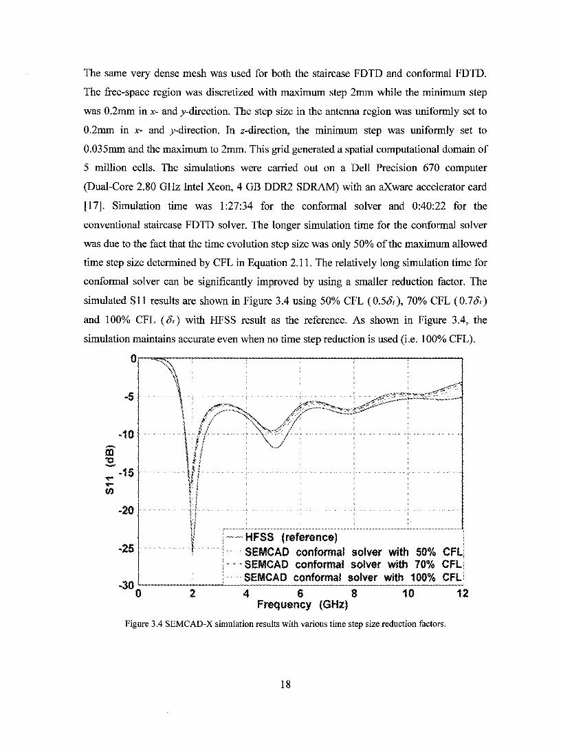
3.4 SEM CAD-X simulation results with various time step size reduction factors ........ 18
3.5 SEMCAD-X simulation results with a coarse grid [29] ............................................ 19
3.6 Geometry and dimension ofthe simulated spiral antenna ..................................... 20
3.7 Simulated S11 (normalized with 1880) using SEMCAD-X staircase FDTD solver and conformaI FDTD solver shown together with the HFSS result as reference ..... 21
4.1 Three-Iayer tissue model: (a) Top view of the three-Iayer tissue model (b) side view of the three-Iayer tissue model (c) 3-D view of the three-Iayer tissue model ...................................................................................................................... 25
4.2 Magnitude of electric field as a function of depth into tissue layer when illuminated by a normal incident plane-wave at (a) 403.5MHz and (b) 6.5GHz with different muscle thickness ........................................................................................................ 26
4.3 CaIculated electric field magnitude using a two-Iayer skin model and a single-layer skin model at (a) 403.5MHz and (b) 6.5GHz ............................................................ 28
vu
4.4 Simulated induced voltage waveform on a voltage sensor using a two-Iayer skin model and a single-layer skin model at (a) 403.5MHz and (b) 6.5GHz ....................................................................................................................... 29
4.5 Geometry and dimension of the modeled wire dipole antenna. Above: wire dipole shown in the x-y plane; Below: wire dipole cross-section view ................................ 30
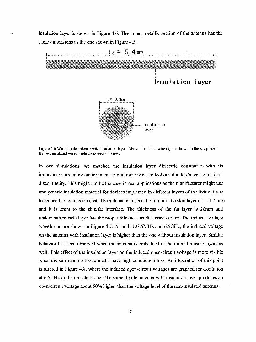
4.6 Wire dipole antenna with insulation layer. Above: insulated wire dipole shown in the x-y plane; Below: insulated dipole cross-section view ....................................... .31
4.7 Simulated induced voltage on the dipole antenna with and without insulation layer at (a) 403.5MHz and (b) 6.5GHz ................................................................................... 32
4.8 Simulated induced voltage on the dipole antenna in muscle layer at 6.5GHz with and without insulation ...................................................................................................... 33
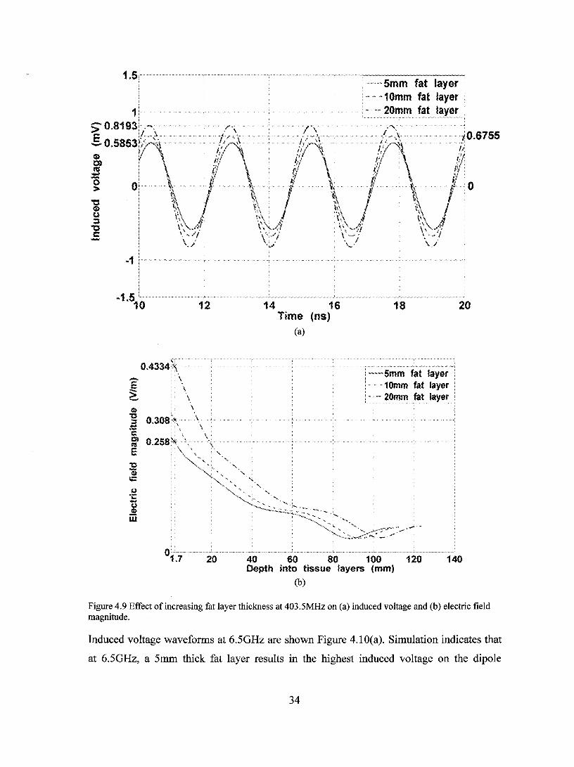
4.9 Effect ofincreasing fat layer thickness at 403.5MHz on (a) induced voltage and (b) electric field magnitude ............................................................................................. 34
4.10 Effect of increasing fat layer thickness at 6.5GHz on (a) induced voltage and (b) electric field magnitude ............................................................................................. 35
4.11 Electric field magnitude distribution at 6.5GHz simulated with SEMCAD-X ........ .36
4.12 (a) Calculated electric field magnitude and (b) simulated induced voltage waveforms at various locations at 403.5MHz ............................................................................. .38
4.13 ( a) Calculated electric field magnitude and (b) simulated induced voltage waveforms at various locations at 6.5GHz ................................................................................... 39
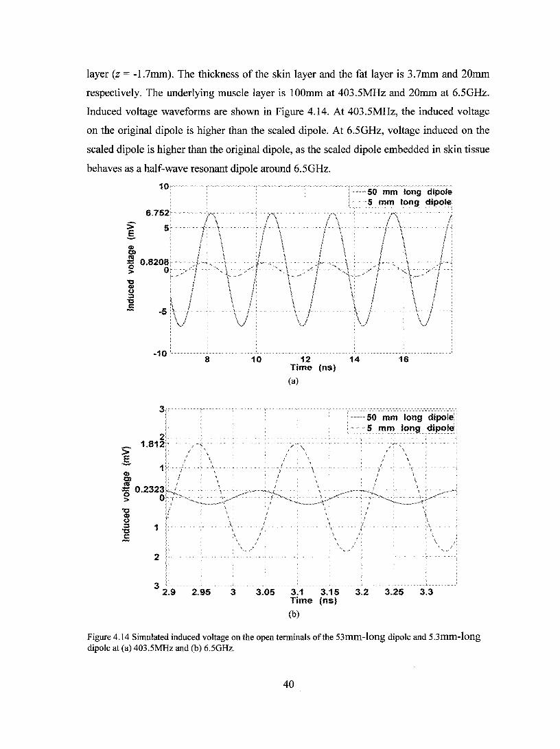
4.14 Simulated induced voltage on the open terminaIs of the 53mm-Iong dipole and 5mm-Iong dipole at (a) 403.5MHz and (b) 6.5GHz ................................................. .40
4.15 Geometry and dimension of the simulated spiral antenna. The antenna is modeled to be 70J.lm thick ............................................................................................................ 41
4.16 Simulated induced voltage waveforms with a LHCP plane-wave and a RHCP plane-wave at (a) 403.5MHz and (b) 6.5GHz .......................................................... .42
4.17 Relative permittivity and conductivity of fat calculated using Cole-Cole model and Debye model. ............................................................................................................. 44
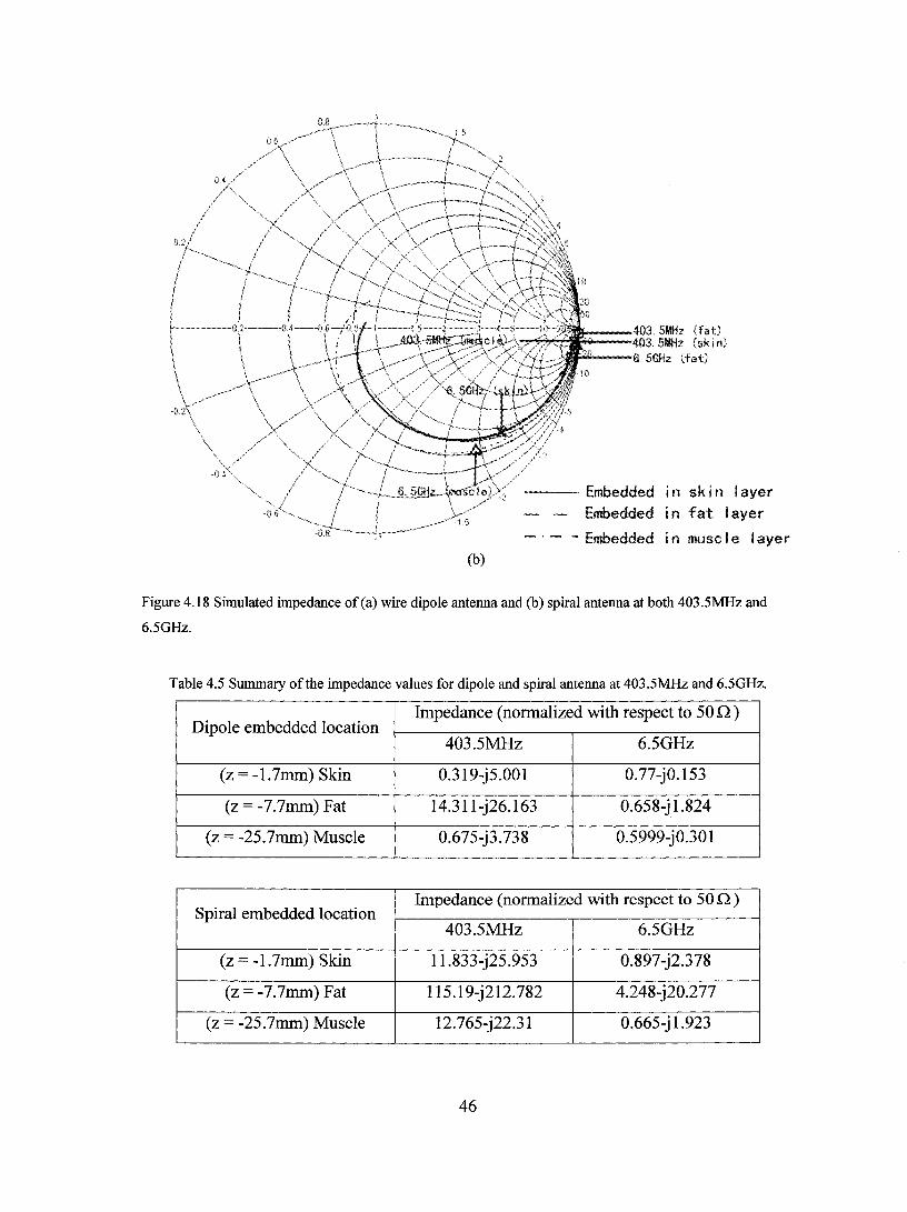
4.18 Simulated impedance of (a) wire dipole antenna and (b) spiral antenna at both 403.5MHz and 6.5GHz .............................................................................................. 46
Vlll
List of Tables
2.1 Summary of sorne existing bio-telemetry systems[5] ................................................ .4
2.2 Parameters of different tissue layers at 403MHz and 6.5GH ................................... 15
3.1 Spatial resolution setup for spiral antenna simulation ............................................... .21
4.1 Exposure limits set up by various agencies for general public (non controlled environment) .............................................................................................................. 22
4.3 Simulated induced peak voltage at various embedded at 403.5MHz and 6.5GHz ....................................................................................................................... 39
4.4 Debye parameters used to mode1 tissue materials .................................................... .44
4.5 Summary of the impedance values for dipole and spiral antenna at both 403.5MHz and 6.5GHz ................................................................................................................ 46
IX
Chapter 1 Introduction Recent research has demonstrated the new areas of antenna applications in biological
devices [1], [2]. In these applications, the antenna is usually in close proximity with
biological structures. In sorne cases, the antenna is implanted in the body [3], [4]. In
particular, our motivation cornes from the emerging technology that aims to use telemetric
systems for neurophysiological research.
Currently there are limits to the technologies to stimulate and acquire data remotely
from a variety of implanted bio-sensors for a relatively long period of time. Alternate
technologies include non-te1emetric solutions where external cab les are used to supply
power to the implanted electrodes and to connect the sensor to the data acquisition system.
Existing telemetric solutions are not designed specifically to provide significant bandwidth
for multi-channe1 high-bandwidth data collection and the wire1ess transmission is usually in
the centimetre range. In the proposed future telemetric solution, the antenna has dual
functionalities including transmitting bio-signaIs to the data acquisition system as weIl as
receiving microwave energy to power any implanted subsystems. One of the main technical
challenges is the design of a miniaturized high-efficiency broadband rectifier-antenna with
re1atively long lifespan. This requires careful studies of the antenna behaviour in the
complex biological tissue structures.
This thesis presents a study of the antenna behaviour in non-homogeneous lossy media
using high-precision electromagnetic simulation software. A brief introduction to the
finite-difference time-domain (FDTD) method (numerical foundation of the SEMCAD-X
tool) is included in Chapter 2 along with the literature review.
In Chapter 3, we present the SEMCAD-X conformaI solver treatment of the curved
boundaries by a cross-platform comparison with HFSS (finite-e1ement-based tool).
Chapter 4 summarizes parametric simulation results to study induced open-circuit
voltage of a simple dipole antenna as weIl as a spiral antenna in layered tissue-like media
with a plane-wave excitation.
Finally in Chapter 5, we make concluding remarks about the work presented here, and
point to possible direction for further investigations.
1
Chapter 2 Background Review
2.1 RF Bio-Telemetry and Antenna Behaviour
A telemetry system is used to colle ct data at a place that is remote or inconvenient to access.
It often utilizes wireless transmitting channels. A typical telemetry system is composed of a
data collection subsystem, a multiplexer, a transmitter/receiver, a de-multiplexer and a data
processing unit [6]. Telemetry itself has a long history of development over 200 years [7].
It has been widely accepted in the field of military applications (e.g. missile tests) and
industrial applications (e.g. power utility monitoring) [7]. However, it is not until the late
1950s that the biologists and physicians started to realize the potential of telemetry for
measuring pH and temperature from internaI cavities [9]. A series of lectures and
demonstrations were organized world-wide by the scientific and engineering communities
from 1960s to 1970s [8], contributing to the overall increase of interest in telemetric system.
In the following sections, a very brief review and introduction to RF bio-sensing telemetry
is presented followed by a section dedicated to a literature survey of antennas embedded in
biological tissues.
2.1.1 RF Bio-Telemetry
Telemetric solution has been used in biological sensing as early as the late 1950s in animal
tests. These early bio-sensing telemetric systems used Hartley oscillator as the basic RF
building block [8]. It has been shown by Mackay and Jacobson in 1957 that a Hartley
oscillator can be configured to work as a pressure sensor as weIl as a temperature sensor in
frequency modulation (FM) [8]. Analog pressure information is modulated onto the carrier
signal as a small variation of the resonant frequency, while temperature information is
represented by a pulse train at a much lower frequency. It is not until 1970s that
measurements from human subjects were shown to be feasible for fetal monitoring in utero,
electrocardiogram (ECG) telemetry and gastrointestinal pressures [9]. In these applications,
bio-sensing telemetry utilizes RF transmitting channels exclusively as it is vital to leave the
2
subject in his normal physiological and psychological state with as little interference as
possible with his normal pattern of activities.
Due to the low data bandwidth required in the early bio-sensing telemetry system, the
transmittinglreceiving antenna is usually a fairly simple resonant structure. Often, it is a
dipole or a loop antenna. In the early systems, antennas were not specifically designed to
work in the biologically embedded environment, but they were rather studied in a
simplified dielectric medium. The design work emphasized the position, orientation and
physical size of the antenna [8] but largely neglected investigations of its interaction with
the living (ho st) tissue. In the early bio-sensing telemetric systems, batteries were used as
the primary power source. This often imposed a trade-off in the design of systems for
long-range animal experiments, as the engineering solution frequently represented a
compromise between transmitter life, size, weight and transmission range [8].
Although the feasibility of using wireless technology to communicate vital signs was
demonstrated more than 30 years ago, the above mentioned limitations in system design
have greatly delayed its wide deployment in both research and clinical applications until
recent advantages in miniaturized, integrated digital system design. In 2000, Gavriel Iddan
et al demonstrated a wireless capsule capable of recording 5,000 images over a period of
7-8 hours and transmit the images back to a wearable antenna array [10]. This system had a
huge impact on scientists and physicians who were puzzled by the small intestine which
was extremely difficult to study using the traditional scope test due to the complicated
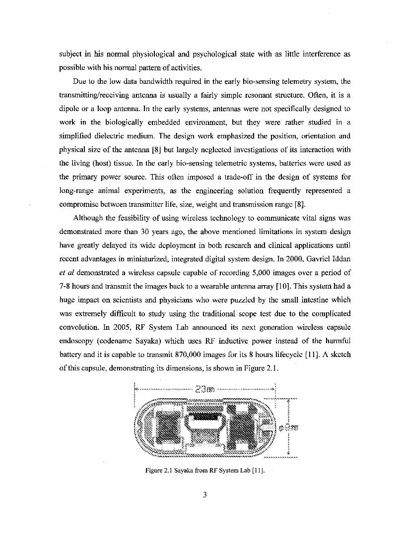
convolution. In 2005, RF System Lab announced its next generation wireless capsule
endoscopy (codename Sayaka) which uses RF inductive power instead of the harmful
battery and it is capable to transmit 870,000 images for its 8 hours lifecycle [11]. A sketch
ofthis capsule, demonstrating its dimensions, is shown in Figure 2.1.
Figure 2.1 Sayaka from RF System Lab [11].
3
Miniaturized bio-sensing telemetry also finds its use in physiological studies. This has
been a particular interest to the National Aeronautics and Space Administration (NASA)
where scientists and engineers are trying to develop telemetric-based implantable sensing
systems to monitor the physiological parameters of astronauts during space flights [5].
These related researches also utilize inductive power as the energy source for the sensor
system. Sorne examples of resulting bio-sensing telemetric systems are summarized in
Table 2.1.
Table 2.1 Summary of sorne existing bio-telemetric systems.
On-Chip Inductor Wireless Link Reference Dimensions (mm) Distance (mm)
2 x 10 30 Von Arx and Najafi [5]
5x5 5 Eggers et al. [5]
10.3 diameter 30 Ullerich et al.
Mokwa and Schnakenberg [5]
1 x 1 100 Rainee et al. [5]
Notice that the existing systems above only have very short transmission ranges in the
order of 1/10th of a meter making them not suitable in sorne cases where relatively long
transmission ranges are required. Due to the relative low operating frequency (VHF band),
a square spiral loop is used as the inductor/antenna combination where the ideas of
transformer are more relevant than the usual considerations of radiation fields [8].
The proposed new system will operate at a higher frequency to pro vide wider data
bandwidth with an extended transmission range in the order of meter. In 1999, Federal
Communications Commission (FCC) and European Telecommunications Standards
Institute (ETSI) standardized Medical Implant Communication Service (MICS) band at
402-405MHz. This frequency band is carefully chosen to avoid interference with other RF
traffic and to minimize the coupling with living tissues. Implanted antennas have also being
designed to operate in the 2.4GHz ISM band. However, due to the high water content in
living tissues, the 2.4GHz band has a relatively high conduction loss; therefore it is not a
favourable choice for implanted antennas. Last proposed frequency band is at 6.5GHz ISM
band [32]. This frequency has the minimum tissue attenuation. In the following section, a
4
brief literature survey of these biologically-embedded antennas is presented after an
introduction to the two common numerical methods used to model these antennas.
2.1.2 Numerical Analysis of Embedded Antenna in Biological Tissue
Antennas used in bio-sensing telemetry function differently from the traditional free-space
operation. Their behaviour must be studied in a manner that includes the complex
biological environment and its interaction with the near-field antenna ration. In the
literature, biological embedded environment is often modeled as a lossy material with high
permittivity. Two numerical methods are commonly used in the analysis. In this section,
we present a brief introduction to both of these two methods followed by sorne published
example antenna analysis results.
2.1.2.1 Spherical Dyadic Green's Functions (DGF)
Spherical DGF is often used to model wire antennas in the human head. In this method, the
human head is represented by a multi-Iayer lossy dielectric sphere as shown in Figure 2.2.
Skin
Fat
Bone
Dura
CSF
Brain
Figure 2.2 Ruman head model [12].
The total electric field E , generated by CUITent density of the implanted source Js, can be
calculated by the volume integration over the source in terms of the spherical dyadic
Green's Functions
(2.1)
where Jis is the permeability of the source layer,
-r(r,B,rp) is the field location,
5
-1
r (ra, (Jo, ((Jo) is the source location,
8fs is the Kronecker delta function,
= --1
GeO(r,r )is an unbounded spherical DGF in the source region, and
=(fs) - -1
Ges (r,r) is a scattering spherical DGF in the field layer from the source.
- -1
The detailed derivation of the formulation together with the expressions of GeO(r, r ) and
=(fs) __ 1
Ges (r,r) can be found in [13], [14], results are also summarized in [12].
To facilitate the numerical implementation of Equation 2.1, the Wlre antenna is
decomposed to represent a superposition of infinitesimal CUITent elements lining up along
the antenna. Each infinitesimal CUITent is then decomposed into a rotated local coordinate
system as shown in Figure 2.3 .
. \
• , \ \
\\~ , , , \
\ , , , \
\ \
+ ,~
t .' " .... ", . "'\ "' .. ..-
\ '\ .i; fi, \ ..... .",
.:.H.
Figure 2.3 Decomposition ofwire antenna with local coordinate rotation [12].
Then, the source integration in Equation 2.1 can be approximated by a finite summation of
the electric field contributions from aU CUITent elements. Each one of the CUITent element
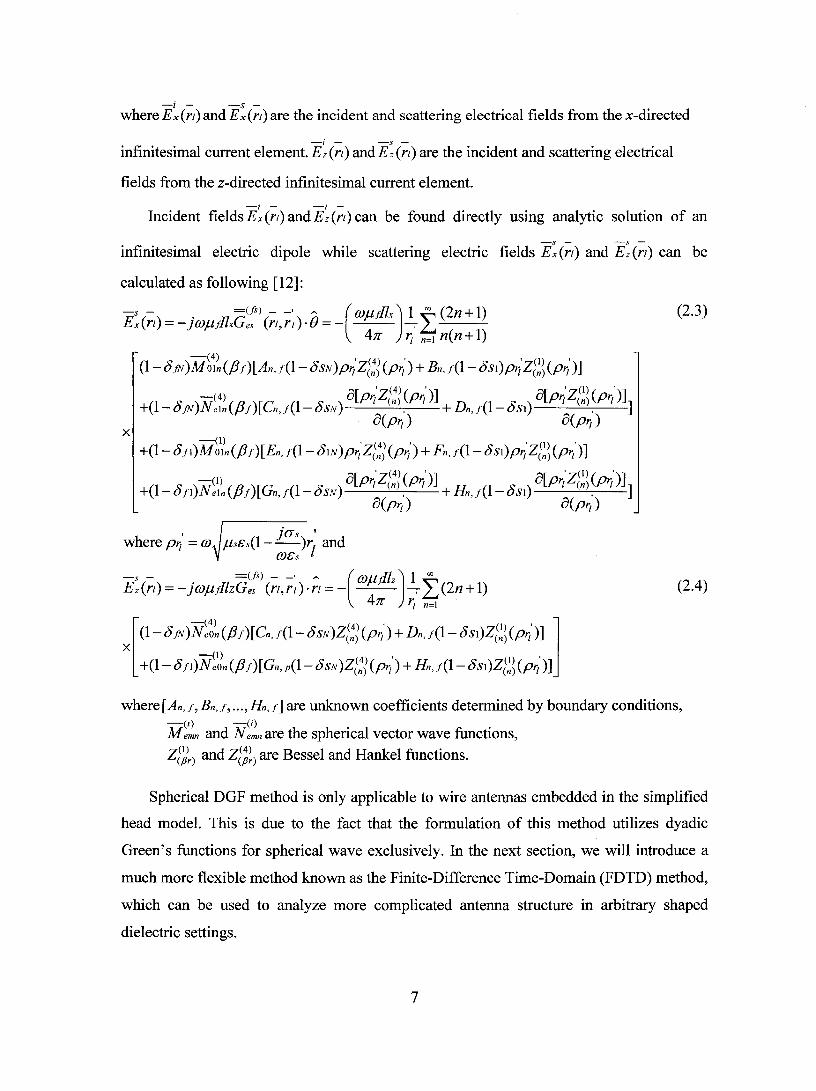
where [An,f, Bn,J, ... , Hn,J] are unknown coefficients determined by boundary conditions, -(il -(il M emn and N emn are the spherical vector wave functions,
Z(~r) and Z~~) are Bessel and Hankel functions.
Spherical DGF method is only applicable to wire antennas embedded in the simplified
head model. This is due to the fact that the formulation of this method utilizes dyadic
Green's functions for spherical wave exclusively. In the next section, we will introduce a
much more flexible method known as the Finite-Difference Time-Domain (FDTD) method,
which can be used to analyze more complicated antenna structure in arbitrary shaped
model is irrelevant. In Chapter 4 of this thesis, we will verify this by comparing the
single-layer skin model with a two-Iayer skin mode!.
The thickness of different tissue layers varies considerably from individual to
individual and from time to time. In literature, skin thickness is normally reported to be in
the range from Imm - 5mm with a typical value close to 3.7mm [2], [12], [18], [22], [23]
while the fat layer is usually treated as a parametric variable from Omm - 15mm [18], [22].
2.2.2 Relative Permittivity and Conductivity of Tissue Layers
Dielectric spectrum of tissues has been weIl studied and summarized in several
publications [20], [24]. In general, permittivity & is a complex function of frequency
written as:
Sc = s' - js" complex pennittivity
• Œ'e =Se-J
O)
13
(2.12)
Ge is the effective permittivity and (J"e is the effective conductivity
Relative permittivity Ger is defined as:
Ce Cer=-
Co
Co =8.8541878176 X 10¹² F/m
Loss due to finite conductivity is expressed as loss tangent
tan8=- Im[cc] =_ ae =_ c" Re[ cc] OJCe c'
(2.13)
(2.14)
Complex permittivity GC can be approximately expressed as a function of frequency by
Debye relaxation expression: Cs - [ft,
Cc = [ft, + j---1+ jarr
where
coo is the permittivity at the high frequency limit,
Cs is the low frequency (static) permittivity,
r is the characteristic relaxation time of the medium.
Hurt modeled the dielectric spectrum of the muscle using a summation of five Debye
dispersions in addition to a conductivity term as followed [25]:
5 Î'1Cn ai Cc = [ft, + l +--
n=1 1 + jOJrn jOJco
where
rn is the n th characteristic relaxation time ofthe medium
Î'16n is the change in the relative permittivity (6s - 600) associated with rn
O'i is the static ionic conductivity
Î'161,Î'162 .. can be normalized respect to one constantÎ'16 and Equation 2.16 becomes
~ An 0-, 6e = 600 + (6s-[ft,)..L.. +--
n=1 1 + jOJrn jOJ60
(2.15)
(2.16)
(2.17)
Due to the complex nature ofbiological tissues, each of the Debye terms is broadened by
introducing an empirical distribution parameter an, the result is known as the multi-term
Cole-Cole expression:
14
~ !J.&n (Yi &c=&oo+ L. +--
n=J (1 + jOJrn)(I-an) jOJ&O (2.18)
where
an is the measure ofhroadening of the dispersion
AlI the constants for the Cole-Cole model can he found in [20]; therefore using Equation
2.18, complex permittivity can he calculated at any given frequency. The folIowing values
are taken from [26] calculated using Equation 2.18 at 403MHz and 6.5GHz with the
exception of the unified skin tissue where the relative permittivity and conductivity are
calculated using the weighted average of the dry skin and wet skin over their thickness.
Table 2.2 Parameters of different tissue layers at 403MHz and 6.5GH.
403MHz 6.5 GHz
Tissue Ber (J" (%) Ber (J" (%)
Muscle 57.104 0.79708 47.544 5.8201
Fat 5.5785 0.041167 4.8917 0.33955
Skin (dry) 46.718 0.68934 34.519 4.3433
Skin (wet) 49.85 0.67004 37.761 5.0544
Skin (averaged) 48.0603 0.6811 35.91 4.6481
15
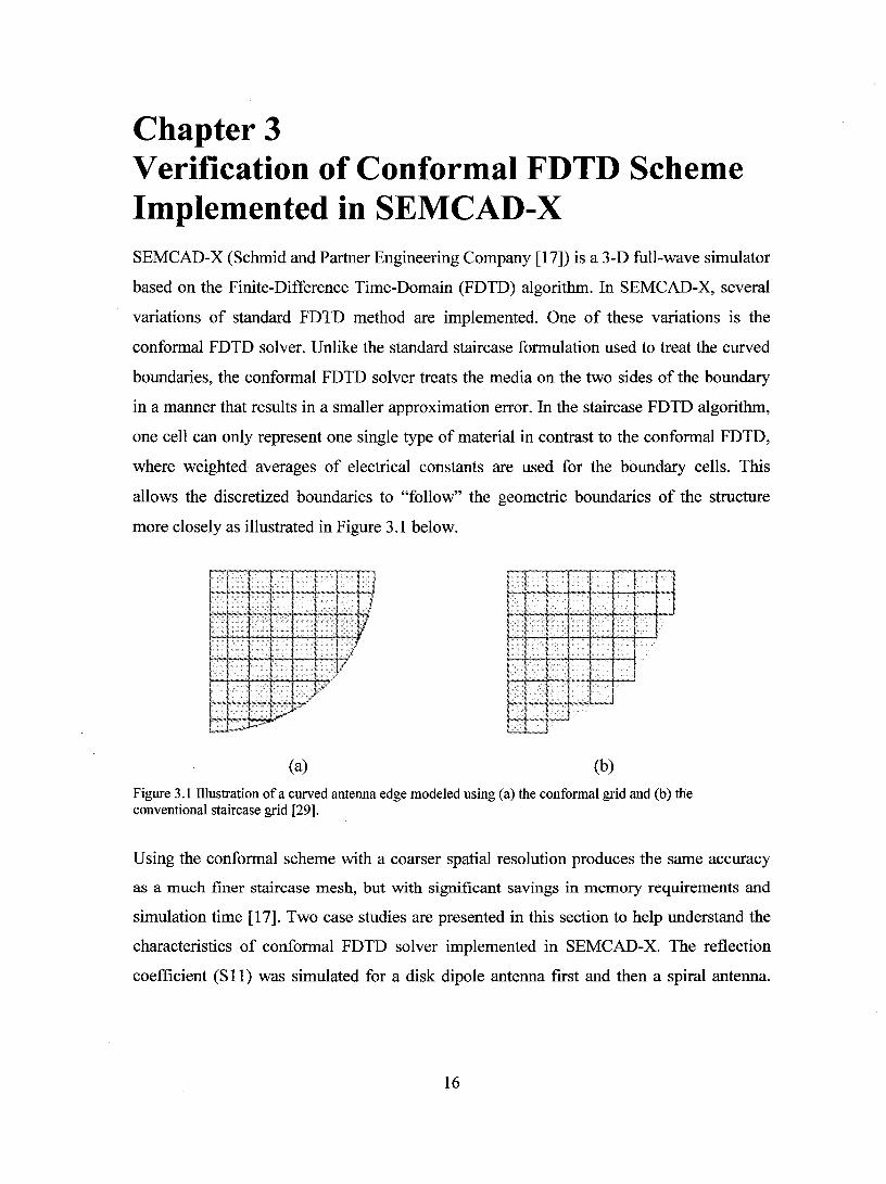
Chapter 3 Verification of Conformai FDTD Scheme Implemented in SEMCAD-X SEMCAD-X (Schmid and Partner Engineering Company [17]) is a 3-D fuIl-wave simulator
based on the Finite-Difference Time-Domain (FDTD) algorithm. In SEMCAD-X, several
variations of standard FDTD method are implemented. One of these variations is the
conformai FDTD solver. Unlike the standard staircase formulation used to treat the curved
boundaries, the conformaI FDTD solver treats the media on the two sides of the boundary
in a manner that results in a smaIler approximation error. In the staircase FDTD algorithm,
one ceIl can only represent one single type of material in contrast to the conformaI FDTD,
where weighted averages of electrical constants are used for the boundary ceIls. This
allows the discretized boundaries to "foIlow" the geometric boundaries of the structure
more closely as illustrated in Figure 3.1 below.
(a) (b)
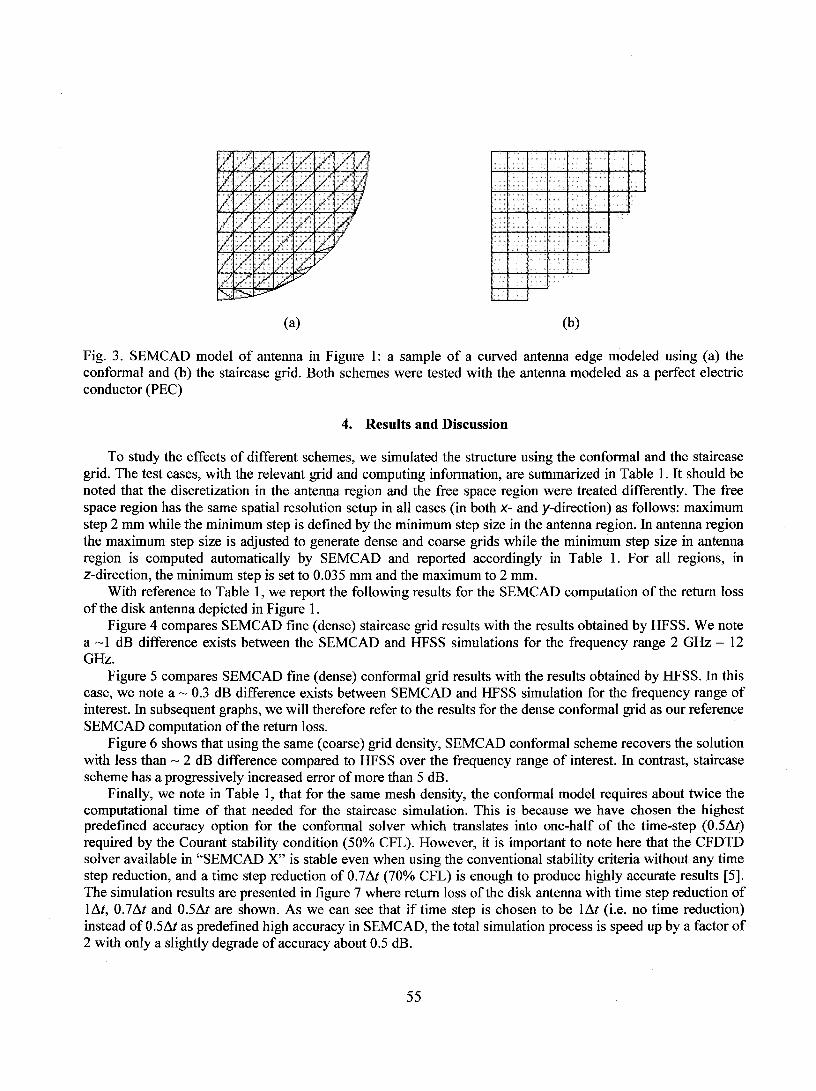
Figure 3.1 Illustration ofa curved antenna edge modeled using (a) the conformaI grid and (b) the conventional staircase grid [29].
Using the conformaI scheme with a coarser spatial resolution produces the same accuracy
as a much tiner staircase mesh, but with signiticant savings in memory requirements and
simulation time [17]. Two case studies are presented in this section to help understand the
characteristics of conformaI FDTD solver implemented in SEMCAD-X. The reflection
coefficient (S Il) was simulated for a disk dipole antenna first and then a spiral antenna.
16
These two antennas were chosen for their curved boundaries which best differentiate the
conformaI and the conventional staircase FDTD soivers.
3.1 Disk Dipole Antenna
The geometry of disk dipole antenna is shown in Figure 3.2 together with its dimension and
its orientation relative to the coordinate system. The antenna is 70llm in thickness with
1mm spacing between disks to accommodate the feed structure. The reflection coefficient
(SIl) was first simulated in HFSS as the reference and then in SEMCAD-X using both
conventionai staircase FDTD soiver and conformaI FDTD sol ver. The simulated S Il in this
section is normalized with respect to 50 Q . The results are shown in Figure 3.3.
30 mm
1 mm
z
X l
/L_~y
Figure 3.2 Geometry, dimension and orientation ofthe simulated disk dipole antenna [29].
Figure 3.7 Simulated SIl (normalized to 188 n) using SEMCAD-X staircase FDTD solver and conformaI FDTD solver shown together with the HFSS result as reference.
21
Chapter 4 Parametric Studies- Results and Discussion Instead of focusing on the radiating characteristics of an antenna, in this section, we focus
on its receiving properties. In particular, this antenna will be used as part of the
rectifier-antenna (i.e. rectenna). As the name suggests, this structure rectifies the received
RF signal to provide its DC component. Therefore, utilizing a rectenna can effectively
eliminate external cables or batteries for the embedded bio-telemetric devices and provide
internaI power source. Preliminary studies of miniaturized rectenna in free-space have been
published [27], [30] and [31]. In this thesis, we demonstrate a study of the receiving
characteristics of the rectenna in the context of its proximity to the biological tissues. Our
test cases are the wire dipole antenna chosen for its structural simplicity and robustness,
and the spiral antenna chosen for its wide bandwidth. The incident wave is a plane-wave
with specified frequency and magnitude. The excitation frequencies of interest are
403.5MHz and 6.5GHz. The magnitude of electric field is set to 1 V/m for aIl cases. This
value is weIl below electromagnetic field exposure limits set by IEEE, FCC and
International Commission on Non-Ionizing Radiation Protection (lCNIRP) outlined in
Table 3.1 at both frequencies.
Table 4.1 Exposure limits set up by various agencies for general public (non controlled environment).
-Power density Equivlent plane wave E
(mW/cm2) field amplitude CV lm)
403.5MHz 6.5GHz 403.5MHz 6.5GHz
IEEE Std C95.1 [33] 0.269 4.33 31.8 127.8
FCC OET Bulletin 65 [34] 0.269 1.0 31.8 61.4
ICNIRP Std, [35] 0.202 1.0 27.6 61.4
4.1 Methodology
There are several variables of particular interest in terms of their effects on the induced
voltage on the receiving antenna terminaIs. These variables are summarized in Table 4.2.
One of the most important parameters is the location where the antenna is embedded. The
22
antennas are simulated when placed in different tissue layers: skin, fat and muscle. Within
the relatively thick fat layer, we examine the antenna at four different locations relative to
its position to the skin/fat interface. For an additional parametric study, we fix the antenna
in the skin layer and vary the thickness of the undemeath fat layer from 5mm to 20mm to
investigate the change of the dielectric distribution in the near-field of the antenna on its
properties. Similar procedure has been reported in [18] and [19]. Both the wire dipole and
the spiral antenna are simulated for the settings noted above. Our further investigations
consider miniaturized dipole and spiral antenna, more appropriate for implant applications.
The dipole antenna is scaled down by 1/1 Oth and the spiral antenna by ~ of their initially
studied size. In practice, metals are not directly implanted in tissues and thus the study of
the insulation layer around the antenna is of particular importance. Literature indicates that
the insulation layer can help improve the radiation efficiency when the antenna is
embedded in a lossy material [18]. Hence, part of our study focuses on detecting any
possible effect of the insulation layer on the induced voltage of the embedded antennas via
simulations. Finally, all the simulations are performed at both 403.5MHz and 6.5GHz. We
selectively present the representing results from our simulations in section 4.3 and 4.4.
Table 4.2 Simulation setup variables.
Variable Value
Type of antenna dipole spiral
Locations of the one location in skin layer (z = -1.7mm)
four locations in fat layer (z = -5.7, -7.7,-11.7, -19.7mm) antenna
one location in muscle layer (z = - 25.7mm)
Thickness of fat layer 5mm,10mm,20mm
Insulation layer with insulation layer without insulation layer
Size of the antenna Original: 53mm (length) Original: 45mm (diameter)
Scaled:5.3mm (length) Scaled: 22.7mm (diameter)
Excitation frequency 403.5MHz 6.5GHz
23
4.2 Simulation Model Verifications
Three-layer tissue model is shown in Figure 4.1. The exciting plane-wave signal is
propogating in -z direction (i.e. perpendicular into the plane of the page) within the
plane-wave excitation region.
y
Plane-wave excitation region
(a) Top view of the three-layer tissue model
(b) Side view of the three-layer tissue model
24
(c) 3-D view of the three-layer tissue model
Figure 4.1 Three-layer tissue mode!.
4.2.1 Thickness of Muscle Layer
Ideally, Absobing Boundary Conditions (ABCs) should be applied on the four side-walls as
well as the bottom face of the model to elminate reflecting waves. However, due to the
limitation of the aXware accerelator card on the computers available, this model cannot be
implement when plane-wave excitation is used. For the side-walls, as the incident wave is
propagating in the -z direction, we assume that the reflection from these faces is small
enough to be safely neglected as they are mainly reflection of scattering field caused by the
embedded antenna structure. To eliminate the reflection from the bottom muscle/air
interface, we use a muscle layer with extended thickness such that the conduction loss
introduced by the finite conductivity of the muscle consumes most of the wave energy,
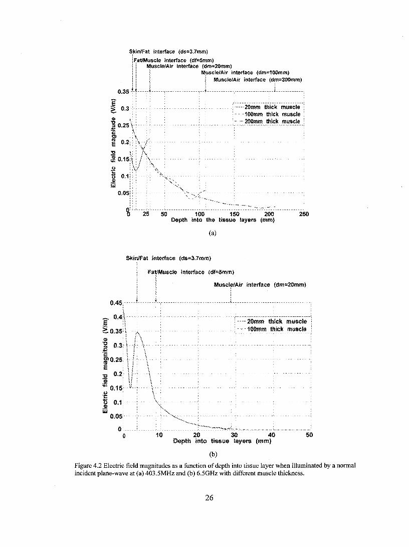
reducing the reflected wave to a negligible level. To valide the thickness of muscle layer
required to safely ignore the reflection from the bottom, a Matlab script is wrtten to
calculate the I-D electric field magnitude as a function of z (depth into the tissues) (see
Appendix B). The program utilizes the continuity of tangential electric field and magnetic
field on dielectric boundaries to form a set of linear equations. Solving these equations
gives the magnitudes of the electric field at these boundaries. The complete solution can
then be interpolated according to the theoretical formula. The magnitude of electric field
across tissue layers are shown in Figure 4.2.
25
~kin/Fat interface (ds=3.7mm)
IFatlMuscle interface (df=5mm)
Il Muscle/Air interface (dm=20mm) , Muscle/Air interface (dm=100mm)
11 l 1 Muscle/Air interface (dm=200mm) l ' 1
0.35 t 1 t
0.45;
ri 25 50
""-- 20mm thick muscle .. " -100mm thick muscle
'- -- 200mm thick muscle
-,-,- -~ ~- -- ... -' -,..."
100 150 200 250 Oepth into the tissue layers (mm)
(a)
SkïnlFat interface (ds"'3.7mm) i
Fat/Muscle
1
J
interface (df=5mm)
MU$cl~/Air interface (dm=20mm)
~"- 20mm thick muscle ." -100mm thick
0·············_· .. ·········· o 10 20 30 40 50
Oepth into tissue layers (mm)
(b)
Figure 4.2 Electric field magnitudes as a function of depth into tissue layer when illuminated by a normal incident plane-wave at (a) 403.5MHz and (b) 6.5GHz with different muscle thickness.
26
As shown in Figure 4.2(a), at 403.5MHz the magnitude of electric filed changes
significantly when the thickness of muscle layer varies from 20mm to lOOmm. However,
the magnitude of eleetrie field does not change very mueh when the thiekness of the muscle
layer grows from lOOmm to 200mm. This statement is especially true when the magnitude
of electric field is measured at depth into the tissues smaller than 25mm. From these results
we infer that a lOOmm thick muscle layer (dm = lOOmm) is sufficient to eliminate
unwanted reflections from the muscle/air interface through the loss meehanism at
403.5MHz. At 6.5GHz, we expect that, due to higher conductivity loss (Table 2.2), a
thinner muscle layer should provide sufficient attenuation to safely ignore the reflection
from the bottom muscle/air interface. This is clearly confirmed by the overlap of relevant
results graphed in Figure 4.2(b). As a conclusion for 6.5GHz, a 20mm thick muscle layer
( dm = 20mm) is sufficient to reduce the reflection from the bottom muscle/air interface to
a negligible level and thus emulate the absorbing boundary conditions.
4.2.2 The Effect of Spatial Resolution on the Skin Layer
The skin layer shown in Figure 4.1 (b) ean be further deeomposed into wet skin and dry
skin. They have slightly different relative permittivities as shown in Table 2.2. The
thickness ofwet skin is around 1.5mm and that of the dry skin is approximately 2mm [36].
However, we expect that this marginal increment of spatial resolution on the skin layer
should not have a signigicant effeet on our simulations. This statement holds true at both
403.5MHz and 6.5GHz, as the wavelengths corresponding to both frequencies in the
dielectric environment are much larger than the thickness of the skin layer. Therefore, the
wave can hardly distrigush between wet skin and dry skin. To validate the single-layer skin
model, a two-Iayer skin model is tested for a comparision. The thickness of single-layer
skin is 3.7mm (ds = 3.7mm) with undemeath fat layer of 20mm (d! = 20mm), and the
muscle layer has the thickness described in previous section. The magnitude of electric
field is again calculated using the Matlab script described in previous section. Results are
shown in Figure 4.3. Field calculations confirm that the single-layer skin model with
averaged (&er,(J) is accurate enough to model the field distributions at 403.5MHz and
5 1 0 15 20 25 30 Depth into the tissue layers (mm)
(b)
Figure 4.3 Calculated electric field magnitude using a two-Iayer skin model and a single-layer skin model at (a) 403.5MHz and (b)6.5GHz.
Further simulations in SEMCAD-X confirm that an ideal voltage sensor embedded in
the single-layer skin mode! and the two-layer skin mode! yeilds practically identical
28
induced voltage level as shown in Figure 4.4. The voltage sensor is embedded 1.7mm into
the skin layer (z = -1.7mm). This again confirms that the detailed, two-Iayer skin mode!
may not be necessary to use for accurate results.
>' E -
-0.2
. ..... single.layer skin model ···_······two-Iayer skin model
10 15 Time (ns)
(a)
..... single-layer single model
' ................. _ ....................... !.. •.••••••••.•••.•••••••••.••••••••••••• i ................................ ~ two-:!l:Iy~~~kin model 1.5 1.6 1.7 1.8 1.9 2
Time (ns)
(b)
Figure 4.4 Simulated induced voltage waveform on a voltage sensor using a two-Iayer skin model and a single-layer skin model at (a) 403.5MHz and (b) 6.5GHz.
29
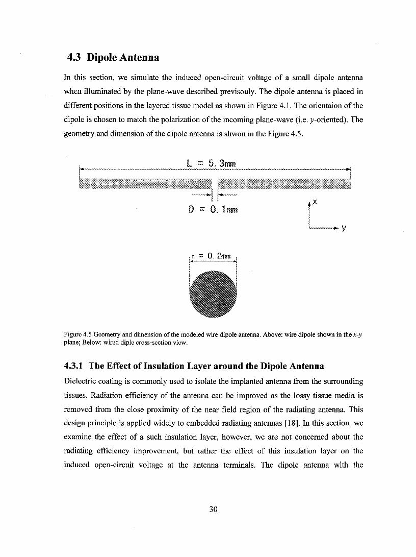
4.3 Dipole Antenna
In this section, we simulate the induced open-circuit voltage of a small dipole antenna
when illuminated by the plane-wave described previsouly. The dipole antenna is placed in
different positions in the layered tissue model as shown in Figure 4.1. The orientaion of the
dipole is chosen to match the polarization of the incoming plane-wave (i.e. y-oriented). The
geometry and dimension of the dipole antenna is shwon in the Figure 4.5.
L 5,3tnm
o ::::: 0, lmm
r :: O.2mm
Figure 4.5 Geometry and dimension ofthe modeled wire dipole antenna. Above: wire dipole shown in the x-y plane; Below: wired diple cross-section view.
4.3.1 The Effect of Insulation Layer around the Dipole Antenna
Dielectric coating is commonly used to isolate the implanted antenna from the surrounding
tissues. Radiation efficiency of the antenna can be improved as the lossy tissue media is
removed from the close proximity of the near field region of the radiating antenna. This
design principle is applied widely to embedded radiating antennas [18]. In this section, we
examine the effect of a such insulation layer, however, we are not concemed about the
radiating efficiency improvement, but rather the effect of this insulation layer on the
induced open-circuit voltage at the antenna terminais. The dipole antenna with the
30
insulation layer is shown in Figure 4.6. The inner, metallic section of the antenna has the
same dimensions as the one shown in Figure 4.5.
L2 = 5.4mm
rz::: O.3mm
Insulation layer
Insulation layer
Figure 4.6 Wire dipole antenna with insulation layer. Above: insulated wire dipole shown in the x-y plane; Below: insulated wired diple cross-section view.
In our simulations, we matched the insulation layer dielectric constant Ber with its
immediate surrending environment to minimize wave reflections due to dielectric matieral
discontinuity. This might not be the case in real applications as the manifacturer might use
one generic insulation material for devices implanted in different layers of the living tissue
to reduce the production cost. The antenna is placed 1.7mm into the skin layer (z = -1.7mm)
and it is 2mm to the skin/fat interface. The thickness of the fat layer is 20mm and
undemeath muscle layer has the proper thickness as discussed earlier. The induced voltage
waveforms are shown in Figure 4.7. At both 403.5MHz and 6.5GHz, the induced voltage
on the antenna with insulation layer is higher than the one without insulation layer. Smiliar
behavior has been observed when the antenna is embedded in the fat and muscle layers as
well. This effect of the insulation layer on the induced open-circuit voltage is more visible
when the surrounding tissue media have high conduction loss. An illustration of this point
is offered in Figure 4.8, where the induced open-circuit voltages are graphed for excitation
at 6.5GHz in the muscle tissue. The same dipole antenna with insulation layer produces an
open-circuit voltage about 50% higher than the voltage level of the non-insulated antenna.
-1.51'0 ......... ...... m· ........................... m ...... , ....................................................... m' .............. mm ... m ..................................................... m ••••••••
Figure 4.16 Simulated induced voltage waveforms with a LHCP plane-wave and a RHCP plane-wave for two frequencies ofinterest: (a) 403.5MHz and (b) 6.5GHz.
42
At 403.5MHz, the spiral antenna is linearly polarized, therefore, the wave reception
resulted in approximately the same level of voltage from either RHCP incoming
plane-wave or LHCP incoming plane-wave. However, at 6.5GHz, the spiral antenna itself
is circularly polarized, therefore, the induced voltages are signiciantly different between the
RHCP incoming wave and LHCP incoming wave. Figure 4.16(b) suggests that this spiral
antenna is LHCP at this frequency.
4.5 Impedance Consideration - Dipole and Spiral Antenna
For maximum power transfer, the impedance of the antenna must match with the
impedance of the rectifier in the next stage in a complex conjugate manner. In this section,
we excite the antenna structure with an edge source and simulate the feed point impedance.
Due to the broadband nature of this group of simulations, the dispersive characteristics of
the tissue materials must be taken into account. In section 4.5.1, we discuss how the
dispersive material can be implemented in SEMCAD-X and in section 4.5.2 we show the
simulated impedance results.
4.5.1 Cole-Cole to Debye model Conversion for Dispersive material
Due to the time-domain nature, FDTD scheme cannot handle the multi-term Cole-Cole
expression (Equation 2.18) with ease. This difficulty originates largely from the fact that
the empirical distribution parameter an is introduced as a fraction number in the exponent.
This fractional exponent translates itself into time domain as the sol ver needs to access
field data at unavailable time instance that is in-between the integer time steps of the FDTD
scheme. Therefore, SEMCAD-X does not support Cole-Cole model directly for the
dispersive material. Unfortunately, most of the parameters found to model dispersive tissue
media are for the Cole-Cole model [20]. Therefore, a mathematical conversion from the
Cole-Cole model ta the Debye model (Equation 2.17) is necessary if a broadband
simulation involving dispersive material is needed. An algorithm developed in [37]
accomplishes this conversion by using Minimum Square Error (MSE) curve fitting
technique. MSE is applied to fit a Debye model to the data points calculated using the
Cole-Cole model. A Matlab implementation of this algorithm is developed and presented in
43
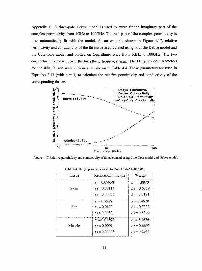
Appendix C. A three-pole Debye model is used to curve fit the imaginary part of the
complex permittivity from 1 GHz to 100GHz. The real part of the complex permittivity is
then automatically fit with the model. As an example shown in Figure 4.17, relative
permittivity and conductivity of the fat tissue is calculated using both the Debye model and
the Cole-Cole model and plotted on logarithmic scale from 1 GHz to 100GHz. The two
curves match very well over the broadband frequency range. The Debye model parameters
for the skin, fat and muscle tissues are shown in Table 4.4. These parameters are used in
Equation 2.17 (with n = 3) to calculate the relative permittivity and conductivity of the
corresponding tissues.
10 Frequency (GHz)
100
Figure 4.17 Relative permittivity and conductivity of fat calculated using Cole-Cole model and Debye model.
Table 4.4. Debye parameters used to model tissue materials.
Tissue Relaxation time (ns) Weight
Tl =0.07958 AI =1.8870
Skin T2 = 0.00114 A2 = 0.6759
T3 = 0.00035 A3 = 0.3121
Tl =0.7958 Al = 1.4628
Fat T2 = 0.0133 A2 = 0.5332
T3 =0.0032 A3 = 0.3599
Tl = 0.01592 AI =3.1676
Muscle T2 = 0.0001 A2 = 0.6695
T3 = 0.00003 A3 =0.2965
44
4.5.2 Impedance of Dipole and Spiral Antenna
In this section, we present the simulated impedances for the dipole antenna and the spiral
antenna when they are embedded in different tissue layers. The two antennas have the same
dimension and geometry as shown in Figure 4.5 and Figure 4.15 respectively. The
impedances are shown on the Smith chart with normalization to 50 n. The markers
indicate the impedances at both 403.5MHz and 6.5GHz. The results are shown in Figure
4.18 and numerical summaries are shown in Table 4.5.
As the Smith chart suggests, the 5mm-Iong dipole in muscle or skin layer is relatively
easy to match at 6.5GHz as it behaves as a resonant half-wave dipole around this frequency.
Spiral antenna is much more difficult to match, especially at 403.5MHz. We also notice
that, without insulation layer, the spiral no longer operates as a frequency independent
antenna in the lossy dielectric media.
(a)
45
""--403, 5111Hz (sk in)
(muscle)
--- Embedded in sk j n 1 ayer Embedded in fat layer
--- Embedded j n sk i n 1 ayer Embedded in fat layer
- ,- - Embedded i n musc 1 e 1 ayer
Figure 4.18 Simulated impedance of (a) wire dipole antenna and (b) spiral antenna at both 403.5MHz and
6.5GHz.
Table 4.5 Summary of the impedance values for dipole and spiral antenna at 403.5MHz and 6.5GHz.
Dipole embedded location Impedance (normalized with respect to 50 n)
403.5MHz 6.5GHz
(z = -1.7mm) Skin 0.319-j5.001 0.77-jO.153
(z = -7.7mm) Fat 14.311-j26.163 0.658-j 1.824
(z = -25.7mm) Muscle 0.675-j3.738 0.5999-jO.301
Spiral embedded location Impedance (normalized with respect to 50 n)
403.5MHz 6.5 GHz
(z = -1.7mm) Skin 11.833-j25.953 0.897-j2.378
(z = -7.7mm) Fat 115.l9-j212.782 4.248-j20.277
(z = -25.7mm) Muscle 12.765-j22.31 0.665-j 1.923
46
Chapter 5 Conclusions and Directions for Future Work In this work, we studied the possibility of utilizing an antenna as part of the
rectifier-antenna system to power up implants for bio-te1emetry applications. To design
such system, it is important to study the behaviour of antennas when embedded in
biological tissues. In particular to this thesis, we studied the induced open-circuit voltage
when the antenna was embedded in different locations in a layered-tissue model and
illuminated by a plane-wave.
We first built the c1assic three-layer tissue model in SEMCAD-X, electromagnetic
simulation tool based on the finite-difference time-domain method. To complete this
layered tissue mode1, we then verified the necessary muscle layer thickness which would
be sufficient to yie1d negligible reflections from the muscle/air interface (mode1 boundary)
through the propagation loss mechanism. FinaIly, we determined that at our chosen
frequencies, it was unnecessary to resolve the skin tissue beyond its single-layer mode1
with dielectric constants that combines, in an average-sense, the dielectric constants of
individual thinner layers.
Next, a simple wire dipole antenna and a spiral antenna were embedded and
illuminated with a plane-wave. Each of the two antennas had two versions with different
physical sizes. AIl four antennas were simulated with and without an insulation layer at
both 403.5MHz and 6.5GHz. In total, we simulated 16 groups of antennas and for each
group, the antenna was placed at various locations in the tissue mode!. A linearly polarized
1 V /m plane-wave was used to illuminate the structure and the induced terminal voltage was
observed for aIl cases. From the observed results, we conc1ude the following:
• At 403.5MHz, the magnitude of electric field is a decreasing function as the
depth into tissues increases. Therefore, as expected, the induced voltage drops
when the antenna is placed deeper and deeper into the tissue layers. Another
observation at this frequency indicates that within our fat layer thickness range
[5mm-20mm], induced open-circuit voltage on a skin-layer-embedded antenna
terminais increases when the thickness of undemeath fat layer increases;
47
• At 6.5GHz, the electric field distribution is very sensitive to the location
(depth) where the observation is made. From a practical point of view, this high
sensitivity might be problematic because very little variation in the location could
cause significant change of the induced voltage on the antenna terminaIs;
• For the wire dipole antenna, the highest induced voltage resulted from the
original size dipole (53mm-Iong) at 403.5MHz. However, if limited by physical
size to the short dipole (5.3mm-dipole), the maximum induced voltage happens at
6.5GHz. For spiral antenna, the general conclusion foIlows the same pattern as the
dipole antenna;
• For aIl the cases, using an insulation layer has a desirable effect on the
induced open-circuit voltage at both frequencies, in the sense of increased induced
terminal voltage with respect to the case of no insulation. As expected, this effect
is more notable when the antenna is placed in a very lossy material.
The work presented in this thesis has demonstrated the potential and limitations of
using an antenna to receive RF energy when embedded in biological (tissue) complex
media. From the simulations, we can estimate that power received by one single antenna is
not sufficient to power up existing implanted devices. Further, we suggest the following
directions for future studies:
• Design of novel miniaturized broadband antenna structure that can be easily
matched at 403.5MHz in a biologicaIly embedded environment;
• Identification of difficulties and related strategies when the incident wave is
randomly polarized and/or from a randomly-incident angle;
• Design an antenna array instead of a single antenna element to coIlect the
impinging wave. This strategy is clearlylinked to the first suggestion, as the size
of the antenna element within the array needs to be further decreased.
Utilizing a miniaturized implanted antenna to receive RF energy to power up a
bio-telemetry system is a novel technique still at its infant stage. We hope that our work
will contribute to the future development of systems that can effectively replace the usage
of batteries and cables in the bio-telemetry systems, allowing for advanced research in
neurophysiology and the consequent applications.
48
References [1] Negar Tavassolian, "Imaging Breast Tumors with Microwaves:
Simulation-Based Assessment of Detection Capabilities of a Broadband Antenna-Sensor", Master Thesis, August 2004.
[2] Jaehoon Kim, Yahya Rahmat-Samii, "Implanted Antennas Inside a Human Body: Simulations, Designs, and Characterizations", IEEE Transactions on Microwave Theory and Technique, vol. 51, pp. 1934-1943, August 2004.
[3] N.H. Ismail, H.D. Ramadan, "Radiation of electromagnetic waves by a circular phased aperture antenna for neck hyperthermia", Radio Science Conference, 2001. NRSC 2001. Proceedings of the Eighteenth National, vol. 2, pp. 653-660, March 2001.
[4] Jaehoon Kim, Yahya Rahmat-Samii, "An Implanted Antenna in the Spherical Human Helad: SAR and Communication Link Performance", IEEE Topical Conference on Wireless Communication Technology, 2003.
[5] R.N. Simons, D.G. Hall, F.A. Miranda, "RF Telemetry System for an Implantable Bio-MEMS Sensor", Microwave Symposium Digest, 2004 IEEE MTT-S International, vol. 3, pp. 1433- 1436, June 2004.
[6] Frank Carden, Telemetry Systems Design, Artech House 1995.
[7] Frank Carden, Russell Jedlicka, Robert Henry, Telemetry Systems Engineering, Artech House 2002.
[8] Mackay R.S., Bio-Medical Telemetry: Sensing and Transmitting Biological Information !rom AnimaIs and Man, IEEE Press 1993.
[9] Thomas F. Budinger, "Biomonitoring with wireless communications", Annu Rev Biomed Eng, 5:383-412, 2003.
[10] Iddan G, Meron G, GlukhovskyA, Paul Swain, "Wireless capsule endoscopy", Nature Vo1.405 ppAO-417, May 2000.
[11] RF SYSTEM website at http://www.rfàmerica.comJ
[12] Yahya Rahmat-Samii and Jaehoon Kim, Implanted Antennas in Medical Wireless Communications, Morgan & Claypool Publishers, June 2006.
[13] L. Li, P. Kooi, M. Leong, and T. Yeo, "Electromagnetic dyadic Green's function in spherically multilayered media" IEEE Transactions on Microwave Theory and Technique, vol. 42, no. 12, pp. 2302-2310, Dec. 1994.
49
[14] C. T. Tai, Dyadic Green's Functions in Electromagnetic Theory, Scranton, PA: Intext Education, 1971.
[15] K.S. Lee, "Numerical solution of initial boundary value prob1ems involving Maxwell's equations in isotropie media," IEEE Transactions on Antennas and Propagation, vol. 14, no.3, pp. 302-307, May 1966.
[16] D.M. Sullivan, Electromagnetic Simulation Using the FDTD method, IEEE Press Series on RF and Microwave Technology, 2000.
[20] C Gabriel et al, "The dielectric properties of biological tissues: III. Parametric models for the dielectric spectrum of tissues", Phys Med Biol. VolAI Issue Il, pp.2271-2293. 1996 Nov.
[21] William G. Scanlon, J. Brian Burns, and Noel E. Evans, "Radiowave Propagation from a Tissue Implanted Source at 418 MHz and 916.5 MHz", IEEE Transaction on Biomedical Engineering, vol.47, noA, pp527-534, April 2000.
[22] Ronold King, Sheila Prasad, Barbara Sandler, "Transponder Antennas In and Near a Three-Layered Body", IEEE Transactions on Microwave Theory and Technique, vol.28, no.6, pp.586-596, June 1980.
[24] Foster and Schwan, "Dielectric properties of tissues and. biological materials: a critical review", Crit.Rev. Biomed Eng. 1725-104.
[25] William D. Hurt, "Muliterm Debye Dispersion Relations for Permittivity of Muscle", IEEE Transaction on BioMedical Engineering, vol. 32, no.1, pp60-64, January 1985.
[26] Italian National Research Council, Institute for Applied Physics, Dielectric Properties of Body Tissue project website at http://niremf.ifac.cnr.it/tissprop/htmlclielhtmlc1ie.htm.
[27] Joseph A. Hagerty, B. Helmbrecht, William H. McCalpin, Regan Zane and Zoya B. Popovié, "Recycling Ambient Microwave Energy With Broad-Band Rectenna Arrays", IEEE Transactions on Microwave Theory and Technique, vol.52, no.3, pp. 1014-1024, March 2004.
50
[28] Constantine A. Balanis, Antenna Theory - Analysis and Design, Chapter Il, John Wiley & Sons, Inc.
[29] Houssam Kanj, Yi Zhang and Milica Popovié, "Advantage of Modeling Broadband Antennas with "SENCAD X" FDTD ConformaI Solver", accepted for ACES 2007 Conference, Verona, Italy, April 2007.
[30] Florian B. Helmbrecht, "A Broadband Rectenna Array for RF Energy Recycling", Diplom-Ingenieur (TU-M··unchen) thesis, Septemer 2002.
[31] Joseph A. Hagerty, Branko D. Popovié and Zoya B. Popovié, "Broadband Rectenna Arrays for Randomly Polarized Incident Waves", 30th European Microwave Conference, pp. 13-1 6, 2000.
[32] United States Frequency Allocation: http://www.ntia.doc.gov/osmhome/allochrt.pdf
[33] IEEE Std C95.1, 1999 Edition: IEEE Standard for Safety Levels with Respect to Human Exposure to Radio Frequency Electromagnetic Fields, 3 kHz to 300 GHz, IEEE, New York, NY, 1999.
[34] FCC OET Bulletin 65 Edition 97-01: Evaluating Compliance with FCC Guidelines for Human Exposure to Radiofrequency Electromagnetic Fields, FCC, Washington D.C., 1997.
[35] ICNIRP Guidelines: Guidelines for Limiting Exposure to Time-Varying Electric, Magnetic, and Electromagnetic Fields (up to 300 GHz), Health Physics, vol. 74, no. 4, pp. 494-522, 1998.
[36] Centre ofbiomedical Technology and Physics, Medical University Vienna http://www.meduniwien.ac.atlzbmtp/bmtlhome.htm.
[37] David F. Kelley and Raymond J. Luebbers, "Debye Function Expansions of Empirical Models of Complex Permittivity for Use in FDTD Solutions", IEEE Antennas and Propagation Society International Symposium, 2003. IEEE Publication vol. 4, pp. 372- 375, June 2003
51
AppendixA Related Publications
• H. Kanj, Y. Zhang and M. Popovic, " Advantage of Modeling Broadband
Antennas with "SENCAD X" FDTD ConformaI Solver If, ACES 2007
Conference, Verona, Italy, April 2007
52
Advantage of Modeling Broadband Antennas with "SENCAD X" FDTD Conformai Solver
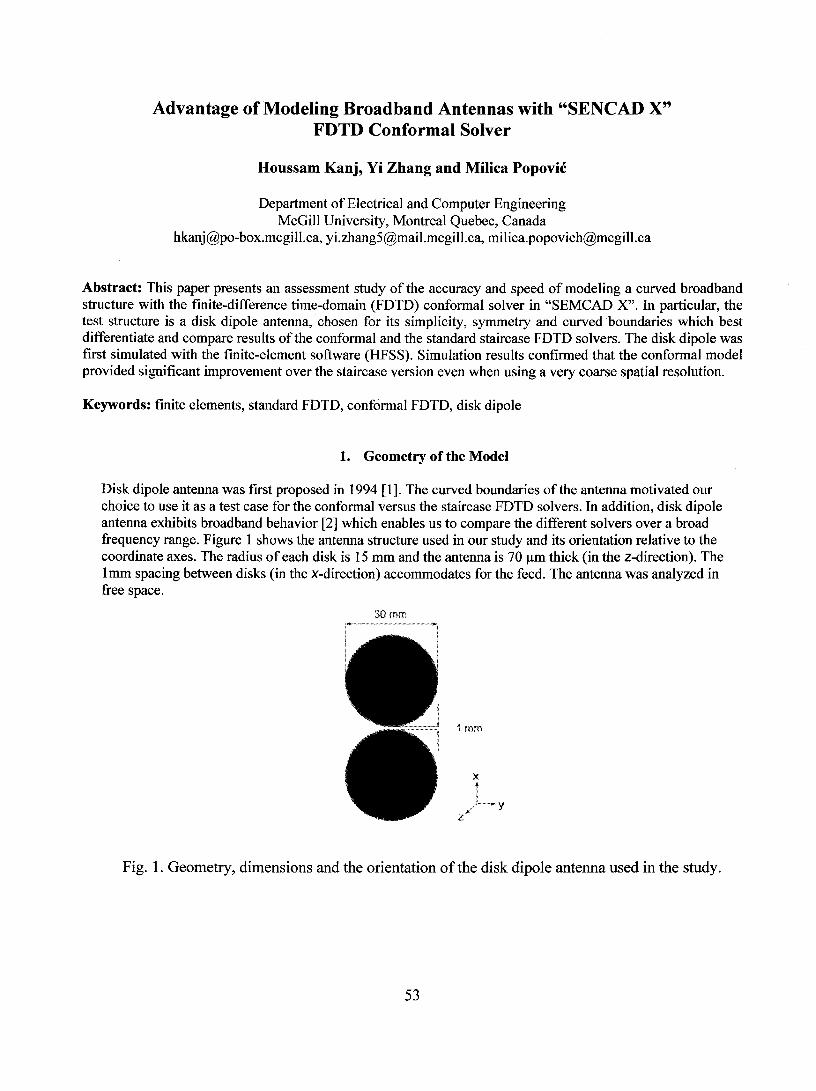
Houssam Kanj, Yi Zhang and Milica Popovié
Department of Electrical and Computer Engineering McGill University, Montreal Quebec, Canada
Abstract: This paper presents an assessment study of the accuracy and speed of modeling a curved broadband structure with the finite-difference time-domain (FDTD) conformai solver in "SEMCAD X". In particular, the test structure is a disk dipole antenna, chosen for its simplicity, symmetry and curved boundaries which best differentiate and compare results of the conformai and the standard staircase FDTD solvers. The disk dipole was first simulated with the finite-element software (HFSS). Simulation results confirmed that the conformai model provided significant improvement over the staircase version even when using a very coarse spatial resolution.
Keywords: finite elements, standard FDTD, conformai FDTD, disk dipole
1. Geometry of the Model
Disk dipole antenna was frrst proposed in 1994 [1]. The curved boundaries of the antenna motivated our choice to use it as a test case for the conformai versus the staircase FDTD solvers. In addition, disk dipole antenna exhibits broadband behavior [2] which enables us to compare the different solvers over a broad frequency range. Figure 1 shows the antenna structure used in our study and its orientation relative to the coordinate axes. The radius of each disk is 15 mm and the antenna is 70 !lm thick (in the z-direction). The Imm spacing between disks (in the x-direction) accommodates for the feed. The antenna was analyzed in free space.
30 mm
1 rmn
Fig. 1. Geometry, dimensions and the orientation ofthe disk dipole antenna used in the study.
53
2. Finite-Element Simulation
The disk dipole antenna described in the previous section was initially simulated in HFSS [3]. HFSS is based on a full-wave finite-element method (FEM), intrinsically conformai in its mesh generation. Two types of metallic materials were used for simulations: copper, with electric conductivity o-Cu= 5.8xl07 Sim and relative permeability J1r-cu = 0.999991 and the perfect electric conductor (PEC). The feed structure was modeled as a lump port on a rectangular section of size 0.07 mm x 1 mm. A radiation boundary was constructed on the surfaces of a large free-space box containing the disk dipole antenna. The structure was analyzed at 12 GHz with a frequency sweep from 0.5 GHz - 12 GHz. Two metallic types yield nearly identical return loss S11 results as graphed in Figure 2. This outcome is expected due to very small conduction loss of copper in the specified frequency range. Next, we simulated the same structure with the FDTD software using the conformai and standard FDTD methods and compared the results with HFSS PEC as the reference.
Fig. 2. Finite-element method results (HFSS): Retum loss of the antenna in Figure 1 modeled as perfect electric conductor (PEC) or as copper, with o-Cu = 5.8xl07 Sim and relative permeability J1r-Cu = 0.999991.
3. Simulations in SEMCAD
SEMCAD is a full-wave simulation tool that deploys the FDTD method [4]. The source model does not necessitate actual physical port but is defined by the terminal tine only. Two grid-generating schemes are available: (1) the conformaI solver (CFDTD) and (2) the staircase grid generator for the standard solver (FDTD). The conformai solver, as the name suggests, follows the curved portion of the model closely by introducing changes to the appropriate FDTD coefficients [5], in contrast to the staircase mesh, which approximates the curve by following it in a step-like manner but only in the direction of the main coordinates. Figure 3 illustrates the boundary of the antenna of Figure 1 me shed using the conformai (Figure 3(a» and the staircase (Figure 3(b» technique. In each case, the grid generation is controlled by adjusting the maximum step size in each of the three dimensions ofthe coordinate system.
54
(a) (b)
Fig. 3. SEMCAD model of antenna in Figure 1: a sample of a curved antenna edge modeled using (a) the conformaI and (b) the staircase grid. Both schemes were tested with the antenna modeled as a perfect electric conductor (PEC)
4. Results and Discussion
To study the effects of different schemes, we simulated the structure using the conformaI and the staircase grid. The test cases, with the relevant grid and computing information, are summarized in Table 1. It should be noted that the discretization in the antenna region and the free space region were treated differently. The free space region has the same spatial resolution setup in aIl cases (in both x- and y-direction) as follows: maximum step 2 mm while the minimum step is defined by the minimum step size in the antenna region. In antenna region the maximum step size is adjusted to generate dense and coarse grids while the minimum step size in antenna region is computed automatically by SEMCAD and reported accordingly in Table 1. For aIl regions, in z-direction, the minimum step is set to 0.035 mm and the maximum to 2 mm.
With reference to Table 1, we report the following results for the SEMCAD computation of the retum loss of the disk antenna depicted in Figure 1.
Figure 4 compares SEMCAD fine (dense) staircase grid results with the results obtained by HFSS. We note a ~ 1 dB difference exists between the SEMCAD and HFSS simulations for the frequency range 2 GHz - 12 GHz.
Figure 5 compares SEMCAD fine (dense) conformaI grid results with the results obtained by HFSS. In this case, we note a ~ 0.3 dB difference exists between SEMCAD and HFSS simulation for the frequency range of interest. In subsequent graphs, we will therefore refer to the results for the dense conformaI grid as our reference SEMCAD computation of the retum loss.
Figure 6 shows that using the same (coarse) grid density, SEMCAD conformaI scheme recovers the solution with less than ~ 2 dB difference compared to HFSS over the frequency range of interest. In contrast, staircase scheme has a progressively increased error of more than 5 dB.
FinaIly, we note in Table l, that for the same mesh density, the conformaI model requires about twice the computational time of that needed for the staircase simulation. This is because we have chosen the highest predefined accuracy option for the conformaI solver which translates into one-half of the time-step (0.5M) required by the Courant stability condition (50% CFL). However, it is important to note here that the CFDTD solver available in "SEMCAD X" is stable even when using the conventional stability criteria without any time step reduction, and a time step reduction ofO.7.1.t (70% CFL) is enough to produce highly accurate results [5]. The simulation results are presented in figure 7 where retum loss of the disk antenna with time step reduction of lM, 0.7M and 0.5M are shown. As we can see that iftime step is chosen to be lM (i.e. no time reduction) instead ofO.5M as predefined high accuracy in SEMCAD, the total simulation process is speed up by a factor of 2 with only a slightly degrade of accuracy about 0.5 dB.
55
·10 -al "C -..... ·15 ...-(Il
-20
-25
~30 0 2
~ HFSS (reference) --' "SEMCAD Staircase
4 6 B 10 Frequency (GHz)
Fig. 4. SEMCAD result for the retum loss computed with the dense staircase model of the disk antenna curvature. The result deviates from the HFSS solution (shown as weIl for comparison) by ~ 1 dB in the 2 GHz-12 GHz range.
.10
ii "C
- -15 ..... ..... (Il
-20
-25
-30 o 2
--,,,-- H FSS (reference) ~ ~ SEMCAD ConformaI Dense
4 6 B 10 12 Frequency (GHz)
Fig. 5. SEMCAD result for the retum loss computed with the dense conformaI model of the disk antenna curvature. The result deviates from the HFSS solution (shown as weil for comparison) by ~ 0.3 dB in the 2 GHz - 12 GHz range.
56
-20
-25 HFSS (reference) . SEMCAO Staircase Coarse
.30 , ........... " ... _ ...... ""~ .. " ........... " .... "' ......... L-.....•.•.••. S ... E .. M ..... C .. A ... D" Conform~I.Ç()~~~j5~0j~ o 2 4 6 8 10
CFL) 1
12 Frequency (GHz)
Fig. 6. SEMCAD results for the antenna retum loss computed with coarse grid. As can be seen, the coarseness of the grid results in a large degradation of solution accuracy for the staircase model, however, the conformaI solver recovers the solution very weIl with an accuracy of less than ~ 2 dB error over the entire frequency range.
Figure 7. SEMCAD results for the antenna retum loss computed with the same coarse grid but with different Courant-Friedrich-Levy (CFL) criterion.
57
_ Summary of parameters and the resulting computational resources needed for the SEMCAD models used to assess the accuracy of return loss calculations for antenna of Figure 1. The free space region has the same spatial resolution in aIl cases (in both x- and y-direction) as follows: maximum step 2 mm while the minimum step is defined by the minimum step size in the antenna region. In antenna region the maximum step size is adjusted to generate dense and coarse grids while the minimum step size in antenna region is computed automatically by SEMCAD as shown in the table. For all regions, in z-direction, the minimum step is set to 0.035 mm and the maximum to 2 mm. The calculations were carried out on a Dell Precision 670, CPU: Dual-Core 2.80 GHz Intel Xeon, Memory: 4 GB DDR2 SDRAM. Average speed and Simulation time are shown for simulations with and without AxFDTD accelerator card [6].
Conformai FDTD (50% CFL) staircase FDTD
Max step size Min step size in in the x- and the x- and Average Average y-direction in y-direction in speed Simulation speed Simulation
antenna region antenna region Grid size (M cell/s) time (M cell/s) time
x-dir: 0.2 mm 203x357x69 = 58.06/ 1:27:34/ 63.35/ 0:40:22/ Dense 0.2 mm y-dir: 0.2 mm -5 M cells 8.78 9:36:00 9.08 4:39:18
x-dir: 1.5 mm 59x76x69 26.89/ 0:11:14/ 28.55/ 0:05:20/ r.n~re:"" ?mm l/_rlir· 1 mm = _0 ~ lIiI ('""Ile: ALlLl 0·~1;·?1 A ~1 0·17·?~
5. Conclusion
In this case study, we examined different FDTD solvers implemented in SEMCAD by comparing the results of the simulated retum loss for a disk dipole antenna in the 0.5 GHz -12 GHz range. Our results confirm that, for a structure with curved boundaries, the conformaI scheme solution introduces a significant improvement in accuracy when compared with the result from the staircase model of the same FDTD grid density. Further, when the conformaI solver is used with a coarse resolution and compared with standard FDTD with a dense FDTD grid, the conformaI solution has an excellent accuracy with an order of magnitude reduction in usage of memory and computational time.
Acknowledgement
This work was funded by Natural Science and Engineering Research Council (NSERC) of Canada Discovery Grant and by the Le Fonds Québécois de la recherché sur la Nature et les Technologies Nouveaux Chercheurs Grant. The authors are grateful for help offered by the SEMCAD support staff.
References
[1] M. Thomas et al, "Wideband Arrayable Planar Radiator", U.S. Patent 5,319,377 (June 7, 1994). [2] C. Duncan, "Half disc element dipole antenna", Antennas and Propagation Society International Symposium, 2005 IEEE, Vol. 2B, pp. 576- 579, July 2005. [3] Ansoft Corporation, information about HFSS is available at http://www.ansoft.com. [4] Schmidt and Partner Engineering, information about finite-difference time-domain software SEMCAD is available at http://www.semcad.com/enltcad/index.php. [5] S. Benkler, N. Chavannes, and N. Kuster, "A New 3-D ConformaI PEC FDTD Scheme With User-Defined Geometrie Precision and Derived Stability Criterion," IEEE Trans. Antennas Propagat., Vol. 54, pp. 1843-1849, June 2006. [6] Acceleware Corporation, information about computational acceleration products is available at http://www.acceleware.com
58
Appendix B Matlab script used to calculate the magnitude of electric field as a function of z (depth into tissue layers)
o o o o o exp(-GarnaMuscle*(ThickSkin+ThickFat+ThickMuscle)) .. . exp(GarnaMuscle*(ThickSkin+ThickFat+ThickMuscle)) .. . -exp (-GarnaAir* (ThickSkin+ThickFat+ThickMuscle) ); .. .
60
o o 0 o o l/ZMuscIe*exp(-GamaMuscIe*(ThickSkin+ThickFat+ThickMuscIe)) ... -l/ZMuscIe*exp(GamaMuscIe*(ThickSkin+ThickFat+ThickMuscIe)) -l/ZAir*exp(-GamaAir*(ThickSkin+ThickFat+ThickMuscIe))];