SIMULATION OF DYNAMIC FRACTURE OF CONCRETE WITH … · [email protected] Key words:...

9th International Conference on Fracture Mechanics of Concrete and Concrete StructuresFraMCoS-9

V. Saouma, J. Bolander, and E. Landis (Eds)

SIMULATION OF DYNAMIC FRACTURE OF CONCRETE WITHDAMAGED VISCOELASTICITY AND RETARDED DAMAGE

U. HAUSSLER-COMBE∗, E. PANTEKI§, M. QUAST† AND T. KUHN‡

Technische Universitat DresdenDresden, Germany

e-mail:∗[email protected]§[email protected]†[email protected]‡[email protected]

Key words: Concrete, Retarded Damage, Damaged Viscoelasticity, Strain-Rate Effect, Biaxial Split-Hopkinson Bar

Abstract. Many aspects of the strain-rate effect observed for quasi-brittle materials like concreteare still under discussion. A triaxial material model is described covering the physical mecha-nisms presumably causing the strain-rate effect. Its basic effects on stress-strain behavior are shownwith a homogeneous one-element setup. Furthermore, it is applied for the simulation of a biaxialSplit-Hopkinson-Bar setup and validated against corresponding experimental results. The analysis ofsimulation results shows a complex behavior highly variable in space and time.

1 INTRODUCTIONThe behavior of concrete exposed to high

strain-rates still has many unexplained aspects.Strain-rates occur in a range from roughly10−5 s−1 for quasistatic conditions up to 103 s−1

caused by, e.g., contact explosions. Experi-mental data indicate a considerable increase ofstrength for compression [1] and especially fortension [9], see Fig. 1 for the dynamic increasefactors for uniaxial strength (DIF). The courseof tensile DIF-values may be approximated bytwo linear branches in a semi-logarithmic scale.According to the current state of knowledgeeach branch may be connected to a particularphysical mechanism regarding strength increaseor the strain-rate effect. The flat branch is re-lated to water which is more or less physicallybound in the capillary systems of mortar. Itis moved due to deformations and exhibits ahigher resistance under high strain-rate condi-tions [13]. This phenomenon is overlaid by re-

tarded damage related to the steeper branch.

1 0 - 8 1 0 - 6 1 0 - 4 1 0 - 2 1 0 0 1 0 20

D I F = 12

4

6

8

d o m i n a t i n gv i s c o u s e f f e c t s

n o m i n a l s t r a i n r a t e [ 1 / s ]

c o m p r e s s i v e s t r e n g t h t e n s i l e s t r e n g t h

dyna

mic/s

tatic s

treng

th (M

Pa) d o m i n a t i n g

i n e r t i a e f f e c t s

Figure 1: Experimental DIF-data concrete.

Damage results from crack formation. Suchcrack formations cannot spread arbitrarily fast[12], [4]. This is observed for macro cracks

1

DOI 10.21012/FC9.091

U. Haussler-Combe, E. Panteki, M. Quast and T. Kuhn

with limited crack speed which is lower thanthe Rayleigh wave speed. The effect basi-cally applies also for the formation of mi-cro cracks. Thus, damage is retarded underhigh strain-rate conditions compared to the qua-sistatic conditions. The paper describes a tri-axial material model covering both physical as-pects by damaged viscoelasticity and retardeddamage. These contributions are connected tothe strain-rate and base upon an isotropic dam-age law for the quasistatic behavior of con-crete. The validity of this approach is dis-cussed against experimental investigations witha biaxial Split-Hopkinson-Bar (SHB) which al-lows for the experimental investigation of biax-ial stress states. The paper is organized as fol-lows: Section 2 develops the material model.Section 3 describes its application to the simu-lation of a spatially homogeneous behavior withan one-element setup. The experimental setupof the biaxial SHB is given in Section 4. Theexperimental results are compared to simula-tion results in Section 5. Numerical simula-tion allows for a comprehensive evaluation ofthe complex specimen behavior, which is highlyvariable in space and time. Some conclusionsare given in Section 6.

2 MATERIAL MODEL2.1 Decompositions

Stress σ and strain ε are decomposed in theirvolumetric and deviatoric parts with

σ = σvol + σdev

σvol = Ivol · σ, σdev = Idev · σε = εvol + εdev

εvol = Ivol · ε, εdev = Idev · ε

(1)

whereby tensor components are also used forthe strain ε. A vector notation is implicitelyused for stresses and strains in the follow-ing, whereby matrices are employed for quan-tities like higher order tensors transforming,e.g., stresses into other stresses or strains intostresses. This also has to be considered for thespecial unit tensors Ivol, Idev.

2.2 Quasistatic DamageDamage is related to ongoing microcracking

and stiffness degradation of quasi-brittle materi-als like concrete [8]. Isotropic quasistatic dam-age stress-strain behavior can be described with

σvol = (1−D) 3K0εvol

σdev = (1−D) 2G0εdev (2)

with the initial Bulk modulus K0 = E0/(3(1−2ν)), the initial Young’s modulus E0, the Pois-sion’s ratio ν, which is assumed as constant, andthe initial shear modulus G0 = E0/(2(1 + ν)).The parameter 0 ≤ D ≤ 1 is the scalar dam-age parameter, which generally grows during aloading history according to an evolution law.A form

D(κ) =

{0 κ ≤ e0

1− e−(κ−e0ed

)gdκ > e0

(3)

is chosen with material parameters e0, ed, gd.Eq. (3) derives the damage parameter D froman equivalent damage strain κ, which serves asstate variable. Rates D, κ of damage and equiv-alent damage strain are related by

D =dD

dκκ (4)

A damage function F = F (ε, κ) connects theequivalent damage strain to the triaxial strainstate. Damage grows during loading and re-mains constant during unloading. Both areruled by Kuhn-Tucker conditions F ≤ 0, κ ≥0, F κ = 0 leading to a consistency condition

F =∂F

∂ε· ε+

∂F

∂κκ = 0 (5)

in case of loading. According to [6] a damagefunctionF = c1J2 + κ

(c2√J2 + c3 ε1 + c4I1

)− κ2 (6)

is chosen with material parameters c1 . . . c4, thelargest principal strain ε1, the first strain invari-ant I1 and the second invariant J2 of the straindeviator. In case of loading the rate form of thestress-strain relation is given byσvol = 3K0

[(1−D) εvol − D εvol

]σdev = 2G0

[(1−D) εdev − D εdev

] (7)

With the values of ε, ε given, the values for κ, κand D, D are determined through Eqs. (3-6).

2


2.3 Regularization and Retarded DamageDamage generally leads to a softening be-

havior of materials, i.e. stress values reach anabsolute maximal value and then decrease withincreasing absolute values of strain. This leadsto localization phenomena with crack bands offinite width in concrete structures. Such crackbands mainly arise from the mesoscopic hetero-geneity of concrete with the interaction of mor-tar and aggregates in a random distribution.

Softening constitutive laws in Finite ElementMethods lead to a fundamental mesh depen-dency of results regarding the structural behav-ior in areas of softening or cracking, respec-tively. Several regularization approaches areproposed to overcome this deficiency [7], [11].We basically consider gradient damage to intro-duce the concept of retarded damage. While inthe basic damage approach the equivalent dam-age strain κ directly depends on strain throughthe damage function F , see Eq. (6), gradientdamage uses an equivalent gradient strain κwhich is coupled to strain through

κ(x)− c∆κ(x) = κ(x), c =R2

2(8)

with the spatial coordinate x, the Laplace dif-ferential operator

∆κ(x) =∂2κ

∂x2+∂2κ

∂y2+∂2κ

∂z2(9)

and a characteristic length R as a measure forthe macroscopic heterogeneity of the material.R is assumed as a material parameter. High gra-dients of the strain leading to high gradients ofκ are transformed to a lower gradient course ofκ due to Eq. (8). In particular, a coupling of thisequation with a field of strains ε embedded ina finite element computation results in a field κwhich is not mesh dependent anymore. Thus,the equivalent gradient strain κ is used to de-rive the scalar damage parameter D in Eq. (3)instead of κ. This overcomes the mesh depen-dency and may provide a correct resolution ofa crack band within the framework of macro-scopic continuum mechanics.

2G0

2G1 2η1

2G0

2G1

2η1

(a)

(b)

(c)

(d)

Figure 2: Rheologic models for a,b) viscoelasticity, c)damage, d) retarded damage.

Damage is a model for micro-cracking withthe evolution of micro cracks and a microscopicmovement of crack surfaces relative to their im-mediate surroundings. This should lead to in-ertial effects under high strain-rate conditions.We state the hypothesis that damage is retardedif a deformation is imposed fast. Thus, the well-known approach Eq. (8) covering the spatial do-main is extended in the time domain with

a ¨κ(x) + b ˙κ(x) + κ(x) = κ(x) + c∆κ(x)(10)

with an inertial-like term a ¨κ(x) and a damping-like term b ˙κ(x) as a first approach to modelretarded damage on the macroscopic scale.Eq. (10) corresponds to a one-degree dampedoscillator coupled to its surrounding through theterm κ(x) + c∆κ(x). The material-like param-eters a, b will be discussed later. Rheologicalmodels for damage and retarded damage areshown in Fig. 2c, d. Material parameters as-signed to stiffnesses, strengths and masses ofsingle elements are stochastic in such models.

2.4 Damaged ViscoelasticityRegarding concrete viscosity arises from the

resistance of a mortar’s microstructure activatedunder high strain-rate conditions by the move-ment of more or less bound water in the mor-tar’s capillary systems [5]. Deviatoric vis-coelastic three-parameter models ( [10]) areconsidered in a first approach, see Fig. 2.

3


Model (a) combines a Kelvin-Voigt element anda spring in series, model (b) a Maxwell elementand a spring in parallel. Their behavior is ruledby ordinary differential equations of first orderapplied to the deviatoric components

σdev = q1εdev + q0ε

dev − p0σdev (11)

Model (b) activates a stiffness G1 in addition tothe quasistatic stiffness G0 for high strain-ratesdepending on the viscosity η1. It belongs to theclass of generalized Maxwell models and willbe used in the following. Its strain-rate is deter-mined with

εdev = 12G1

(σdev − 2G0 ε

dev)

+ 12η1

(σdev − 2G0 ε

dev) (12)

composed of a viscous part and an elastic partof the Maxwell-element (subscript 1). Strain(without subscript) of the spring-element (sub-script 0) and the Maxwell-element are the sameas they are considered to act in parallel. A com-parison of Eqs. (11,12) leads to

q1 = 2(G0 +G1) = 2G0

(1 + 1

ϕ

)q0 = 2G0G1

η1= 2G0

ζ

p0 = G1

η1= 1

ζ

(13)

with a creep number ϕ = G0/G1 and a relax-ation time ζ = η1/G1. This yields an initialmodulusG1+G0 under instantaneously appliedloading and a final Modulus G0. A low creepnumber leads to high initial stiffness and a highcreep number to low initial stiffness. The re-laxation time ζ rules the speed of creep. Witha low ζ creep is fast, with a high ζ creep isslow. The non-viscous case has ζ → 0 andσdev → (1−D)2G0 ε

dev.The approach Eq. (12) remains to be modi-

fied with respect to damage. We choose

εdev = 1(1−D)2G1

[σdev − (1−D)2G0 ε

dev

+D 2(G0 +G1) εdev]

+ 12η1

[σdev − (1−D) 2G0 ε

dev] (14)

corresponding to a common damage of bothsprings whereby each is ruled by Eqs. (2,7).

This introduces D 2(G0+G1) εdev as additional

contribution to strains due to elastic degradationand leads to

σdev = (1−D)[q1ε

dev

+(1−D) q0εdev − p0σdev

]− D q1ε

dev (15)

Regarding σ = σvol + σdev the Eqs. (7)1, (15)are combined to yield

σ = (1−D)E1 · ε− Dσ1

+(1−D)[(1−D) q0 ε

dev − p0 σdev] (16)

with

σ1 = E1 · εE1 = 3K0I

vol + q1Idev (17)

using Eq. (1). The non-viscous case has a creepnumber ϕ → ∞ and the matrix E1 becomesthe isotropic elasticity matrix E0 = 3K0I

vol +2G0I

dev.

2.5 Material ParametersThe quasistatic part of the constitutive law

and the meaning of its material parameters andcalibration procedures have been discussed in[6]. An appropriate choice of parameters ofEqs. (3,6) for a common concrete C40 accord-ing to [2] is given in Table 1. The parame-ters e0, ed, gd rule uniaxial compressive behav-ior while the parameters c1 . . . c4 determine therelations of uniaxial tensile and bi- and triax-ial compressive strength to uniaxial compres-sive strength.

Table 1: Parameters for quasistatic behavior(C40)

Young’s modulus E0 36 000 MPashear modulus G0 15 000 MPaPoisson’s ratio ν0 0.20uniaxial compressive strength fc 50 MPauniaxial tensile strength fct 3.5 MPa

damage parameter e0 −6.77 · 10−6damage parameter ed 3.25 · 10−3damage parameter gd 2.0

damage parameter c1 3.1819damage parameter c2 -0.3419damage parameter c3 11.7710damage parameter c4 4.4077

4


Additional material parameters have been in-troduced with a, b for retarded damage and ϕ, ζfor viscosity under high strain-rate conditions.As the dynamic strength increase factor is dif-ferent for tension and compression it is appro-priate to choose different values depending ona measure indicating a range between tensileand compressive states. The tension indicator−1 ≤ ξ ≤ 1 is chosen for this purpose. A valueξ = 1 indicates states on the tensile meridianof principal strains, x = −1 states on the com-pressive meridian. Transition states are inter-polated. Regarding, e.g., the creep number itsvalue ϕ is determined from

ϕ =1

2[(1− ξ)ϕc + (1 + ξ) ϕt] (18)

with a constant creep number ϕc for purelycompressive states and a constant creep num-ber ϕt for purely tensile states. Analogous rela-tions are used for the relaxation time ζ and fordamage inertia a and damping b. The particularvalues are chosen in order to reproduce uniaxialdynamic increase factors as shown in Fig. 1 (as-suming the intrinsic material response, i.e. thestress corrected by additional inertia terms, asshown e.g. in [3]) and are listed in Table 2. In afirst estimation these values should be indepen-dent from concrete grading for normal gradedconcretes.

Table 2: Parameters for strain-rate sensitivity

creep number tension ϕt 1.0creep number compression ϕc 5.0relaxation time tension ζt 5 msrelaxation time compression ζc 1 ms

damage inertia tension at 5 · 10−5 ms2

damage inertia compression ac 1 · 10−5 ms2

damage damping tension bt 1 · 10−3 msdamage damping compression bc 1 · 10−3 ms

Fully triaxial simulations may be performedwith each of these model variations wherebybiaxial and uniaxial states are given as specialcases.

2.6 ImplementationIn a first approach the term c∆κ(x) will

not be considered to make the constitutive lawusable for the commercial explicit codes like,e.g., LS-Dyna through a user interface. Thisseems to thwart the initial regularization ap-proach Eq. (8). Thus, convergence studies withdifferent discretizations show that the reducedEq. (10) together with the viscous approachmight provide regularization properties. Thediscussion of a corresponding parameter studyexceeds the scope ot this contribution. Formu-lation of user-defined Finite-Element types for,e.g., LS-Dyna including the nonlocal equivalentgradient strain κ as a further field variable andits influence on the simulation has to be post-poned to future work.

The explicit LS-Dyna is actually used assolver for the following simulations with thecurrent material law for concrete implementedas a user defined material. This allows to useproven methods for time step selection, largedisplacements and contact algorithms. Fur-thermore, LS-Dyna provides extensive librariesfor standard element types and common ma-terials. 3-D hexahedral elements with eightnodes are chosen for spatial discretization, fur-thermore bronze and aluminum materials forprojectiles and incident and transmitter bars ofSplit-Hopkinson-Bar experimental setups dis-cussed in the following.

3 HOMOGENEOUS BEHAVIORHomogeneous material behavior is simu-

lated with LS-Dyna with the material model ashas been described in Section 2 implementedthrough a user interface. A one-element set-upis used. The edge length of 1 mm was cho-sen relatively short in order to minimize struc-tural inertia effects. Uniaxial stress states withdesired strain-rates are generated by prescribeddisplacement of appropriate element nodes.

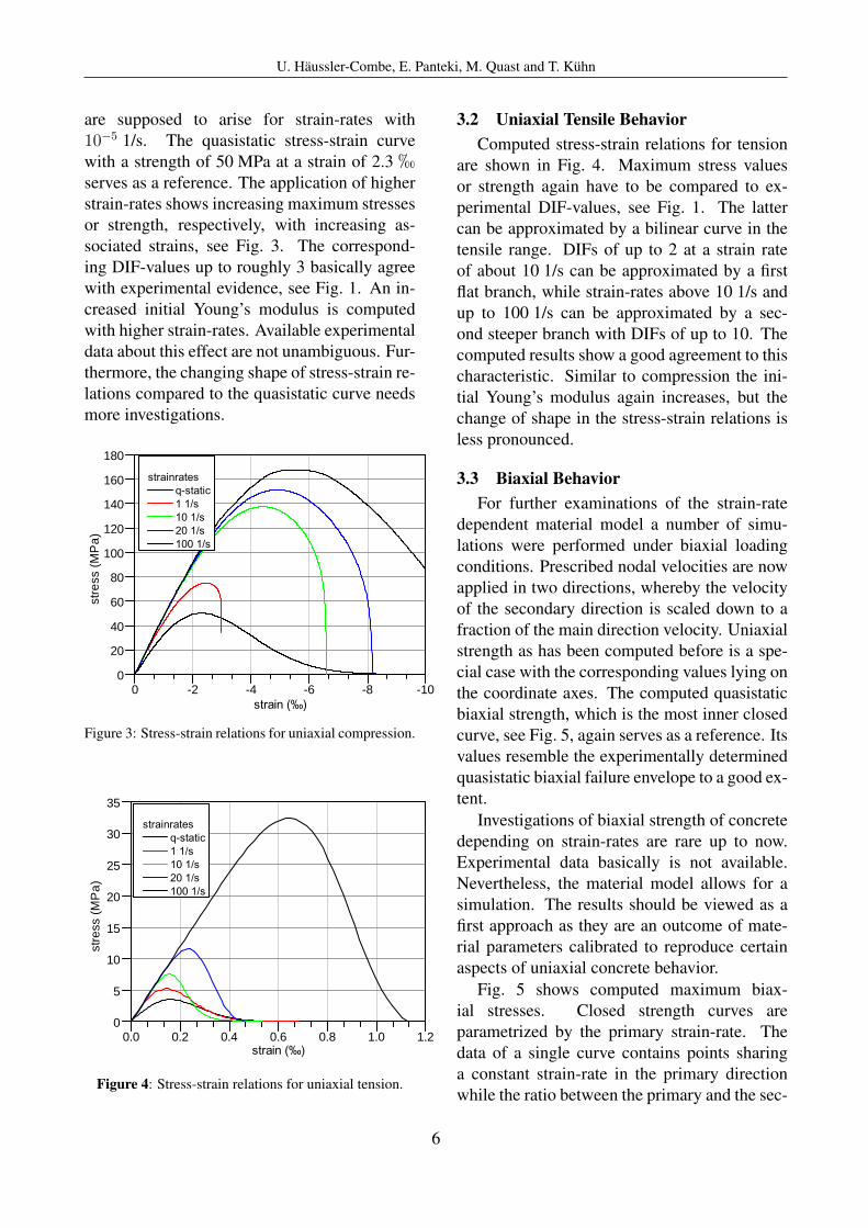
3.1 Uniaxial Compressive BehaviorThe resulting stress-strain relations in com-

pression are given in Fig. 3 depending on arange of strain-rates. Quasistatic stress states

5


are supposed to arise for strain-rates with10−5 1/s. The quasistatic stress-strain curvewith a strength of 50 MPa at a strain of 2.3 hserves as a reference. The application of higherstrain-rates shows increasing maximum stressesor strength, respectively, with increasing as-sociated strains, see Fig. 3. The correspond-ing DIF-values up to roughly 3 basically agreewith experimental evidence, see Fig. 1. An in-creased initial Young’s modulus is computedwith higher strain-rates. Available experimentaldata about this effect are not unambiguous. Fur-thermore, the changing shape of stress-strain re-lations compared to the quasistatic curve needsmore investigations.

0 - 2 - 4 - 6 - 8 - 1 00

2 04 06 08 0

1 0 01 2 01 4 01 6 01 8 0

stres

s (MP

a)

��

��

Figure 3: Stress-strain relations for uniaxial compression.

0 . 0 0 . 2 0 . 4 0 . 6 0 . 8 1 . 0 1 . 205

1 01 5

2 02 5

3 03 5

stres

s (MP

a)

��

��

Figure 4: Stress-strain relations for uniaxial tension.

3.2 Uniaxial Tensile BehaviorComputed stress-strain relations for tension

are shown in Fig. 4. Maximum stress valuesor strength again have to be compared to ex-perimental DIF-values, see Fig. 1. The lattercan be approximated by a bilinear curve in thetensile range. DIFs of up to 2 at a strain rateof about 10 1/s can be approximated by a firstflat branch, while strain-rates above 10 1/s andup to 100 1/s can be approximated by a sec-ond steeper branch with DIFs of up to 10. Thecomputed results show a good agreement to thischaracteristic. Similar to compression the ini-tial Young’s modulus again increases, but thechange of shape in the stress-strain relations isless pronounced.

3.3 Biaxial BehaviorFor further examinations of the strain-rate

dependent material model a number of simu-lations were performed under biaxial loadingconditions. Prescribed nodal velocities are nowapplied in two directions, whereby the velocityof the secondary direction is scaled down to afraction of the main direction velocity. Uniaxialstrength as has been computed before is a spe-cial case with the corresponding values lying onthe coordinate axes. The computed quasistaticbiaxial strength, which is the most inner closedcurve, see Fig. 5, again serves as a reference. Itsvalues resemble the experimentally determinedquasistatic biaxial failure envelope to a good ex-tent.

Investigations of biaxial strength of concretedepending on strain-rates are rare up to now.Experimental data basically is not available.Nevertheless, the material model allows for asimulation. The results should be viewed as afirst approach as they are an outcome of mate-rial parameters calibrated to reproduce certainaspects of uniaxial concrete behavior.

Fig. 5 shows computed maximum biax-ial stresses. Closed strength curves areparametrized by the primary strain-rate. Thedata of a single curve contains points sharinga constant strain-rate in the primary directionwhile the ratio between the primary and the sec-

6


ondary directions strain-rate varies between -1and 1 in steps of 0.1. Thus, the elements re-sultant strain-rate level differs for each calcula-tion run, limiting the direct comparability of theconnected curve points.

- 6 0 0 - 4 0 0 - 2 0 0 0

- 6 0 0

- 4 0 0

- 2 0 0

0

stres

s (MP

a)

s t r e s s ( M P a )

s t r a i n r a t e s q - s t a t i c 1 1 / s 1 0 1 / s 2 0 1 / s 1 0 0 1 / s

Figure 5: Biaxial dynamic failure curve.

It can be seen that biaxial strength increasemay by far exceed the uniaxial strength in-crease in the purely compressive range, espe-cially when both stress components have a sim-ilar level. This is not the case in the purely ten-sile range where uniaxial strength exceeds thebiaxial values as well for quasistatic as for highstrain-rate conditions.

The shape of the strength curves consider-ably differs in the area of combined tension andcompression compared to pure compression ortension. This is presumably related with in-terpolation effects between purely compressiveand purely tensile states according to the valueof the tension indicator, see Eq. (18). This ap-proach ensures on the one hand the continuity ofthe numerically determined biaxial failure en-velope and on the other hand the distinction be-tween moderate compressive and higher tensilestrength increase. Another point to consider isthe influence of the Poisson’s ratio, which is as-sumed as constant. Uniaxial extension for ex-

ample evokes tensile stresses in a first direc-tion while shortening occurs in the second andthird direction. Prescribed moderate compres-sive strain in the secondary direction counter-acts the shortening induced by the Poisson’seffect and cannot lead to compression as longas the tensile force dominates. A combinationof both interpolation and Poisson’s effects pre-sumably superposes to the special shape of thestrength curves in the upper corner of Fig. 5.

4 Biaxial Split-Hopkinson-Bar - Experi-ments

Biaxial experimental results were obtainedfrom a biaxial Split-Hopkinson-Bar (SHB) atthe Institute of Concrete Structures at the Tech-nische Universitat Dresden.

4.1 Experimental SetupThe test setup is basically identical to the one

shown in Fig. 6.

Figure 6: Split-Hopkinson-Bar basics.

It consists of a gas pressure accelerator withthe impactor and the specimen sandwiched be-tween the incident and the transmission bar,both made of aluminum and each with a diame-ter of 50 mm and a length 2.78 m . The gas pres-sure accelerator can be charged with up to 10bar compressed air and speed up the bronze im-pactor (d = 49.5 mm; l = 120 mm; m = 2040 g)to an impact velocity of 10 to 30 m/s. Thisimpact induces a compressive impulse, whichpropagates through the incident bar with a wavepropagation velocity of approx. 5000 m/s. Thecompressive impulse is measured in the middleof the incident bar by strain gauges.

7


At the end of the incident bar the impulsereaches the interface between aluminum andspecimen. Here the impulse is partly reflecteddue to the difference of impedance between alu-minum and concrete and partly transmitted intothe specimen. The reflected part propagates astension wave in reversed direction through theincident bar and is measured again in the mid-dle of the incident bar.

The part transmitted into the specimen gen-erally reaches the concrete strength and leads tofailure. Nevertheless, the transmitted part prop-agates through the specimen and might changeits amplitude and shape due to the nonlinearconcrete behavior. Further on, it is transmittedas compression wave into the transmission barwhere it is finally gauged again in the middle ofthe bar.

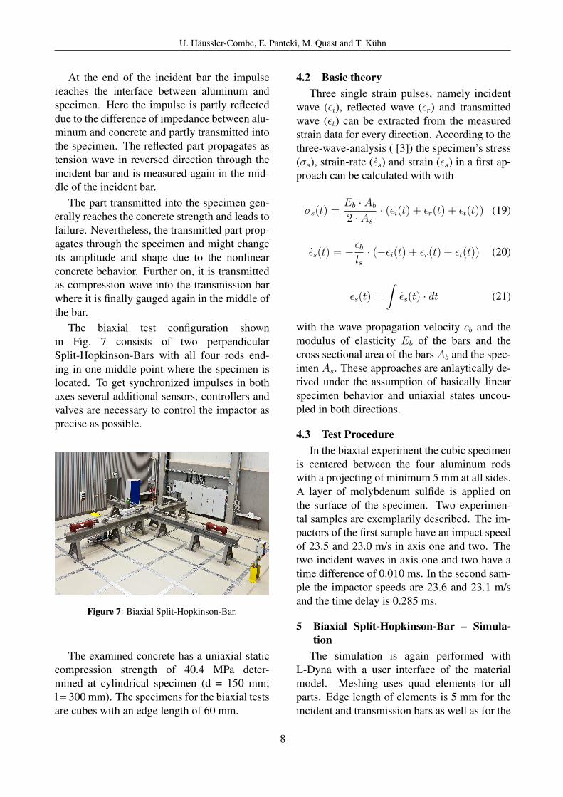
The biaxial test configuration shownin Fig. 7 consists of two perpendicularSplit-Hopkinson-Bars with all four rods end-ing in one middle point where the specimen islocated. To get synchronized impulses in bothaxes several additional sensors, controllers andvalves are necessary to control the impactor asprecise as possible.

Figure 7: Biaxial Split-Hopkinson-Bar.

The examined concrete has a uniaxial staticcompression strength of 40.4 MPa deter-mined at cylindrical specimen (d = 150 mm;l = 300 mm). The specimens for the biaxial testsare cubes with an edge length of 60 mm.

4.2 Basic theoryThree single strain pulses, namely incident

wave (εi), reflected wave (εr) and transmittedwave (εt) can be extracted from the measuredstrain data for every direction. According to thethree-wave-analysis ( [3]) the specimen’s stress(σs), strain-rate (εs) and strain (εs) in a first ap-proach can be calculated with with

σs(t) =Eb · Ab2 · As

· (εi(t) + εr(t) + εt(t)) (19)

εs(t) = −cbls· (−εi(t) + εr(t) + εt(t)) (20)

εs(t) =

∫εs(t) · dt (21)

with the wave propagation velocity cb and themodulus of elasticity Eb of the bars and thecross sectional area of the bars Ab and the spec-imen As. These approaches are anlaytically de-rived under the assumption of basically linearspecimen behavior and uniaxial states uncou-pled in both directions.

4.3 Test ProcedureIn the biaxial experiment the cubic specimen

is centered between the four aluminum rodswith a projecting of minimum 5 mm at all sides.A layer of molybdenum sulfide is applied onthe surface of the specimen. Two experimen-tal samples are exemplarily described. The im-pactors of the first sample have an impact speedof 23.5 and 23.0 m/s in axis one and two. Thetwo incident waves in axis one and two have atime difference of 0.010 ms. In the second sam-ple the impactor speeds are 23.6 and 23.1 m/sand the time delay is 0.285 ms.

5 Biaxial Split-Hopkinson-Bar – Simula-tion

The simulation is again performed withL-Dyna with a user interface of the materialmodel. Meshing uses quad elements for allparts. Edge length of elements is 5 mm for theincident and transmission bars as well as for the

8


impactor. A finer mesh was used for the spec-imen with an element size of approx. 2.5 mm.The material behavior of the impactor and thebars was assumed linear elastic, whereas for theconcrete specimen the nonlinear strain-rate de-pendent model was assumed. Simple contact al-gorithms were used allowing compressive loadsto be transferred between slave nodes and mas-ter segments. The friction coefficient was foundto be essential for the calculation results qualityand was set to 0.45 between the concrete andaluminum parts.

5.1 Model setupThe biaxial Split-Hopkinson-Bar dimen-

sions used for the study correspond to the ex-perimental setup described in Section 4. In allcases both impactors are given an initial ve-locity of 20 m/s, accounting for inaccuraciesin measurement. The experimentally measuredtime difference between the two waves is nu-merically incorporated as unequal distance be-tween the incident bar and the impactor for thetwo axes. In detail a distance of 0.2 respectively5.7 mm results in a delay of the time of 0.010respectively 0.285 ms of first contact betweenthe impactor and incident bar in the second axis.

5.2 Strain WavesFig. 8 and 9 compare the experimentally

measured with the numerically calculated strainwaves recorded at the strain gauge positions incase of a time delay of 0.010 ms. Both com-puted incident waves are in good accordancewith the experimental ones and the computedmaximal transmitted strain agrees with the ex-perimental data. The friction coefficient of 0.45between concrete and aluminum is of prime im-portance at this point, as it reduces the strainof the transmitted wave about 25 %, comparedto the case with friction coefficient set to 0.However, the reflected wave comes with differ-ing strain levels between experiment and mod-elling. A possible cause may be the prompt brit-tle failure of the first concrete elements in con-tact with the incident bar, forming a free endin terms of reflection. Another point on which

experiment and modelling do not coincide isthe wave propagation velocity in the specimen,which causes the numerical pulse to arrive ear-lier at the strain gauge position than the exper-imental one. Remarkable is also the fastly de-clining softening behaviour of concrete in caseof the computation results.

0 . 0 0 . 2 0 . 4 0 . 6 0 . 8- 3

- 2

- 1

0

1

2

3

��

��

t i m e ( m s )

i n c i d e n t b a r ( e x p . ) t r a n s m i t t e r b a r ( e x p . ) i n c i d e n t b a r ( n u m . ) t r a n s m i t t e r b a r ( n u m . )

Figure 8: Strain waves for 0.010 ms offset: first axis.

0 . 0 0 . 2 0 . 4 0 . 6 0 . 8- 3

- 2

- 1

0

1

2

3

��

��

t i m e ( m s )

i n c i d e n t b a r ( e x p . ) t r a n s m i t t e r b a r ( e x p . ) i n c i d e n t b a r ( n u m . ) t r a n s m i t t e r b a r ( n u m . )

Figure 9: Strain waves for 0.010 ms offset: second axis.

5.3 Global Results5.3.1 Stress-Strain Relations

Global stress-strain curves were determinedboth for the experiment and the calculationin accordance to the three-wave-analysis de-scribed in Section 4.2 They are shown in Fig. 10and in general indicate an accordance.

9


- 1 2 - 1 0 - 8 - 6 - 4 - 2 0- 1 5 0

- 1 0 0

- 5 0

0

��

stres

s (MP

a)

��

Figure 10: Experimental and numerical global results

5.3.2 Crack pattern

Fig. 11 compares the observed crack pat-terns with the spatial damage distribution in thespecimen and how they are influenced by thetime delay between the two pulses.

Figure 11: Crack pattern and damage distribution for atime delay of 0.010 ms (above) and 0.285 ms (below).

The upper scenario accounts for a time de-lay of 0.010 ms and the lower scenario for atime delay of 0.285 ms. In the first case theload causes cracks to form diagonally pointing

towards the middle of the adjacent aluminumbars, which arises in a rhombic pattern. Thebigger time difference, in contrast, leads cracksto open parallel to the first impulse direction.Fine cracks can also be detected right-angled tothat close to the load application point, probablybeing influenced by prevented lateral strain.

5.4 Local ResultsThe numerical simulation allows for a com-

prehensive evaluation of stresses and strains inevery element during the whole time. This leadsto local results which are discussed in the fol-lowing.

Figure 12: Triaxial principle stresses for perfectly biaxialloading condition.

5.4.1 Homogeneity

The following results are computed with theassumption of perfectly synchronized impulseswith equal amplitudes. This leads to identicalstresses in the z- and x-direction. Fig. 12 in-dicates the extremal stresses reached for rep-resentative elements during the whole loading

10


history. The upper part shows in-plane stresscomponents σzz (with the same stress compo-nents σxx), the lower part collateral stresses σyy.The x−z-plane spans the plane of the bar direc-tions. These results indicate that assumptionsabout homogeneity of stresses and plane stressstates are by far not fulfilled. This puts the ap-plicability of Eqs. (19) - (21) into perspective.

5.4.2 Variations of Local Results

Fig. 13 shows local stresses for the upperspecimen in Fig. 11. Each of the curves isrelated to a single element and indicates thein-plane stresses varying during the load his-tory.

- 3 0 0 - 2 0 0 - 1 0 0 0 1 0 0- 3 0 0

- 2 0 0

- 1 0 0

0

1 0 0 S X X - S Z Z S X X - M a x S Z Z - M a x S X X - M i n S Z Z - M i n

Stres

s SZZ

(MPa

)

S t r e s s S X X ( M P a )Figure 13: Local in-plane stress states varying with time.

The course of all stress states is shown ingrey. The elements with the minimal and max-imal values for each direction are highlightedwith colors. The shown results indicate a com-plex stress history with sequences of loading,unloading and reloading.

Fig. 14 shows the corresponding stress-strainrelations. Again elements with extremal val-ues are highlighted with colors and the partic-ular stress-strain relations can be considered asan indicator for failure and crack energy. Thecurves marked as SZZ-Min and SXX-Max re-main straight indicating an nearly linear elasticpath. SZZ-Min reaches a very high compressivestress level without failure which is probably

caused by the more pronounced biaxial or triax-ial stress state in the specific element. The bluecurve for SXX-Min shows failure in the com-pressive domain with large compressive strain.The red SZZ-Max curve instead shows a firstmaximum in compression with unloading andlater tensile failure at a lower tensile stress level.

- 3 0 - 2 0 - 1 0 0 1 0- 3 0 0

- 2 0 0

- 1 0 0

0

1 0 0

��

stres

s (MP

a)

��

Figure 14: Local stress-strain relations.

- 3 0 0 - 2 0 0 - 1 0 0 0 1 0 0- 3 0 0

- 2 0 0

- 1 0 0

0

1 0 0

��

Stres

s Z (M

Pa)

��

��

Figure 15: Local and global in-plane stresses.

Fig. 15 first of all shows local results of theelements with the extremal values in the ten-sile and compressive domain as single markers.Colors correspond to the previous figures indi-cating the different stress components. Differ-ent markers of the same color indicate differenttimes. Furthermore, global results derived using

11


Eqs. (19) - (21) are shown as curves or paths,respectively. Time varies along a path. The per-fectly biaxial path - no time delay - appears as astraight line whereas the local maxima are scat-tered. All global values or paths underestimatestresses compared to the locally observed ex-trema. The dark-grey curve indicates an aver-age of all considered elements, which is rela-tively close to the globally evaluated black one.This might confirm the global analysis proce-dure.

6 CONCLUSIONSExperimental and simulation results were

presented for concrete specimen exposed to bi-axial loading under high strain-rate conditions.The simulation model gives a reasonable agree-ment with the experiments with some detail dif-ferences. Evaluated states are triaxial, spatiallynot homogeneous and highly variable in timein case of the biaxial Split-Hopkinson-Bar. Bi-axial compressive strength by far seems to ex-ceed unaxial strength, much more pronouncedcompared to quasistatic behavior. All these phe-nomena still need more investigations.

7 ACKNOWLEDGEMENTThe project is funded by the German Fed-

eral Ministry of Economic Affairs and Energy(BMWi, project no. 1501483 and 1501486) onbasis of decision by the German Bundestag.

REFERENCES[1] P. Bischoff and S. Perry. Compressive be-

havior of concrete at high strain rates. Ma-terials and Structures, 24:425–450, 1991.

[2] CEB-FIP. Model Code for ConcreteStructures 2010. International Federationfor Structural Concrete (FIB), Lausanne,Switzerland, 2012.

[3] W. W. Chen and B. Song. Split Hopkinson(Kolsky) bar : design, testing and applica-tions. Springer, New York, NY ; Heidel-berg [u.a.], 2011.

[4] J. Eibl and B. Schmidt-Hurtienne. Strain-rate-sensitive constitutive law for con-

crete. Journal of Engineering Mechanics,125:1411–1420, 1999.

[5] E. J. Garboczi. Microstructure and trans-port properties of concrete. PerformanceCriteria for Concrete Durability, pages198–212, 1995.

[6] U. Haussler-Combe and J. Hartig. Formu-lation and numerical implementation of aconstitutive law for concrete with strain-based damage and plasticity. Interna-tional Journal of Non-Linear Mechanics,43:399–415, 2008.

[7] M. Jirasek. Nonlocal models for damageand fracture: comparison of approaches.International Journal of Solids and Struc-tures, 35:4133–4155, 1998.

[8] J. Lemaitre and R. Desmorat. Engineer-ing Damage Mechanics. Springer Verlag,Berlin, 2005.

[9] L. J. Malvar and C. A. Ross. Reviewof strain rate effects for concrete in ten-sion. ACI Materials Journal, 95:735–739,1998.

[10] L. E. Malvern. Introduction to theMechanics of a Continuous Medium.Prentice-Hall, Englewood Cliffs, New Jer-sey, 1. auflage edition, 1969.

[11] R. Peerlings, R. de Borst, W. Brekelmans,and J. de Vree. Gradient enhanced damagefor quasi-brittle materials. Int. J. Numer.Meth. Engng., 39:3391–3403, 1996.

[12] H. W. Reinhardt and J. Weerheijm. Tensilefracture of concrete at high loading ratestaking account of inertiaand crack velocityeffects. International Journal of Fracture,51:31–42, 1991.

[13] P. Rossi. A physical phenomenon whichcan explain the mechanical behaviour ofconcrete under high strain rates. Materi-als and Structures, 24:422–424, 1991.

12

Date post:	15-Feb-2019
Category:	Documents
Upload:	dinhnhan
View:	215 times
Download:	0 times

SIMULATION OF DYNAMIC FRACTURE OF CONCRETE WITH … · [email protected] Key words:...

Documents