SIMULATION OF PROGRESSIVE DAMAGE …publications.npl.co.uk/npl_web/pdf/matc20.pdf · ·...

NPL REPORT MATC(A)20

i

SIMULATION OF PROGRESSIVE DAMAGE FORMATION AND

FAILURE DURING THE LOADING OF CROSS-PLY COMPOSITES

L N McCartney NPL Materials Centre National Physical Laboratory Teddington, Middlesex United Kingdom, TW11 0LW

ABSTRACT

The objective of this report is to summarise the current status of theoretical models and associated software that are designed to predict damage initiation and growth in cross-ply laminates to the point of failure. For the case of static loading to failure, the damage modes that are modelled are ply cracking in the 90o plies of the laminate, fibre failure in the 0o plies (using Monte Carlo methods), and fibre/matrix debonding associated with fibre fractures. Biaxial loading of the laminate is permitted, and account is taken of the effect of thermal residual stresses at both the fibre/matrix and ply levels. The computer application for the prediction of failure during static loading is known as STRENGTH. For the case of the environmental degradation of cross-ply laminates arising from exposure to aggressive environments, the principal damage mode is fibre failure arising from the operation of stress-corrosion mechanisms at the fibre defects. Ply cracking is not included in this model. A computer application known as RESIDUAL has been developed that predicts the lifetime, and time dependence of residual strength, for a cross-ply laminate subject to biaxial loading and thermal residual stresses in an aggressive environment. Descriptions are given of the physical basis of the models, and the associated assumptions. In addition a description is given of how to operate the software, and sample numerical outputs are given. These results can be used to confirm that the software has been installed correctly, and act as a record of software performance (for quality assurance purposes) for the current versions of the applications STRENGTH and RESIDUAL. High quality model validation data (obtained in collaboration with others) are presented that relate to model performance at the fibre/matrix level, and ply cracking level. The validation of the application software is an on-going activity that has not reached a state of maturity. This is particularly true for strength and environmental degradation predictions, which are very complex phenomena that are very difficult to model reliably. The current versions of the applications are regarded as the first useful steps.


ii

© Crown copyright 2001 Reproduced by permission of Controller, HMSO ISSN 1473-2734 National Physical Laboratory Teddington, Middlesex, UK, TW11 0LW No extracts from this report may be reproduced without the prior written consent of the Managing Director, National Physical Laboratory; the source must be acknowledged. Approved on behalf of Managing Director, NPL, by Dr C Lea, Head of NPL Materials Centre.


iii

CONTENTS

1. Introduction.......................................................................................................................1

2. Description of the methodology .........................................................................................2 2.1 The application STRENGTH................................................................................2 2.2 The application RESIDUAL.................................................................................5

3. Representation of the cross-ply laminate.............................................................................5

4. Allocation of fibre strengths ...............................................................................................9 4.1 Weakest link fibre failure statistics........................................................................9 4.2 Use of the Weibull distribution function................................................................9

5. Load shedding .................................................................................................................10

6. Laminate failure criterion.................................................................................................10

7. Simulation procedure for STRENGTH and RESIDUAL...................................................11

8. Parameters used for the simulations..................................................................................11 8.1 Monte Carlo model data .....................................................................................11 8.2 Selection of length of fibre elements ...................................................................12 8.3 Parameters for the Weibull distribution ...............................................................12 8.4 Parameters for the micro-mechanical model........................................................13 8.5 Parameters for ply crack formation .....................................................................14 8.6 Parameters for environmental degradation...........................................................14

9. Operating the software on PCs .........................................................................................15

10. Samples of results ..........................................................................................................15 10.1 STRENGTH application...................................................................................15 10.2 Conclusions regarding the STRENGTH application ..........................................17 10.3 RESIDUAL application....................................................................................18 10.4 Conclusions regarding the RESIDUAL application ...........................................20

11. Validation of models......................................................................................................20

12. Overall conclusions........................................................................................................21

References ...........................................................................................................................22

Acknowledgement................................................................................................................23


iv

APPENDIX 1 : Input and output files for the application STRENGTH ..................................24

APPENDIX 2 : Input and output files for the application RESIDUAL ...................................28

APPENDIX 3 : Calculation procedure for STRENGTH application.......................................32

APPENDIX 4 : Monte Carlo simulation procedure for STRENGTH and RESIDUAL............33

APPENDIX 5 : Operation of the STRENGTH application....................................................34

APPENDIX 6 : Operation of the RESIDUAL application.....................................................37

APPENDIX 7 : Validation data for software used to predict undamaged ply properties from fibre and matrix data.........................................................................................40

APPENDIX 8 : Validation data for software used to predict damaged ply properties for various cross-ply laminates with non-uniform ply crack distributions .........................42

APPENDIX 9 : Experimental validation data for software used to predict damaged ply properties for various cross-ply laminates as a function of ply crack density ...............45

APPENDIX 10 : Validation data for stress transfer model that is the basis software used to predict damaged ply properties as a function of ply crack density ...........................48


1

1. Introduction The availability of reliable methods for predicting the failure of composite materials is perhaps one of the most important requirements when designing composite components and structures. The structural analysis of composite components often involves the use of finite element analysis (FEA) in order to take account of the complex geometries and material anisotropies that are encountered in practice. The failure of structures is predicted when a specific failure criterion is satisfied. For composite materials numerous failure criteria have been suggested and implemented as FEA codes. These criteria do not have a physical basis that can be related to the microstructure of composite materials. In particular, they do not take account of the fact that prior to catastrophic failure composite materials are subject to progressive microstructural damage in the form of ply cracking, delamination, fibre fracture and fibre/matrix debonding. The failure criteria (mainly stress based) are applied to stress fields that are estimated on the assumption that the material is undamaged. Thus, load transfer in structures arising from localised damage induced strain softening associated with stress concentrations is not taken into account. This phenomenon is largely responsible for composite materials out-performing expectations, which are based on zero-damage calculations. The use of failure models that account for damage induced strain-softening will lead to more efficient designs. Failure criteria for composite laminates have recently been assessed through a rigorous world-wide Exercise [1] that was designed to test various failure theories by comparing predictions with high quality experimental data. In the first part of the exercise (Part A), composite failure experts were asked to describe their methodology and apply it to predict the failure of a set of specified laminates. Each participant used the same laminate and materials data provided by the organisers. In Part A, participants were not provided with the experimental results relating to laminates used in the inter-comparison. The various predictions were then submitted to the organisers who then collated, compared and published the results (see [2]). The major finding was that in general there was a lack of agreement between the various failure criteria. Part B of the Exercise is currently in progress where participants now have had access to the experimental results, and they have had the opportunity of commenting on how well predictions based on their theories compare with the experimental results provided by the organisers of the Exercise. The results of the Part B phase of the inter-comparison are yet to be published. It is concluded from the results of Part A of the Exercise [2] that the prediction of the failure of composite laminates continues to be a very difficult unsolved problem. Future progress is likely to be possible only if steps are taken to base the prediction of laminate failure on the micromechanisms of damage that occur before the catastrophic failure event. As mentioned above, the damage modes that are likely to be important are fibre/matrix debonding, fibre fracture, ply cracking and delamination. One objective of this report is to describe progress that has been made in the development of a methodology that is designed to predict the progressive growth of some forms of damage, and the strength, of cross-ply laminates subject to biaxial tensile loading. A second objective is to describe progress that has been made with the development of a method to predict the lifetimes and time dependence of the residual strengths of cross-ply laminates whose properties are degraded by the influence of environmental factors. The attractiveness to Industry of any software system is dependent upon various factors. One concerns the provision of sample solutions that can be used to check the correct installation of software, and its operation. Appendices 1-6 provide such information relevant to the software applications STRENGTH and RESIDUAL that are the subject of this report. Perhaps the most


2

important is the thorough validation of the software by comparison of model performance with other models having equal or better quality, and with experimental results. A great deal of validation work has been undertaken both as part of the DTI Composites Performance and Design Programme (CPD), and through various informal collaborations with other research groups in the UK and abroad. The approach to validation is to establish model integrity to validate parts of the software progressively starting from theory and routines that apply at the fibre/matrix level, through to damage models at the ply and laminate levels. In Appendices 7-10 model validation data are given relating to the software routines that predict: • undamaged unidirectional laminate properties from fibre and matrix properties and the fibre

volume fraction, • the effects on laminate properties of non-uniform ply cracking, • the effects on the laminate thermoelastic constants, of ply cracking in the 90o plies, • the detailed stress and deformation distributions in a laminate with ply cracks.

2. Description of the methodology The methodology to be described in this report involves bringing together various mathematical models of specific composite damage modes for composites into two distinct computer applications that can predict the progressive formation of damage in a cross-ply laminate leading to failure. The objective here is not to provide details of the mechanics that have been used in the various models but to give a short description of the methodology and the software applications that have been developed. The first application STRENGTH is designed to predict the progressive property degradation and static strength of a cross-ply laminate subject to biaxial loading in the absence of environmental effects taking account of ply cracking, fibre fracture and fibre/matrix interface debonding. The software system integrates various software modules that can predict the various damage modes independently. The second application RESIDUAL is designed to predict the lifetime of a cross-ply laminate subject to biaxial loading in the presence of an environment that leads to a progressive degradation of properties and failure. The application is also designed to predict the time dependence of the residual strength of the laminate. Ply crack formation is not considered in this case. Both the applications STRENGTH and RESIDUAL take account of the effect of thermal residual stresses.

2.1 The application STRENGTH

The first damage mode that occurs in a multiple-ply cross-ply laminate loaded in tension is the occurrence of ply cracking in the 90o plies. This leads to a progressive loss in properties as the crack density increases. By making use of a stress transfer model for ply cracking [3, 4] all the thermoelastic constants of a laminate with ply cracks can be predicted accurately as a function of crack density. When considering ply crack formation in laminates one has to consider both the conditions for the initiation of ply damage in the form of small ply cracks, and the propagation of these ply cracks across the full width of the laminate. Ply damage initiation is extremely difficult to predict due to the operation of various types of localised damage such as fibre/matrix debonds, coalescence of debonds into ply defects, and the growth of these defects into fully developed ply defects that can be modelled at the continuum level rather than at the fibre/matrix level.


3

Defect size

Str

ess

for

pro

pag

atio

n Unstable growth

Stable growth

Design limit

Fibre/matrix debonds

Thick plies

Long plycracks

Thin plies

Fig.1 : Schematic diagram illustrating the basis of the design limit for ply cracking.

It is useful to refer to Fig.1 when discussing the initiation and propagation stages of ply crack formation. Consider first of all the case of stable ply crack growth following initiation (lower curve). Once a ply defect has formed from localised fibre/matrix debonds or other small defects an increasing stress is needed in order for the ply defect to grow in size. Eventually a ply crack is formed that behaves as a long crack where the energy release rate is independent of ply crack length. The stress needed for steady state ply crack growth is then the stress needed to grow the ply crack across the full width of the laminate. The limiting ply cracking stress in this case is then clearly the relevant stress for use in a design procedure, as any stress less than this value will not generate fully developed ply cracks. Such stable ply crack growth is not, however, observed in practice. This leads on the other situation that is believed to occur in practice. For this case (upper curve) the stress needed to initiate a ply defect is larger than the stress needed for steady state ply crack growth. Thus once a ply defect grows to a size large enough for ply crack growth to occur, the growth is unstable and a fully developed ply crack instantaneously forms. When the 90o ply thickness is relatively large the initiation stress is likely to be larger than the steady state propagation stress, but when the 90o plies are thin, ply crack growth is expected to be controlled by the steady state limiting ply-cracking stress. Thus for the unstable ply crack growth situation that is expected in practice, the steady state ply cracking limit used as the design limit is expected to be an accurate estimate only if the 90o plies are thin enough (i.e. of the order of thickness of the 0o plies). For thicker plies the steady state design limit will provide lower bound (and thus safe) estimates for the ply cracking stress. Using energy methods [4, 5, 6], predicted values of the thermoelastic constants for damaged laminates can be used to predict the progressive formation of ply cracks during tensile loading. The software system PREDICT has been developed to deal with this type of damage formation for both cross-ply laminates and general symmetric laminates, and is being commercially exploited by its inclusion as one module for the UK Integrated Composite Design Toolset, a commercially supported software system being developed jointly by DERA (Managers of project), AEA Technology and NPL. The Toolset is being commercialised by SER Systems Ltd (formerly known as PAFEC). Predictions can be made using fibre/matrix properties or


4

using experimentally measured ply properties. The methods of analysis for ply crack formation provided by PREDICT do not provide a methodology for predicting the failure of a laminate during static testing. To overcome this limitation of the ply-cracking model, use has been made of a recently developed Monte Carlo method [7] for predicting the tensile strength of unidirectional (UD) fibre reinforced composites. The approach divides a representative part of the UD composite into fibre/matrix cells of small size (up to 1mm in length) each containing just one fibre/matrix element. The fibres in each cell have statistically distributed fibre strengths based on the Weibull distribution. In the application STRENGTH the Monte Carlo model is applied only to the 0o plies of the laminate. The original Monte Carlo model known as MONTE, designed for a uniaxial loading case, has been modified to account approximately for the triaxial stress state that arises in the 0o plies of a cross-ply laminate when loaded in tension and subject to thermal residual stresses resulting from thermal expansion mismatch effects between plies. The application MONTE simulates the effects of progressive fibre failure on the axial modulus of a UD composite up to the point of catastrophic failure. Fibre failures can have a significant effect on the effective axial modulus of the 0o plies particularly when the catastrophic failure event is approached, especially for glass fibre composites and moderate fibre volume fractions. An important aspect of the Monte Carlo modelling is the inclusion of fibre/matrix debonding that arises when fibres break. The theoretical basis of the interfacial debonding model is given in reference [8]. Fibre/matrix debonding is modelled using a software application known as TAUMOD that predicts the effective axial modulus of a fibre/matrix element having a fibre fracture as a function of the axial stress. Fibre/matrix debonding is assumed to be characterised by a fixed value for the interfacial shear stress t which can represent either a uniform frictional interfacial stress associated with debonding or a uniform shear stress arising from interfacial plasticity (shear yielding). Interfacial debonding leads to changes in stress transfer between fibre and matrix, and to further changes in the effective modulus of the 0o plies. These changes in the effective modulus of the 0o plies arising from fibre fracture events can have an influence on ply crack formation in the laminate. It should be noted that the stress transfer model used to predict interface debonding during the Monte Carlo simulation does not involve the fracture energy for debonding. This is a limitation of the current model which can be overcome only by the implementation of a stress transfer model that can represent the stress field more accurately. This can be achieved by adopting a layer refinement technique where the cylindrical elements representing the fibre and matrix are subdivided into concentric sub-elements enabling more realistic modelling of the radial dependence of the stress field, particularly the radial stress that describes the singularity of the stress field at the debond tip. The presence of this singularity (or an attempt to model it) is essential if interfacial fracture is to be correctly modelled through the use of an energy release rate. A stress transfer model has been investigated in detail in Project CPD3 on Interface Characterisation and Behaviour, and found to need more development that will be attempted in the Measurements for Materials Systems Programme (Project 3 on Modelling Damage in Multi-layer Systems). When used within a cross-ply laminate in which ply crack formation, fibre fracture and interfacial fibre/matrix debonding are occurring, the various software applications (PREDICT, MONTE and TAUMOD) have to be used interactively within computer application STRENGTH. Graphical output (FORTRAN based and thus only of an adequate quality) is included in the application. It is proposed that the STRENGTH module, when fully mature, should be included in the UK Composites Design Toolset.


5

2.2 The application RESIDUAL

The second application to be discussed concerns the failure of a cross-ply laminate that is subject to degradation arising from the influence of an aggressive environment. As laminate strength is dominated by the performance of the fibres, it is assumed that the effect of the environment on matrix properties can be neglected. Also, the application RESIDUAL does not account for ply crack formation. The degradation mechanism that is assumed to operate concerns the time dependence of fibre strengths arising from the progressive growth of fibre defects (expected mainly for glass fibres). The model predicts fibre defect growth on the basis of the coupling of a defect growth law with Weibull statistics where fibre strength is related to defect size using the Griffith fracture criterion. The environment has the effect of causing fibre defect growth at a rate that depends on both the current size of the defect and the local fibre stress. Defect growth occurs under the influence of fixed loads applied to the fibres, and can be modified if the load applied to the fibres is cyclic [9]. The strengths of the fibres thus progressively degrade leading to progressive fibre fractures and the eventual failure of the laminate. The methodology for the prediction of fibre degradation in unidirectional composites has been described in reference [10] for the special case where the environment has degraded interface properties to the extent that the fibres and matrix act independently. For the application RESIDUAL, the same type of fibre degradation is assumed, but the interface properties are assumed to be maintained following environmental exposure (although they might be degraded). Monte Carlo methodology [7] has again to be applied in conjunction with the modelling of interface debonding or shear yielding [8] that arises when fibres break. When the Monte Carlo and interface debonding models are applied to the degradation of the cross-ply laminate, account is taken of the degradation of the macroscopic properties of the 0o-plies. This can affect the load that is carried by the 0o-plies throughout the simulation because of stress transfer between the 0o and 90o plies of the laminate. The application RESIDUAL has been configured so that it is possible for predictions to be made of the laminate lifetime where the load applied to the laminate is held fixed throughout the simulation. In addition the application can be used to predict the residual strength of the laminate after loading at fixed applied stress for any fixed length of time that is less than the laminate’s lifetime. Graphical output (FORTRAN based and thus only of an adequate quality) is included in the application. It is again proposed that the RESIDUAL module, when mature, should be included in the UK Composites Design Toolset. One objective of this of this report is to describe how the software applications STRENGTH and RESIDUAL are used, and to provide the results of predictions that illustrate the principal characteristics of the applications.

3. Representation of the cross-ply laminate Fig.2 shows the edge view of a simple cross-ply laminate that is representative of more complex multiple-layer laminates that can be handled by the application STRENGTH (and by RESIDUAL, although predictions are not affected by the laminate lay-up in this case as ply cracking is not considered).


6

0o 0o90o

Fig.2 : Schematic diagram of the edge view of a cross-ply laminate with ply cracks and the

representative fibre/matrix cell (containing a broken fibre) of a 0o ply. During loading the first damage mode encountered is the progressive formation of ply cracks in the 90o layers as shown in Fig.2 Also shown is an expanded view of the fibre and matrix region (to be referred to as a fibre/matrix cell) that is associated with a single fibre fracture in one of the 0o plies of the laminate. This region is a representative volume element of the 0o ply and any fibre element may either be broken (as shown in Fig.2) or intact. The representative cell is selected to be a concentric cylinder geometry having the same fibre volume fraction as the fibres in the 0o plies. In order to predict the formation and effect of the ply cracks on the properties of the cross-ply laminate, the ply cracking model STRENGTH distributes on potential ply crack formation sites a set of randomly generated fracture energies for ply cracking. These values are taken from a normal distribution that is uniquely described by its mean fracture energy and standard deviation. The application STRENGTH uses Monte Carlo modelling in order to simulate progressive fibre fracture and failure as described in [7]. The new application RESIDUAL, which also uses Monte Carlo modelling of fibre failure, neglects ply crack formation but includes time dependent fibre degradation as described in [9].


7

Fig.3 : Schematic diagram of a representative element of a 0o ply in a cross-ply laminate. Fig.3 shows a schematic diagram of a representative part of the 0o plies in a cross-ply laminate where L rectangular layers of fibre/matrix cells having the same thickness δ are stacked vertically. The thickness of each layer is to be small enough for there to be at most just one fibre fracture in each element, and large enough for the stress transfer length (including fibre/matrix debonding zone) to be included entirely within the layer for all states of loading. This situation is not ideal, but required in order to avoid excessive computation times. The pace of processor speed increase is such that high performance PCs will enable more layers to be included in simulations without incurring unacceptably large execution times. Each layer is divided into an array (i, j) of individual fibre/matrix cells, each containing just one fibre element of the composite together with the neighbouring associated matrix. The fibres are assumed to be hexagonally packed on 2MN points of a rectangular 2M x 2N array. The strength of the fibre elements in each of the fibre/matrix cells is assumed to be statistically distributed according to a two-parameter Weibull distribution [11]. Progressive fibre failure in the 0o plies of the laminate is predicted using a Monte Carlo simulation technique [7] and its associated computer application MONTE. An issue worth emphasising concerns the role of fibre stress and strain during fibre failure. For a single fibre test the fibre stress and strain are both uniaxial with the result that the failure condition for the fibre can be characterised either by its strength or by its failure strain, which is obviously related to the strength through the fibre modulus. Within a composite, however, the


8

stress and strain states will not in general be uniaxial, leading to a choice having to be made regarding whether the axial stress or strain in a fibre governs its failure. In this report and the associated software it has been assumed that the fibre fails when its axial stress has the value of the local fibre strength in keeping with the traditional approach. It would be useful to consider also the case when the fibre axial strain controls fibre failure. While this is uncommon when predicting the failure of fibres in a composite, it is perhaps more justified from a physical point of view as it is the presence of fibre defects that determine the fibre strength whose behaviour would be strain controlled if one regarded fibre failure as the breakdown of cohesion. It would be very useful to compare the effect of the fibre failure criterion on predictions of composite strength. The application TAUMOD concerns the prediction of stress transfer and fibre/matrix debonding arising from fibre fracture in just one fibre/matrix cell. The Monte Carlo simulation uses directly the fibre/matrix stress transfer model TAUMOD in order to be able to predict the load sharing that occurs when the load carried by a breaking fibre is transferred to neighbouring intact fibre/matrix cells. TAUMOD estimates the change of stress state in the fibre/matrix cell that arises when a fibre breaks, including when subsequent local stress increases occur due to the failure of neighbouring intact fibres and to applied load increases. The current model assumes that the load carried by the matrix is small in comparison to that carried by fibres so that a matrix failure criterion does not need to be imposed. It turns out that this assumption does not lead to realistic stress-strain response of the laminate near the failure point (to be discussed later). Further developments are needed to include a matrix failure criterion in the model, such as a critical strain criterion. An important feature of the layered structure for the fibre/matrix cell arrangement is that cyclic edge conditions can easily be implemented in the three principal directions which are orthogonal. This is an essential requirement when simulating composite behaviour because load redistribution must be considered whenever a fibre fails. By using cyclic edge conditions there is no need to investigate whether a fibre/matrix cell is at or near a free surface or corner where modified load sharing rules would otherwise have to be applied. As the cyclic edge conditions are applied in three orthogonal directions the simulation will be representative of the internal regions of a 0o ply. This procedure maps the effects of events at locations lying beyond the region of simulation into the region that is under consideration. The simulation is thus expected to be representative of the behaviour of any 0o ply in the cross-ply laminate. It should be noted that the use of periodic edge conditions in the Monte Carlo simulation, such that the damage pattern in the simulated region is mapped into much larger regions, means that edge effects associated with free boundaries in unidirectional composites cannot be modelled. Stress transfer between a broken fibre in this region, and neighbouring surviving fibres, will be affected by the presence of the free surface of the composite. This cannot be modelled adequately at present as such modelling would require the inclusion of a very large number of fibres in the simulation. The effects of such edge phenomena are expected to be small, unless the free surface is subject to fibre damage because of handling etc. Such damage would have to be included in the model as pre-existing fibre fractures located in a region representative of that near the free surface.


9

4. Allocation of fibre strengths

4.1 Weakest link fibre failure statistics The statistical failure of fibres in the composite is modelled using weakest link methods [12]. It is well known that the strength of a fibre depends upon the fibre length. For the composite failure simulation under discussion, this presents significant problems as the length of fibre δ involved in each fibre element of the simulation may be small. It is clearly not possible to carry out reliable experiments on fibres of small lengths so that some type of extrapolation technique is needed. In the simulations to be reported here δ is selected to be 1 mm ensuring that all fibre/matrix debonding is contained within the fibre/matrix cell in which a fibre fracture occurs. Recent work has indicated that the value of δ can be reduced, but computation limitations lead to shorter sample lengths and the need to adopt some form of scaling in order to take account of the size effect.

4.2 Use of the Weibull distribution function

The Weibull distribution [11] function is frequently used to model fibre strength data. The Weibull distribution has the important property, not often realised, that it is one of three limiting distributions predicted by extreme value statistics [13]. In fact it is the only limiting distribution that is defined for positive values of the statistical variable. As strength is always positive, it is appropriate to make use of the Weibull distribution to model the statistical variability of fibre strength. Its use leads to a reliable method of extrapolation of experimental data for long fibre lengths to the short lengths needed by the simulation. The other two limiting distributions predicted by extreme value theory involve both positive and negative values of the statistical variable which would certainly not be appropriate for modelling fibre strength measurements. The cumulative Weibull strength distribution for fibres of length δ may be written

PF o( ) = 1 exp[ ( / ) ] ,mσ δ σ σ− − (1)

where δ is the length of fibre element and where m is the Weibull modulus and σo is a

scaling parameter having the dimensions of stress. Strictly speaking δ is dimensionless, being the ratio of the fibre element length to the ‘unit’ length (here selected to be 1 mm) that is the basis of the representation (1). The mean and variance of the distribution (1) are given by

mean = 11

m ,/σ δo

m− +FHG

IKJ

1 Γ (2)

variance = 12

m1

1

m ,/ 2σ δo

m2 2− +FHG

IKJ − +F

HGIKJ

LNM

OQPΓ Γ (3)

where Γ(x) is the Gamma function. The next stage is to construct a sequence of fibre strength levels that belong to the selected Weibull distribution. The method used is to generate a sequence of random numbers xk, k = 1....n lying in the range 0 ≤ x < 1 such that n is the total number of fibre elements in the simulation. Values generated by this procedure are allocated in sequence to each fibre element


10

of the system. One problem that arises from this procedure is that very large or rather small fibre strengths can be generated which are not really encountered in practice. To avoid the occurrence of this, if a fibre strength generated by the procedure exceeds its mean value by twice the standard deviation, then the value is rejected and a new value is calculated. In addition, if the fibre strength is smaller than one tenth of the standard deviation, then the fibre strength is again rejected and a new value is calculated. The bias introduced into the simulation is expected to be much smaller than errors arising from approximations that have to be made. On regarding the sequence xk as representing values of the cumulative failure probability PF(σ), it is easily shown from (1) that the required random strength levels are given by

sx

nk ok

= 1

ln1

1 , k = 1... .

1/m

σδ −LNM

OQP

(4)

It should be noted there is some uncertainty regarding the relevance of values of m and σo obtained from single fibre tests, to their application to fibres that are embedded in a composite. No reliable technique has been developed that enables the in-situ values of these parameters to be obtained, despite various claims in the literature.

5. Load shedding The next stage is to discuss how the load carried by failing fibre/matrix cells is transferred to neighbouring fibre/matrix cells in the 0o plies of the composite. It is assumed that the load shed by a failing fibre/matrix cell is shared (in a manner described in [7]) between the failing fibre/matrix cell and active neighbours in the same layer as the fibre/matrix cell that has failed. The active neighbours of the failing cell are those lying within the nearest neighbour hexagonal ring of fibres that contains at least one surviving fibre/matrix cell. It is emphasised that load is shed to failed fibre/matrix cells where the matrix has been assumed to be always intact. As mentioned above, it is recommended that a critical matrix strain is assumed at which the matrix can fail leading to the need to shed further load to surrounding fibre/matrix cells. If the fibre elements in all the nearest neighbour cells have failed then load is assumed to be transferred to all fibre/matrix cells enclosed by the next ring of nearest neighbours, and so on. This procedure specifies that the active load-sharing region is a small part of the layer containing the failed fibre. If just one fibre/matrix cell in the composite remains intact, albeit in an unstable situation, then its nearest surviving neighbour is its image lying beyond the representative volume element used in the simulation. At least one of these fibre/matrix cells will be detected by the use of cyclic boundary conditions and the complete failure of a layer is thus possible. It should be noted that load sharing confined to a single layer is reasonable only if the length δ of each elemental layer is greater than or equal to the maximum expected stress transfer length (often called ineffective length) associated with a single fibre break.

6. Laminate failure criterion The cross-ply laminate is considered to have failed catastrophically when the effective stress in the 0o plies of the laminate reaches the catastrophic failure stress predicted by the Monte Carlo simulation, taking full account of the effects of biaxial stress states and thermal residual stresses. When considering whether layer r in the representative region of the 0o plies of the laminate has failed, the fibre/matrix cell at location (i, j) is regarded as having failed if a fibre element failure can be detected at location (i, j) in layers r - h, r - h + 1, .... r , .... r + h - 1, r + h ,


11

where h ≥ 0 is a parameter that is selected and held fixed throughout the simulation. Assessing whether layer r has failed according to this failure criterion is particularly simple as the state of each fibre element is stored in a three dimensional logical array where failed fibre elements are denoted by ‘false’. Changing the value of h would be expected to vary the degree of fibre pull-out for cases where δ is small enough (i.e. much smaller than the value of 1 mm that is currently used).

7. Simulation procedure for STRENGTH and RESIDUAL The STRENGTH application for the simulation of progressive damage formation during the static testing of cross-ply laminates is described by distinct calculation stages described in Appendix 3. The RESIDUAL application for the simulation of progressive damage formation during the static testing of cross-ply laminates subject to environmental degradation follows the same Stages 1-6 given in Appendix 3 for the STRENGTH application. No ply cracking is allowed in RESIDUAL so that Stages 7 and 8 of the STRENGTH application are not needed. The Monte Carlo modelling in RESIDUAL, when predicting laminate lifetime, is very different to that used in STRENGTH. First of all the stress applied to the laminate is held fixed. The effective axial stress arising in the 0o-plies does however change because of stress transfer between the 0o and 90o-plies arising from axial stiffness loss in the 0o-plies that is caused by progressive fibre fracture in these plies. The simulation makes use of a fibre defect growth law relating the defect growth rate (da/dt where a is the defect size) to the effective stress intensity factor for the defect which has the empirical form

da

dtKn= Λ , (5)

where Λ and n are material constants. During any stage of the Monte Carlo simulation the current strength of each fibre element is calculated on integrating (5), and fibre elements are allowed to fail when their strength has declined to the current value of the fibre stress. Load sharing is then performed as in the STRENGTH application. This procedure is repeated until the 0o-plies can no longer support any load. The time at which this occurs determines the lifetime of the laminate. The software has also been developed so that can predict the time-dependence of the residual strength of the laminate. For both the applications STRENGTH and RESIDUAL the Monte Carlo simulation of progressive fibre fracture in the 0o plies of the laminate follows the procedure described in Appendix 4.

8. Parameters used for the simulations In this report preliminary predictions are made that are based on some high quality materials data that was used for the international failure prediction exercise [1]. A self consistent set of data was provided by the authors covering most of the materials parameters needed by the applications STRENGTH and RESIDUAL. Data that is needed here but not specified in [1] has been obtained from the literature.

8.1 Monte Carlo model data

It is useful to list the parameters that need to be specified before carrying out Monte Carlo simulations, namely


12

M, N parameters defining number of fibres (2MN) in the composite sample, L number of layers of fibre elements of length δ stacked vertically, H parameter characterising the number of layers considered when assessing failure of the 0o plies (total number is 2H + 1). The values used for preliminary simulations that should not have long execution times are M = N = 15, L = 1 and H = 0 so that there will be minimal fibre pull-out.

8.2 Selection of length of fibre elements The length δ of the fibre elements in the system is determined by the nature of stress transfer between fibre and matrix in the neighbourhood of an isolated fibre break. The value of δ� must be large enough for it to include all fibre/matrix debonding that occurs during loading following the failure of a fibre. One value will be investigated here namely δ �= 1 mm that leads to tolerable computation times (< 5 min.).

8.3 Parameters for the Weibull distribution

The remaining parameters that need to be specified relate to the allocation of fibre strengths using the Weibull distribution. These parameters are: m the dimensionless shape parameter for the distribution, σo a normalising parameter having the dimensions of stress. These parameters must relate to fibre elements of length δ used in the simulation that is assumed to be 1 mm. Experimental measurements from single fibre tests are not suitable as input values. A useful method of determining the appropriate parameter values is to investigate possible values from mean fibre strength measurements. For example, for one of the carbon fibres (AS4) used in the international failure prediction exercise [1] the strength in tension was specified to be 3.35 GPa, but no information was given regarding the statistical variability of fibre strength. The following Weibull parameters result when the Weibull distribution for various values of m is fitted to the specified mean strength for fibres assumed to have length 50 mm : m = 8 σo = 5.801 GPa

m = 6 σo = 6.931 GPa m = 4 σo = 9.828 GPa .

For Silenka E-glass fibres used in the international failure prediction exercise [1] the strength in tension was specified to be 2.15 GPa, but again no information was given regarding the statistical variability of fibre strength. The following Weibull parameters (for fibres of length of 1 mm) result when the Weibull distribution for various values of m is fitted to the specified mean strength of fibres having the various lengths specified in brackets :


13

m = 10 σo = 3.342 GPa ( 50 mm length) m = 8 σo = 4.0598 GPa (100 mm length) m = 8 σo = 3.723 GPa ( 50 mm length) m = 8 σo = 2.284 GPa ( 1 mm length) m = 6 σo = 4.993 GPa (100 mm length) m = 5 σo = 5.121 GPa ( 50 mm length) m = 4 σo = 7.501 GPa (100 mm length)

8.4 Parameters for the micro-mechanical model

In order to test the methodology and the associated computer software, it is necessary to select values for fibre, matrix and interface properties that are required by the micromechanical model of stress transfer. One material to be used for the micromechanical model is a carbon fibre (AS4) reinforced epoxy (3501-6) composite where the radius of the fibres is 3.5 microns, the volume fraction of fibres is taken as 0.6, and the stress-free temperature is such that ∆T = -157oC. The parameter ∆T T T= − 0 where T is the simulation temperature and T0 is the stress-free temperature for the laminate. The properties for the carbon fibre reinforced epoxy are : Fibre Matrix

EA (GPa) 225.0 4.2 ET (GPa) 15.0 4.2 m A (GPa) 15.0 1.56716 n A 0.2 0.34 n T 0.0714 0.34 a A (/oC x 106) - 0.5 45.0 a T(/oC x 106) 15.0 45.0

Another material to be used for the micromechanical model is a Silenka E-glass fibre reinforced epoxy (MY750/HY917/DY063)) composite where the radius of the fibres is assumed to be 8 microns, the volume fraction of fibres is taken as 0.6, and the stress-free temperature is such that ∆T = -100oC. The properties for the E-glass fibre reinforced epoxy are : Fibre Matrix

EA (GPa) 74.0 3.35 ET (GPa) 74.0 3.35 m A (GPa) 30.83333 1.24074 n A 0.2 0.35 n T 0.2 0.35 a A (/oC x 106) 4.9 58.0 a T(/oC x 106) 4.9 58.0


14

Fibre/matrix debonding is modelled by the use of the constant interfacial shear stress model where the critical interfacial shear stress τ characterises interface debonding, or shear yielding. The value selected for the investigation of the feasibility of the simulation technique is τ = 50 MPa.

8.5 Parameters for ply crack formation

Ply crack formation in the cross-ply laminate model is governed by the distribution of fracture energies for ply cracking. A normal distribution is assumed that is fully characterised by two parameters: the mean fracture energy 2γ for ply cracking and the standard deviation. It follows from the data given in [1] for strain energy release rate for cracking in 90o ply material alone that the mean fracture energy for ply cracking 2γ in carbon fibre (AS4) reinforced epoxy is 220 J/m2 while that for Silenka E-glass reinforced epoxy is 165 J/m2. The standard deviation is not specified but it is assumed here to be 15% of the mean fracture energy values. The number of potential crack formation sites is taken as 200 for a length 50 mm of laminate.

8.6 Parameters for environmental degradation

The specification of the parameters Λ and n appearing in the fibre defect growth law (5) is particularly difficult. The parameter Λ does not need to be specified provided that the simulation is conducted using a normalised time scale that is dimensionless. Its value is best determined by fitting model predictions to experimental results, rather than attempting to develop special methods for its direct measurement. For simulations there is, however, no loss of generality by selecting the value Λ = 1. The normalised times used in the simulation are then defined by

t K y E tIcn

f' = −1

22 2 2Λ , (6)

where t is the elapsed time in seconds, Ef is the fibre axial modulus, KIc is the effective fracture toughness for defects in the fibre, and y is a dimensionless parameter such that the stress intensity factor for the fibre defect is given by

K y af= σ . (7) The exponent n in the growth law (5) is also unknown and is likely to be material dependent. Extreme values of n = 3 and n = 15 will be assumed for GRP when carrying out preliminary predictions. N.B. In (6) an improvement would be to replace the factor E f

2 by σo2 so that the normalised

time is given by

t K y t tIcn

o' = =−1

22 2 2Λ σ η , (8)

which then corresponds to the normalised time used in the model where interface bonding is neglected. This modification will be made in the next version of the software.


15

9. Operating the software on PCs The software, written in FORTRAN 77, can be implemented on any PC provided that certain files are placed in specific directories on the C: drive. It is suggested that all executable files are placed in the directory C:\PREDICT which has subdirectories STRENGTH and RESIDUAL for the specific distinct applications. In addition it is necessary to create a directory C:\PREDAPP in which data files are placed, both to control the software, and to store data needed during the simulations. Output files of useful results generated during the simulation are stored as text files in the appropriate application directory. These are easily exported to Excel spreadsheets if needed (using comma rather than space as the delimiter). In-built within the software are methods of showing graphical output (not of high quality but adequate to assess the performance of the models) which can be printed. Both applications require fibre and matrix data which must be stored in the directory C:\PREDAPP using the filenames FIBRE.dat and MATRIX.dat (see Appendix 1 for file format). All software is run from various executable files, and data files. In addition, it is necessary to locate the FORTRAN library file SALFLIBC.dll (1.36 Mbytes) in the standard directory of the PC having the name C:\WINDOWS\SYSTEM. Descriptions of the operation of the applications STRENGTH and RESIDUAL are given respectively in Appendices 5 & 6. Some of the description that is common to both applications has been repeated to assist those who are using just one of the applications.

10. Samples of results

10.1 STRENGTH application

The data files given in Appendix 1 indicate the default control values that have been set for the STRENGTH simulation. Their values are easily reset by editing the appropriate file in the STRENGTH directory. Figs.4-6 are easily constructed from the output data given in the files XRNDPLT1.txt and XRNDPLT2.txt. The results plotted do not correspond to the data used in Appendix 1 as many more ply cracking sites (1000) have been used, and the loading is uniaxial, whereas the example in Appendix 1 is for 200 ply cracking sites and biaxial loading. It should be noted that, in the interests of having relatively quick simulations only one layer has been included in the Monte Carlo model for the 0o plies.


16

Fig.4 : Predicted stress-strain behaviour for a CFRP cross-ply laminate showing the minimal

effect on stress-strain response of including fibre fractures in the simulation.

Fig.5 : Predicted ply crack growth behaviour for a CFRP cross-ply laminate showing the minimal effect of including fibre fractures in the simulation.

Stress-strain behaviour

0

0.2

0.4

0.6

0.8

1

1.2

1.4

0 0.5 1 1.5 2 2.5

Axial strain %

Axi

al s

tres

s (G

Pa)

No fibre fracture

Fibre fracture

Growth of ply cracks during axial loading

0

0.5

1

1.5

2

0 0.2 0.4 0.6 0.8 1 1.2 1.4

Axial stress (GPa)

Cra

ck d

ensi

ty (

/mm

)

No fibre fracture

Fibre fracture


17

Fig.6 : Predicted modulus degradation behaviour for a CFRP cross-ply laminate showing the

effect of including fibre fractures in the simulation.

10.2 Conclusions regarding the STRENGTH application

While a good start has been made developing methods for predicting the damage growth and failure in cross-ply laminates subject to biaxial loading and thermal residual stresses, the model needs further refinement before it can be regarded as being a mature design tool. It has been possible to integrate models and software that connect interface modelling associated with fibre breaks to ply cracking models for cross-ply laminates. As already mentioned, the failure of the matrix has not been adequately modelled leading to unrealistic modulus degradations and failure strains at large applied stresses. It is expected that the inclusion of a matrix failure criterion will lead to more realistic failure characteristics, e.g. sudden failure of CFRP before significant loss of modulus has occurred. The additional software developments needed to include the matrix failure criterion are substantial, and these will be attempted in MMS Project 3 which is designed to extend the modelling approach to the prediction of the failure of quasi-isotropic laminates. In spite of the deficiencies of the current model, the approach is world leading, and is expected to mature into a reliable methodology during the next programme of work.

Degradation of axial modulus

62

63

64

65

66

67

68

69

0 0.2 0.4 0.6 0.8 1 1.2 1.4

Axial stress (GPa)

Axi

al m

od

ulu

s (G

Pa)

No fibre fracture

Fibre fracture


18

10.3 RESIDUAL application

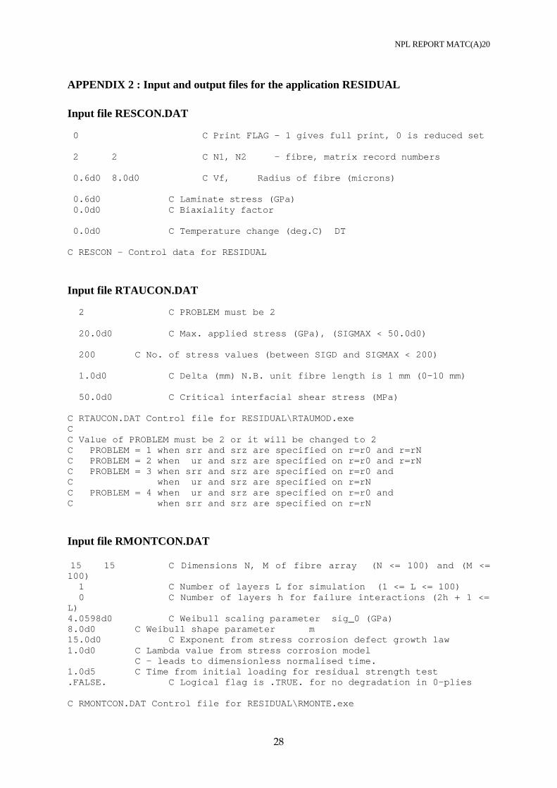
The data files given in Appendix 2 indicate the default control values that have been set for the RESIDUAL simulation. Their values are easily reset by editing the appropriate file in the RESIDUAL directory. Figs. 7-9 are easily constructed from the output data given in the files RMONPLT1.txt and RMONPLT2.txt. It should be noted that, in the interests of having relatively quick simulations only one layer has been included in the Monte Carlo model for the 0o plies. It should be noted that the results displayed in RMONPLT1.txt can be used to estimate the time to failure of the laminate when subject to a fixed applied load. This is achieved by setting the time before carrying out a residual strength test to a large number that ensures that the laminate has failed before the residual test can be executed. By setting this time to zero, the application RESIDUAL can be used to perform a static strength test.

Fig.7 : Dependence of the axial modulus ratio on the elapsed time since a fixed load was applied to the laminate.

0.980

0.985

0.990

0.995

1.000

0.0E+00 2.0E+05 4.0E+05 6.0E+05 8.0E+05 1.0E+06 1.2E+06

Normalised elapsed time

Axi

al m

od

ulu

s ra

tio


19

Fig.8 : Dependence of the axial strain% on the elapsed time since a fixed load was applied to the laminate.

Fig.9 : Dependence of the axial stress on the axial strain of the laminate during an

instantaneous residual strength test after the laminate has been subjected for a specified time to a fixed applied stress.

0.00

0.05

0.10

0.15

0.20

0.25

0.30

0.35

0.40

0.0 0.5 1.0 1.5 2.0 2.5 3.0

Axial strain %

Lam

inat

e ax

ial s

tres

s (G

Pa)

0.32

0.33

0.33

0.34

0.34

0.35

0.0E+00 2.0E+05 4.0E+05 6.0E+05 8.0E+05 1.0E+06 1.2E+06

Normalised elapsed time

Axi

al s

trai

n %


20

10.4 Conclusions regarding the RESIDUAL application

The application RESIDUAL enables predictions to be made of the time dependent degradation behaviour of cross-ply laminates arising from stress-corrosion mechanisms in the fibres of the 0o plies. By repeated execution of the application it is possible to generate stress-life curves, and also curves that show the time dependent degradation of the residual strength of the laminate. An example of one of these curves for a GRP is shown in Fig.10. The continuous line with diamond symbols shows the dependence of the normalised time to failure tf on the axial stress which is held fixed during the degradation process. The square symbols are predictions of the residual strength on the time t at which a fixed stress of 0.5 GPa has been applied to the laminate before the residual strength test was carried out. It should be noted that the residual strength results exhibit much more scatter than the lifetime predictions, and that the residual strength results are tending to the point on the lifetime curve corresponding to an axial stress of 0.5 GPa.

Fig. 10 : Example of typical results that can be generated using the application RESIDUAL.

The results for residual strength assume that a stress of 0.5 GPa was applied before the residual strength test is carried out.

11. Validation of models The key aspect of predictive modelling as far as design engineers are concerned is the reliability and robustness of the software that is used to predict the performance of composite laminates. When one examines the numerous materials parameters that are involved with the applications STRENGTH and RESIDUAL, the prospect of a thorough validation is virtually impossible on a short timescale. The approach taken here is to consider the validation of individual parts of the software by carrying out comparisons of model performance relative to other calculation methods (e.g. finite element analysis), and to experimental measurements. In Appendix 7 validation data (obtained through a collaboration with UMIST) are given that demonstrates that the concentric cylinder model on which fibre/matrix debonding is based,

0

0.2

0.4

0.6

0.8

1

1.2

0 2 4 6 8 10 12log10 tf or log10 t

Axi

al s

tres

s G

Pa

Time to failure

Residual strength


21

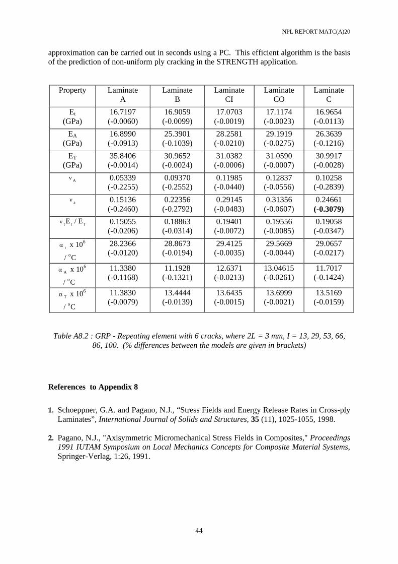
provides excellent estimates of the thermo-elastic properties of undamaged ply materials. This means that the applications STRENGTH and RESIDUAL can be used to predict the performance of cross-ply laminates from fibre/matrix properties. Appendix 8 presents the results from an informal collaboration with the Wright Laboratories, USAF, which has led to the confirmation that the NPL approximate method of dealing with the effects of non-uniform ply crack spacing, that arises during progressive ply crack formation, is exceedingly accurate. Furthermore, the collaboration has confirmed that the NPL model estimates of the thermo-elastic constants of a damaged cross-ply laminate are in very good agreement with values predicted by the more flexible (but less efficient) model developed at the Wright Laboratories. Appendix 9 shows comparisons of the predictions of the NPL ply cracking model with experimental data obtained at NPL for both GRP and CFRP laminates having various lay-ups. The results show that the model predictions agree very well with the measured values. Investigations have been undertaken where model predictions for the dependence of the axial modulus degradation on applied stress have been compared to experimental results. A key problem encountered concerns the determination of the stress-free temperature of the laminate, and whether its value varies with the thickness of the laminate. As predictions are tentative, they have not been included here. Further investigations will, however, be carried out in the MMS 4 project. Appendix 10 shows a comparison of the interfacial stress distributions predicted by the NPL stress-transfer model and those predicted by the boundary element system BEASY. The stress field is at the heart of procedures that must be followed when estimating the thermo-elastic properties of damaged laminates, and their accuracy is a key factor affecting model reliability and robustness. As the BEASY predictions may be regarded as an accurate estimate of the stress distributions, it is clear from the results presented in Appendix 10 that the NPL model is very accurate, and can be relied upon. While the ply cracking aspects of the modelling have been shown to be validated to a high quality, the validation of strength predictions and environmental degradation has only just begun. Initial attempts at validation have shown that model improvements are necessary, as already mentioned elsewhere in this report. Such model improvements and validation will continue in the MMS Projects 3 & 4.

12. Overall conclusions The applications STRENGTH and RESIDUAL described in this report must be regarded as the first steps towards the development of a predictive tool that will enable composite design engineers to develop damage resistant laminated materials, and to assess the strength and endurance performance of these materials. The STRENGTH application is an attempt to integrate software associated with various mechanism-based models into a computer system that can predict the strength of a laminate, taking account of biaxial loading and thermal residual stresses. The ply cracking module of the system is the most accurate developed to date that can operate on the timescales required by simulations that take minutes rather than hours/days to complete. The interface debonding module and Monte Carlo modules are likely to undergo further developments. The application RESIDUAL attempts to develop an integrated software system for composite laminates that takes some account of environmentally induced damage in the fibres.


22

It is concluded that, while a good start has been made developing a framework and preliminary models, much further development work is needed, as already mentioned in the report. This work relates to improvements in the models themselves (including extension to general symmetric laminates), continuation of model validation activities, and the development of a user-friendly design package that can easily be used by design engineers in the composites industry. These enhancements are planned in the forthcoming projects MMS3 and MMS4.

References 1. M J Hinton & P D Soden, ‘Predicting failure in composite laminates. The background to the

exercise’, Comp. Sci. Tech. 58, (1998), 1001-1010. 2. P D Soden, M J Hinton & A S Kaddour, ‘A comparison of the predictive capabilities of

current failure theories for composite laminates’, Comp. Sci. Tech. 58, (1998), 1225-1254. 3. L N McCartney, ‘Predicting non-linear behaviour in multiple-ply cross-ply laminates

resulting from micro-cracking’, in Proc. IUTAM Symposium on ‘Non-linear Analysis of Fracture’, Cambridge, 3-7 September 1995, Klewer Academic Publishers, Dordrecht-Boston-London, 1997, pp. 379-390.

4. L N McCartney, ‘Predicting transverse crack formation in cross-ply laminates resulting

from micro-cracking’, Comp. Sci & Tech. 58 (1998) 1069-1081. 5. L N McCartney, ‘Prediction of microcracking in composite materials’, in ‘FRACTURE: A

Topical Encyclopaedia of Current Knowledge Dedicated to Alan Arnold Griffith’, (ed. G.P.Cherepanov), Krieger Publishing Company, Melbourne, USA, to be published August 1998.

6. L.N.McCartney, ‘An effective stress controlling progressive damage formation in

laminates subject to triaxial loading’, Proc. Deformation & Fracture Conference, 18-19 March 1999, IoM Communications, London, pp. 23-32.

7. L.N.McCartney, ‘Simulation of progressive fibre failure during the tensile loading of

unidirectional composites’, NPL Report CMMT(A)212, August 1999. 8. L.N.McCartney, ‘Analytical model for debonded interfaces associated with fibre fractures

or matrix cracks’, in Proc. ICCM-12, Paris, July 1999. (A more detailed account has been written in paper from that is to be submitted for publication).

9. L.N.McCartney, ‘Model of composite degradation due to environmentally assisted fatigue

damage’, NPL Report MATC(A)26. 10.L.N.McCartney, ‘Model of composite degradation due to environmental damage’, NPL

Report CMMT(A)124, September 1998. 11.W Weibull, ‘A statistical distribution function of wide applicability’, J. Appl. Mech. 18,

(1951), 293-297.


23

12.B D Coleman, ‘On the strength of classical fibres and fibre bundles’, J Mech. Phys. Solids, 7, (1958), 60-70.

13.E J Gumbel, ‘Statistical theory of extreme values and some practical applications’, Nat. Bur.

Standards Appl. Maths. Series, 33, (1954).

Acknowledgement The report was prepared as part of the research undertaken for the Department of Trade and Industry funded project on CPD3, “Composites Performance and Design - Interface characterisation and behaviour”. It is also acknowledged that an earlier version of the Monte Carlo model presented in this report (neglecting effects of matrix and fibre/matrix debonding), and the carbon fibre Weibull distribution data, arose from participation in PREDICT. This project (Prediction of Damage Initiation and Growth in Composite Materials) was a collaboration between British Aerospace (Sowerby Research Centre), Ciba Geigy Plastics, Rolls Royce, Tenax Fibres, National Physical Laboratory, University of Bristol and the University of Surrey. The project was led by British Aerospace and was funded under the LINK Structural Composites programme of the DTI's Research and Technology Initiative (IED Grant Ref. RA 6/25/01).


24

APPENDIX 1 : Input and output files for the application STRENGTH Data file of fibre properties - FIBRE.dat 2 C (no. of fibres in file) 'AS4' 225.0 15.0 0.20 0.0714 15.0 -0.50d-6 1.50d-5 0.0 0.0 'Silenka ' 74.0 74.0 0.20 0.20 30.83333333 4.90d-6 4.90d-6 0.0 0.0 C TITLE EA ET NUA NUT MUA ALA ALT BEA BET

Data file of matrix properties - MATRIX.dat 2 C (no. of matrices in file) 'Epoxy35' 4.2 4.2 0.34 0.34 1.567164179 4.50d-5 4.50d-5 0.0 0.0 'EpoxyMY' 3.35 3.35 0.35 0.35 1.240740741 5.80d-5 5.80d-5 0.0 0.0 C TITLE EA ET NUA NUT MUA ALA ALT BEA BET

Input file STRGCON.DAT 0 C Print FLAG - 1 gives full print, 0 is reduced set 1 1 C Fibre and matrix record numbers (numbers depend user’s C input data file) 0.6d0 3.5d0 C Vf, Radius of fibre (microns) 0.2d0 C Biaxiality factor -157.0d0 C Temperature change (deg.C) DT C STRGCON - Control data for STRENGTH Input file STAUCON.DAT 2 C PROBLEM (Must use value 2) 10.0d0 C Max. value of applied stress (GPa), (SIGMAX < 50.0d0) 200 C No. of stress values between SIGD and SIGMAX ( < 200) 1.0d0 C Value of delta (mm) N.B. unit fibre length is 1 mm (0-10 mm) 50.0d0 C Value of the critical interfacial shear stress (MPa) C STAUCON.DAT Control file for STRENGTH\STAUMOD.exe C C Value of PROBLEM (1..4) C PROBLEM = 1 when srr and srz are specified on r=r0 and r=rN C PROBLEM = 2 when ur and srz are specified on r=r0 and r=rN C PROBLEM = 3 when srr and srz are specified on r=r0 and C when ur and srz are specified on r=rN C PROBLEM = 4 when ur and srz are specified on r=r0 and C when srr and srz are specified on r=rN


25

Input file SMONTCON.DAT 15 15 C Dimensions N, M of fibre array (N <= 50) and (M <= 50) 1 C Number of layers L for simulation (1 <= L <= 100) 5.801d0 C Weibull scaling parameter sig_0 (GPa) 8.0d0 C Weibull shape parameter m C SMONTCON.DAT; Control file for STRENGTH\SMONTE.exe C C For 1 mm lengths of fibre : C Weibull scaling parameter sig_0 (GPa) C Weibull shape parameter m Input file SXMODCON.DAT 25.0d0 C LAMLENGTH (mm) 200 C No. of cracking sites (MAX 1024) 2 C No. of plies (not elements) - up to 16 1 1 0.26d0 5 2 C Angle, Damage, Thickness, Elems, Divs 0 0 0.26d0 5 2 C SXMODCON; Control data for STRENGTH\SXMOD to generate data for SXRAND C C FOR each ply :- C C Angle ( = 0 for 0 deg, = 1 for 90 deg) C Damage (0 = no, 1 = yes) Thickness (mm) C No. of basic elements (>0) No. of sub-divisions at interface

Input file SXRNDCON.DAT 110.0d0 C Mean Energy gamma (NOT 2xgamma) 15.0d0 C Standard deviation alpha% 5.0d0 C RHO (max. crack density) C SXRNDCON - Control data for STRENGTH\SXRAND C C RHO will be reset if necessary when RHOMAX is known The following output files are produced by the above input files for the STRENGTH application, and are provided here so that users can check that their software installation is working correctly, and to provide a record of software performance for quality purposes. The files shown are the only ones created when the Print Flag is set to zero. Many more output files are generated when the flag is set to unity.


26

Output file STRGOUT.TXT STRENGTH Version 1.0 - 30/03/2000 Run on 02/06/2001 at 13:08:12 Using fibre properties for AS4; matrix properties for Epoxy35 0 hexagonal fibre rings Values of elastic constants for different phases Phase Number 1 2 UD Composite EA: Axial Youngs mod. GPa 225.00000 4.20000 136.70323 ET: Trans.Youngs mod. GPa 15.00000 4.20000 8.92997 NA: Axial Poisson s ratio 0.20000 0.34000 0.25264 NT: Trans.Poisson s ratio 0.07140 0.34000 0.30589 KT: Trans.bulk mod. GPa 8.12333 4.89739 6.51089 MUA: Axial shear mod. GPa 15.00000 1.56716 4.53653 MUT: Trans.shear mod. GPa 7.00019 1.56716 3.41911 ALA: Axial T E coeff. x1E6 -0.50000 45.00000 0.11437 ALT: Trans.T E coeff. x1E6 15.00000 45.00000 31.94012 r micro.m 3.50000 4.51848 4.51848 Volume fraction (phase 1) = 0.600000000 Biaxiality factor for Transverse Stress = 0.200 Temperature change during manufacture = -157.000 deg C ================================== SXMOD input data Fibre is AS4 Matrix is Epoxy35 2 plies. For each ply: Angle Damage ThicknessNo. elemen No. sub-divs 1 1 0.2600 5 2 0 0 0.2600 5 2 Total laminate thickness = 1.0400 mm Initial crack density fixed 200 Cracking Sites to be generated; Laminate length = 25.0000 mm Properties for the undamaged Laminate EA ET NUA ALA ALT 7.3051D+01 7.3051D+01 3.0982D-02 2.4854D-06 2.4854D-06 First pass SXMOD ends successfully ================================== STAUMOD PROBLEM = 2 Lambda = 0.000 FIBRE FRACTURE Temperature Change = -157.000 C; Delta = 1.000 mm STAUMOD ends successfully ================================== Effective modulus before first fibre failure (GPa) = 138.623681622 Failure Strain% Laminate Stress (GPa) Modulus ratio of 0-plies before next fibre break 1.359726D+00 1.028174D+00 1.000000D+00 1.513491D+00 1.137983D+00 9.964215D-01 1.563911D+00 1.172013D+00 9.936936D-01 1.581427D+00 1.182265D+00 9.914453D-01 1.585903D+00 1.183249D+00 9.894850D-01 1.592365D+00 1.185592D+00 9.874582D-01 1.686909D+00 1.239024D+00 9.749062D-01 1.710258D+00 1.252099D+00 9.719252D-01 1.734869D+00 1.265785D+00 9.687952D-01


27

1.743992D+00 1.269445D+00 9.665621D-01 1.748228D+00 1.269997D+00 9.646472D-01 1.755349D+00 1.271502D+00 9.618911D-01 1.772345D+00 1.279861D+00 9.590394D-01 First pass SMONTE ends successfully ================================== Laminate stress > laminate failure stress. First pass SXRAND ends successfully Properties for the undamaged Laminate EA ET NUA ALA ALT 7.2807D+01 7.3051D+01 3.0983D-02 2.4934D-06 2.4852D-06 7.2620D+01 7.3051D+01 3.0983D-02 2.4995D-06 2.4850D-06 7.2467D+01 7.3051D+01 3.0983D-02 2.5046D-06 2.4849D-06 7.2333D+01 7.3051D+01 3.0983D-02 2.5090D-06 2.4848D-06 7.2194D+01 7.3051D+01 3.0983D-02 2.5136D-06 2.4846D-06 7.1336D+01 7.3050D+01 3.0984D-02 2.5425D-06 2.4838D-06 Laminate stress > laminate failure stress. Second pass SXRAND ends successfully ==================================

Output file XRNDPLT1.TXT (main results with no fibre failures) EPS'%, SIG (GPa), RHO (/mm), EAC (GPa), NUAC, ALAC*1E6 (/deg C), 0.000000, 0.000000, 0.000000, 73.0513, 0.030982, 2.4854, 0.229639, 0.168800, 0.000000, 73.0513, 0.030982, 2.4854, 0.230663, 0.168800, 0.040000, 72.9443, 0.030610, 2.4428, 0.239043, 0.174951, 0.040000, 72.9443, 0.030610, 2.4428, 0.240079, 0.174951, 0.080000, 72.8376, 0.030238, 2.4001, 0.262015, 0.191026, 0.080000, 72.8376, 0.030238, 2.4001, 0.263086, 0.191026, 0.120000, 72.7313, 0.029868, 2.3575, ....... 1.792731, 1.232469, 2.440000, 69.4207, 0.018340, 0.9644, 1.793255, 1.232469, 2.480000, 69.4051, 0.018285, 0.9575, 1.793998, 1.232986, 2.480000, 69.4051, 0.018285, 0.9575, 1.794523, 1.232986, 2.520000, 69.3895, 0.018231, 0.9507, 1.808283, 1.242570, 2.520000, 69.3895, 0.018231, 0.9507, 1.808811, 1.242570, 2.560000, 69.3740, 0.018177, 0.9438, 1.841326, 1.265209, 2.560000, 69.3740, 0.018177, 0.9438, 1.841861, 1.265209, 2.600000, 69.3584, 0.018123, 0.9369,

Output file XRNDPLT2.TXT (main results with fibre failures) EPS'%, SIG (GPa), RHO (/mm), EAC (GPa), NUAC, ALAC*1E6 (/deg C), 0.000000, 0.000000, 0.000000, 73.0513, 0.030982, 2.4854, 0.229639, 0.168800, 0.000000, 73.0513, 0.030982, 2.4854, 0.230663, 0.168800, 0.040000, 72.9443, 0.030610, 2.4428, 0.239043, 0.174951, 0.040000, 72.9443, 0.030610, 2.4428, 0.240079, 0.174951, 0.080000, 72.8376, 0.030238, 2.4001, 0.262015, 0.191026, 0.080000, 72.8376, 0.030238, 2.4001, 0.263086, 0.191026, 0.120000, 72.7313, 0.029868, 2.3575, 0.280940, 0.204089, 0.120000, 72.7313, 0.029868, 2.3575, ...... 1.796801, 1.203657, 2.520000, 67.6736, 0.018230, 0.9716, 1.810570, 1.213009, 2.520000, 67.6736, 0.018230, 0.9716, 1.811110, 1.213009, 2.560000, 67.6580, 0.018176, 0.9645, 1.843647, 1.235103, 2.560000, 67.6580, 0.018176, 0.9645, 1.844195, 1.235103, 2.600000, 67.6425, 0.018122, 0.9575,


28

APPENDIX 2 : Input and output files for the application RESIDUAL Input file RESCON.DAT 0 C Print FLAG - 1 gives full print, 0 is reduced set 2 2 C N1, N2 - fibre, matrix record numbers 0.6d0 8.0d0 C Vf, Radius of fibre (microns) 0.6d0 C Laminate stress (GPa) 0.0d0 C Biaxiality factor 0.0d0 C Temperature change (deg.C) DT C RESCON - Control data for RESIDUAL Input file RTAUCON.DAT 2 C PROBLEM must be 2 20.0d0 C Max. applied stress (GPa), (SIGMAX < 50.0d0) 200 C No. of stress values (between SIGD and SIGMAX < 200) 1.0d0 C Delta (mm) N.B. unit fibre length is 1 mm (0-10 mm) 50.0d0 C Critical interfacial shear stress (MPa) C RTAUCON.DAT Control file for RESIDUAL\RTAUMOD.exe C C Value of PROBLEM must be 2 or it will be changed to 2 C PROBLEM = 1 when srr and srz are specified on r=r0 and r=rN C PROBLEM = 2 when ur and srz are specified on r=r0 and r=rN C PROBLEM = 3 when srr and srz are specified on r=r0 and C when ur and srz are specified on r=rN C PROBLEM = 4 when ur and srz are specified on r=r0 and C when srr and srz are specified on r=rN

Input file RMONTCON.DAT 15 15 C Dimensions N, M of fibre array (N <= 100) and (M <= 100) 1 C Number of layers L for simulation (1 <= L <= 100) 0 C Number of layers h for failure interactions (2h + 1 <= L) 4.0598d0 C Weibull scaling parameter sig_0 (GPa) 8.0d0 C Weibull shape parameter m 15.0d0 C Exponent from stress corrosion defect growth law 1.0d0 C Lambda value from stress corrosion model C - leads to dimensionless normalised time. 1.0d5 C Time from initial loading for residual strength test .FALSE. C Logical flag is .TRUE. for no degradation in 0-plies C RMONTCON.DAT Control file for RESIDUAL\RMONTE.exe


29

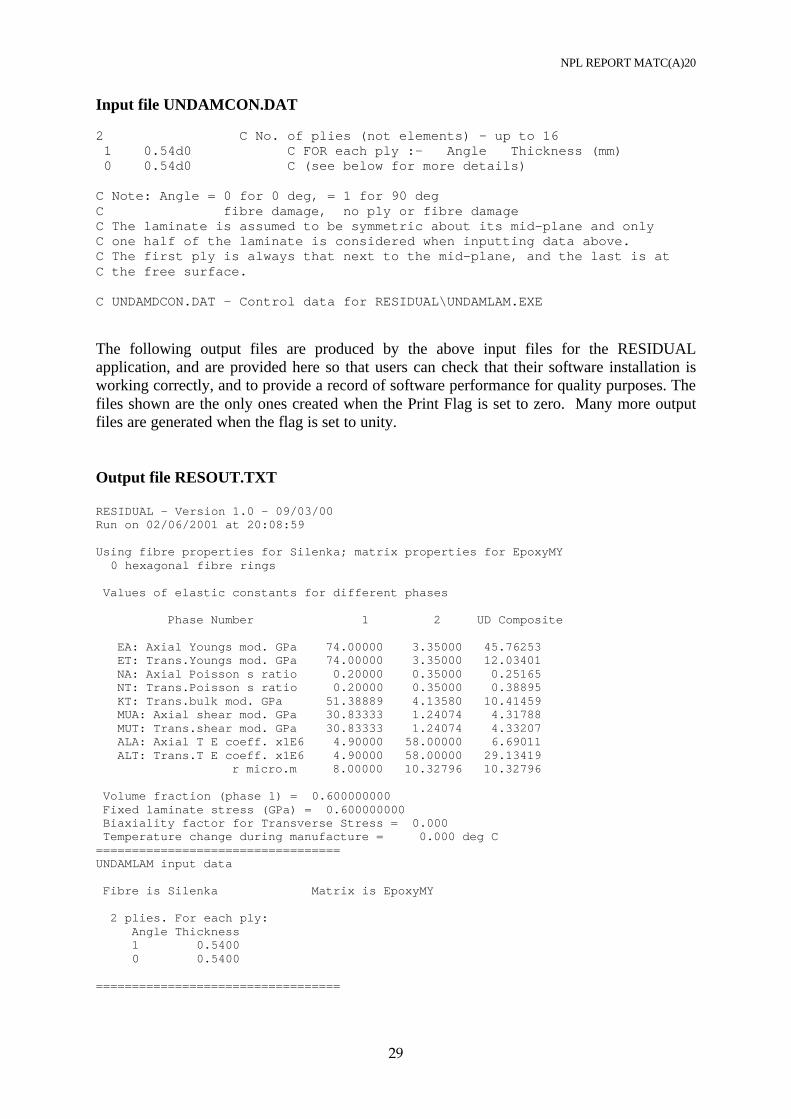
Input file UNDAMCON.DAT 2 C No. of plies (not elements) - up to 16 1 0.54d0 C FOR each ply :- Angle Thickness (mm) 0 0.54d0 C (see below for more details) C Note: Angle = 0 for 0 deg, = 1 for 90 deg C fibre damage, no ply or fibre damage C The laminate is assumed to be symmetric about its mid-plane and only C one half of the laminate is considered when inputting data above. C The first ply is always that next to the mid-plane, and the last is at C the free surface. C UNDAMDCON.DAT - Control data for RESIDUAL\UNDAMLAM.EXE

The following output files are produced by the above input files for the RESIDUAL application, and are provided here so that users can check that their software installation is working correctly, and to provide a record of software performance for quality purposes. The files shown are the only ones created when the Print Flag is set to zero. Many more output files are generated when the flag is set to unity. Output file RESOUT.TXT RESIDUAL - Version 1.0 - 09/03/00 Run on 02/06/2001 at 20:08:59 Using fibre properties for Silenka; matrix properties for EpoxyMY 0 hexagonal fibre rings Values of elastic constants for different phases Phase Number 1 2 UD Composite EA: Axial Youngs mod. GPa 74.00000 3.35000 45.76253 ET: Trans.Youngs mod. GPa 74.00000 3.35000 12.03401 NA: Axial Poisson s ratio 0.20000 0.35000 0.25165 NT: Trans.Poisson s ratio 0.20000 0.35000 0.38895 KT: Trans.bulk mod. GPa 51.38889 4.13580 10.41459 MUA: Axial shear mod. GPa 30.83333 1.24074 4.31788 MUT: Trans.shear mod. GPa 30.83333 1.24074 4.33207 ALA: Axial T E coeff. x1E6 4.90000 58.00000 6.69011 ALT: Trans.T E coeff. x1E6 4.90000 58.00000 29.13419 r micro.m 8.00000 10.32796 10.32796 Volume fraction (phase 1) = 0.600000000 Fixed laminate stress (GPa) = 0.600000000 Biaxiality factor for Transverse Stress = 0.000 Temperature change during manufacture = 0.000 deg C ================================== UNDAMLAM input data Fibre is Silenka Matrix is EpoxyMY 2 plies. For each ply: Angle Thickness 1 0.5400 0 0.5400 ==================================


30

RTAUMOD PROBLEM = 2 Lambda = 0.000 FIBRE FRACTURE Temperature Change = 0.000 C; Delta = 1.000 mm RTAUMOD ends successfully ================================== Effective modulus before first fibre failure (GPa) = 46.2148011788 Failure Strain% Laminate Stress (GPa) Modulus ratio Normalised time of 0-plies before next fibre break 2.067463D+00 6.000000D-01 9.984907D-01 -1.562600D+02 2.073058D+00 6.000000D-01 9.969803D-01 6.495659D+02 2.078680D+00 6.000000D-01 9.954689D-01 1.029160D+04 2.084329D+00 6.000000D-01 9.939564D-01 2.167577D+04 2.090005D+00 6.000000D-01 9.924428D-01 4.511744D+04 2.095708D+00 6.000000D-01 9.909282D-01 6.808160D+04 2.101439D+00 6.000000D-01 9.894125D-01 6.929578D+04 2.107197D+00 6.000000D-01 9.878957D-01 7.304214D+04 2.112983D+00 6.000000D-01 9.863779D-01 1.037593D+05 Failure Strain% Laminate Stress (GPa) Modulus ratio of 0-plies before next fibre break 2.112983D+00 6.000000D-01 9.863779D-01 3.233112D+00 8.954660D-01 9.632538D-01 3.345182D+00 9.056287D-01 9.591970D-01 3.401341D+00 9.152591D-01 9.565369D-01 3.460205D+00 9.263330D-01 9.537041D-01 3.491109D+00 9.285193D-01 9.496853D-01 3.698865D+00 9.730772D-01 9.424517D-01 3.753299D+00 9.734536D-01 9.346840D-01 3.900971D+00 9.909097D-01 9.213281D-01 3.990176D+00 9.968524D-01 9.162873D-01 4.124044D+00 9.979363D-01 8.912782D-01 RMONTE ends successfully ==================================

Output file RMONPLT1.TXT (Response when stress is held fixed prior to residual strength test) ' Failure Strain% Laminate Stress (GPa) Modulus ratio Normalised time' ' of 0-plies before next fibre break' 2.067463E+00, 6.000000E-01, 9.984907E-01, -1.562600E+02, 2.073058E+00, 6.000000E-01, 9.969803E-01, 6.495659E+02, 2.078680E+00, 6.000000E-01, 9.954689E-01, 1.029160E+04, 2.084329E+00, 6.000000E-01, 9.939564E-01, 2.167577E+04, 2.090005E+00, 6.000000E-01, 9.924428E-01, 4.511744E+04, 2.095708E+00, 6.000000E-01, 9.909282E-01, 6.808160E+04, 2.101439E+00, 6.000000E-01, 9.894125E-01, 6.929578E+04, 2.107197E+00, 6.000000E-01, 9.878957E-01, 7.304214E+04, 2.112983E+00, 6.000000E-01, 9.863779E-01, 1.037593E+05,


31

Output file RMONPLT2.TXT (Response when stress during the residual strength test) ' Failure Strain% Laminate Stress (GPa) Modulus ratio' ' of 0-plies before next fibre break' 2.112983E+00, 6.000000E-01, 9.863779E-01, 3.233112E+00, 8.954660E-01, 9.632538E-01, 3.345182E+00, 9.056287E-01, 9.591970E-01, 3.401341E+00, 9.152591E-01, 9.565369E-01, 3.460205E+00, 9.263330E-01, 9.537041E-01, 3.491109E+00, 9.285193E-01, 9.496853E-01, 3.698865E+00, 9.730772E-01, 9.424517E-01, 3.753299E+00, 9.734536E-01, 9.346840E-01, 3.900971E+00, 9.909097E-01, 9.213281E-01, 3.990176E+00, 9.968524E-01, 9.162873E-01, 4.124044E+00, 9.979363E-01, 8.912782E-01,


32

APPENDIX 3 : Calculation procedure for STRENGTH application 1. Read in fibre and matrix properties from a purpose built data base. 2. Use a concentric cylinder model to estimate (and print out) all the effective thermo-elastic

constants of an undamaged unidirectional composite having the same fibre volume fraction as the plies of the cross-ply laminate.

11. Estimate and store the values of all the non-shear thermoelastic constants for the cross-ply

laminate in an undamaged state. 12. Use the application TAUMOD to create a look-up table that describes the tensile

mechanical behaviour of a fibre/matrix cell following fibre fracture, taking account of the state of biaxial loading, thermal residual stresses, and of fibre/matrix debonding (or shear yielding) that is characterised by a uniform interfacial shear stress τ .

13. Allocate fibre strengths at random (using a Weibull distribution) to all the fibre/matrix cells

included in the simulation. 14. Use the application MONTE to predict the axial stress values at which successive fibre

breaks occur in the 0o plies of the laminate up to the point of instability where the composite breaks into two distinct pieces. For each stress value at which a fibre breaks, the effective axial modulus is also estimated. The ratios, defined by dividing these effective moduli values by the undamaged modulus predicted by TAUMOD, are estimated and stored for use when predicting ply crack formation.

15. Use the application PREDICT to simulate ply crack formation without taking account of

the effects of fibre fracture. 16. Repeat the procedure to simulate ply crack formation taking account of the effects of fibre

fracture up to the point of catastrophic failure of the laminate that is assumed to occur when the effective stress in the 0o plies is equal to the failure stress predicted by MONTE. The fracture energies used to predict ply crack formation are distributed on the potential crack formation sites in an identical way to that used when carrying out Stage 7. The comparison of the results of these simulations enables a determination of the effect of fibre fracture during the simulation.


33

APPENDIX 4 : Monte Carlo simulation procedure for STRENGTH and RESIDUAL 1. Set the failure flags to ‘true’, signifying that all fibre elements in the fibre/matrix cells are

intact. 2. Using the failure strengths allocated to each fibre element, calculate the corresponding

failure strains of the fibre elements in each cell. 3. Scan all fibre/matrix cells in the system to determine the fibre element in the system that

has the lowest failure strain. 4. Apply loading until the fibre element with least strength is just about to fail. 5. Allow the fibre element to fail and set the flag of the failed fibre element to ‘false’. 6. Assess whether composite has failed using criterion described in section 6. 7. Redistribute the load carried by the fibre/matrix cell containing the fibre element that has

just failed using prescribed load-sharing methodology described in [7]. Update the strain values for all fibre/matrix cells, and the effective modulus of the damaged cells.

8. Scan all fibre matrix cells to determine the fibre element (if any) that has exceeded its

failure strain by the greatest amount. If such a fibre element is found then go to stage 4 and repeat as before. If no such fibre elements are found then the state of the system, following a fibre element failure and resultant stress redistribution, has led to a stable configuration where mechanical equilibrium can be maintained.

9. Scan all fibre/matrix cells to determine the fibre element that is closest to its failure strain

and then increase the applied load so that this fibre element is just about to fail, checking that each layer is supporting the same load.

10. Calculate the mean strain and the corresponding effective axial modulus for the composite.

Go to Stage 4. 11. Stop the simulation when it is clear that no further stable equilibrium states will be

predicted.


34

APPENDIX 5 : Operation of the STRENGTH application A description will now be given regarding the operation of the application STRENGTH that estimates the effects of damage on cross-ply laminates up to the point of failure. The software is run in two stages. For the first stage, ply cracking is the only form of damage that is allowed. This is quickly carried out before the second stage is initiated which repeats the simulation but allows fibre fracture and interface debonding to occur enabling estimates to be made of the failure strain and the strength. It is emphasised that the results of the simulation are based on a statistical model of fibre failure with the result that the output of the application will change every time the software is run. It is thus not possible to provide a standard solution that can be used to check that the software is operating correctly. Such standard solutions are possible, however, when fibre fracture is ignored. When running the executable file strength.exe the following sequence of events is followed:

N.B. It is recommended that this list is read only when using the application for the first time. A Help drop down menu appears in each window.

1. The title screen first appears giving the user the choice of selecting ‘continue’, ‘default’

and ‘stop’ buttons. The ‘stop’ button terminates the application immediately. The button ‘default’ uses a list of pre-determined settings that minimise user interaction with the application. The ‘continue’ button enables the user to see the default values that are already set and to change them as appropriate. The default values are stored in the following files : strgcon.dat, smontcon.dat, staucon.dat, sxmodcon.dat and sxrndcon.dat. The default files can only be changed by editing these files. The next version of STRENGTH will be modified so that default files can be altered during the data selection procedure part of a simulation. If the default option is selected then the application operates automatically to the point where the simulation has been completed for the first case where fibre damage is NOT allowed. The results at this stage of the simulation can be used for validation of the ply cracking part of the model, and the user can check that his installed version of the software is working correctly (see Appendix 1).

2. If the ‘continue’ button has been selected then the user is asked to check or change all the

input data for the simulation by interaction with the screen using the mouse. For each screen that appears, there is a help menu that gives brief details regarding the nature of the input parameters that appear in the window.

3. The first screen that appears is concerned with the selection of fibre and matrix materials.

Two boxes appear showing the choices of material that can be used. The selection is made by clicking on the material for both fibre and matrix, and then clicking the ‘select’ button.

4. The next window that appears concerns the print flag. When set to zero the minimum

amount of information is printed. This would be used during production runs of the application. When set to unity, more information is printed out enabling the user to investigate in more detail the operation of the application. This option would normally be used only by program developers when trouble-shooting.


35

5. The next window inputs the fibre volume fraction, the fibre radius and the temperature change during manufacture, i.e. an estimate of the stress-free temperature of the composite that is used for both fibre/matrix and laminate models.

6. The next window inputs the biaxiality factor K that determines the transverse stress

applied to the laminate, namely, Kσ , where σ is the axial stress applied to the laminate. 7. The next executable file for the prediction of ply cracking can now be used by clicking on

the ‘continue’ button. The number of plies in the laminate is then entered followed by the input of information that defines the orientation, damage state, thickness, and ply refinement that are to be used in the simulation. The item labelled ‘number of elements’ defines the number of elements (i.e. sub-plies) into which the ply is to be sub-divided, and the number of sub-divisions specifies the number of times the element at an interface is successively split into two equal elements. This sub-division of elements would be carried out only at those interfaces where a ply crack tip will be located. This ply refinement procedure is essential if accurate stress distributions are to be obtained. It is usual to choose a value of 2 or 3. Selecting a larger value can result in plies being too thin and subsequent software failure because of numerical instabilities.

8. The next window inputs the length of laminate that is considered by the simulation. This

is selected to be large enough to be representative of the complete laminate, but should be at least 25 mm. Increasing this length will require an increase in the number of ply cracks to be generated, thus leading to increased execution times.

9. The next window inputs the number of potential sites in the length of laminate simulated

at which ply cracks might form during loading. This should be at least 100 and larger values will again lead to longer execution times.

10. The next window concerns the Monte Carlo modelling of fibre failure in the 0o plies of

the laminate. The value of ‘Problem type’ to input should always be 2, a selection that imposes conditions on the external surface of the representative fibre/matrix cell that would be relevant for a fibre embedded in a composite. Such conditions apply a zero shear stress and a uniform interfacial displacement normal to the external surface that corresponds to that found in an undamaged unidirectional composite subject to the same axial and transverse stresses, and temperature.

11. The next window is concerned with the generation of a look-up table that models the

stress-strain behaviour of the fibre/matrix cell when the fibre has failed. A maximum axial stress applied to the cell is specified which is usually at least 5 GPa. The large value of the axial stress is necessary to cater for stress transfer during the latter stages of the simulation where the composite progressively fails without stabilising at an equilibrium state. If, for example, the simulation was run until the last fibre had failed then the stress on the last surviving fibre/matrix cell would be exceedingly large. The interfacial shear stress is also input in this window, representing the shear stress that is assumed to act at the fibre/matrix interface in the debonded region of the fibre (except for a small transition zone on the interface near the fibre fracture).


36

12. The next window inputs the length of the fibre/matrix cells used in the Monte Carlo simulation. The fibre strengths are allocated to the cells using the Weibull strength distribution, taking proper account of their length. If this length is selected to be too small then it will require many layers of elements to represent a reasonable length of the laminate and this will result in considerable execution times.

13. The next window inputs the number of values in the look-up table representing the

mechanical behaviour of the fibre/matrix cells following fibre fracture. The number required is the number of stress increments between the debonding stress and the maximum stress that is applied. At least 100 stress increments are normally used. This data value would be best input at the same time as the maximum stress (see Item 11). This modification will be implemented in the next version of the software.

14. The dimensions of the fibre array are the next values to be inputted. The parameters N

and M define a hexagonal array of 2MN fibres on a rectangular lattice. Usually M = N and the largest suggested value is 30, leading to long execution times.

15. The number L of layers used in the Monte Carlo simulation is next input. Its selection is

made in conjunction with the element length (see Item 12). Too large a value will again lead to very long execution times. (The next version of the software will input this parameter following the selection of the element length (Item 12) )

16. The Weibull parameters m and σo are the next parameters to be specified (see Section

8.3 for more details). 17. The application then automatically calls the random ply cracking executable that first

requires the input of the mean fracture energy for ply cracking (note that the value g is needed, and not 2γ which is the parameter corresponding to the long crack limit of the critical energy release rate for ply cracking), the standard deviation of the fracture energy distribution expressed as a percentage of the mean fracture energy, and the maximum crack density to be used during the first stage of the simulation where fibre fracture does not occur.

18. The first stage of the simulation is then executed and the user is given the opportunity of

examining and printing various plots that can be constructed from the results window. The results of this stage can be used by the user for validation purposes, and to check that the software is working correctly (see Appendix 1). On selecting ‘exit’ from this window the application then repeats the simulation to the point of failure for the case where fibre fracture and interface debonding is allowed to occur. On completion of the simulation the user again is given the opportunity of examining plots of results and of printing the graphs.

19. The numerical data given in the graphs for both stages of the simulation can be found in

the files XRNDPLT1.txt (no fibre failure) and XRNDPLT2.txt (with fibre failures). Other output files may be found in the files: STRGOUT.txt, STAUOUT.txt, SMONTOUT.txt, SXMODOUT.txt and SRNDOUT.txt.


37

APPENDIX 6 : Operation of the RESIDUAL application A description will now be given of the application RESIDUAL that is designed to predict the degradation of a cross-ply laminate subject to environmental exposure. For this case, the only damage modes that are considered are the time dependent failure of the fibres in the 0o plies resulting from environmentally driven defect growth, and the associated interfacial failure between fibre and matrix. The simulation does not allow ply crack formation, and it is assumed that the degradation of the 90o plies is ignored as it is not expected to contribute significantly to the degradation of the laminate. The application can be used to predict an estimate of the lifetime of the laminate and the time dependence of the residual strength. It is emphasised again that the results of the simulation are based on a statistical model of fibre failure with the result that the output of the application will change every time the software is run. It is thus not possible to provide a standard solution that can be used to check that the software is operating correctly. When running the executable file strength.exe the following sequence of events are followed:

N.B. It is recommended that this list is read only when using the application for the first time. A Help drop down menu appears in each window.

1. The title screen first appears giving the user the choice of selecting ‘continue’, ‘default’

and ‘stop’ buttons. The ‘stop’ button terminates the application immediately. The button ‘default’ uses a list of pre-determined settings that minimise user interaction with the application. The ‘continue’ button enables the user to see the default values that are already set and to change them as appropriate. The default values are stored in the following files : rescon.dat, rmontcon.dat, rtaucon.dat and undamcon.dat. The default files can only be changed by editing these files. The next version of RESIDUAL will be modified so that default files can be altered during the data selection procedure part of a simulations. If the default option is selected then the application operates automatically to the end of the simulation.

2. If the ‘continue’ button has been selected then the user is asked to check or change all the

input data for the simulation by interaction with the screen using the mouse. For each screen that appears, there is a help menu that gives brief details regarding the nature of the input parameters that appear in the window.

3. The first screen that appears is concerned with the selection of fibre and matrix materials.

Two windows appear showing the choices of material that can be used. The selection is made by clicking on the material for both fibre and matrix, and then clicking the ‘select’ button.

4. The next window that appears concerns the print flag. When set to zero the minimum

amount of information is printed. This would be used during production runs of the application. When set to unity, more information is printed out enabling the user to investigate in more detail the operation of the application. This option would normally be used only by program developers when trouble-shooting.


38

5. The next window inputs the fibre volume fraction, the fibre radius and the temperature change during manufacture, i.e. an estimate of the stress-free temperature of the composite which is used for both fibre/matrix and laminate models.

6. The next window inputs the value of the axial stress σ that is applied to the laminate and

then held fixed, and the value of the biaxiality factor K which determines the transverse stress applied to the laminate, namely, Kσ .

7. The next executable file for the prediction of lifetime and residual strength can now be

used by clicking on the ‘continue’ button. The first window to open requires the number of plies in the laminate that are to be used in the simulation and the following window asks to user to specify the orientation of each ply. It is assumed that all 0o plies are subject to fibre damage, and that the 90o plies remain undamaged. (Note: As ply cracking is not being considered the way in which the 90o and 0o plies are arranged in the laminate does not make a difference to predictions). The user can then either inspect the output file undamout.txt or select exit to continue the simulation.

8. The next window concerns the Monte Carlo modelling of fibre failure in the 90o plies of

the laminate. The value of ‘Problem type’ to input should always be 2, a selection that imposes conditions on the external surface of the representative fibre/matrix cell that would be relevant for a fibre embedded in a composite. Such conditions apply a zero shear stress and a uniform interfacial displacement normal to the external surface that corresponds to that found in an undamaged unidirectional composite subject to the same axial and transverse stresses, and temperature.

9. The next window is concerned with the generation of a look-up table that models the

stress-strain behaviour of the fibre/matrix cell when the fibre has failed. A maximum axial stress applied to the cell is specified which is usually at least 5 GPa. The large value of the axial stress is necessary to cater for stress transfer during the latter stages of the simulation where the composite progressively fails without stabilising at an equilibrium state. If, for example, the simulation was run until the last fibre had failed then the stress on the last surviving fibre/matrix cell would be exceedingly large. The interfacial shear stress is also input in this window, representing the shear stress that is assumed to act at the fibre/matrix interface in the debonded region of the fibre (except for a small transition zone on the interface near the fibre fracture).

10. The next window inputs the length of the fibre/matrix cells used in the Monte Carlo

simulation. The fibre strengths are allocated to the cells using the Weibull strength distribution and taking proper account of their length. If this length is selected to be too small then it will require many layers of elements to represent a reasonable length of the laminate and this will result in considerable execution times.

11. The next window inputs the number of values in the look-up table representing the

mechanical behaviour of the fibre/matrix cells following fibre fracture. The number required is the number of stress increments between the debonding stress and the maximum stress that is applied. At least 100 stress increments are normally used. This data value would be best input at the same time as the maximum stress (see Item 9). This modification will be implemented in the next version of the software.


39

12. The dimensions of the fibre array are the next values to be inputted. The parameters N and M define a hexagonal array of 2MN fibres on a rectangular lattice. Usually M = N and the largest suggested value is 30, leading to long execution times.

13. The number L of layers used in the Monte Carlo simulation is next input. Its selection is

made in conjunction with the element length (see Item 10). Too large a value will again lead to very long execution times. (The next version of the software will input this parameter following the selection of the element length).

14. The Weibull parameters m and σo are the next parameters to be specified (see Section

8.3 for more details). 15. The next window concerns the input of parameters needed to operate the fibre failure

mechanism. The first value is the exponent n in the fibre defect growth law (5). The second is the parameter L needed by the stress-corrosion model of fibre failure. This value can be set to unity in which case the normalised times used by the simulation are dimensionless and are defined in a particular way (see Section 8.6). The third value required is the dimensionless ‘time’ for which the fixed loads σ σ, K are applied before a residual strength ‘test’ is carried out by the simulation.

16. On completion of the simulation the user is given the opportunity of examining plots of

results and of printing the graphs. 17. The numerical data given in the graphs for both stages of the simulation can be found in

the files RMONPLT1.txt and RMONPLT2.txt. Other output data may be found in the files RESOUT.txt, RTAUOUT.txt and RMONTOUT.txt.


40

APPENDIX 7 : Validation data for software used to predict undamaged ply properties from fibre and matrix data Through a collaboration with Dr Shuguang Li (Dept. Mechanical Engineering, UMIST) the validation data presented in Tables A7.1-4 has been compiled for a CFRP and GRP used in the International Failure Exercise. The Li & Zou data have been obtained by FEA and are expected to be the best estimates of the thermoelastic constants of undamaged ply material, and they are the yardstick against which the software routines are being assessed. Predictions made using the NPL developed software system CoDA (Composites Design & Analysis) are also included in the Tables.

Fibre and matrix data for CFRP (AS4 carbon fibre and epoxy)

Matrix Young's modulus 4.2 (GPa) Matrix Poisson's ratio 0.34 Fibre longitudinal Young's modulus 225 (GPa) Fibre transverse Young's modulus 15 (GPa) Fibre longitudinal Poisson's ratio 0.2 Fibre longitudinal shear modulus 15.0 (GPa) Fibre transverse shear modulus 7 (GPa) Matrix thermal expansion coefficient 45 (10-6/°C) Fibre longitudinal thermal expansion coefficient -0.5 (10-6/°C) Fibre transverse thermal expansion coefficient 15 (10-6/°C) Fibre volume fraction 60 %

Table A7.1 : Properties of AS4 fibre and epoxy matrix.

Lamina properties Exercise

(Expt.) Li & Zou NPL model CoDA

Longitudinal Young's modulus EA

126 (GPa) 136.70 (GPa) 136.70 (GPa) 136.68 (GPa)

Transverse Young's modulus ET

11 (GPa) 8.901 (GPa) 8.930 (GPa) 9.026 (GPa)

Longitudinal shear modulus µA

6.6 (GPa) 4.550 (GPa) 4.536 (GPa) 4.537 (GPa)

Longitudinal Poisson's ratio νA

0.28 0.2526 0.2526 0.256

Transverse Poisson's ratio νT

0.4 0.3082 0.3059 0.249

Longitudinal thermal expansion coefficient

-1 (10-6/°C) 0.1149 (10-6/°C) 0.1144 (10-6/°C) 0.059 (10-6/°C)

Transverse thermal expansion coefficient

26 (10-6/°C) 31.93(10-6/°C) 31.940 (10-6/°C) 33.04 (10-6/°C)

Table A7.2 : Comparison of model predictions for CFRP ply properties.


41

Fibre and matrix properties for GRP (Silenka E-glass 1200 tex and epoxy)

Matrix Young's modulus 3.35 (GPa) Matrix Poisson's ratio 0.35 Fibre longitudinal Young's modulus 74 (GPa) Fibre transverse Young's modulus 74 (GPa) Fibre longitudinal Poisson's ratio 0.2 Fibre longitudinal shear modulus 30.8 (GPa) Fibre transverse shear modulus 30.8 (GPa) Matrix thermal expansion coefficient 58 (10-6/°C) Fibre longitudinal thermal expansion coefficient 4.9 (10-6/°C) Fibre transverse thermal expansion coefficient 4.9 (10-6/°C) Fibre volume fraction 60 %

Table A7.3 : Properties of Silenka E-glass fibre and epoxy matrix.

Lamina properties Exercise (Expt.) Li & Zou NPL model CoDA Longitudinal Young's modulus EA

45.6 (GPa) 45.76 (GPa) 45.76 (GPa) 45.74 (GPa)

Transverse Young's modulus ET

16.2 (GPa) 11.80 (GPa) 12.034 (GPa) 14.47 (GPa)

Longitudinal shear modulus µA

5.83 (GPa) 4.339 (GPa) 4.3179 (GPa) 4.31 (GPa)

Longitudinal Poisson's ratio νA

0.278 0.2515 0.2517 0.26

Transverse Poisson's ratio νT

0.4 0.4020 0.3889 0.23

Longitudinal thermal expansion coefficient

8.6 (10-6/°C) 6.693 (10-6/°C) 6.690 (10-6/°C) 6.45 (10-6/°C)

Transverse thermal expansion coefficient

26.4 (10-6/°C) 29.08 (10-6/°C) 29.13 (10-6/°C) 33.17 (10-6/°C)

Table A7.4 : Comparison of model predictions for GRP ply properties.

NOTE : 1. The input data and experimental results are taken from the Part A of the International

Failure Prediction Exercise. 2. In the ‘Li & Zou’ column the results given were obtained from both FEA and a new

analytical model that is based on an exact representation for the representative volume element for a hexagonal array of fibres.

3. In the ‘NPL model’ column results are based on a two concentric cylinder model of a UD composite.

4. CoDA refers to the NPL developed Composites Design and Analysis software system.


42

APPENDIX 8 : Validation data for software used to predict damaged ply properties for various cross-ply laminates with non-uniform ply crack distributions

Through a collaboration with Dr Greg Schoeppner, Wright Laboratories, USAF, the following validation data has been compiled that demonstrates that the NPL model for ply cracking in various cross-ply laminates provides estimates of the ply properties of a non-uniformly cracked laminate that are in very good agreement with results generated by the model developed by the Wright Laboratories [1,2].

Fig.A8.1 : Schematic diagram showing the labeling scheme for non-uniform ply crack configurations used in the investigation.

Schematic diagrams of the various laminates and ply crack patterns analysed are shown in Figs.A8.1 and A8.2. The results obtained for CFRP laminates are given in Table A8.1, and those for GRP are shown in Table A8.2.

A B CI CO C

Fig.A8.2 : Schematic diagram of the three stacking sequenced used in the investigation.

The material properties used in the analyses for the CFRP laminates are:

E GPa1 144 78= . , E E GPa2 3 9 58= = . ,

G G GPa12 13 4 785= = . , G GPa23 3090= . ,

ν ν12 13 0 31= = . , ν23 055= . ,

α160 72 10= − −. /x Co , α α2 3

627 0 10= = −. /x Co .

2L

I=0 I=1 I=2 I=n-2 I=n-1 I=n


43

The material properties used in the analysis for the GRP laminate are:

E GPa1 45 6= . , E E GPa2 3 16 2= = . ,

G G GPa12 13 583= = . , G GPa23 5786= . ,

ν ν12 13 0 278= = . , ν23 0 40= . ,

α168 6 10= × −. /oC , α α2 3

626 4 10= = −. /x Co .

The ply thickness for both CFRP and GRP laminates was assumed to be 0127. mm.

Property Laminate A

Laminate B

Laminate CI

Laminate CO

Laminate C

Et

(GPa) 11.0103 (-0.0489)

11.8394 (-0.0380)

12.3225 (-0.0172)

12.5524 (-0.0113)

12.0596 (-0.0284)

EA

(GPa) 50.0249 (-0.0325)

75.0585 (-0.0159)

76.30965 (-0.0070)

76.8850 (-0.0045)

75.63595 (-0.0117)

ET

(GPa) 99.8338 (-0.0016)

77.3643 (-0.0012)

77.4634 (-0.0008)

77.5078 (-0.0005)

77.4105 (-0.0012)

n A 0.01456 (-0.3459)

0.02838 (-0.1634)

0.033431 (-0.0598)

0.03575 (-0.0335)

0.03071 (-0.1118)

n a 0.24087 (-0.3849)

0.35997 (-0.1879)

0.43088 (-0.0702)

0.46348 (-0.0424)

0.39270 (-0.1279)

n t t TE E/ 0.45522 (-0.1149)

0.07114 (-0.0825)

0.076926 (-0.0378)

0.07968 (-0.0256)

0.07378 (-0.0605)

a t x

Co

106

/

33.8009 (-0.0658)

36.99075 (-0.0436)

38.6516 (-0.0180)

39.3971 (-0.0113)

37.7641 (-0.0312)

a A x

Co

106

/

0.62100 (-1.3693)

0.61145 (-0.6767)

1.03801 (-0.1720)

1.22949 (-0.0929)

0.81008 (-0.3731)

a T x

Co

106

/

0.27944 (-0.3938)

1.21952 (-0.0779)

1.33677 (-0.0255)

1.38938 (-0.0111)

1.27414 (-0.0537)

Table A8.1 : CFRP - Repeating element with 6 cracks, where 2L = 3 mm, I = 13, 29, 53, 66, 86, 100. (% differences between the models are given in brackets)

It should be noted that the properties given in Tables A8.1 and A8.2 are those obtained using the Wright Laboratories model which is thought to be the most accurate model available that is capable of modelling explicitly the non-uniform ply crack distributions. The corresponding NPL model used in the application STRENGTH is based on a very useful approximation that is shown to be in very good agreement with those of the Wright Laboratories. The maximum differences found are 1.3693 % in the case the axial thermal expansion of CFRP using laminate A, and 0.3079 % in the case of one of the Poisson ratios for GRP using laminate C. It should be noted that the results generated by the Wright Laboratories required extensive mainframe computation times (of the order of 40 hours) in some cases, whereas the NPL


44

approximation can be carried out in seconds using a PC. This efficient algorithm is the basis of the prediction of non-uniform ply cracking in the STRENGTH application.

Property Laminate A

Laminate B

Laminate CI

Laminate CO

Laminate C

Et

(GPa) 16.7197 (-0.0060)

16.9059 (-0.0099)

17.0703 (-0.0019)

17.1174 (-0.0023)

16.9654 (-0.0113)

EA

(GPa) 16.8990 (-0.0913)

25.3901 (-0.1039)

28.2581 (-0.0210)

29.1919 (-0.0275)

26.3639 (-0.1216)

ET

(GPa) 35.8406 (-0.0014)

30.9652 (-0.0024)

31.0382 (-0.0006)

31.0590 (-0.0007)

30.9917 (-0.0028)

n A 0.05339 (-0.2255)

0.09370 (-0.2552)

0.11985 (-0.0440)

0.12837 (-0.0556)

0.10258 (-0.2839)

n a 0.15136 (-0.2460)

0.22356 (-0.2792)

0.29145 (-0.0483)

0.31356 (-0.0607)

0.24661 (-0.3079)

n t t TE E/ 0.15055 (-0.0206)

0.18863 (-0.0314)

0.19401 (-0.0072)

0.19556 (-0.0085)

0.19058 (-0.0347)

a t x

Co

106

/

28.2366 (-0.0120)

28.8673 (-0.0194)

29.4125 (-0.0035)

29.5669 (-0.0044)

29.0657 (-0.0217)

a A x

Co

106

/

11.3380 (-0.1168)

11.1928 (-0.1321)

12.6371 (-0.0213)

13.04615 (-0.0261)

11.7017 (-0.1424)

a T x

Co

106

/

11.3830 (-0.0079)

13.4444 (-0.0139)

13.6435 (-0.0015)

13.6999 (-0.0021)

13.5169 (-0.0159)

Table A8.2 : GRP - Repeating element with 6 cracks, where 2L = 3 mm, I = 13, 29, 53, 66, 86, 100. (% differences between the models are given in brackets)

References to Appendix 8

1. Schoeppner, G.A. and Pagano, N.J., “Stress Fields and Energy Release Rates in Cross-ply Laminates”, International Journal of Solids and Structures, 35 (11), 1025-1055, 1998.

2. Pagano, N.J., "Axisymmetric Micromechanical Stress Fields in Composites," Proceedings

1991 IUTAM Symposium on Local Mechanics Concepts for Composite Material Systems, Springer-Verlag, 1:26, 1991.


45

APPENDIX 9 : Experimental validation data for software used to predict damaged ply properties for various cross-ply laminates as a function of ply crack density The dependence of axial Young’s modulus on ply crack density has been measured [1] as part of the Project CPD2, for a range of both CFRP and GRP cross-ply laminates having various thicknesses for the 90o plies. This data has been compared with predictions using the ply cracking model that has been integrated into the STRENGTH application. For the model predictions undamaged ply properties were estimated from fibre and matrix properties using a concentric cylinder model assuming that the fibre/matrix interfaces were perfectly bonded. The properties for the carbon fibre (HTA – PREDICT Project data) reinforced epoxy (922) are : Fibre Matrix

EA (GPa) 208.0 3.75 ET (GPa) 16.7 3.75 µA (GPa) 18.0 1.32042 νA 0.25 0.42 νT 0.35 0.42

αA (/oC x 106) - 1.1 50.0 αT (/oC x 106) 22.1 50.0

For the CFRP the fibre (HTA) and matrix (922) properties used assume that the fibre volume fraction is 0.575 leading to the following ply properties assuming a ply thickness of 0.284 mm:

EA = 121.23 GPa ET = 9.11 GPa νA = 0.320 νΤ = 0.552

µΑ = 3.924 GPa αA = -0.349 x 10-6/oC αΤ = 42.21 x 10-6/oC.

The properties for the E-glass fibre reinforced epoxy (922) are: Fibre Matrix

EA (GPa) 72.0 3.75 ET (GPa) 72.0 3.75 µA (GPa) 29.50820 1.32042 νA 0.22 0.42 νT 0.22 0.42 αA (/oC x 106) 5.1 50.0 αT (/oC x 106) 5.1 50.0

For the case of GRP the ply thickness was 0.27 mm and the fibre (E Glass) and matrix (922) properties were used with different measured fibre volume fractions for each of the laminates considered, as follows: Laminate Volume fraction [02/902]s 0.6073 [02/904]s 0.597 [02/908]s 0.6


46

The results of the comparison between model predictions and experimental data are shown in Figs.A9.1 & A9.2 where very good agreement has been achieved for both CFRP and GRP materials and all 90o ply thicknesses. Corresponding Poisson’s ratio data has also been measured but is subject to much more scattered and has not been compared with model predictions. Such a comparison is not necessary when a good correlation with the axial modulus has been achieved as theoretical work [2] has shown that the ply crack density dependence of many other laminate properties is easily estimated from the axial modulus data.

Fig. A9.1 : Comparison of experimentally measured data for CFRP with predictions using ply cracking routines that form part of the application STRENGTH.

Fig. A9.2 : Comparison of experimentally measured data for GRP with predictions using ply cracking routines that form part of the application STRENGTH.

0

5

10

15

20

25

30

0 0.2 0.4 0.6 0.8 1 1.2 1.4 1.6 1.8 2Ply crack density ( /mm )

Axi

al Y

ou

ng

's m

od

ulu

s(

GP

a )

ExperimentModelExperimentModelExperimentModel

[02/902]s

[02/908]s

[02/904]s

0

10

20

30

40

50

60

70

0 0.5 1 1.5 2

Ply crack density (/mm)

Axi

al Y

ou

ng

's m

od

ulu

s (

GP

a)

Experiment

Model

Experiment

Model

Experiment

Model

[02/906]s

[02/904]s

[02/902]s


47

Reference used in Appendix 9 1. W R Broughton & M J Lodeiro, ‘Fatigue testing of composite laminates’, NPL Report

CMMT(A) 252, November 2000. 2. L N McCartney, ‘Predicting transverse crack formation in cross-ply laminates resulting

from micro-cracking’, Comp. Sci & Tech. 58 (1998) 1069-1081.


48

APPENDIX 10 : Validation data for stress transfer model that is the basis of software used to predict damaged ply properties as a function of ply crack density The stress transfer model that has been used to predict the effects of ply cracking on the thermoelastic constants of damaged laminates has been validated by comparison of predicted stress distributions with results obtained using the boundary element system BEASY. A boundary element method has been used in the comparison as it can handle the singularities that must occur at the ply crack tips for linear elastic solutions. The thickness of the plies in a [0/902]s GRP laminate has been taken as 0.25 mm. The ply properties assumed for the comparison are those of a typical GRP and the values are given by:

EA = 45.6 GPa ET = 16.2 GPa νA = 0.278 νΤ = 0.4

µΑ = 5.83 GPa αA = 8.6 x 10-6/oC αT = 26.4 x 10-6/oC. In Fig.A10.1 is shown the interfacial shear stress distribution where y = 0 is at the mid-plane between two neighbouring ply cracks that are separated by a distance of 4 mm, and where one ply crack is located in the 90o ply at y = 2 mm. It is seen that the NPL model prediction agrees exceedingly well with the BEASY result.

Fig.10.1 : Comparison of predictions for the interfacial shear stress distribution. The corresponding interfacial normal stress distribution is shown in Fig.A10.2 that again shows excellent agreement between the NPL model and the BEASY result.

-2.0

-1.5

-1.0

-0.5

0.0

0 0.5 1 1.5 2

y (mm)

Sh

ear

stre

ss (

GP

a)

NPL

BEASY


49

Fig.A10.2 : Comparison of predictions for the interfacial normal stress distribution.

Fig.A10.3 : Comparison of predictions for interfacial axial stress distribution in the 90o plies.

-0.5

0.0

0.5

1.0

1.5

2.0

2.5

3.0

0.0 0.5 1.0 1.5 2.0

y (mm)

No

rmal

str

ess

(G

Pa)

NPL

BEASY

0

2

4

6

8

10

0 0.5 1 1.5 2y (mm)

Axi

al s

tres

s (G

Pa)

NPL

BEASY


50

Fig.A10.4 : Comparison of predictions for interfacial axial stress distribution in the 0o plies.

Figs.A10.3 & A10.4 show the interfacial axial stress distributions in the 90o and 0o plies respectively. It is concluded from the results shown in Figs.A10.1-4 that the model used to predict ply cracking in the application STRENGTH is exceedingly accurate, and the equal of the boundary element solution technique that has been used to validate the NPL model. It is worth noting that solutions for laminates with ply cracks can be obtained much more rapidly using the NPL model, whereas BEASY can handle much more complex boundary shapes.

0

5

10

15

20

25

30

0 0.5 1 1.5 2y (mm)

Axi

al s

tres

s (G

Pa)

NPL

BEASY

Date post:	20-May-2018
Category:	Documents
Upload:	dokiet
View:	219 times
Download:	2 times

SIMULATION OF PROGRESSIVE DAMAGE …publications.npl.co.uk/npl_web/pdf/matc20.pdf · ·...

Documents