Simulation of Sandia Flame D Using Velocity–ScalarFiltered Density Function

M. B. Nik,∗ S. L. Yilmaz,∗ and P. Givi†

University of Pittsburgh, Pittsburgh, Pennsylvania 15261

M. R. H. Sheikhi‡

Northeastern University, Boston, Massachusetts 02115

and

S. B. Pope§

Cornell University, Ithaca, New York 14853

DOI: 10.2514/1.J050154

The joint velocity–scalar filtered mass density function methodology is employed for large eddy simulation of

SandiaNational Laboratories’flameD.This is a turbulent piloted nonpremixedmethane jetflame. In velocity–scalar

filtered mass density function, the effects of the subgrid-scale chemical reaction and convection appear in closed

forms. The modeled transport equation for the velocity–scalar filtered mass density function is solved by a hybrid

finite difference/Monte Carlo scheme. For this flame, which exhibits little local extinction, a flamelet model is

employed to relate the instantaneous composition to mixture fraction. The simulated results are assessed via

comparison with laboratory data and show favorable agreements.

Nomenclature

a = flamelet strain rate, 1/sC0 = model constantC� = model constantC� = model constantcp� = constant pressure specific heat for species �, J=kg � KD = nozzle diameter, mG = filter functionh = enthalpy, J/kgh0� = enthalpy of formation, J/kgJ�j = scalar flux for species � in j direction, kg=m2 � sk = subgrid kinetic energy, m2=s2

M� = molecular weight of species �, kg=kmolNE = number of computational particles within an ensemble

domainNs = number of speciesPr = Prandtl numberPL = velocity–scalar filtered mass density function, kgp = pressure, PaQ = transport variableR = mixture gas constants, J=kg � KRe = Reynolds numberR0 = universal gas constant, J=mol � Kr = radial coordinate, mS� = chemical reaction source terms, 1/sSc = Schmidt numberT = temperature, KT0 = reference temperature, K

T 0 = integration dummy variable, Kt = time, sUcl = mean axial velocity at centerline, m/sU�i = probabilistic representations of velocity vector, m/su = Eulerian velocity, m/sui = velocity vector, m/sVE = volume of ensemble domain, m3

v = sample space variable corresponding to velocityW = Wiener process, s

12

X�i = probabilistic representations of position, mx = Cartesian coordinate, mx = Cartesian coordinate, mx0 = integration dummy variable, mY = mass fractionY� = species � mass fractiony = Cartesian coordinate, mz = Cartesian coordinate, m� = mass molecular diffusivity coefficient, m2=s� = thermal diffusivity coefficient, kg=m � s�L = large eddy simulation filter size, m�x = grid spacing in x direction, m�y = grid spacing in y direction, m�z = grid spacing in z direction, m� = Dirac delta function� = dissipation rate, m2=s3

� = fine-grained density� = absolute viscosity, kg=m � s� = density, kg=m3

ij = viscous stress tensor, N=m2

L = subgrid-scale correlations� = composition vector�� = scalar ���� = probabilistic representations of scalar variables = sample space variable corresponding to scalar! = subgrid-scale mixing frequency, 1/s

I. Introduction

T HE filtered density function (FDF) [1–3] is now regarded as oneof themost effectivemeans of conducting large eddy simulation

(LES) in turbulent combustion. In its initial form, the marginalscalar FDF (SFDF) [4] and its mass-weighted scalar filtered massdensity function (SFMDF) [5] provided the first demonstration of a

Received 25 August 2009; revision received 16 November 2009; acceptedfor publication 23 November 2009. Copyright © 2009 by the AmericanInstitute of Aeronautics and Astronautics, Inc. All rights reserved. Copies ofthis paper may be made for personal or internal use, on condition that thecopier pay the $10.00 per-copy fee to the Copyright Clearance Center, Inc.,222 Rosewood Drive, Danvers, MA 01923; include the code 0001-1452/10and $10.00 in correspondence with the CCC.

∗Graduate Student, Mechanical Engineering and Material ScienceDepartment. Student Member AIAA.

†W.K.Whiteford Professor,Mechanical Engineering andMaterial ScienceDepartment. Associate Fellow AIAA.

‡Assistant Professor, Mechanical and Industrial Engineering. SeniorMember AIAA.

§Sibley College Professor, Sibley School of Mechanical and AerospaceEngineering. Associate Fellow.

AIAA JOURNALVol. 48, No. 7, July 2010

1513

transported FDF in reacting flows. The primary advantage of SFDF(SFMDF) is that it accounts for the subgrid-scale (SGS) chemicalreaction in a closed form. This closure is one of the reasons forSFMDF’s popularity and its widespread recent applications [6–27].Inclusion of the velocity in the FDF accounts for the effects ofconvection in a closed form as well. This is demonstrated in thevelocity-FDF [28], the joint velocity–scalar FDF [29] and its density-weighted velocity–scalar filtered mass density function (VSFMDF)[30] formulations. In its most rudimentary form, this methodology isequivalent to, at the least, a two-equation (second-order) SGSmodel.Note that the majority of conventional hydrodynamic SGS closuresare algebraic (zero-order) [31].

Sheikhi et al. [30] demonstrate the predictive capability of theVSFMDF in capturing some of the intricate physics of SGS transportin nonreactive flows. Specifically, they show the advantages of thismodel over those in which the velocity–scalar correlation is modeledvia a simplified gradient diffusion model. In the present work, theobjective is to demonstrate the applicability of this improvedmethodology for prediction of reactive flows: specifically, hydro-carbon flames. For that, we consider the piloted nonpremixedmethane jet flame as studied in the experiments of the CombustionResearch Facility (CRF) at Sandia National Laboratories [32] and atthe Technical University of Darmstadt [33]. This flame has been thesubject of extensive previous LES via SFMDF by several inves-tigators [12–14,19–24]. These contributions are ongoing; the CRFWeb site¶ maintains an updated bibliography of the growing litera-ture in modeling of this flame. In the experiments, three flames areconsidered: flames D, E, and F. The geometrical configuration intheseflames is the same, but the jet inlet velocity is varied. InflameD,the fuel jet velocity is the lowest. The jet velocity increases fromflames D to E to F, with noticeable local extinctions in the latter two.To expand upon our previous SFMDF simulations [12], flame D isconsidered in this work. The objective is to assess the predictivecapability of the VSFMDF in capturing the flowfield and the scalarmixing. This is the first application of the VSFMDF for prediction ofa realistic hydrocarbon flame.

II. Formulation

A. Basic Equations

In a turbulent flow undergoing chemical reaction involving Nsspecies, the primary transport variables are the density ��x; t�, thevelocity vectorui�x; t� (i� 1, 2, 3), the pressurep�x; t�, the enthalpyh�x; t�, and the species’ mass fractions Y��x; t� (�� 1; 2; . . . ; Ns).The equations that govern the transport of these variables in space xi(i� 1, 2, 3) and time t are the continuity, momentum, enthalpy(energy), and species’ mass-fraction equations, along with anequation of state:

@�

@t�@�uj@xj� 0 (1a)

@�ui@t�@�ujui@xj

�� @p@xi�@ji@xj

(1b)

@���@t�@�uj��@xj

��@J�j@xj� �S�; �� 1; 2; . . . ; � Ns � 1

(1c)

p� �R0TXNs��1

Y�=M� � �RT (1d)

where R0 and R are the universal and mixture gas constants, andM� denotes the molecular weight of species �. The chemical reac-

tion source terms S� � S����x; t�� are functions of compositionalscalars (� � ��1; �2; . . . ; �Ns�1). Equation (1c) represents the

transport of species’ mass fraction and enthalpy in a common formwith

�� � Y�; �� 1; 2; . . . ; Ns;

� � h�XNs��1

h���; h� � h0� �ZT

T0

cp��T 0� dT 0 (2)

where T and T0 denote the temperature field and the referencetemperature, respectively. In this equation, h0� and cp� denote theenthalpy of formation at T0 and the specific heat at constant pressurefor species �. For a Newtonian fluid with Fick’s law of diffusion, theviscous stress tensor ij and the scalar flux J�j are represented by

ij � ��@ui@xj�@uj@xi� 2

3

@uk@xk

�ij

�; J�j ���

@��@xj

(3)

where � is the fluid dynamic viscosity, and � � �� denotes thethermal andmassmolecular diffusivity coefficients for all the scalars.We assume �� �: i.e., unity Schmidt Sc and Prandtl Pr numbers.The viscosity and molecular diffusivity coefficients can, in general,be temperature-dependent; here, they are assumed to be constant.

B. Filtered Equations

Large eddy simulation involves the spatial filtering operation[31,34]:

hQ�x; t�i‘ �Z �1�1

Q�x0; t�G�x0;x� dx0 (4)

whereG�x0;x� denotes a filter function, and hQ�x; t�i‘ is the filteredvalue of the transport variable Q�x; t�. In variable-density flowsit is convenient to use the Favre-filtered quantity hQ�x; t�iL�h�Qi‘=h�i‘. We consider a filter function that is spatially andtemporally invariant and localized: thus,G�x0;x� � G�x0 � x�withthe properties G�x� 0 andZ �1

�1G�x� dx� 1

Applying the filtering operation to Eqs. (1) and using the conven-tional LES approximation for the diffusion terms, we obtain

@h�i‘@t�@h�i‘hujiL

@xj� 0 (5a)

@h�i‘huiiL@t

�@h�i‘hujiLhuiiL

@xj

�� @hpi‘@xi� @

@xj

��

�@huiiL@xj

�@hujiL@xi

��

� 2

3

@

@xi

��@hujiL@xj

��@h�i‘L�ui; uj�

@xj(5b)

@h�i‘h��iL@t

�@h�i‘hujiLh��iL

@xj

� @

@xj

��@h��iL@xj

��@h�i‘L�uj; ���

@xj� �h�i‘hS�iL (5c)

where L denotes the SGS correlation: L�a; b� � habiL�haiLhbiL.

C. Exact VSFMDF Transport Equation

The velocity–scalar filtered mass density function, denoted byPL,is formally defined as [1]

¶Data available online at www.sandia.gov/TNF/biblio.html [retrieved8 March 2010].

1514 NIK ETAL.

PL�v; ;x; t� �Z �1�1

��x0; t���v; ;u�x0; t�;

��x0; t��G�x0 � x� dx0 (6)

where

��v; ;u�x; t�;��x; t�� �Y3i�1��vi � ui�x; t��

�Y��1

�� � � ���x; t�� (7)

In Eqs. (6) and (7), � denotes theDirac delta function, and v and arethe velocity vector and the scalar array in the sample space. The term� is the fine-grained density [35,36]. Equation (6) defines theVSFMDF as the spatially filtered value of the fine-grained density.With the condition of a positive filter kernel [37], PL has all of theproperties of a mass density function [36]. Considering the timederivative of the fine-grained density function [Eq. (7)] and usingEqs. (1b), (1c), (3), and (6) results in

@PL@t�@vjPL@xj

� @

@vi

��1

����@p

@xi

����v; �‘

PL

�

� @

@vi

��1

����@ji@xj

����v; �‘

PL

�

� @

@ �

��1

����@J�i@xi

����v; �‘

PL

�� @

@ ��S�� �PL�

This is an exact transport equation and indicates that the effects ofconvection (the second term on left-hand side) and chemical reaction(the last term on the right-hand side) appear in closed forms. Theunclosed terms denote convective effects in the velocity–scalarsample space. These terms are exhibited by the conditional filtered[30] values, as shown by the first three terms on the right-hand side.

D. Modeled VSFMDF Transport Equation

For closure of the VSFMDF transport equation, we consider thegeneral diffusion process [38], given by the system of stochasticdifferential equations. In this context, developed in [4,28,29,39,40],we use the simplified Langevin model and the linear mean-square-estimation model [35]:

dX�i �U�i dt����������2�

h�i‘

sdWi (8a)

dU�i ��� 1

h�i‘@hpi‘@xi� 2

h�i‘@

@xj

��@huiiL@xj

�

� 1

h�i‘@

@xj

��@hujiL@xi

�� 2

3

1

h�i‘@

@xi

��@hujiL@xj

��dt

�Gij�U�j � hujiL� dt���������C0�

pdW 0i �

���������2�

h�i‘

s@huiiL@xj

dWj (8b)

d��� ��C�!���� � h��iL� dt� S���� dt (8c)

where

Gij ��!�1

2� 3

4C0

��ij; !� �

k

�� C�k3=2

�L

; k� 1

2L�ui; ui� (9)

X�i andU�i ; ��� are probabilistic representations of position, velocity

vector, and scalar variables, respectively. W terms denote theWiener–Lévy processes [41,42]. In Eq. (9), ! is the SGS mixing

0 0.5 1 1.5 2 2.50

0.2

0.4

0.6

0.8

1

< U

>L

/UC

L

r/D

0 0.5 1 1.5 2 2.50

0.02

0.04

0.06

0.08

0.1

r/D

RM

S (<

U >

L)/

UC

L

a) b)Fig. 1 Radial distribution of the mean and rms values of the streamwise filtered velocity at x=D� 0:138. Ucl denotes the mean axial velocity at the

centerline, the symbols denote the experimental data. The line denotes the mean value and the thick dashed line denotes the rms value: a) mean axial

velocity and b) rms value of the axial velocity.

Fig. 2 Instantaneous filtered RT fields (normalized by the freestream

values) as obtained via MC (left) and FD (right).

NIK ETAL. 1515

frequency, � is the dissipation rate, k is the SGS kinetic energy, and�L is the LES filter size. The model parameters are the same as thosesuggested by Sheikhi et al. [30]: C0 � 2:1, C� � 1:0, and C� � 1:0.No attempt is made to optimize the values of these parameters.

E. Numerical Solution

Numerical solution of themodeledVSFMDF transport equation isobtained by a hybrid finite difference (FD) and Monte Carlo (MC)procedure. The computational domain is discretized on equallyspaced finite difference grid points and the FMDF is represented byan ensemble of statistically identical MC particles that carry inform-ation pertaining to the velocity and the scalar values. This inform-ation is updated via temporal integration of the stochastic differentialequations. Statistical information is obtained by considering anensemble ofNE computational particles residing within an ensembledomain of volume VE centered around each of the FD grid points. Toreduce the computational cost, a procedure involving the use ofnonuniform weights is also considered. This procedure allows asmaller number of particles in regions where a low degree ofvariability is expected. Conversely, in regions of high variability, alarge number of particles is allowed. The sum of weights within theensemble domain is related to filtered fluid density [43].

The FD solver is fourth-order-accurate in space and second-order-accurate in time [44]. All of the FD operations are conducted onfixedgrid points. The transfer of information from the FDpoints to theMCparticles is accomplished via a linear interpolation. The inversetransfer is accomplished via ensemble-averaging. The FD transportequations include unclosed second-order moments that are obtainedfrom the MC. Further details on the hybrid FD-MC can be foundin [43].

0 5 10 15

300

350

400

450

500

550

600

x/D

TL

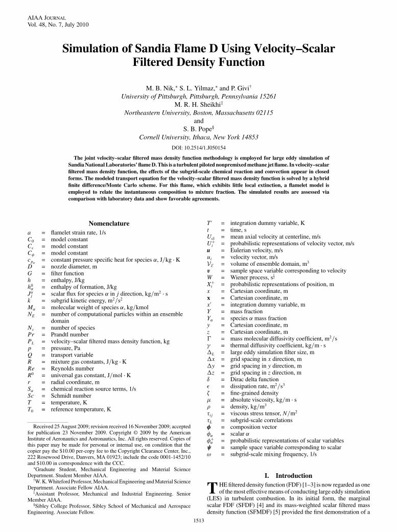
Fig. 3 Axial distribution of the mean filtered temperature at r=D� 0.The symbols denote the experimental data and the solid line denotes the

predicted values.

0 0.5 1 1.5 2 2.50

0.2

0.4

0.6

0.8

<U

>L

/UC

L

r/D

0 0.5 1 1.5 2 2.50

0.05

0.1

0.15

r/D

RM

S (<

U >

L)/

UC

L

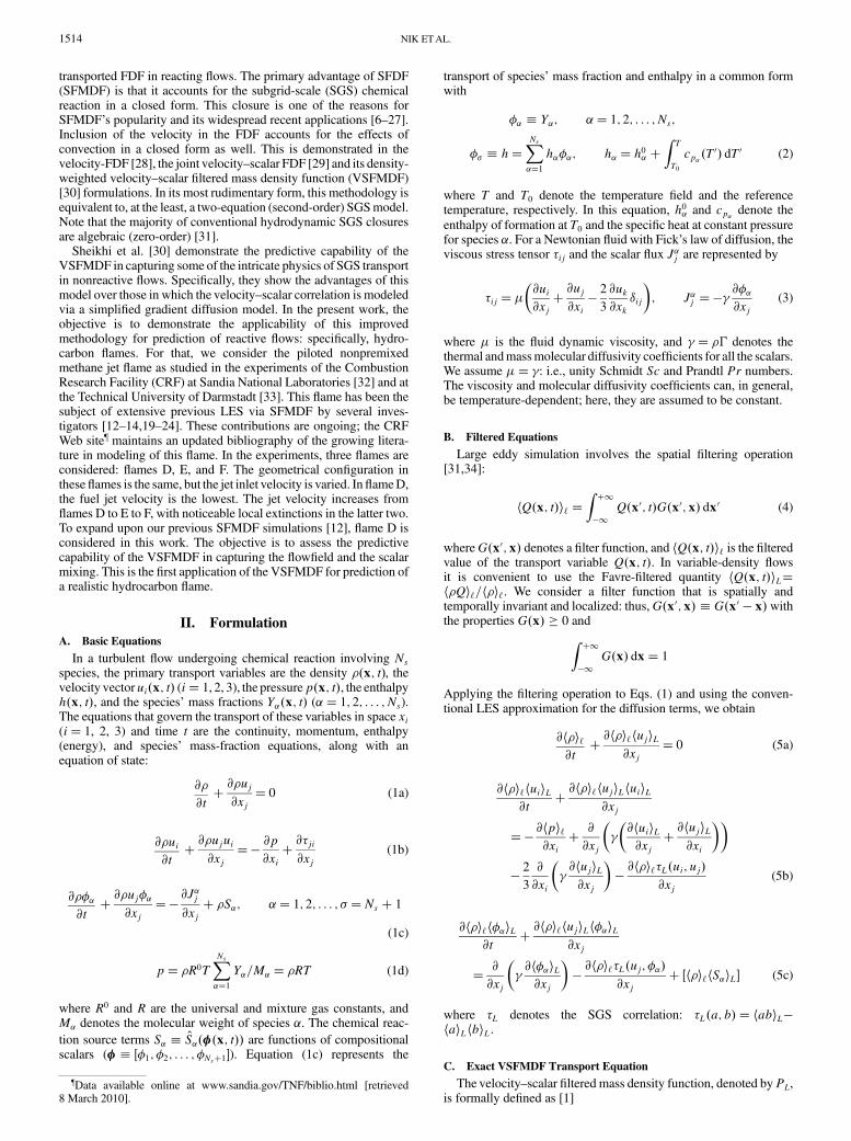
a) b)Fig. 4 Radial distribution of the mean and rms values of the filtered axial velocity. Ucl denotes the mean axial velocity at the centerline at the inlet, the

symbols denote the experimental data. The line denotes the mean value and the thick dashed line denotes the rms value: a) mean axial velocity at

x=D� 15and b) rms value of the axial velocity at x=D� 15.

0 0.5 1 1.5 2 2.50

0.2

0.4

0.6

0.8

1

<φ

>L

r/D

0 1 2 3 40

0.05

0.1

0.15

0.2

r/D

RM

S (<

φ >

L)

a) b)Fig. 5 Radial distribution of the mean and rms values of the filtered mixture fraction. The symbols denote the experimental data. The line denotes the

mean value and the thick dashed line denotes the rms value: a) mean mixture fraction at x=D� 15and b) rms value of the mixture fraction at x=D� 15.

1516 NIK ETAL.

0 0.5 1 1.5 2 2.5

400

600

800

1000

1200

1400

1600<

T>

L

r/D

0 0.5 1 1.5 2 2.50

100

200

300

400

500

r/D

RM

S (<

T >

L)

a) b)Fig. 6 Radial distribution of themean and rms values of thefiltered temperature values. The symbols denote the experimental data. The line denotes the

mean value and the thick dashed line denotes the rms value: a) mean temperature (K) at x=D� 15and b) rms value of the temperature (K) at x=D� 15.

0 0.5 1 1.5 2 2.50

0.05

0.1

0.15

< Y

CH

4 >

L

r/D

0 0.5 1 1.5 2 2.50

0.01

0.02

0.03

0.04

r/D

RM

S (<

YC

H4 >

L)

a) b)Fig. 7 Radial distribution of the mean and rms values of filteredCH4 mass fractions. The symbols denote the experimental data. The line denotes the

mean value and the thick dashed line denotes the rms value: a) meanCH4 mass fraction at x=D� 15and b) rms value ofCH4 mass fraction at x=D� 15.

0 0.5 1 1.5 2 2.5

0.05

0.1

0.15

0.2

0.25

< Y

O2 >

L

r/D

0 0.5 1 1.5 2 2.50

0.01

0.02

0.03

0.04

0.05

0.06

0.07

r/D

RM

S (<

YO

2 >

L)

a) b)Fig. 8 Radial distribution of the mean and rms values of the filteredO2 mass fractions. The symbols denote the experimental data. The line denotes the

mean value and the thick dashed line denotes the rms value: a) mean O2 mass fraction at x=D� 15and b) rms value of O2 mass fraction at x=D� 15.

NIK ETAL. 1517

0 0.5 1 1.5 2 2.50

0.01

0.02

0.03

0.04

< Y

CO

>L

r/D

0 0.5 1 1.5 2 2.50

0.005

0.01

0.015

0.02

r/D

RM

S (<

YC

O >

L)

a) b)

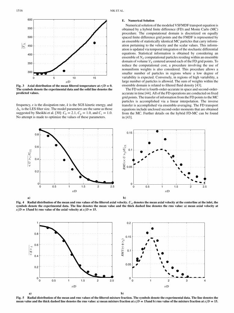
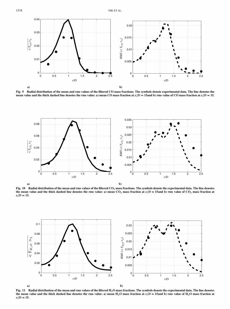
Fig. 9 Radial distribution of the mean and rms values of the filtered CO mass fractions. The symbols denote experimental data. The line denotes the

mean value and the thick dashed line denotes the rms value: a) mean CO mass fraction at x=D� 15and b) rms value of CO mass fraction at x=D� 15.

0 0.5 1 1.5 2 2.50

0.02

0.04

0.06

0.08

< Y

CO

2 >

L

r/D0 0.5 1 1.5 2 2.5

0

0.005

0.01

0.015

0.02

0.025

0.03

0.035

r/D

RM

S (<

YC

O2 >

L)

a) b)Fig. 10 Radial distribution of the mean and rms values of the filteredCO2 mass fractions. The symbols denote the experimental data. The line denotesthe mean value and the thick dashed line denotes the rms value: a) mean CO2 mass fraction at x=D� 15and b) rms value of CO2 mass fraction at

x=D� 15.

0 0.5 1 1.5 2 2.50

0.02

0.04

0.06

0.08

0.1

<Y

H2

O>

L

r/D0 0.5 1 1.5 2 2.5

0

0.005

0.01

0.015

0.02

0.025

0.03

r/D

RM

S (<

YH

2O >

L)

a) b)

Fig. 11 Radial distribution of the mean and rms values of the filteredH2Omass fractions. The symbols denote the experimental data. The line denotes

the mean value and the thick dashed line denotes the rms value: a) mean H2O mass fraction at x=D� 15and b) rms value of H2O mass fraction at

x=D� 15.

1518 NIK ETAL.

III. Flow Configuration and Simulation Parameters

Sandia flame D consists of a main jet with a mixture of 25%methane and 75% air by volume. The nozzle is placed in a coflow ofair and the flame is stabilized by a substantial pilot. The Reynolds

number for themain jet isRe� 22; 400 based on the nozzle diameterD� 7:2 mm and the bulk jet velocity 49:6 m=s.

Simulations are conducted on a three-dimensional Cartesian meshwith uniform spacings in each of the three directions. With availableresources, simulations are affordedwithin a domain spanning 18D �

0.5 0.6 0.7 0.8 0.9 10

2

4

6

8

10

12

14

PD

F

< φ >L

< φ >L

< φ >L

< φ >L

< φ >L

< φ >L

0.4 0.6 0.8 10

1

2

3

4

5

6

7

PD

F

0 0.2 0.4 0.6 0.8 10

1

2

3

4

5

PD

F

0 0.2 0.4 0.6 0.8 10

0.5

1

1.5

2

2.5

3

3.5

PD

F

0 0.2 0.4 0.6 0.8 10

1

2

3

4

PD

F

0 0.2 0.4 0.6 0.8 10

2

4

6

8

10

PD

Fa) b)

c) d)

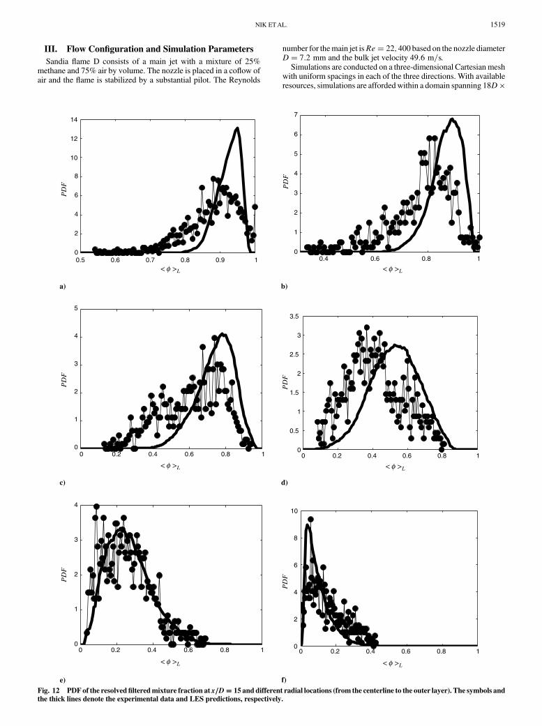
e) f)Fig. 12 PDF of the resolved filteredmixture fraction at x=D� 15 and different radial locations (from the centerline to the outer layer). The symbols and

the thick lines denote the experimental data and LES predictions, respectively.

NIK ETAL. 1519

16D � 16D in the streamwise direction (x) and the two lateraldirections (y and z). The number of grid points are 201 � 161 � 161in the x, y, and z directions, respectively. The filter size is set equal to�L � 2��x�y�z��1=3�, where �x, �y, and �z denote the gridspacings in the corresponding directions. The MC particles aresupplied in the inlet region and are free to move within the domain,due to combined actions of convection and diffusion. The volume ofthe ensemble domain is VE � ��x�y�z� within which NE � 40;threfore, there are at least 200millionMCparticleswithin the domainat all times.

The flow variables at the inflow are set the same as those in theexperiments, including the inlet profiles of the velocity and themixture fraction. The inlet condition for the velocity is presented inFig. 1. The flow is excited by superimposing oscillating axisym-metric perturbations at the inflow. The procedure is similar to that in[45], but the amplitude of forcing is set in such a way to match theexperimentally measured turbulent intensity of the streamwisevelocity at the inlet. Standard characteristic boundary conditions [46]are implemented in all of the FD simulations.

The simulations’ accuracy and the extent of resolved energydepend on the FD grid spacing, the volume of the ensemble domain,the number of MC particles, and the adopted values of the modelconstants. The effects of all of these parameters are investigated in[30]. Per the results of this study, the parameters as selected here yieldan excellent statistical accuracy with minimal dispersion errors.Furthermore, the MC simulation results are monitored to ensure thatthe particles fully encompass and extend well beyond regions ofnonzero vorticity and reaction.

The methane–air reaction mechanism, as occurs in this flame, istaken into account via the flamelet model. This model considers alaminar one-dimensional counterflow (opposed jet) flame config-uration [47]. The detailed kinetics mechanism of the Gas ResearchInstitute (GRI2.11) [48] is employed to describe combustion. Theflamelet table at a strain rate of a� 100 1=s is used to relate thethermochemical variables to the mixture fraction. This value isconsistent with that used in previous SFMDF [12] and probabilitydensity function (PDF) [49] predictions of this flame. It also yieldsthe best overall match of the one-dimensional results with experi-mental data. The predictive capability of VSFMDF is demonstratedby comparing the flow statistics with the Sandia–Darmstadt data[32,33]. These statistics are obtained by long time-averaging of the

filtered field during six flow-through times. The notations �Q andrms�Q� denote, respectively, the time-averaged mean and root-mean-square values of the variableQ. Simulations are conducted on256 processors in conjunction with a message-passing interface andthe PETSc [50–52] library.

IV. Results

For the purpose of flow visualization, the contour plots of FD andMC computations for normalized hRTiL values are shown in Fig. 2.The central jet lies in the middle along the axial coordinate,surrounded by a pilot, where the temperature is the highest andencircled by the air coflow. The region close to inlet is dominated bythe molecular diffusion and the jet exhibits a laminarlike behavior.Further downstream, the growth of perturbations ismanifested by theformation of large-scale coherent vortices. The upstream feedbackfrom the vortices created initially triggers further self-sustainingvortex rollup and subsequent pairing and coalescence of neighboringvortices [53,54]. The slight oscillations inherent in the FD simula-tions due to afixed number of gird points are absent in the Lagrangian(grid-free) results. The streamwise variation of the time-averagedvalues of these results at the centerline is shown in Fig. 3, showingthat the growth of the layer is predicted well.

The capability of the method in predicting the hydrodynamicsfield is demonstrated by examining some of the (reported) radial

(r�����������������z2 � y2

p) distributions of the flow statistics in Fig. 4. The

results at x=D� 15 are shown in this and all of the subsequentfigures, as the profiles at other streamwise location portray similarbehavior for the other statistical quantities considered. TheVSFMDFpredicts the peak value of mean axial velocity profile and the spread

of the jet reasonably well. The rms values, however, are under-predicted. The radial distribution of the mixture fraction is alsoshown to compare well with data (Fig. 5). The mean and rms valuesare close to measured data.

The statistics of the thermochemical variables are also comparedwith corresponding data. The radial distribution of the meantemperature and its corresponding rms values are presented in Fig. 6.Similar to hydrodynamic quantities, the mean profiles showfavorable agreement with measured data, whereas the rms values areunderpredicted at the outer layer. The statistics of the mass fractions(denoted by Y) of several of the species at different streamwiselocations are compared with data in Figs. 7–11. The mean profiles ofthe major species show close agreements with measurements.However, the mean values of the minor species are overpredicted.The rms values show close agreements with measured data at theinner layer, but not as good at the outer layer. These disagreementscan be attributed, in part, to the shortcoming of the flamelet model inrelating the thermochemical variables to the mixture fraction. InFig. 12, the PDFs of the resolvedmixture fraction as predicted by theVSFMDF are compared with those measured experimentally atseveral locations throughout the domain. In general, both the peakand the spreads of the PDFs are predicted well.

V. Conclusions

Since its original development a decade ago, the SFMDF [4,5] hasexperienced widespread applications for LES of a variety of reactingflows [6–8,10,11,13–26,29]. The methodology has found its way inindustry [21] and is now covered as a powerful predictive tool inmostmodern textbooks and handbooks [34,47,55–58]. This popularity ispartially due to the demonstrated capability of themethod to simulaterealistic hydrocarbon flame. The extended methodology, theVSFMDF, is significantly more powerful, as it also accounts for theeffects of SGS convection in an exact manner. This superiority hasbeen previously demonstrated by comparative assessment of themethod in several basic flow configurations [30].

The objective of the present work is to assess the prospects of theVSFMDF for realistic flame simulations. For that, we consider arelatively simple flame: the piloted, nonpremixed, turbulent,methane jet flame (Sandia flame D). For this flame, which waspreviously simulated via SFMDF [12–14,19–24], the thermochem-ical variables are related to themixture fraction via a flamelet table. Amodeled transport equation for the mass-weighted joint FDF of thevelocity and the mixture fraction [30] is considered. This equation issolved by a hybrid finite difference and Monte Carlo method. Thepredictive capability of the overall scheme is assessed by comparisonof the ensemble (long time, Reynolds-averaged) values of thethermochemical variables. It is shown that all of the mean quantitiesare generally predicted well. For the rms values, the predicted valuesagree closely with the experimental data in the inner layer, but not asgood in the outer layer. This discrepancy is attributed, in part, to theuse of the flamelet model in relating all of the thermochemicalvariables to themixture fraction. The PDFs of thismixture fraction aspredicted by the model show very good agreements with data.

Some suggestions for future work are as follows:1) Implement higher-order closures for the generalized Langevin

model parameter Gij [59]. The model parameters considered herecorrespond toRotta’s closure inRANS [34,60].Higher-order closuresimilar to those considered in RANS [39,59] may be implemented.

2) Extend the methodology to account for differential diffusioneffects [23,61–63]. The VSFMDF may be extended to flows withnonunity Prandtl and/or Schmidt numbers. It may also be extended toinclude temperature-dependent viscosity and diffusion coefficients.

3) Quantitatively assess data by performing simulations withdifferent (combination) values for the grid spacings, filter sizes andthe number of MC particles. Such assessments have been previouslydone in SFMDF [18], but require significant more computationalresources for VSFMDF.

4) Extend the methodology for simulation of flames that experi-ence extinction (such as Sandia flames E and F). Such simulationsrequire consideration of finite rate chemistry.

1520 NIK ETAL.

Currently, it is not computationally feasible to implement detailedkinetics in VSFMDF or in SFMDF. Implementation of reduced-kinetics schemes is within reach, provided that sufficient computa-tional resources are available.

Acknowledgments

This work is sponsored byNASAunder grant NNX08AB36A andby the U.S. Air Force Office of Scientific Research with Julian M.Tishkoff as the Program Manager under grant FA9550-06-1-0015.The computations support is provided by the National ScienceFoundation through TeraGrid resources at the Pittsburgh Super-computing Center.

References

[1] Pope, S. B., “Computations of Turbulent Combustion: Progress andChallenges,” Proceedings of the Combustion Institute, Vol. 23, No. 1,1990, pp. 591–612.

[2] Givi, P., “Model Free Simulations of Turbulent Reactive Flows,”Progress in Energy and Combustion Science, Vol. 15, No. 1, 1989,pp. 1–107.doi:10.1016/0360-1285(89)90006-3

[3] Givi, P., “Filtered Density Function for Subgrid-Scale Modeling ofTurbulentCombustion,”AIAA Journal, Vol. 44,No. 1, 2006, pp. 16–23.doi:10.2514/1.15514

[4] Colucci, P. J., Jaberi, F. A., Givi, P., and Pope, S. B., “Filtered DensityFunction for Large Eddy Simulation of Turbulent Reacting Flows,”Physics of Fluids, Vol. 10, No. 2, 1998, pp. 499–515.doi:10.1063/1.869537

[5] Jaberi, F. A., Colucci, P. J., James, S., Givi, P., and Pope, S. B., “FilteredMass Density Function for Large Eddy Simulation of TurbulentReacting Flows,” Journal of Fluid Mechanics, Vol. 401, 1999, pp. 85–121.doi:10.1017/S0022112099006643

[6] Garrick, S. C., Jaberi, F. A., and Givi, P., “Large Eddy Simulation ofScalar Transport in a Turbulent Jet Flow,” Recent Advances in DNS andLES, Vol. 54, edited by D. Knight, and L. Sakell, Kluwer Academic,Dordrecht, The Netherlands, 1999, pp. 155–166.

[7] James, S., and Jaberi, F. A., “Large Scale Simulations of Two-Dimensional Nonpremixed Methane Jet Flames,” Combustion and

Flame, Vol. 123, No. 4, 2000, pp. 465–487.doi:10.1016/S0010-2180(00)00178-4

[8] Zhou, X. Y., and Pereira, J. C. F., “Large Eddy Simulation (2D) of aReacting Plan Mixing Layer Using Filtered Density Function,” Flow,Turbulence and Combustion, Vol. 64, No. 4, 2000, pp. 279–300.doi:10.1023/A:1026595626129

[9] Zhou, X., andMahalingam, S., “AFlame Surface Density BasedModelfor Large Eddy Simulation of Turbulent Nonpremixed Combustion,”Physics of Fluids, Vol. 14, No. 11, 2002, pp. 77–80.doi:10.1063/1.1518691

[10] Heinz, S., “On Fokker-Planck Equations for Turbulent Reacting Flows.Part 2. Filter Density Function for Large Eddy Simulation, Flow,Turbulence and Combustion, Vol. 70, Nos. 1–4, 2003, pp. 153–181.doi:10.1023/B:APPL.0000004934.22265.74

[11] Cha, C.M., and Troullet, P., “ASubgrid-ScaleMixingModel for Large-Eddy Simulations of Turbulent Reacting Flows Using the FilteredDensity Function,” Physics of Fluids, Vol. 15, No. 6, 2003, pp. 1496–1504.doi:10.1063/1.1569920

[12] Sheikhi, M. R. H., Drozda, T. G., Givi, P., Jaberi, F. A., and Pope, S. B.,“Large Eddy Simulation of a Turbulent Nonpremixed Piloted MethaneJet Flame (Sandia Flame D),” Proceedings of the Combustion Institute,Vol. 30, No. 1, 2005, pp. 549–556.doi:10.1016/j.proci.2004.08.028

[13] Raman, V., Pitsch, H., and Fox, R. O., “Hybrid Large-Eddy Simulation/Lagrangian Filtered Density Function Approach for SimulatingTurbulent Combustion,” Combustion and Flame, Vol. 143, Nos. 1–2,2005, pp. 56–78.doi:10.1016/j.combustflame.2005.05.002

[14] Raman, V., and Pitsch, H., “Large-Eddy Simulation of a Bluff-Body-Stabilized Nonpremixed Flame Using a Recursive Filter-RefinementProcedure,” Combustion and Flame, Vol. 142, No. 4, 2005, pp. 329–347.doi:10.1016/j.combustflame.2005.03.014

[15] van Vliet, E., Derksen, J. J., and van den Akker, H. E. A., “TurbulentMixing in a Tubular Reactor: Assessment of an FDF/LES Approach,”

AIChE Journal, Vol. 51, No. 3, 2005, pp. 725–739.doi:10.1002/aic.10365

[16] Carrara,M. D., andDesJardin, P. E., “AFilteredMass Density FunctionApproach to Modeling Separated Two-Phase Flows Using LES I:Mathematical Formulation,” International Journal ofMultiphase Flow,Vol. 32, No. 3, 2006, pp. 365–384.doi:10.1016/j.ijmultiphaseflow.2005.11.003

[17] Mustata, R., Valĩno, L., Jiménez, C., Jones, W. P., and Bondi, S., “AProbability Density Function Eulerian Monte Carlo Field Method forLarge Eddy Simulations: Application to a Turbulent Piloted Methane/Air Diffusion Flame (Sandia d),” Combustion and Flame, Vol. 145,Nos. 1–2, 2006, pp. 88–104.doi:10.1016/j.combustflame.2005.12.002

[18] Drozda, T. G., Sheikhi, M. R. H., Madnia, C. K., and Givi, P.,“Developments in Formulation and Application of the Filtered DensityFunction,” Flow, Turbulence and Combustion, Vol. 78, No. 1, 2007,pp. 35–67.

[19] Jones, W. P., Navarro-Martinez, S., and Röhl, O., “Large EddySimulation of Hydrogen Auto-Ignition with a Probability DensityFunction Method,” Proceedings of the Combustion Institute, Vol. 31,No. 2, 2007, pp. 1765–1771.doi:10.1016/j.proci.2006.07.041

[20] Jones, W. P., and Navarro-Martinez, S., “Large Eddy Simulation ofAutoignition with a Subgrid Probability Density Function Method,”Combustion and Flame, Vol. 150, No. 3, 2007, pp. 170–187.doi:10.1016/j.combustflame.2007.04.003

[21] James, S., Zhu, J., and Anand, M. S., “Large Eddy Simulations ofTurbulent Flames Using the Filtered Density Function Model,”Proceedings of the Combustion Institute, Vol. 31, No. 2, 2007,pp. 1737–1745.doi:10.1016/j.proci.2006.07.160

[22] Chen, J. Y., “A Eulerian PDF Scheme for LES of NonpremixedTurbulent Combustion with Second-Order-Accurate Mixture Frac-tion,” Combustion Theory and Modelling, Vol. 11, No. 5, 2007,pp. 675–695.doi:10.1080/13647830601091723

[23] McDermott, R., and Pope, S. B., “A Particle Formulation for TreatingDifferential Diffusion in Filtered Density Function Methods,” Journalof Computational Physics, Vol. 226, No. 1, 2007, pp. 947–993.doi:10.1016/j.jcp.2007.05.006

[24] Raman, V., and Pitsch, H., “A Consistent LES/Filtered-DensityFunction Formulation for the Simulation of Turbulent Flames withDetailed Chemistry,” Proceedings of the Combustion Institute, Vol. 31,No. 2, 2007, pp. 1711–1719.doi:10.1016/j.proci.2006.07.152

[25] Afshari, A., Jaberi, F. A., and Shih, T.I. P., “Large-Eddy Simulations ofTurbulent Flows in an Axisymmetric Dump Combustor,” AIAA

Journal, Vol. 46, No. 7, 2008, pp. 1576–1592.doi:10.2514/1.25467

[26] Drozda, T. G., Wang, G., Sankaran, V., Mayo, J. R., Oefelein, J. C., andBarlow,R. S., “Scalar FilteredMassDensity Functions inNonpremixedTurbulent Jet Flames,” Combustion and Flame, Vol. 155, Nos. 1–2,2008, pp. 54–69.doi:10.1016/j.combustflame.2008.06.012

[27] Givi, P., Sheikhi, M. R. H., Drozda, T. G., and Madnia, C. K., “LargeScale Simulation of Turbulent Combustion,” Combust. Plasma Chem.,Vol. 6, No. 1, 2008, pp. 1–9.

[28] Gicquel, L. Y. M., Givi, P., Jaberi, F. A., and Pope, S. B., “VelocityFiltered Density Function for Large Eddy Simulation of TurbulentFlows,” Physics of Fluids, Vol. 14, No. 3, 2002, pp. 1196–1213.doi:10.1063/1.1436496

[29] Sheikhi, M. R. H., Drozda, T. G., Givi, P., and Pope, S. B., “Velocity-Scalar Filtered Density Function for Large Eddy Simulation ofTurbulent Flows,” Physics of Fluids, Vol. 15, No. 8, 2003, pp. 2321–2337.doi:10.1063/1.1584678

[30] Sheikhi, M. R. H., Givi, P., and Pope, S. B., “Velocity-Scalar FilteredMass Density Function for Large Eddy Simulation of TurbulentReacting Flows,”Physics of Fluids, Vol. 19, No. 9, 2007, Paper 095106.doi:10.1063/1.2768953

[31] Sagaut, P., Large Eddy Simulation for Incompressible Flows, 3rd ed.,Springer–Verlag, New York, 2005.

[32] Nooren, P. A., Versiuis, M., Van der Meer, T. H., Barlow, R. S., andFrank, J. H., “Raman-Rayleigh-LIFMeasurements of Temperature andSpecies Concentrations in the Delft Piloted Turbulent Jet DiffusionFlame,” Applied Physics B (Lasers and Optics), Vol. 71, No. 1, 2000,pp. 95–111.doi:10.1007/s003400000278

[33] Schneider, C., Dreizler, A., Janicka, J., and Hassel, E. P., “Flow Field

NIK ETAL. 1521

Measurements of Stable and Locally Extinguishing Hydrocarbonfu-elled Jet Flames, Combustion and Flame, Vol. 135, No. 1, 2003,pp. 185–190.doi:10.1016/S0010-2180(03)00150-0

[34] Pope, S. B., Turbulent Flows, Cambridge Univ. Press, Cambridge,England, U.K., 2000.

[35] O’Brien, E. E., “The Probability Density Function (PDF) Approach toReacting Turbulent Flows,” edited by P. A. Libby, and F. A. Williams,Turbulent Reacting Flows, Vol. 44, Springer–Verlag, Heidelberg, 1980,Chap. 5, pp. 185–218.

[36] Pope, S. B., “PDFMethods for Turbulent Reactive Flows,” Progress inEnergy and Combustion Science, Vol. 11, No. 2, 1985, pp. 119–192.doi:10.1016/0360-1285(85)90002-4

[37] Vreman, B., Geurts, B., and Kuerten, H., “Realizability Conditions forthe Turbulent Stress Tensor in Large-Eddy Simulation,” Journal of

Fluid Mechanics, Vol. 278, 1994, pp. 351–362.doi:10.1017/S0022112094003745

[38] Karlin, S., and Taylor, H.M.,A Second Course in Stochastic Processes,Academic Press, New York, 1981.

[39] Haworth, D. C., and Pope, S. B., “A Generalized Langevin Model forTurbulent Flows,”Physics of Fluids, Vol. 29, No. 2, 1986, pp. 387–405.doi:10.1063/1.865723

[40] Dreeben, T. D., and Pope, S. B., “Probability Density Function andReynolds-Stress Modeling of Near-Wall Turbulent Flows,” Physics ofFluids, Vol. 9, No. 1, 1997, pp. 154–163.doi:10.1063/1.869157

[41] Wax, N., Selected Papers on Noise and Stochastic Processes, Dover,New York, 1954.

[42] Gardiner, C. W., Handbook of Stochastic Methods, Springer–Verlag,New York, 1990.

[43] Madnia, C. K., Jaberi, F. A., and Givi, P., “Large Eddy Simulation ofHeat andMass Transport in Turbulent Flows,”Handbook of NumericalHeat Transfer, 2nd. ed., Wiley, New York, 2006, Ch. 5, pp. 167–189.

[44] Kennedy, C. A., and Carpenter, M. H., “Several New NumericalMethods for Compressible Shear-Layer Simulations,” Applied

Numerical Mathematics, Vol. 14, No. 4, 1994, pp. 397–433.doi:10.1016/0168-9274(94)00004-2

[45] Danaila, I., and Boersma, B. J., “Direct Numerical Simulation ofBifurcating Jets,” Physics of Fluids, Vol. 12, No. 5, 2000, pp. 1255–1257.doi:10.1063/1.870377

[46] Poinsot, T. J., and Lele, S. K., “Boundary Conditions for DirectSimulations of Compressible Viscous Flows,” Journal of Computa-

tional Physics, Vol. 101, No. 1, 1992, pp. 104–129.doi:10.1016/0021-9991(92)90046-2

[47] Peters, N., Turbulent Combustion, Cambridge Univ. Press, Cambridge,England, U.K., 2000.

[48] GRI-Mech, Software Package, Ver. 3.0, http://www.me.berkeley.edu/gri_mech, Gas Research Inst., Chicago, IL.

[49] Muradoglu, M., Liu, K., and Pope, S. B., “PDF Modeling of a Bluff-Body Stabilized Turbulent Flame,” Combustion and Flame, Vol. 132,Nos. 1–2, 2003, pp. 115–137.doi:10.1016/S0010-2180(02)00430-3

[50] PETSc: Portable, Extensible Toolkit for Scientific Computation,Software Package, Ver. 3.0.0, MSD Div., Argonne National Lab.,Argonne, IL, 2008, http://www.mcs.anl.gov/petsc [retrieved8 March 2010].

[51] PETSc Users Manual, Argonne National Lab., TR ANL-95/11, Rev.2.1.5, Argonne, IL, 2004.

[52] Balay, S., Gropp, W. D., McInnes, L. C., and Smith, B. F., “EfficientManagement of Parallelism in Object Oriented Numerical SoftwareLibraries,Modern Software Tools in Scientific Computing, edited by E.Arge, A. M. Bruaset, and H. P. Langtangen, Birkhäuser, Boston, 1997,pp. 163–202.

[53] Givi, P., and Riley, J. J., “Some Current Issues in the Analysis ofReacting Shear Layers: Computational Challenges,” Major Research

Topics in Combustion, edited by M. Y. Hussaini, A. Kumar, and R. G.Voigt, Springer–Verlag, New York, 1992, pp. 588–650.

[54] Drummond, J. P., and Givi, P., “Suppression and Enhancement ofMixing in High-Speed Reacting Flow Fields,” Combustion in High-

Speed Flows, edited by J. D. Buckmaster, T. L. Jackson, and A. Kumar,Kluwer Academic, Dordrecht, The Netherlands, 1994, pp. 191–229.

[55] Bilger, R. W., “Future Progress in Turbulent Combustion Research,”Progress in Energy and Combustion Science, Vol. 26, Nos. 4–6, 2000,pp. 367–380.doi:10.1016/S0360-1285(00)00015-0

[56] Fox, R. O., Computational Models for Turbulent Reacting Flows,Cambridge Univ. Press, Cambridge, England, U.K., 2003.

[57] Heinz, S., “On Fokker-Planck Equations for Turbulent Reacting Flows.Part 2. Filtered Density Function for Large Eddy Simulation,” Flow,

Turbulence and Combustion, Vol. 70, Nos. 1–4, 2003, pp. 153–181.doi:10.1023/B:APPL.0000004934.22265.74

[58] Minkowycz, W. J., Sparrow, E. M., and J. Y. Murthy, Handbook of

Numerical Heat Transfer, 2nd ed., Wiley, New York, 2006.[59] Pope, S. B., “On the Relation Between Stochastic Lagrangian Models

of Turbulence and Second-MomentClosures,”Physics of Fluids, Vol. 6,No. 2, 1994, pp. 973–985.doi:10.1063/1.868329

[60] Wilcox, D. C., Turbulence Modeling for CFD, DCW Industries, LaCãnada, CA, 1993.

[61] Jaberi, F. A., Miller, R. S., Mashayek, F., and Givi, P., “DifferentialDiffusion in Binary Scalar Mixing and Reaction,” Combustion and

Flame, Vol. 109, No. 4, 1997, pp. 561–577.doi:10.1016/S0010-2180(97)00045-X

[62] Kerstein, A. R., Cremer, M. A., and McMurtry, P. A., “ScalingProperties of Differential Molecular Diffusion Effects in Turbulence,”Physics of Fluids, Vol. 7, No. 8, 1995, pp. 1999–2007.doi:10.1063/1.868511

[63] Yeunga, P. K., Xu, S., and Sreenivasan,K. R., “Schmidt Number Effectson Turbulent Transport with Uniform Mean Scalar Gradient,” Physicsof Fluids, Vol. 14, No. 12, 2002, pp. 4178–4191.doi:10.1063/1.1517298

T. JacksonAssociate Editor

1522 NIK ETAL.