SIMULATION OF TORNADO-GENERATED MISSILES by DIA AREF MALAEB, B.S. IN C.E. A THESIS IN CIVIL ENGINEERING Submitted to the Graduate Faculty of Texas Tech University in Partial Fulfillment of the Requirements for the Degree of MASTER OF SCIENCE IN CIVIL ENGINEERING Approved Accepted ,) December, 198()'
Transcript
SIMULATION OF TORNADO-GENERATED MISSILES
by
DIA AREF MALAEB, B.S. IN C.E.
A THESIS
IN
CIVIL ENGINEERING
Submitted to the Graduate Faculty of Texas Tech University in
Partial Fulfillment of the Requirements for
the Degree of
MASTER OF SCIENCE
IN
CIVIL ENGINEERING
Approved
Accepted
,) December, 198()'
ACKNOWLEDGEMENTS
r. -·:' ._..,·!'I . ....-<-The author wishes to express his deep appreciation to Dr. James
R. McDonald for his patience, guidance and valuable assistance through
out this research effort. The support provided for the conduct of
this research by the Nuclear Regulatory Commission, by the Department
of Civil Engineering at Texas Tech University, and by the Institute
for Disaster Research at Texas Tech University is also acknowledged.
Drs. :<i shor C. Mehta and Joseph E. Minor are gratefully acknowledged
for their helpful criticisms and recommendations.
i i
CONTENTS
ACKNOWLEDGEMENTS
LIST OF TABLES
LIST OF FIGURES
I. INTRODUCTION
A. Objectives
B. Research Plan
II. REVIEW OF PREVIOUS RESEARCH
A. Previous Tornado Missile Trajectory Models
1. Wind Field Model
2. Aerodynamic Flight Parameter
3. Initial Conditions
4. Number of Degrees of Freedom
B. Basis for Rational Approach
1. Wind Field Model
2. Aerodynamic rlight Parameter
3. Initial Conditions
4. Number of Degrees of Freedom
C. Summary of Desired Trajectory Model Features
III. MISSILE TRAJECTORY MODEL
A. Wind Field r~odel
B. Missile Characteristics
C. Initial Conditions
D. Equations of Motion
i i i
Paoe ___..........,_
ii
v
vi
1
3
3
5
6
7
9
11
12
12
1 3
14
15
17
17
19
19
24
27
28
E . N wne r i c a l Sol u t ion
F. Computer Code
IV. COMPARISON OF SIMULATION STUDY WITH OBSERVED MISSILE BEHAVIOR
A. Approach
B. Bossier City Tornado
l. Damage Observations at Meadowview Elementary School
2. Fujita•s Analysis of Tornado Wind field
C. Factors Affecting Trajectory Path
D. Case Studies
1. Controlling Parameters
2. Trajectories Based on Fujita•s Analysis of Wind Fi~ld
E. Conclusions Based on Simulation Studies
V. SUMMARY AND CONCLUSIONS
A. Summary
B. Conclusions
LIST OF REFERENCES
iv
31
32
37
37
37
38
49
49
59
39
66
68
73
73
74
75
Table
1
2
3
4
5
6
7
8
9
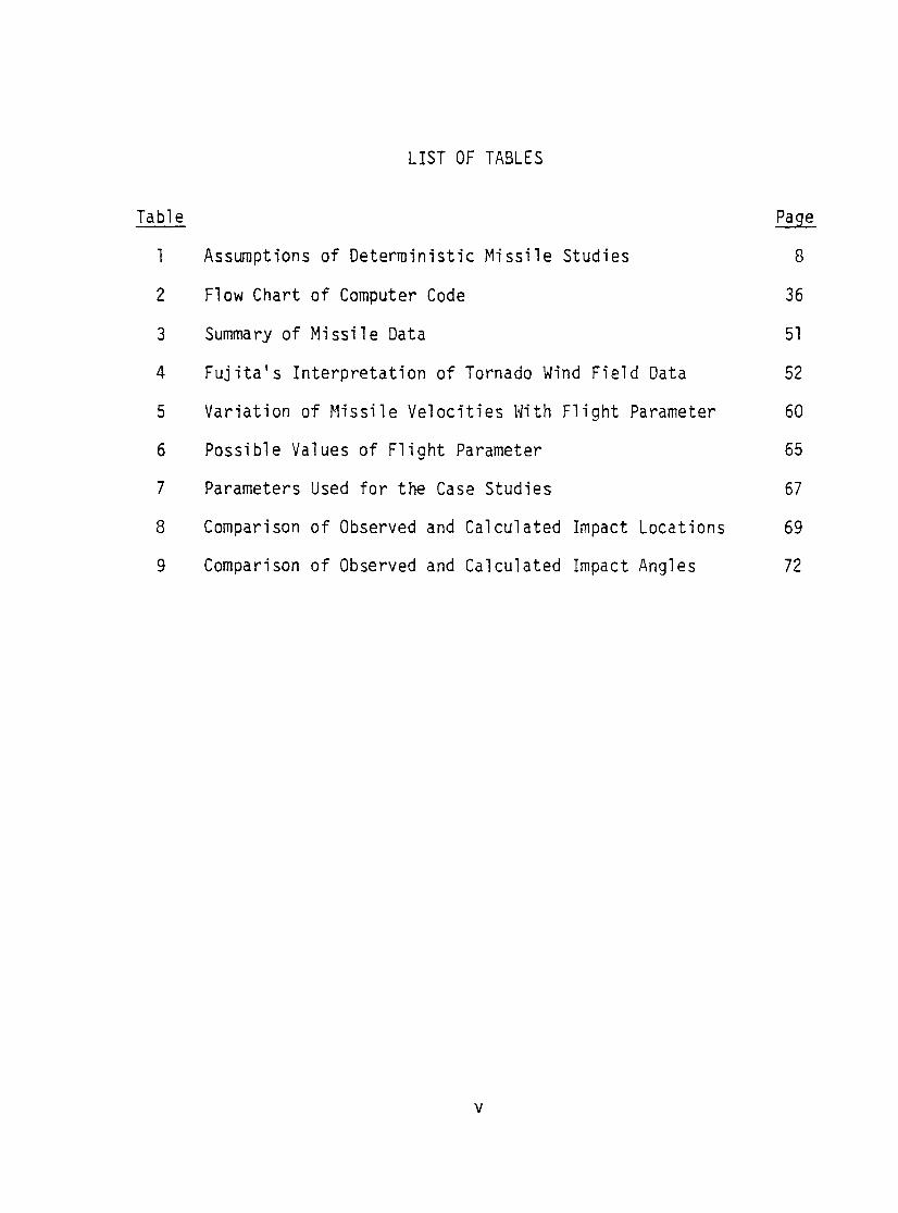
LIST OF TABLES
Assumptions of Deterministic Missile Studies
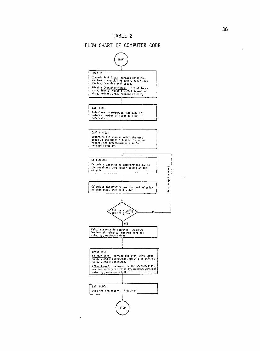
Flow Chart of Computer Code
Summary of Missile Data
Fujita's Interpretation of Tornado Wind Field Data
Variation of Missile Velocities With Flight Parameter
Possible Values of Flight Parameter
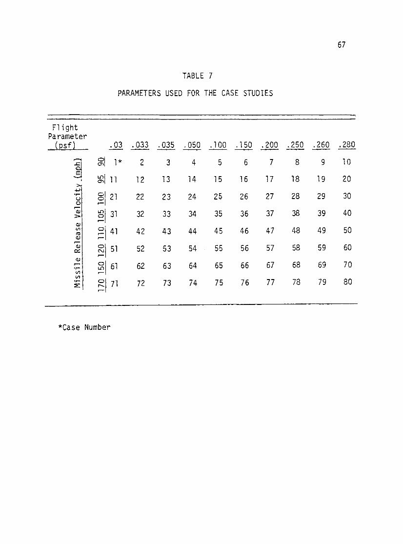
Parameters Used for the Case Studies
Comparison of Observed and Calculated Impact Locations
Comparison of Observed and Calculated Impact Angles
v
Page
8
36
51
52
60
65
67
69
72
Figure
1
2
3
4
5
6
7
8
9
10
11
12
13
14
15
16
17
LIST OF FIGURES
Schematic Diagram of Single Vortex Tornado Model - DBT-77
Definition of Crossing Angle
Variation of Drag Coefficient with Orientation of Missile
Definition of Angles s and e
Tornado Damage in Vicinity of Meadowview Elementary School (Fujita, 1979)
Tornado Damage at Meadowview Elementary School
Typical Exterior Wall at Elementary School
Typical Beam-to-Column Connections at Roof
Roof Cross Section at Exterior Wall
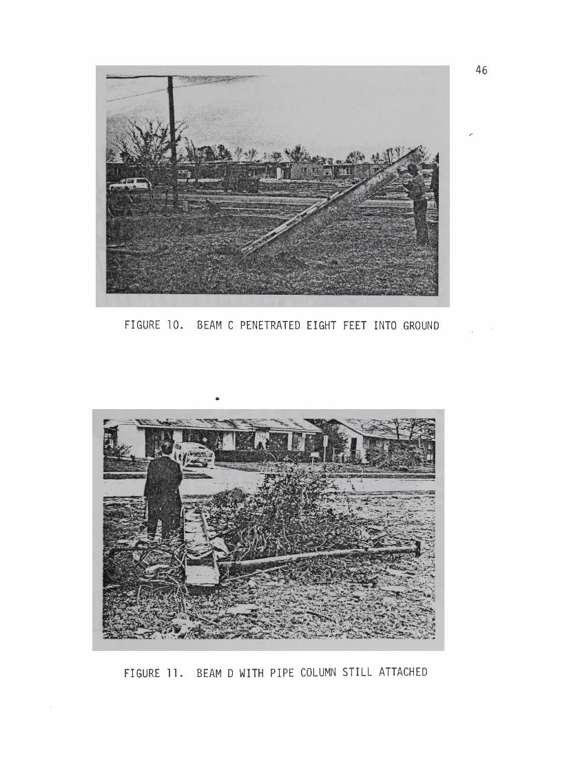
Beam C Penetrated Eight Feet Irito Ground
Beam D With Pipe Column Still Attached
Beam D at Point of Impact After Passing Through Corner of House
Beam E With the Pipe Column Still Attached
Beam F Struck Roof of House Located 1000 Ft From School Building
Isovels of Tornadic Wind Speed as Interpreted By Fujita
Effect of Release Velocity on Missile Trajectory When Missile is Located to Left of Path
Effect of Release Velocity on ~issile Trajectory When Missile is Located to Right of Path
vi
21
23
26
29
39
40
42
43
44
46
46
47
48
48
50
54
56
LIST OF FIGURES (Cont'd.)
Figure
18 Missile Position Relative to Tornado Position When Missile is Released on Back Side of Tornado Core 57
19 Missile Position Relative to Tornado Position When Missile is Released on Front Side of Tornado Core 58
20 Variation of Missile Velocities With Values of Flight Parameters 61
21 Uplift Forces Required to Cause Column Anchorage Failure 63
22 Calculated Missile Trajectories and Observed Impact Points 70
vii
I. INTRODUCTION
The destructive damage caused by tornadoes in the United States
and in other countries such as Australia and Japan is receiving more
attention from engineers and managers each year. Responsible author-
ities are realizing that dollars invested in tornado protection pay
handsome dividends in safety, productivity, and damage mitigation
should that facility be struck by a tornado.
Damage caused by tornadoes is produced by three basic types of
forces:
1) wind induced forces,
2) atmospheric pressure change induced forces, and
3) impactive forces from windborne debris.
The research reported herein deals with the nature and characteristics
of the items picked up and transported by tornadic winds, i.e. tornado-
generated missiles.
Federal law* requires that structures that house equipment vital
to the safe shutdown of a nuclear power reactor shall be designed to
withstand the effects of natural phenomena, including tornadoes. The
spirit of this law has been applied to other facilities that
house nuclear materials, which, if released to the atmosphere, could
cause injury to people and damage to the environment. Such structures
*Policy and Regulatory Practice Governing the Siting of Nuclear Power Reactors [10 CFR Part 50].
must be designed to withstand certain types of potential missiles,
which are consistent with an acceptable risk level.
2
Hospitals, fire stations and conventional power plants should be
able to function after a tornado event. They, too, may require design
considerations for protection from tornado-generated missiles. Shel
ters for the protection of people in residences, schools and other
public buildings should also be designed to withstand impact from
tornado-generated missiles. Regardless of the degree of tornado pro
tection, the designer of a facility is faced with the so-called 11 tor
nado missile 11 problem. He needs to know the types of missiles that
are transported by tornadoes, their trajectory characteristics, and
the impactive effect on walls and the roof of his building. Thus, the
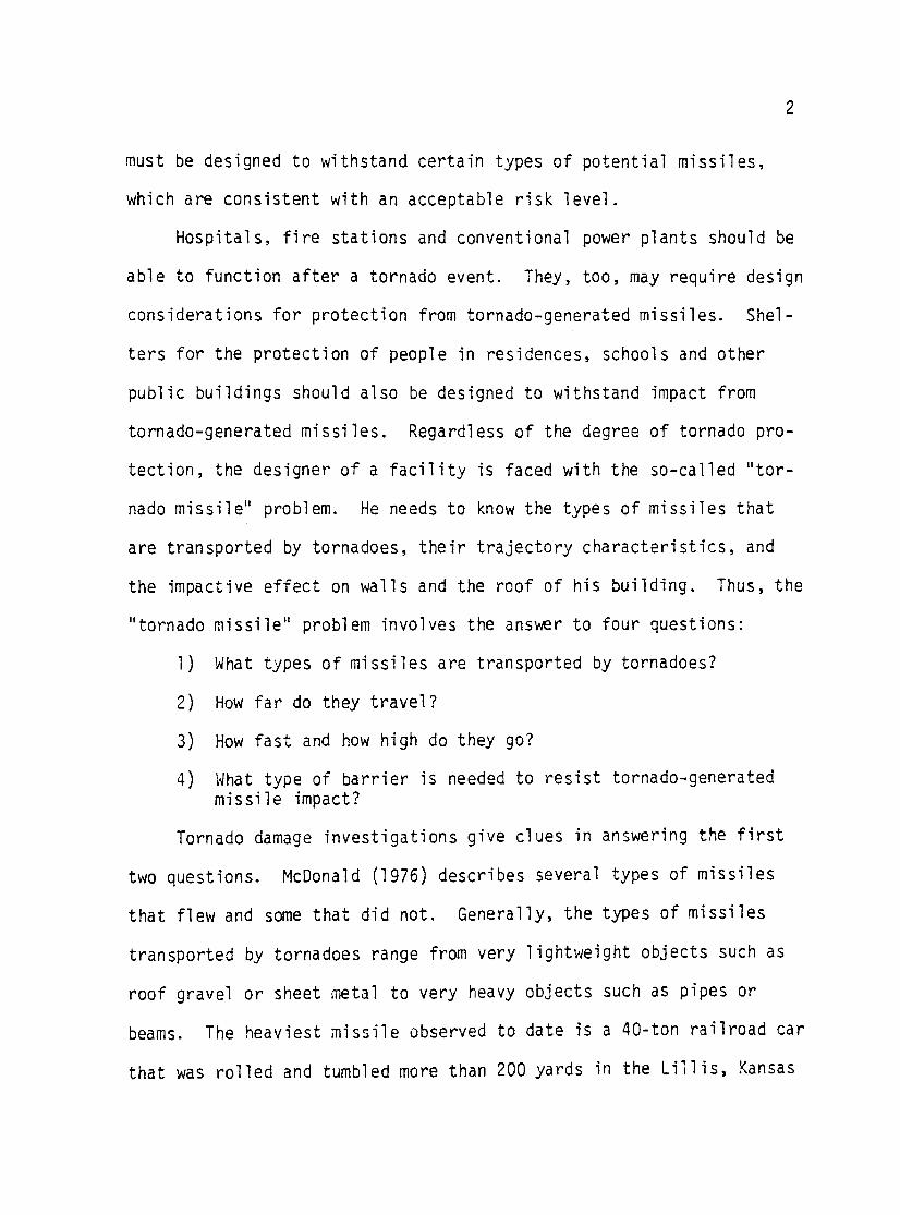
11 tornado mi ssil e 11 prob 1 em invo 1 ves the answer to four questions:
1) What types of missiles are transported by tornadoes?
2) How far do they travel?
3) How fast and how high do they go?
4) What type of barrier is needed to resist tornado-generated missile impact?
Tornado damage investigations give clues in answering the first
two questions. McDonald (1976) describes several types of missiles
that flew and some that did not. Generally, the types of missiles
transported by tornadoes range from very lightweight objects such as
roof gravel or sheet metal to very heavy objects such as pipes or
beams. The heaviest missile observed to date is a 40-ton railroad car
that was rolled and tumbled more than 200 yards in the Lillis, Kansas
3
tornado of 1978. (Incident is documented in tornado damage files of
the Institute for Disaster Research, Texas Tech University.) The dis-
tance traveled by a missile can be determined from field investigations,
provided its origin can be identified.
The answer to the third question is more difficult, since it is
almost impossible to obtain data on the missile trajectories themselves.
Photogrammetric analysis of movie films showing missile flights is one
possibility, but these films are rare. Indirect methods such as com-
puter simulation are the only alternatives available. Barrier analy-
sis and design involved with the fourth question are beyond the scope
of this project.
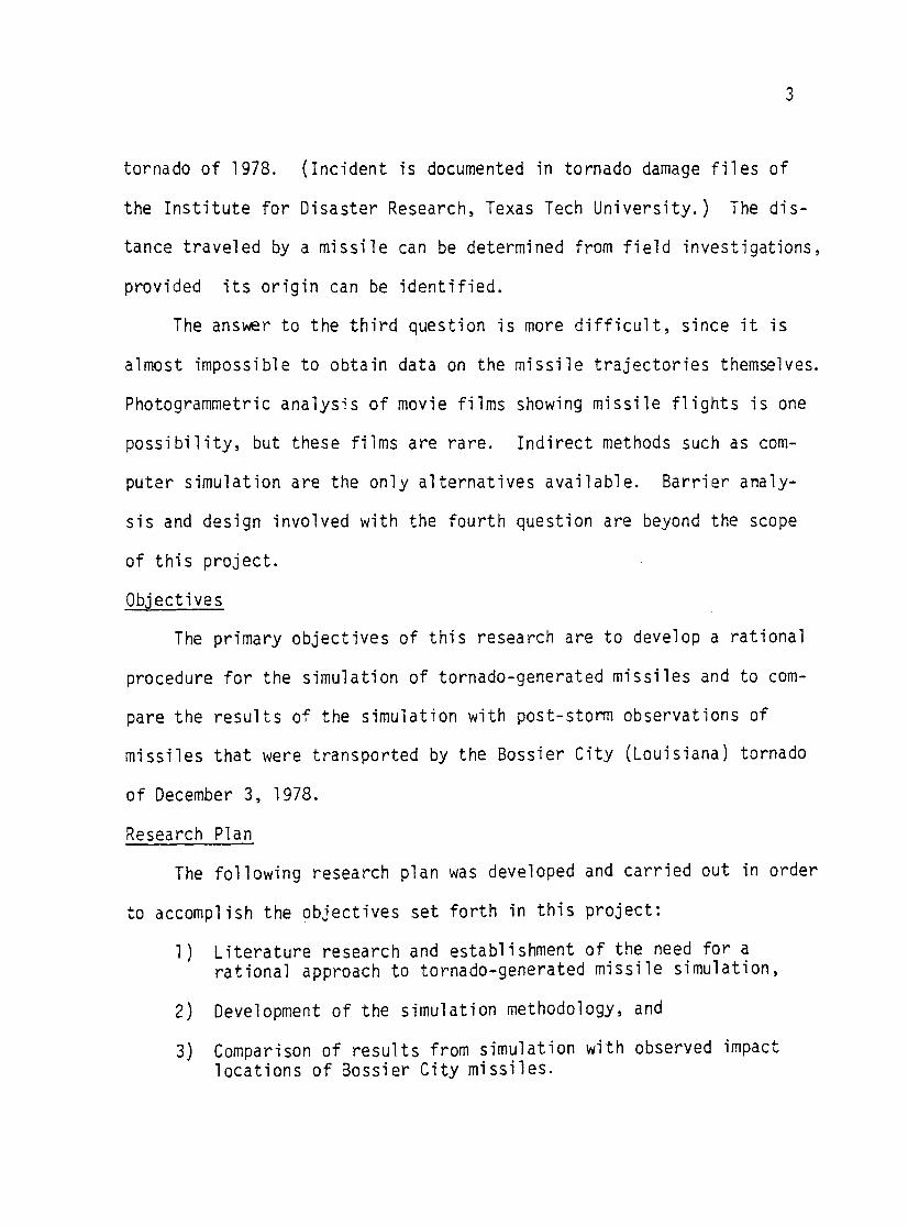
Objectives
The primary objectives of this research are to develop a rational
procedure for the simulation of tornado-generated missiles and to com
pare the results of the simulation with post-storm observations of
missiles that were transported by the Bossier City (Louisiana) tornado
of December 3, 1978.
Research Plan
The following research plan was developed and carried out in order
to accomplish the objectives set forth in this project:
1 )
2)
3)
Literature research and establishment of the need for a rational approach to tornado-generated missile simulation,
Development of the simulation methodology, and
Comparison of results from simulation with observed impact locations of Bossier City missiles.
4
Numerous attempts can be found in the literature to simulate or,
by some means, calculate tornado-generated missile trajectories.
Diverse results have been obtained because each researcher used a dif
ferent set of assumptions or conditions. Review of previous work is
presented with the objective of sorting out the different parameters
affecting trajectory characteristics. Once the various published
attempts at missile trajectory calculations are reviewed, the need for
a rational approach is obvious.
The simulation methodology involves selection of an appropriate
tornado wind field model, identification of significant missile char
acteristics, establishment of appropriate initial conditions, and
development of an appropriate computer code to perform the dynamic
trajectory calculations. •
A somewhat circumstantial approach to verification of the trajec
tory methodology is used. An attempt is made to simulate the trajec
tories of six steel wide flange beams that were transported by the
Bossier City tornado. Certain parameters relating to the tornado wind
field and missile characteristics are varied within a plausible range
to obtain trajectories that match the initial location and impact
position of the missiles.
II. REVIEW OF PREVIOUS RESEARCH
There have been numerous attempts to simulate tornado missile
trajectories. Almost all such efforts have been related to satisfying
licensing requirements for nuclear power plants. Other applications
of missile technology have been spinoffs from the nuclear power indus-
try.
To date, three basic approaches have used to gain an understand
ing of missile behavior:
1) a purely probabilistic, rather than deterministic, assessment of the missile problem;
2} Monte Carlo simulation of missile transport at a site specific location; and
3) establishment of a list of generic missiles by deterministic methods.
The first approach attempts to quantify the various probabilities
associated with an event that involves the occurrence of a tornado,
the presence of potential missiles in the tornado path, the accelera-
tion of the nissile to a velocity sufficient to cause damage, and the
impact of this missile at a critical point on the buiiding. To date,
no one has been able to quantify all of these probabilities to the
satisfaction of licensing authorities, although Meyer and Morrow (1975)
did try. Consideration of this approach is beyond the scope of this
research.
The second approach has not been used as a practical procedure
for design, but has been used as a research tool to study the missile
5
6
from a probabilistic point of view. Johnson and Abbott (1976) per
formed the equivalent of 10 million years of missile simulation by
passing randomly selected tornadoes over an idealization of the power
reactor site. All potential missiles were catalogued from an on-site
inspection. The computer code then calculated missile trajectories
as randomly selected tornadoes were passed over the site and recorded
strikes on the safety-related facilities. The probabilities of missile
strikes were then calculated. The amount of effort and computer time
required to generate the data is not practical for general design pur-
poses.
The third approach has been used by the NRC as a part of the
licensing procedure for nuclear power plants (Ref. NRC, 1975).
A list of generic missiles was somewhat arbitrarily selected by the
NRC licensing staff. Most previous work with tornado-generated mis
siles has been with the objective to prove or disprove the correct
ness of the NRC generic missile list. The list has been revised from
time to time, but still lacks justification based on a definitive
study of tornado missiles.
Previous Tornado Missile Trajectory Models
The methodology, including assumptions and calculation procedures,
is referred to herein as a missile trajectory model. Given certain
information about the tornado wind field and the missile characteris
tics, the model (usually in the form of a computer code) gives infor
mation about missile acceleration, velocity, and displacement as a
7
function of time. This type of model provides deterministic, rather
than probabilistic, information about the missile. Table 1 lists the
deterministic missile studies that have been conducted since the first
one was performed by Bates and Swanson in 1967.
The basic differences in the various models involve assumptions
regarding
1) \Jind field model,
2) flight parameter,
3) initial conditions, and
4) degrees of freedom of dynamic model.
The assumptions relating to the above four factors by each different
methodology are also given in Table 1.
Wind Field Model
Bates and Swanson (1967) used the analysis of Hoecker (1960) to
develop a wind field model of a tornado. The maximum wind speed of
the Dallas tornado was scaled to a value of 360 mph. Other methodol
ogies used slightly modified forms of the Bates and Swanson wind field
model (Paddleford, 1969; Lee, 1973; James, et al. 1974; Iotti, 1975).
The original Bates and Swanson model did not encompass all of space
around the tornado core. Later models identified wind flow in all of
space and established bounds on maximum tornadic windspeeds.
Bhattaharyya (1975) used a wind field model proposed by Kuo (1971).
While Kuo's model has a more rigorous fluid dynamic basis than the model
developed by Hoecker (1960), it is not convenient to use from an
TABL
E 1
ASSU
MPT
IONS
OF DETERMINI~TIC
MIS
SILE
STU
DIES
Win
d F
ield
Mod
el
Fli
ght
Para
met
er
Init
ial
De9
rees
0-
f R
efer
ence
Y
ear
Bas
ed O
n B
ased
On
Con
diti
ons
Free
dom
Date~ an
d Sw
anso
n 19
67
Hoe
cker
' s ~
lode
1
Eff
ecti
ve A
rea
Thr
ee
Inje
ctio
n 3
(Tum
blin
g)
Mod
es
Pad
dlef
ord
1969
H
oeck
er's
Mod
el E
ffec
tive
Are
a In
itia
l E
leva
tion
3
(Tum
blin
g)
Lee
1973
H
oeck
er's
Mod
el E
ffec
tive
Are
a Im
puls
ive
Inje
ctio
n 3
(Tum
blin
g)
Jam
es,
et a
l.
1974
H
oeck
er's
Mod
el E
ffec
tive
Are
a T
hree
In
ject
ion
3 (T
umbl
ing)
Oha
ttach
aryy
a 19
75
Kuo
' s M
odel
Max
i mum
Are
a (N
on-T
umbl
ing)
In
itia
l E
leva
tion
3
Iott
i 19
75
Hoe
cker
's M
odel
Eff
ecti
ve A
rea
Exp
losi
ve
Inje
ctio
n 3
(Tum
blin
g)
Bee
th a
nd
Hob
bs
1975
C
ombi
ned
Ran
kine
E
ffec
tive
Val
ue
Init
ial
Ele
vati
on
3 V
orte
x (T
urub
ling)
Mey
er a
nd
Mor
row
19
7S
Com
bine
d R
anki
ne
Eff
ecti
ve V
alue
In
itia
l E
leva
tion
3
Vor
tex
(Tum
blin
g)
Sirn
iu a
nd
Cor
des
1976
C~nbined
Ran
kine
E
ffec
tive
Val
ue
Init
ial
Ele
vati
on
3 V
ol'te
x (T
ulftb
ling
)
Red
man
n,
et a
l,
1976
EP
RI
Mod
el A
vera
ge
Val
ue
Var
ious
In
itia
l 3
(Tum
blin
g)
Ele
vati
ons
& P
osit
ions
Red
man
n,
et a
1.
197B
EP
RI
Nad
el
Act
ual
Val
ue
Var
ious
In
itia
l 6
Ele
vati
ons
& P
osit
ions
00
•
engineering standpoint. Other methodologies use a combined Rankine
vortex assumption for the variation of tangential wind speed (Beeth
and Hobbs, 1975; Meyer and Morrow, 1975; Simiu and Cordes, 1976).
Simple relationships for radial and vertical wind speed components
were assumed which do not satisfy continuity of flow.
Redmann, et al. (1976) developed a wind field model that was
based on data, experiments and photographs of tornadoes. The major
restriction on the model, which is consistent with equation of fluid
9
dynamics and continuity, is an arbitrary limitation of 225 mph on the
tangential wind speed.
Aerodynamic Flight Parameter
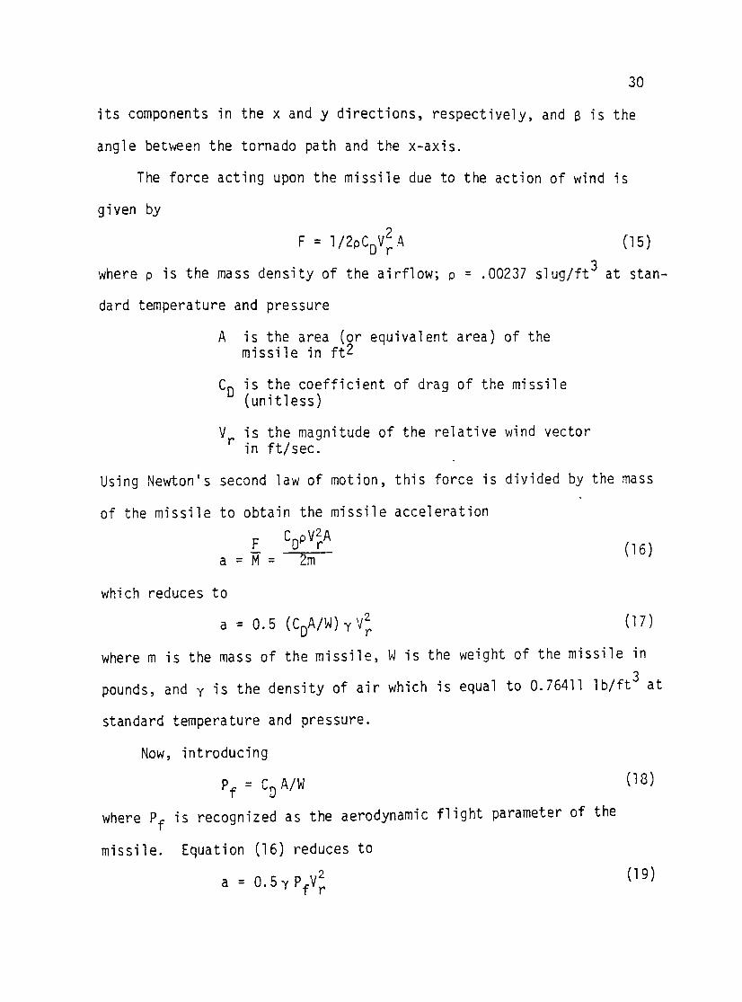
The drag force F that acts on the missile due to the resultant
wind vector is given by
where
( l )
p is the mass density of air
c0
is a drag coefficient that is a function of the missile shape, surface roughness and Reynolds number (in some cases)
V is the net resultant wind velocity vector
A is the area (or equivalent area) of the missile exposed to the wind vector
The missile acceleration due to the force of the wind is
F -a = m
where
m is the mass of the missile
y is pg, the unit weight of air
W is the missile weight
10
Thus, one measure of the missile acceleration is the so-called missile
flight parameter c0A;W.
If a body (missile) is streamlined and if no flow separation
occurs, it may behave like an airfoil, i.e. there is a lifting force
associated with horizontal flow. Most typical tornado missile shapes,
however, do not behave as an airfoil and thus are lifted only by the
vertical component of the wind field. None of the methodologies des
cribed in Table 1 consider the effect of a lift force.
An issue associated with the flight parameter that has sparked
considerable debate is the question of whether a missile rolls and
tumbles during flight along its trajectory, or whether it assumes some
invariant position relative to the resultant wind vector. The tumbling
or nontumbling issue affects the value of c0A used in the flight param
eter. Both the drag coefficient and the area could be different for
all objects, except spheres. In general, the methodologies have util
ized expressions for an equivalent area, which is supposed to account
for the effect of tumbling. All methods except Lee (1973) and
Bhattacharyya (1975) assume the tumbling mode. Each method uses a
different expression for equivalent area.
The missile weight does not appear to be a problem, if one is
considering the trajectory of a bare element such as a pipe, a beam,
11
or a pole. However, missiles generated by a real tornado are rarely
11 Clean, 11 but have other elements or pieces of deoris attached to them
for all or part of the missile flight. This situation affects values
c0, A, and W in an unmeasurable way. Thus, a more realistic and
manageable approach to trajectory calculation may be to consider
ranges of values of the flight parameter and not worry about individ
ual values of c0, A or W.
Initial Conditions
Bates and Swanson (_1967), in their original \'/Ork, discussed three
modes of tornado missile injection into the wind field: ramp, explos5va,
and aerodynamic lift. Ramp injection, according to their perception,
is possible when a missile first rolls or tumbles up an incline and
then becomes airborne. This injection mode is site dependent. The
explosive mode is associated with the effect of a rapid atmospheric
pressure change in a tornado. Recent research (Minor and Mehta, 1979)
discounts an explosive mode of failure due to atmospheric pressure
change for most ordinary buildings. Lee (1973) proposed an initial
impulse force that acted on the missile for a short period of time.
Associated with a coefficient of lift, the missile becomes airborne in
Lee's scheme if the lift force is sufficient to overcome the gravita
tional force of the object.
Most other approaches have simply placed the missile at some
arbitrary location relative to the tornado path and at some arbitrary
elevation above ground level. The tornadic winds are then allowed to
suddenly take effect. Parametric studies are performed to find the
12
location that produces the worst case relative to velocity achieved
and distance traveled by the missile. The missiles are released at
different elevations above ground, up to 200 ft. This approach is
taken because potential missiles could be located atop tall structures
during construction at a power plant site, and partly to give the
tornadic winds sufficient time to act on the missile before it impacts
with the ground.
Number of Degrees of Freedom
All methodologies except the one by Redmann, et al. (1978) consider
the missile as a point mass and treat the dynamic problem as one with
three degrees of freedom rather than six, which is the most general
case.
The diverse approaches to tornado missile trajectory calculations
and the diverse results obtained from these approaches suggest the need
to establish a rational approach based on the best and most logical
features of previous methodologies as well as new innovations.
Basis for Rational Approach
From review of previous work on missile trajectory calculations,
the following conclusions are reached regarding the various assumptions
required for a rational method of analysis:
1 )
2)
None of the wind field models used previously are sufficiently rigorous, have reasonable bounds, and yet are simple enough for engineering applications.
Possible variations of the elements of the aerodynamics flight parameters (c0, A and W) make it difficult to precisely define each one individually.
13
3) Missile injection into the wind field is not realistic and does not account for the anchorage forces resisting missile movement.
4) In light of our present knowledge of drag and lift coefficients for various types of missiles and the attachments they may have during flight, the three-degree-of-freedom dynamic model appears to be adequate for trajectory calculations.
5) None of the previously proposed methodologies have been used in an attempt to match missile behavior observed in an actual tornado.
The tornado missile trajectory model presented in this report
attempts to satisfy the requirements for a rational approach that is
consistent with technology as we presently know it.
Wind Field Model
Redmann, et al. (1976) provides an excellent critique of the
interpretation of Hoecker's analysis of the Dallas tornado. Attempts
to generalize the Dallas model for other tornadoes entails extrapolating
scaling relationships which have little or no physical basis. There is
no attempt to tie the results to basic fluid mechanic equations of
motion and continuity. Use of a combined Rankine vortex in lieu of the
Hoecker analysis for tangential wind variation is a justifiable simpli
fication. However, the models that use the combined Rankine vortex
have other deficiencies similar to those that use Hoecker's analysis.
The Kuo model is rigorous from a fluid dynamic point of view.
However, physical parameters required in the solution of the equations
are not easily defined. The model proposed by Redmann, et al. (1976)
has the rigor and the simplicity needed for engineering analysis. Un
necessary bounds on maximum wind speeds and an attempt to force the
14
model to satisfy (and justify) the so-called Tephigram method of bounds
on the potential intensity of a tornado renders the model less than
desirable for practical applications of missile trajectory calculations
for power plant licensing purposes.
The single vortex wind field model proposed by Fujita (1978) (as
opposed to his multiple vortex model) appears to satisfy most, if not
all, of the model defficiencies cited above; yet, it is simple enough
for engineering calculations. Designated DBT-77 (Design Basic Tornado
based on 1977 technology), the model is based on photogrammetric anal-
ysis of tornado movie films and on damage patterns observed in post-
storm investigations. Fluid mechanics equation of motion and continuity
are generally satisfied, and scaling parameters for adjusting the tor
nado size (radius of maximum wind speed) are consistent and have a
physical basis. The model is described in detail in Chapter III.
Aerodynamic Flight Parameter
Selection of the proper value for the aerodynamic flight param-
eter provides a series of contradictory problems.
1)
2)
3)
Missiles are rarely 11 Cl ean 11; they have attachments that affect
values of CD' A and W.
While a tumbling mode seems intuitively correct, there is evidence from tornado damage patterns that long slender missiles such as pipes, poles and beams tend to align themselves in the same direction.
The majority of long slender missiles impact 11 0n-end. 11 This position is inconsistent with the assumption that the maximum area of the missile aligns itself normal to the wind velocity vector.
These inconsistencies lead to the conclusion that precise values
of the aerodynamic flight parameter cannot be defined. Earlier attempts
15
to define equivalent area (Bates and Swanson, 1967; Beeth and Hobbs,
1975; Simiu and Cordes, 1976) are merely rationalization for reducing
the exposed area without any real physical basis (e.g. wind tunnel
tests). Therefore, the approach proposed herein is to consider reason
able ranges of values of flight parameters rather than attempts to
define specific values of c0, A and W. Upper bounds are obtained by
taking the largest values of c0 and A, but these may not be reasonable.
The effects of varying the flight parameter over a certain range is
illustrated in Chapter IV in association with the Bossier City tornado
missiles.
Initial Conditions
As defined, initial conditions apply to the conditions at the
missile prior to being affected by the tornaGo. The three initial
conditions are initial height, initial location relative to tornado
path, and missile release velocity Vmr· Observations of post-storm
damage indicate that objects lying loose on the ground or even at
some elevation above ground are rately (if ever) transported by the
wind. McDonald (1976) observed that utility poles that were stacked
on a rack five ft above ground were not transported by the Brandenburg,
Kentucky tornado of April 3, 1974. The poles were located in an ideal
position to be transported by one of the most intense tornadoes that
has ever occurred in the United States. Stacks of pipes, electrical
transformers and other types of loose objects were also not picked up.
Thus, it appears that some type of sudden release of an object is
16
required for it to be injected into the wind field. Such a release can
occur due to the sudden failure of connections or anchorages, by roof
uplift or wall collapse. Sudden release of the resisting forces pro
vided by anchors has the effect of an instantaneously applied force.
This force then accelerates the missile and moves it into position to
be affected by the drag force components of the wind.
In the trajectory model proposed herein, each missile type has an
associated missile release velocity V , which is the wind speed mr required to overcome the anchorage forces that resist movement of the
missile by the tornadic winds. The missile release velocity has a
significant effect on the path taken by the missile.
the missile may not be transported at all.
I f V i s sma 11 , mr
Since most missile shapes are not airfoils, the only uplift is
due to the vertical component of the wind field. A missile lying on
the ground will never be picked up if the vertical wind component is
zero at ground level, as it should be. A ramp-type injection as
perceived by Bates and Swanson (1967) is possible, if the missile
rolls and tumbles up a ramp and is lifted above the zero ground datum.
The above statements are consistent with observations of post-storm
damage. In the Brandenburg tornado, the winds blew past high stacks
of lumber. The. top boards were blown off of the stacks and some were
transported more than two miles. However, as the height of the stacks
decreased, they finally reached a level where no more boards ~Ere
picked up, indicating that when the stacks reached a certain level, the
vertical component of the wind was not able to sustain them in the wind
field.
17
The initial location of the missile relative to the tornado path
has two effects. If the missile is too far removed from the path, the
missile release velocity Vmr will never be reached, and the missile
will not be transported. The location of the missile relative to the
tornado path at Vmr also affects the path taken by the missile.
Number of Degrees of Freedom
While the six-degree-of-freedom approach taken by Redmann, et al.
(1978) is the most rigorous (it's hard to imagine a 12-in. dia pipe,
16ft long as a point mass), the variation of drag and lift coeffi-
cients as a function of missile attitude are not known. In the Redmann,
et al. study, a limited number of objects (12-in. dia pipe and auto
mobile) were tested full scale in a wind tunnel to obtain data on the
variation of the drag and lift coefficients. When the results of the
three-degree-of-freedom model and the six-degree-of-freedom model were
compared, they were not terribly different, although the six-degree-of
freedom model predicts slightly lower missile velocities.
Summary of Desired Trajectory Model Features
Based on review of previous attempts at tornado-generated missile
trajectory calculations, the following are judged to be the most
desirable features of a trajectory model:
1 )
2)
3)
Wind field model: DBT-77 by Fujita
Aerodynamic flight parameter: Use a range of values rather than specific values of CD, A and W.
Dynamic Model: Three degrees of freedom with a step-by-step numerical integration scheme.
4) Initial Conditions: Consider initial height above ground, initial location of missile relative to tornado path, and missile release velocity.
These features are described in detail in the next chapter.
18
III. MISSILE TRAJECTORY MODEL
The methodology, including the assumptions and the calculation
procedures, is referred to as the missile trajectory model. If cer
tain initial conditions about the tornado and the missile are speci
fied, the model gives information about the accelerations, the
velocities, and the displacements of the missile as a function of time.
The characteristics of the wind field model can also be changed as a
function of time.
Details of the trajectory model, along with assumptions and cal
culation procedures, are described in this chapter.
Wind Field Model
The assumptions and limitations on wind field models used previ
ously are discussed in Chapter II. The model that seems to best satis
fy requirements of rigor and simplicity is the single vortex model
proposed by Fujita (1978). This model, designated as DBT-77*, was
developed by Fujita as a design basis tornado in 1977 for use by engi
neers in the design and evaluation of structures. The model was
developed from the many observations of tornado damage and from photo
grammetric analysis of tornado movies. The wind field model satisfies
the basic laws of fluid dynamics, including continuity of flow.
*For fur the r i n format i on on 0 B T- 7 7 , see F u j i t a (J 9 7 8 ) ~
19
20
A schematic diagram of the single vortex wind model, DBT-77, is
shown in Figure l. The model is an axis-symmetrical vortex with a
cylindrical core. The core is divided into two parts: an inner core
with rad~us Rn, and an outer core with radius R0
. Vertical motions are
confined to the outer core. The inner core contains a region of rota
tional flow surrounded by the outer core which contains irrotational
flow.
The inflow layer has a height H., where air feeds into the outer l
core of the tornado and then flows vertically upward. Above the inflow
layer, the flow is outward.
The tangential velocity component in this model is expressed as the
product of two functions, each of which varies with height and radius.
The tangential velocity is given by
V = Flr) F(h) Vm (3)
where Vm is the maximum tangential wind speed; F(r) and F(h) are identi
fied as radial and height functions, respectively. They are given by
F ( r) =
~~~~ ~ F(h) =
r 1/r hko e-k(h-1)
( r < 1 )
~h: n (4)
(h > l)
where rand hare the normalized radius and the normalized height, res-
pectively, at which the tangential wind speed is calcualted. Values of
k0
and k are assumed to be l/6 and 0.03 in this model. Fujita (1978)
states that as more observational data are accumulated in the future,
the values of k0
and k may change slightly.
MAXIML'M TANGENTIAL VELOCITY, Vm~
I I
I ,; ~·· if.·'.; .· +t.:
I
I I
I I
I I
I
;.-INNER i COREJ OUTFLOW
J ' 1 '
----.. J ____ _ ~ )
OUTER CeRE
21
FIGURE l. SCHEMATIC DIAGRAM OF SINGLE VORTEX TORNADO MODEL- DBT-77
22
The radial wind speed is expressed in this model by
U = V tan a (5)
where a is the crossing angle, which denotes the angle between the
direction of the incoming air flow and a concentric circle of radius r
at their crossover point (See Figure 2). In this model, a is assumed
to be zero inside the inner core. It increases or decreases outward
within the outer core, reaching a0
at its outer edge. Outside the
core, a0
remains constant everywhere. The value of a is expressed by 0
= -A (1-h312) m
= B (1-e-k(h-1)) m
inside inflow layer (6)
outside inflow layer
where Am and Bm are positive nondimensional quantities called the
11 maximum inflow tangent 11 and the 11 maximum outflow tangent,11 respectively.
The vertical velocity component inside the inner core and outside
the outer core is assumed to be zero. Inside the outer core, the ver-
tical velocity is assumed to be horizontally uniform and may be expressed
by
w = w v o m where w is the normalized vertical velocity expressed by
0
w0
= 0.398[2e-k(h-l)]
(7)
(8)
In summary, the DBT-77 tornado wind field is completely defined if
three parameters are specified: Vm, R0
and Vt (the translational speed
of the tornado). The three components of wind velocity can be normalized
with respect to Vm. The normalized wind speeds are
u = U/V o m v0 = V/Vm w0 = W/Vm
(9)
0 < R < Rn
Rr'l < R < R0
R0 < R
Qt..= 0
0 < o<. ( =<.0
<><.-~ - 0
~ I '
( 0( =-o )
/ /
FIGURE 2. DEFINITION OF CROSSING ANGLE
23
At inflow heights (where h < 1)
uo = -A hl/6(1-h3/2) m
vo = hl/6
wo = 3/28 EA (16h7/ 6 - 7h8/ 3) m
where E = 0.55 and A = 0.75 are used in this model. m
At outflow heights (where h > 1)
where k1 = k(h-1 ).
u0
= 27/28 k ~ (e-kl - e-2ki)
vo = e-kl
w 0
= 2 7 I 2 8 E Am ( 2 e- k 1 - e-2 k 1 )
At the top of the inflow layer (where h = 1)
u = 0 0
vo = 1
w0
= 27/28 E Am
24
( 1 0)
( 11)
( 12)
The values of Vm' R0
and Vt can be varied with time, if appropriate.
With these three quantities defined at any time t, the three wind field
components, u , v , and w0
can be defined for any point in space. 0 0
Missile Characteristics
Whenever an object is placed in a moving fluid (or moves through a
stationary fluid, as is the case with misssiles), it will experience a
force in the direction of motion of the fluid relative to the object
(drag force) and it may experience a force normal to the flow direction
(lift force). Drag and lift forces are caused by the sum of the tangen
tial and normal forces at the surface of a body. Drag due to tangential
stresses is called friction or viscous drag. Drag due to normal
stresses is called pressure drag. It is usually dominant on bluff
bodies. Drag coefficients must be experimentally determined, and
they generally depend on Reynolds number. Drag coefficients of
shapes typical of tornado-generated missiles are summarized in
Hughes and Brighton (1967). Drag coefficients for additional
shapes, including the wide flange beam section, are given in
Heorner (1958).
If the missile traveled in a fixed attitude, then the area
normal to the flow, or the projected area, would be the appropriate
value to use in the drag force equation. However, because of the
questions relating to whether a missile tumbles or not, there is
25
no precise expression for area available. The ma~imum area gives an
upper bound value and is conservative but is not necessarily realis
tic. Not only does the area change from one side of the missile to
the other, but the drag coefficient may also change, as illustrated
in Figure 3.
If there are appendages or attachments to the missile during
flight, these also change the value of area. In a similar manner,
they also increase the weight, as well as the coefficient of drag,
of the missile.
Thus, because of the unknown factors in the c0, A and W terms
of the flight parameter, the trajectory model is set up to deal with
OB
JE
CT
F
AC
E
OP
PO
SIT
E
TO
C
OE
FF
ICIE
NT
O
F W
INO
V
EC
TO
R
DR
AG
A
HE
A
C0
A
HO
LL
OW
~---
11/
. I
2
HE
MIS
Plt
ER
E
d 0
.34
-
0.3
4 (
~
)
"'----
4 4
-------
-----------
--
-
HO
LL
OW
---)
2 .
2
HE
MIS
PH
ER
E
d 1
.42
11
d
14
2 (~)
4 .
4
-. t--·--
I-~l
WID
E
FL
AN
GE
)
SE
CT
ION
2
.0
(h}(
L)
2 (
h H
L)
i-----------
--------~----------
---~---
-------------~-
--
h t
--------t
W
IDE
F
LA
NG
E
)
~ [}
S
EC
TIO
N
1.0
(b)(
L)
I (b
)(L
)
FIGU
RE
3.
VARI
ATIO
N OF
DRA
G CO
EFFI
CIEN
T W
ITH
ORIE
NTAT
ION
OF M
ISSI
LE
! I I
N
0'\
27
one value of flight parameter rather than considering individual values
of all three parameters. It is necessary then to determine what range
of values the flight parameter can assume using reasonable variations
of c0, A and w. Initial Conditions
Three initial conditions affect the missile trajectory:
l) initial height above ground,
2) missile release velocity, and
3) location of missile relative to tornado path.
The trajectory model can handle a wide range of values for the three
parameters. The initial height above ground affects the value of the
vertical wind component which produces the only upward acting force on
the missile. Typical missile shapes are not airfoils and thus there
is no lift force, per se. The missile release velocity greatly affects
the path taken by the missile and determines to some extent if the mis
sile will move at all. If the missile release velocity is greater than
the wind speed that occurs at the missile location, the missile remains
stationary. If the release velocity is small, the missile does not
experience a large initial acceleration and may not travel very far.
The missile release velocity can be calculated if its anchorage strength
is known or can be estimated (Mehta, et al., 1976). Because of uncer
tainties of material strength, a range of V may have to be considered. mr The trajectory model assumes that the missile is at some fixed
location and the tornado translates past the missile. When the tornadic
28
wind speed at the missile location exceeds V , the missile begins to mr move. Otherwise, it remains stationary.
Appropriate values for initial missile height, V and initial mr location must be chosen consistent with conditions at the site in
question.
Equations of Motion
The equations of motion used in this study are based on a rectan-
gular coordinate system. The three wind components U, V, and t~ (the
radial, the tangential, and the vertical wind speed, respectively) are
converted to rectangular coordinates by the following transformation
equations:
v = X
u cos e- v sine
vy = u sine+ v cos e ( 13)
vz = w
where Vx and VY are the horizontal wind speeds in the x and y direc~ons,
respectively. V2
is the vertical wind speed in the z direction, and e
is the angle that the line joining the tornado center and the missile
position makes with the x-axis (See Fig. 4).
The translational wind speed is resolved into an x component and a
y component and added vectorially to Vx and Vy, respectively
vt = vt cos s X
vt = vt sin s y
( 14)
where vt is the translational velocity of the tornado, vtx and vtyare
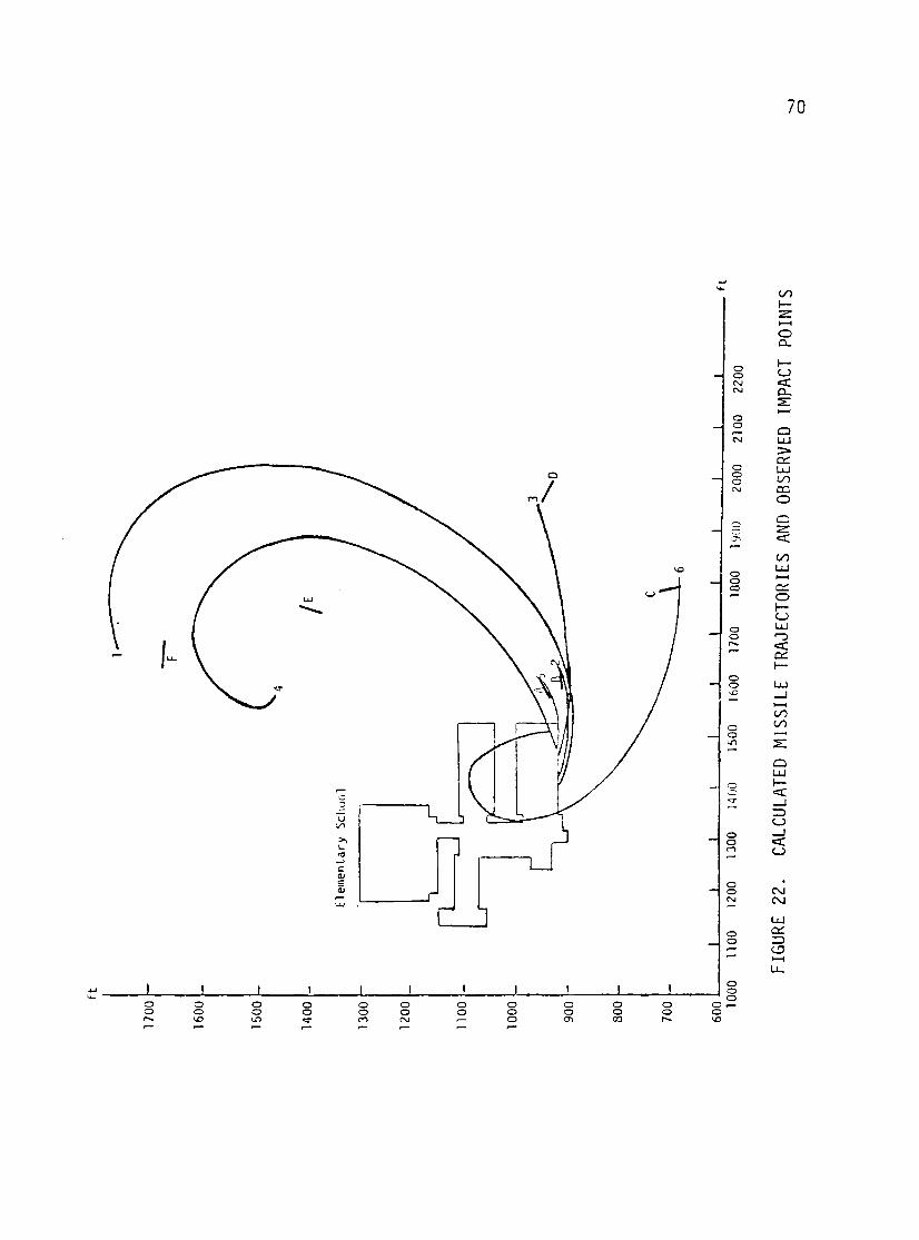
individual missile was selected and tabulated in Table 8. The trajec
tories are referred to as trajectories 1 to 6. The observed impact
points are labeled A to F. The coordinates of the observed impact
points and the calculated impact points and the errors are listed in
the table. Except for impact point E, the calculated points are
remarkably close. Figure 22 shows a horizontal olot of the 6 trajec
tories and the locations of the impact points.
Conclusions Based in Simulation Studies
Upon examination of values of missile release velocity and flight
parameters that were required to match the observed locations of all
six missiles, the following is observed:
1) The missile release velocities are relatively lovJ, compared to the calculated "ideal" release velocity of 170 mph.
2) Three of the six missiles required flight parameters that are near the lower limit of the acceptable range, and the other three required flight parameters that are near the upper limit.
3) While the impact points of the missiles match very well, the observed angles of impact do not match the calculated ones very well.
The justification of the low release velocities that were required
to match the observed impact location is that the tornadic winds might
have lifted parts of the roofing material prior to the release of the
missiles from their anchorage. This might have reduced the resistance
of the column release R, and hence the release velocity, Vmr
Because the beams were located along the top of the 140 ft wall,
they are not expected to have the same·values of flight parameter and
pf
v T
raje
ctor
y m
r N
umbe
r (f
Ulb
) (m
ph}
1 .2
60
95
2 .0
35
100
3 . 0
30
150
4 .2
80
100
5 .0
33
100
6 . 2
00
105
TABL
E 8
COM
PARI
SON
OF O
BSER
VED
AND
CALC
ULAT
ED
IMPA
CT L
OCAT
IONS
Max
. H
oriz
. M
ax.
Ver
t.
Max
imum
-O
bser
ved
-ta 1
cul a
ted
Ve1
ocit
) V
eloc
ity
Hei
ght
Imna
ct
Impa
ct
(fti
_sec
..
( ft/
sec)
_
(ft)
x(
f_tl
· y
( ft)
~{
ft)
y(f
t)
231
82
238
1450
17
10
1468
17
67
108
35
24
1410
91
5 14
11
916
145
45
54
1780
94
0 17
40
972
204
82
361
1535
14
00
1310
14
55
71
33
18
1375
94
5 13
85
944
144
61
189
1590
70
0 15
96
694
Mis
sile
M
atch
ed
F
B c E
A
D
Err
or
{ft
)
60 1 51
232 10
8
0'\
lO
ft
1700
1600
,_
1500
1400
·-
/E
Ele
men
tary
S
cho
ol
1300
1200
·-
1100
·-
1000
900
·-
300
700
·-~6
600
ft
1000
JJ
OO
12
00
JJO
Q
]4Q
Q
•rn
n
•·--
FIGU
RE
22.
CALC
ULAT
ED M
ISSI
LE T
RAJE
CTOR
IES
AND
OBSE
RVED
IM
PACT
PO
INTS
.....
._. 0
71
release velocity. Each would have more or less amounts of roof attached
and the anchorage failure resistance would be slightly variable.
The flight parameters required to match the observed impact loca
tions are all within the reasonable range defined earlier. The ~issiles
that did not travel very far (missiles A, B and D) are the ones that
required low flight parameters. Those that traveled long distances
(missiles C, E and F) are the ones that required high flight parameters.
A comparison between the observed and the calculated angles of
impact is shown in Table 9. Only three of the trajectories (trajec
tories l, 2 and 5) gave a very close match of the observed angles. Also
shown in Table 9 are the calculated impact velocities of the missiles.
Unfortunately, soil samples were not taken at the time of the tornado,
so the physical properties of the soil are not known. However, the
calculated impact velocities shown in the table suggest that the impacts
observed are feasible.
Missile
A
B
c
D
E
F
TABLE 9
COMPARISON OF OBSERVED AND CALCULATED IMPACT ANGLES
Observed Calculated ImQact Angle ImQact Angle
Horizontal Vertical Horizontal Vert1cal
N 50° E Unknown N 60° E 15°
N 85° E 30° N 85° E 15°
s 30° E Z3° N 70° E zoo
s 60° E 20° s 70° E 16°
N zoo w so s 80° E 4Z 0
N 85° W Unknown s 60° w 43°
7Z
Calculated Impact
Velocity
11 3 ft/ sec
79 ft/sec
150 ft/sec
153 ft/sec
7Z ft/sec
61 ft/sec
V. SUMMARY AND CONCLUSIONS
Summary
In this study, a rational approach for the simulation of tornado
generated missile trajectories has been presented. A wind field model
that is practical and has a physical basis is utilized in the formula
tion of a three-degree-of-freedom trajectory model that is realistic
and practical from an engineering point of view. The trajectory model
calculates the position, velocity, and acceleration of the missile as
functions of time. The model is capable of handling tornadoes with
parameters that vary with time. These parameters include the path,
the maximum tangential wind speed, the outer core radius, and the trans
lationa1 speed of the tornado.
The missile characteristics required for the trajectory simulation
are the initial conditions, the release velocity, and the flight param
eter. The initial conditions include the initial elevation and the
location of the missile relative to the tornado path. The release
velocity depends on the anchorage of the object to the structure and
the resistance of the structure to the wind-induced pressure. The
flight parameter can be calculated as a function of the drag coefficient,
area and weight of the missile. It can be accurately calculated for
bare missiles, but in the case where the missile has appendages or
attachments of unknown weight and area, the flight parameter varies
within a certain range and cannot be assigned a specific value.
73
74
Conclusions
The following conclusions on the trajectory simulation model and
the comparison of calculated missile behavior with observed missile
behavior are made:
1. A missile is sustained by the tornadic winds if a sudden
release is applied on it. As the missile release velocity
increases, the initial acceleration of the missile due to
the tornadic winds increases; hence, the missile travels
faster, higher, and further than one released at low wind
speeds.
2. Since mis-sfles are rarely "clean, 11 a range for the flight
parameter, rather than specific values of the coefficient of
drag, the area and the weight, is suggested.
3. The calculated impact locations of the six wide flange beam
missiles transported by the Bossier City tornado match very
closely with the observed ones; the calculated angles of
impact do not match the observed angles as well; and the
impact velocities resulting from the simulation are of
sufficient magnitude to cause the missiles to penetrate the
ground as observed.
LIST OF REFERENCES
Bates, F.C., and Swanson, A. E., ~lovember, 1967. 11 Tornado Design Consideration for ~iuclear Pov.1er Plants," The American Nuc~ear Society, ~nnual Meeting, Chicago, Illinois.
Beeth, D.R., and Hobbs, S.H., October, 1975. ''Analysis of Tornado-Generated Missiles," Topical Keport S&R-001.
Bhattacharyya, A.:<., 3oritz, R.C., and ~liyogi, P.K., October, 1975. ''Characteristics of Tornado-Generated Missiles," United '::ngineers, Inc., Philadelphia, Pennsylvania.
Fujita, T.T., September, 1978. "Workbook of Tornadoes and High Winds for Engineer-ing .:1.pplications," University of Chicago, S~!RP Research Paper 165, Chicago, Illinois.
Fujita, T.T., January, 1979. "Preliminary Report of the Bossier City Tornado of December 3, 1978," Department of Geophysical Sciences, University of Chicago, Chicago, Illinois.
Hoecker, W.H., Jr., Hay, 1960. "J.Jind Speed and ,-\ir Flow Patterns in the Jallas Tornado of .1\pril 2,"1957 ," Monthly '1Jeather Revie•.-J, Vol. 88, :lo. 5, pp. 167-180.
Heorner, S.F., 1965. "Fluid Dynamic Drag," Hoerner Fluid Dyna:nics, Sri ck T m~m, New Jersey.
Hughs, ~i.F., and Brighton, J.A., 1967. "Theory and Problems of :=luid Dynamics," Scham' s Outline Series, McGraw-Hill Book Compc.ny.
Iotti, R.C., June, 1975. "Design Basis Velocities of Tornado Genen~ed Missiles," Paper Presented at Annual Conference of American Nuclear Society, New Orleans, Louisiana.
James, R.A., Burdette, E.G., and Sun, C., November, 1974. "The Generation of Missiles by Tornadoes, 11 Tennessee Valley Authority, TVA- TR74-l.
Johnson, T., and Abbot, G., November, 1977. "Simulation of Tornado Missile Hazards to the Pilorim 2 Nuclear Thermal Generating Station,'' Science ,0-,pplications, Inc., Bechtel Power Corp., San Francisco, California.
Kuo, H. L. , January, 1971. "Assymmetr~ c Fl m•:s in the Sound a ry Layer of a Maintained Vortex,'~ Journal of Atmosoheric Sciences, Vol. 28 No. 1.
75
76
Lee, A.J.H., December, 1973. "A Study of Tornado Generated Missiles," ASCE Specialty Conference on Structural Design of Nuclear Power Plant Facilities, Chicago, Illinois.
McDonald, J.R., June, 1976. "Tornado-Generated Missiles and Their Effects," Symposium on Tornadoes: Assessment of Knowledae and Implications for Man, Texas Tech University, Lubbock: Texas.
Mehta, K.C., Minor, J.E., and McDonald, J.R., September, 1976. "Windspeed Analyses of April 3-4, 1974 Tornadoes, 11 Journal of the Structural Division, ASCE, Vol. 102, No. ST9.
Meyer, B.L., and Morrow, W.M., June, 1975. "Tornado Missile Risk Model," Bechtel Power Corpo_ration, San Francisco, California.
Minor, J.E., and Mehta, K.C., November, 1979. "Wind Damage Observations and Implications," Journal of the Structural Division, ASCE, Vol. 105, No. STll.
NRC, 1975. "Missiles Generated by Natural Phenomena," U.S. Nuclear Regulatory Commission, Standard Review Plan, Revision 1, Office of Nuclear Reactor Regulation, Washington, D.C.
Paddleford, D. F., April, 1969. "Characteristics of Tornado Generated Missiles, Nuclear Energy System, Westinghouse Electric Corporation, WCAP-7897.
Redmann, G. H., Radbill, J.R,, Marte, J.E., Dergarabedian, P., and Fendell, F.E., February, 1976. "Wind Field and Trajectory Mode 1 s for Tornado Prope 11 ed Objects,'' El ectri ca 1 Power Research Institute, Technical Report l, Palo Alto, California.
Simiu, E., and Cordes, M., April, 1976. 11 Tornado Borne ~1issile Speeds," Institute for Basic Standards, National Bureau of Standards, prepared for the U.S. NRC, Washington, D.C.