Page 1
8/9/2019 Simulation of Whistle Noise Using Computational Fluid Dynamics
http://slidepdf.com/reader/full/simulation-of-whistle-noise-using-computational-fluid-dynamics 1/127
University of Kentucky
UKnowledge
eses and Dissertations--Mechanical Engineering Mechanical Engineering
2012
SIMULATION OF WHISTLE NOISE USINGCOMPUTATIONAL FLUID DYNAMICS
AND ACOUSTIC FINITE ELEMENTSIMULATION
Jiawei LiuUniversity of Kentucky , [email protected]
is Master's esis is brought to you for free and open access by the Mechanical Engineering at UKnowledge. It has been accepted for inclusion in
eses and Dissertations--Mechanical Engineering by an authorized administrator of UKnowledge. For more information, please contact
[email protected] .
Recommended CitationLiu, Jiawei, "SIMULATION OF WHISTLE NOISE USING COMPUTATIONAL FLUID DYNAMICS AND ACOUSTIC FINITEELEMENT SIMULATION" (2012). Teses and Dissertations--Mechanical Engineering. Paper 9.hp://uknowledge.uky.edu/me_etds/9
Page 2
8/9/2019 Simulation of Whistle Noise Using Computational Fluid Dynamics
http://slidepdf.com/reader/full/simulation-of-whistle-noise-using-computational-fluid-dynamics 2/127
STUDENT AGREEMENT:
I represent that my thesis or dissertation and abstract are my original work. Proper aribution has beengiven to all outside sources. I understand that I am solely responsible for obtaining any needed copyrightpermissions. I have obtained and aached hereto needed wrien permission statements(s) from the
owner(s) of each third-party copyrighted maer to be included in my work, allowing electronicdistribution (if such use is not permied by the fair use doctrine).
I hereby grant to e University of Kentucky and its agents the non-exclusive license to archive and makeaccessible my work in whole or in part in all forms of media, now or hereaer known. I agree that thedocument mentioned above may be made available immediately for worldwide access unless apreapproved embargo applies.
I retain all other ownership rights to the copyright of my work. I also retain the right to use in future works (such as articles or books) all or part of my work. I understand that I am free to register thecopyright to my work.
REVIEW, APPROVAL AND ACCEPTANCE
e document mentioned above has been reviewed and accepted by the student’s advisor, on behalf of the advisory commiee, and by the Director of Graduate Studies (DGS), on behalf of the program; we
verify that this is the nal, approved version of the student’s dissertation including all changes required by the advisory commiee. e undersigned agree to abide by the statements above.
Jiawei Liu, Student
Dr. David W. Herrin, Major Professor
Dr. J. M. McDonough, Director of Graduate Studies
Page 3
8/9/2019 Simulation of Whistle Noise Using Computational Fluid Dynamics
http://slidepdf.com/reader/full/simulation-of-whistle-noise-using-computational-fluid-dynamics 3/127
SIMULATION OF WHISTLE NOISE USING COMPUTATIONAL
FLUID DYNAMICS AND ACOUSTIC FINITE ELEMENT SIMULATION
THESIS
A thesis submitted in partial fulfillment of the
requirements for the degree of Master of Science
in Mechanical Engineering in the College of Engineering
at the University of Kentucky
By
Jiawei Liu
Lexington, Kentucky
Director: Dr. D. W. Herrin, Professor of Mechanical Engineering
Co-director: Dr. Tingwen Wu, Professor of Mechanical Engineering
Lexington, Kentucky
2012
Copyright © Jiawei Liu 2012
Page 4
8/9/2019 Simulation of Whistle Noise Using Computational Fluid Dynamics
http://slidepdf.com/reader/full/simulation-of-whistle-noise-using-computational-fluid-dynamics 4/127
ABSTRACT OF THESIS
SIMULATION OF WHISTLE NOISE USING COMPUTATIONAL
FLUID DYNAMICS AND ACOUSTIC FINITE ELEMENT SIMULATION
The prediction of sound generated from fluid flow has always been a difficult
subject due to the nonlinearities in the governing equations. However, flow noise can
now be simulated with the help of modern computation techniques and super computers.
The research presented in this thesis uses the computational fluid dynamics (CFD) and
the acoustic finite element method (FEM) in order to simulate the whistle noise caused by
vortex shedding. The acoustic results were compared to both analytical solutions and
experimental results to better understand the effects of turbulence models, fluid
compressibility, and wall boundary meshes on the acoustic frequency response. In thecase of the whistle, sound power and pressure levels are scaled since 2-D models are used
to model 3-D phenomenon. The methodology for scaling the results is detailed.
KEYWORDS: Acoustics, CFD, Whistle Noise, Finite Element Method, Scaling
Jiawei Liu
June 21, 2012
Page 5
8/9/2019 Simulation of Whistle Noise Using Computational Fluid Dynamics
http://slidepdf.com/reader/full/simulation-of-whistle-noise-using-computational-fluid-dynamics 5/127
SIMULATION OF WHISTLE NOISE USING COMPUTATIONAL
FLUID DYNAMICS AND ACOUSTIC FINITE ELEMENT SIMULATION
By
Jiawei Liu
Dr. D.W. Herrin
(Director of Thesis)
Dr. Tingwen Wu
(Co-director of Thesis)
Dr. J. M. McDonough
(Director of Graduate Studies)
June 21st , 2012
Page 6
8/9/2019 Simulation of Whistle Noise Using Computational Fluid Dynamics
http://slidepdf.com/reader/full/simulation-of-whistle-noise-using-computational-fluid-dynamics 6/127iii
ACKNOLEDGMENTS
I would like to express my sincere thankfulness to my graduate study advisor, Dr.
David W. Herrin, for his guidance and patience during my graduate study at the
University of Kentucky. I am also grateful to Dr. Herrin for giving me the opportunities
to participate in trainings and conferences and providing me with exposure to industrial
projects. I would also like to thank Dr. Tingwen Wu, the co-director of this thesis, for his
help and advice during both my undergraduate and graduate studies. My sincere
appreciation also goes to Dr. Sean Baily and Dr. James McDonough, who have provided
insights which guided and challenged my thinking, and substantially improving the thesis.
I am also grateful to the students and friends, Jinghao Liu, Xin Hua, Limin Zhou,
Srinivasan Ramalingam, Yitian Zhang and Rui He, who all have helped me and made my
stay full of fun memories.
And finally, thank you Mom and Dad for supporting me on everything.
Page 7
8/9/2019 Simulation of Whistle Noise Using Computational Fluid Dynamics
http://slidepdf.com/reader/full/simulation-of-whistle-noise-using-computational-fluid-dynamics 7/127iv
Table of Contents
ACKNOLEDGMENTS ................................................................................................... III
LIST OF TABLES ........................................................................................................ VIII
LIST OF FIGURES ........................................................................................................ IX
INTRODUCTION .................................................................................... 1 CHAPTER 1
1.1 INTRODUCTION ........................................................................................................ 1
1.2 OBJECTIVES ............................................................................................................. 3
1.3 MOTIVATION ........................................................................................................... 4
1.4 APPROACH AND JUSTIFICATION ................................................................................... 4
1.5 ORGANIZATION ........................................................................................................ 4
BACKGROUND...................................................................................... 6 CHAPTER 2
2.1 ACOUSTIC SOURCES .................................................................................................. 6
2.1.1 Monopole ........................................................................................................ 6
2.1.2 Dipole .............................................................................................................. 7
2.1.3 Quadrupoles .................................................................................................... 9
2.2 VORTEX SHEDDING ................................................................................................. 10
2.3 SOUND INDUCED BY VORTEX SHEDDING ...................................................................... 15
2.4 LIGHTHILL ANALOGY ............................................................................................... 18
2.4.1 Development of Lighthill’s Analogy .............................................................. 19
2.5 CFD TURBULENCE MODELS ...................................................................................... 23
Page 8
8/9/2019 Simulation of Whistle Noise Using Computational Fluid Dynamics
http://slidepdf.com/reader/full/simulation-of-whistle-noise-using-computational-fluid-dynamics 8/127v
2.5.1 Turbulence Model .............................................................................. 23
2.5.2 model ................................................................................................. 24
2.5.3 Large Eddy Simulation .................................................................................. 28
2.6 ACOUSTIC FEM ..................................................................................................... 30
2.6.1 Introduction ................................................................................................... 30
2.6.2 Infinite Element ............................................................................................. 32
SIMULATION APPROACH .................................................................... 35 CHAPTER 3
3.1 INTRODUCTION ...................................................................................................... 35
3.1.1 Computational Aeroacoustics ....................................................................... 35
3.1.2 CFD-Sound Propagation Solver Coupling ...................................................... 36
3.1.3 Broadband Noise Sources Models................................................................. 37
3.2 GENERAL ASSUMPTIONS .......................................................................................... 37
3.2.1 Model Dimension .......................................................................................... 37
3.2.2 Fluid Compressibility ..................................................................................... 38
3.2.3 Interactions and Feedbacks .......................................................................... 39
3.3 CFD-SOUND PROPAGATION SOLVER COUPLING PROCESS .............................................. 40
3.3.1 Comments on Source Mapping ..................................................................... 41
3.4 FAST FOURIER TRANSFORM FOR AEROACOUSTIC SIMULATION ........................................ 42
3.4.1 Determine Time Step Size and Number of Time Steps for CFD Simulation ... 42
3.5 WALL BOUNDARY MESHING REQUIREMENTS .............................................................. 43
3.6 SCALING OF ACOUSTIC RESULT .................................................................................. 45
3.6.1 Sound Power Scaling Laws ............................................................................ 45
Page 9
8/9/2019 Simulation of Whistle Noise Using Computational Fluid Dynamics
http://slidepdf.com/reader/full/simulation-of-whistle-noise-using-computational-fluid-dynamics 9/127vi
3.6.2 Finite Length Scaling ..................................................................................... 46
VERIFICATION OF SIMULATION APPROACH ........................................ 48 CHAPTER 4
4.1 LID-DRIVEN TEST CASE FOR MESH SELECTION ............................................................. 48
4.1.1 CFD Mesh Types ............................................................................................ 48
4.1.2 Lid-Driven Case Meshes ................................................................................ 50
4.1.3 CFD Simulation Setup .................................................................................... 51
4.1.4 Result and Discussion .................................................................................... 53
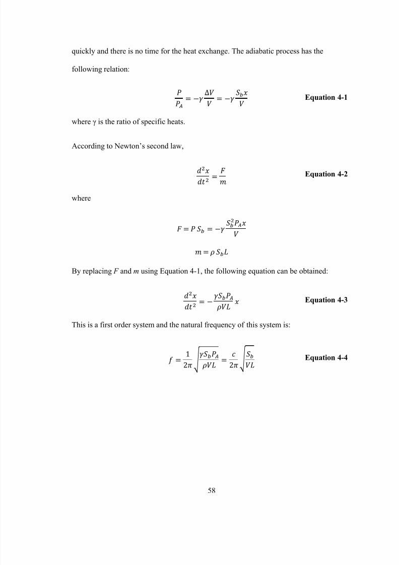
4.2 HELMHOLTZ RESONATOR CASE STUDY ....................................................................... 57
4.2.1 Helmholtz Resonator ..................................................................................... 57
4.2.2 Geometry and Mesh...................................................................................... 60
4.2.3 Simulation Setup and Steps........................................................................... 62
4.2.3.1 Steady State Solution ............................................................................ 64
4.2.3.2 Transient Solution ................................................................................. 66
4.2.3.3 Acoustic Solution .................................................................................. 69
4.2.4 Result and Discussion .................................................................................... 73
4.3 FLOW OVER CYLINDER CASE STUDY ........................................................................... 74
4.3.1 Geometry and Mesh...................................................................................... 75
4.3.2 Transient CFD solution .................................................................................. 78
4.3.3 Acoustic Simulation ....................................................................................... 81
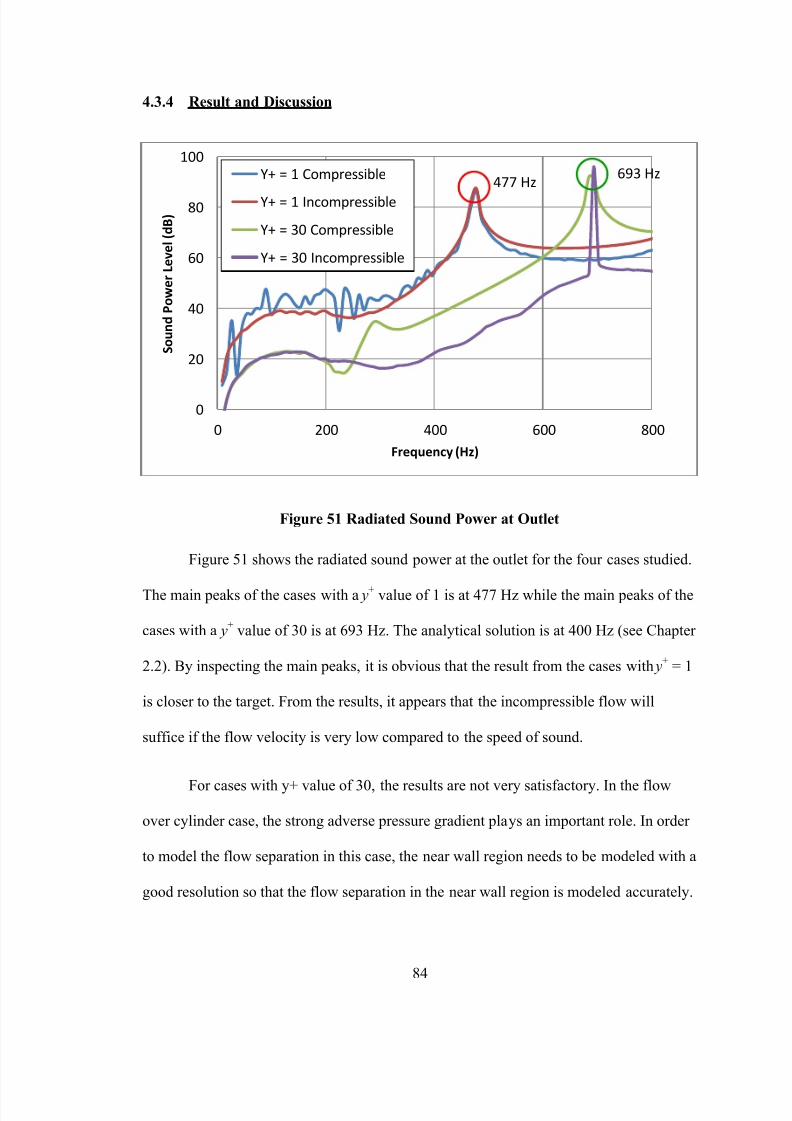
4.3.4 Result and Discussion .................................................................................... 84
WHISTLE CASE STUDY – MEASUREMENT AND SIMULATION ................ 86 CHAPTER 5
Page 10
8/9/2019 Simulation of Whistle Noise Using Computational Fluid Dynamics
http://slidepdf.com/reader/full/simulation-of-whistle-noise-using-computational-fluid-dynamics 10/127vii
5.1 WHISTLE GEOMETRY .............................................................................................. 86
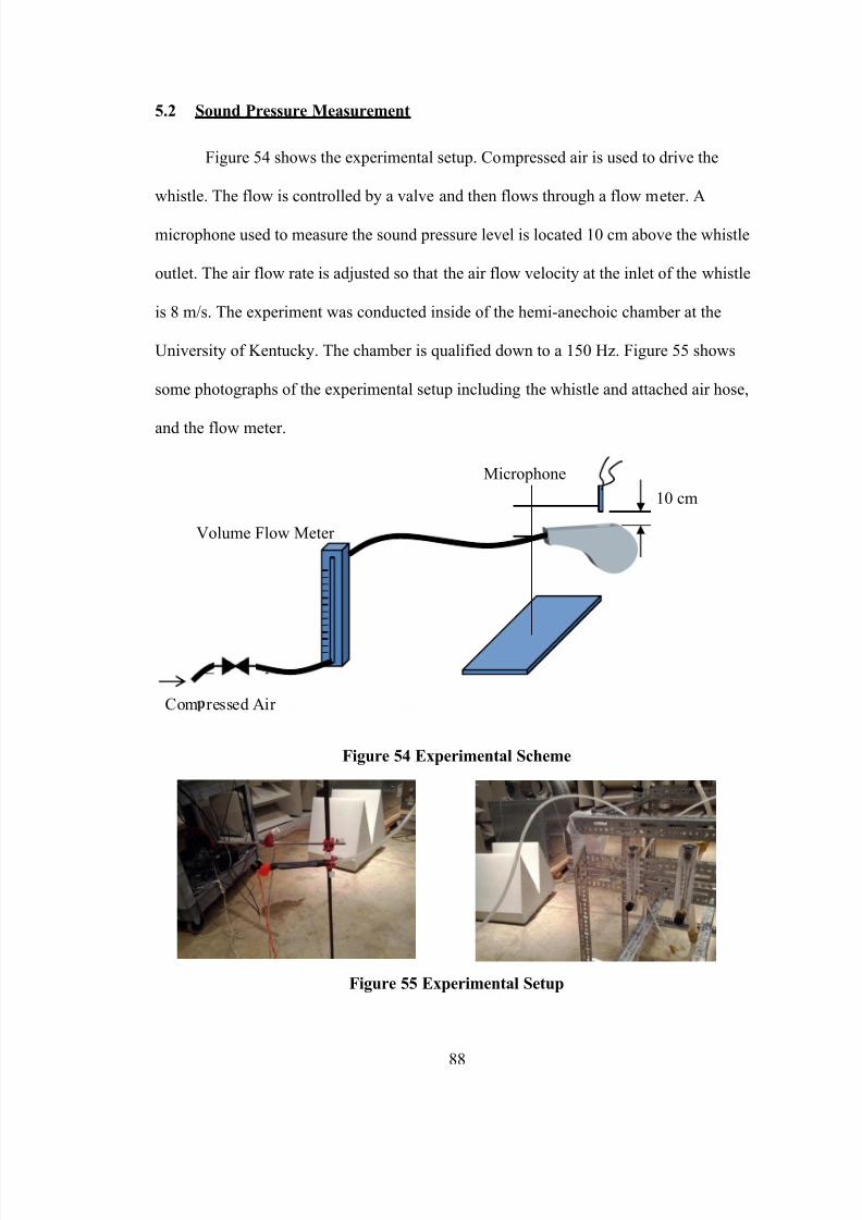
5.2 SOUND PRESSURE MEASUREMENT ............................................................................ 88
5.3 CFD SIMULATION .................................................................................................. 90
5.3.1 CFD Mesh ...................................................................................................... 90
5.3.2 CFD Simulations ............................................................................................ 91
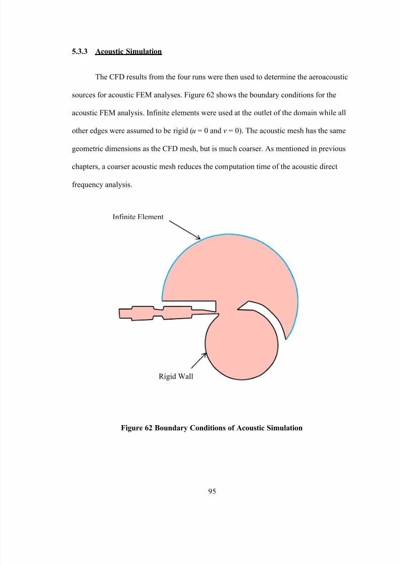
5.3.3 Acoustic Simulation ....................................................................................... 95
5.3.4 Scaling ........................................................................................................... 96
5.3.5 Results and Discussion .................................................................................. 97
SUMMARY AND FUTURE WORK ....................................................... 100 CHAPTER 6
6.1 SUMMARY .......................................................................................................... 100
6.2 FUTURE WORK .................................................................................................... 102
REFERENCES ........................................................................................................ 104
VITA .................................................................................................................... 113
Page 11
8/9/2019 Simulation of Whistle Noise Using Computational Fluid Dynamics
http://slidepdf.com/reader/full/simulation-of-whistle-noise-using-computational-fluid-dynamics 11/127viii
List of Tables
Table 1 Scaling Laws for Sound Power in Sound Fields with Different Dimensions ...... 46
Table 2 Dimension of the Simulated Helmholtz Resonator ............................................. 61
Table 3 Steady State Simulation Setup ............................................................................. 65
Table 4 Transient LES Simulation Setup.......................................................................... 66
Table 5 y+ and Corresponding Wall Height ...................................................................... 76
Table 6 Transient SST Simulation Setup ............................................................... 79
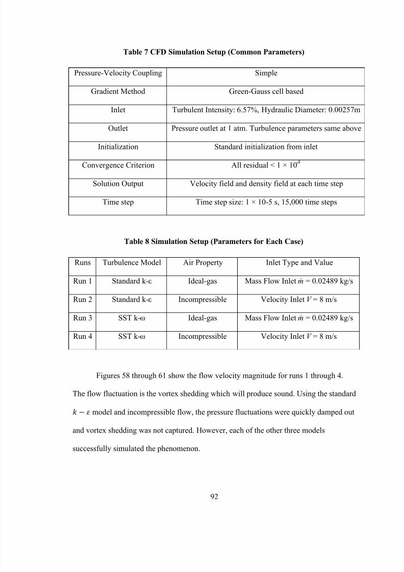
Table 7 CFD Simulation Setup (Common Parameters) .................................................... 92
Table 8 Simulation Setup (Parameters for Each Case) ..................................................... 92
Page 12
8/9/2019 Simulation of Whistle Noise Using Computational Fluid Dynamics
http://slidepdf.com/reader/full/simulation-of-whistle-noise-using-computational-fluid-dynamics 12/127ix
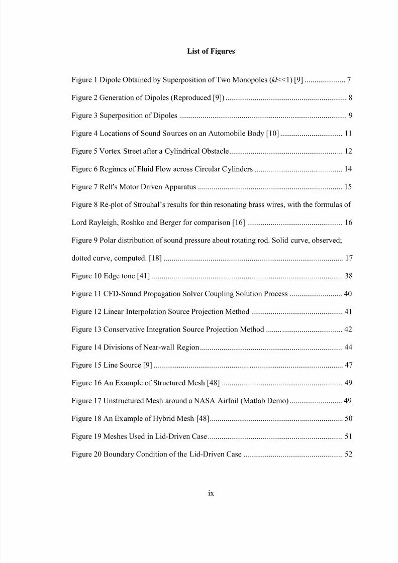
List of Figures
Figure 1 Dipole Obtained by Superposition of Two Monopoles (kl <<1) [9] ..................... 7
Figure 2 Generation of Dipoles (Reproduced [9]) .............................................................. 8
Figure 3 Superposition of Dipoles ...................................................................................... 9
Figure 4 Locations of Sound Sources on an Automobile Body [10] ................................ 11
Figure 5 Vortex Street after a Cylindrical Obstacle .......................................................... 12
Figure 6 Regimes of Fluid Flow across Circular Cylinders ............................................. 14
Figure 7 Relf's Motor Driven Apparatus .......................................................................... 15
Figure 8 Re- plot of Strouhal’s results for thin resonating brass wires, with the formulas of
Lord Rayleigh, Roshko and Berger for comparison [16] ................................................. 16
Figure 9 Polar distribution of sound pressure about rotating rod. Solid curve, observed;
dotted curve, computed. [18] ............................................................................................ 17
Figure 10 Edge tone [41] .................................................................................................. 38
Figure 11 CFD-Sound Propagation Solver Coupling Solution Process ........................... 40
Figure 12 Linear Interpolation Source Projection Method ............................................... 41
Figure 13 Conservative Integration Source Projection Method ....................................... 42
Figure 14 Divisions of Near-wall Region ......................................................................... 44
Figure 15 Line Source [9] ................................................................................................. 47
Figure 16 An Example of Structured Mesh [48] .............................................................. 49
Figure 17 Unstructured Mesh around a NASA Airfoil (Matlab Demo) ........................... 49
Figure 18 An Example of Hybrid Mesh [48] .................................................................... 50
Figure 19 Meshes Used in Lid-Driven Case ..................................................................... 51
Figure 20 Boundary Condition of the Lid-Driven Case ................................................... 52
Page 13
8/9/2019 Simulation of Whistle Noise Using Computational Fluid Dynamics
http://slidepdf.com/reader/full/simulation-of-whistle-noise-using-computational-fluid-dynamics 13/127x
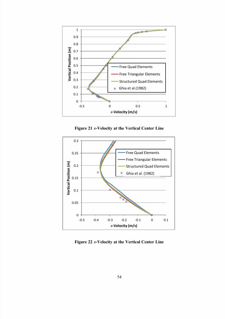
Figure 21 x-Velocity at the Vertical Center Line .............................................................. 54
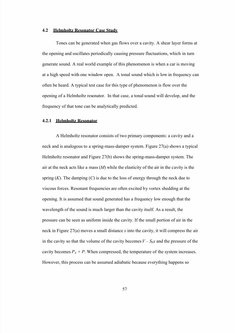
Figure 22 x-Velocity at the Vertical Center Line .............................................................. 54
Figure 23 Velocity Contour Plot (Free Quad Elements) .................................................. 55
Figure 24 Velocity Contour Plot (Structured Quad Elements) ......................................... 55
Figure 25 Continuity Residual History ............................................................................. 56
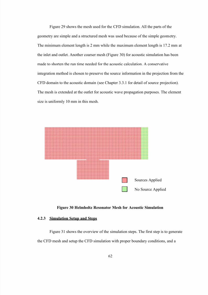
Figure 26 Friction Coefficient History (At the Moving Wall) ......................................... 56
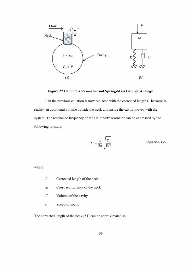
Figure 27 Helmholtz Resonator and Spring-Mass Damper Analogy ............................... 59
Figure 28 Geometry of the Simulated Helmholtz Resonator............................................ 60
Figure 29 Helmholtz Resonator Mesh for CFD Simulation ............................................. 61
Figure 30 Helmholtz Resonator Mesh for Acoustic Simulation ....................................... 62
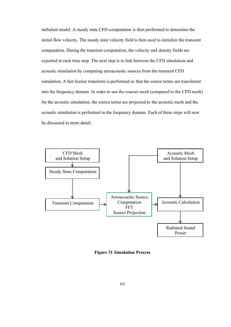
Figure 31 Simulation Process ........................................................................................... 63
Figure 32 Velocity Contour Plot (Steady State) ............................................................... 65
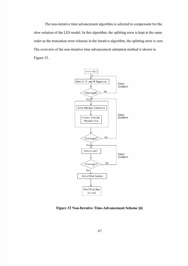
Figure 33 Non-Iterative Time-Advancement Scheme [6] ................................................ 67
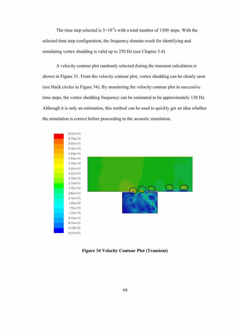
Figure 34 Velocity Contour Plot (Transient) .................................................................... 68
Figure 35 FFT with Integer Number of Periods ............................................................... 70
Figure 36 FFT with Non-Integer Number of Periods ....................................................... 70
Figure 37 FFT with Non-Integer Number of Periods (Windowed) .................................. 71
Figure 38 Divergence of Lighthill Surface at 131 Hz....................................................... 72
Figure 39 Direct Frequency Analysis Setup ..................................................................... 73
Figure 40 Radiated Sound Power at Outlet....................................................................... 73
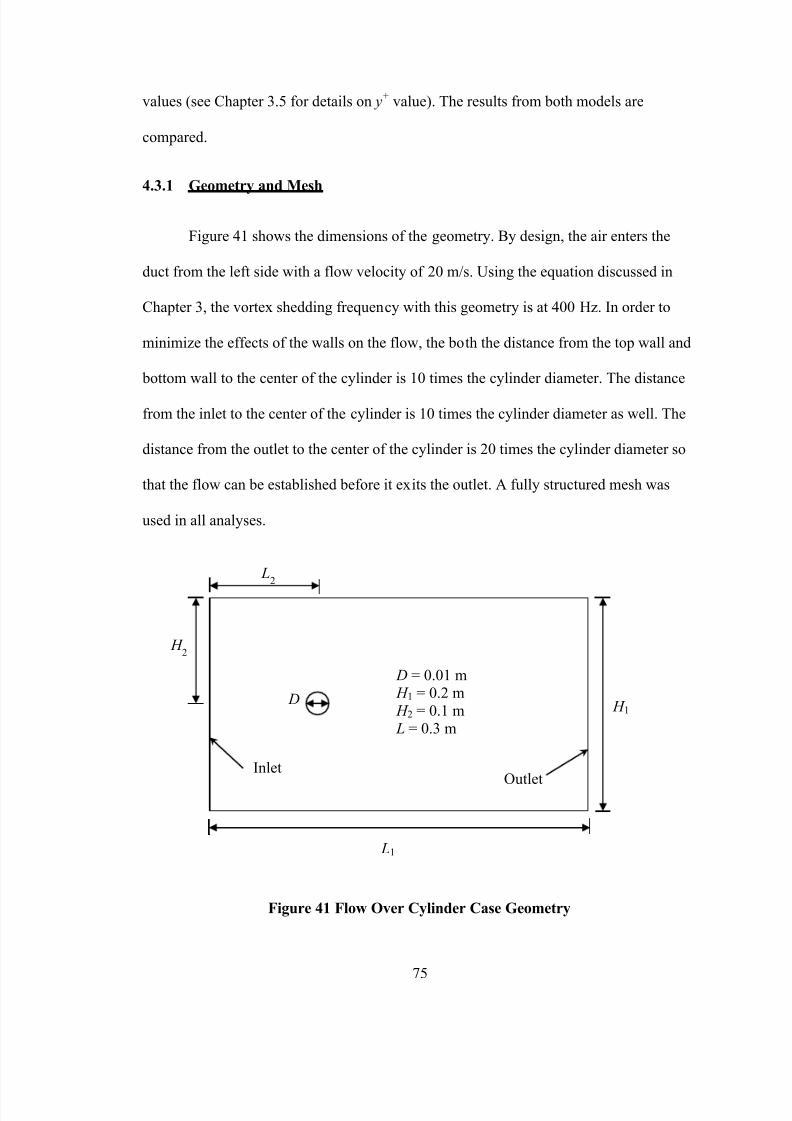
Figure 41 Flow Over Cylinder Case Geometry ................................................................ 75
Figure 42 Mesh for the Flow Over Cylinder Case ............................................................ 77
Figure 43 Acoustic Mesh for the Flow Over Cylinder Case ............................................ 77
Page 14
8/9/2019 Simulation of Whistle Noise Using Computational Fluid Dynamics
http://slidepdf.com/reader/full/simulation-of-whistle-noise-using-computational-fluid-dynamics 14/127xi
Figure 44 Velocity Contour of Compressible Flow, y+ = 1 Case ..................................... 79
Figure 45 Velocity Contour of Incompressible Flow, y+ = 1 Case ................................... 80
Figure 46 Velocity Contour of Compressible Flow, y+ = 30 Case ................................... 80
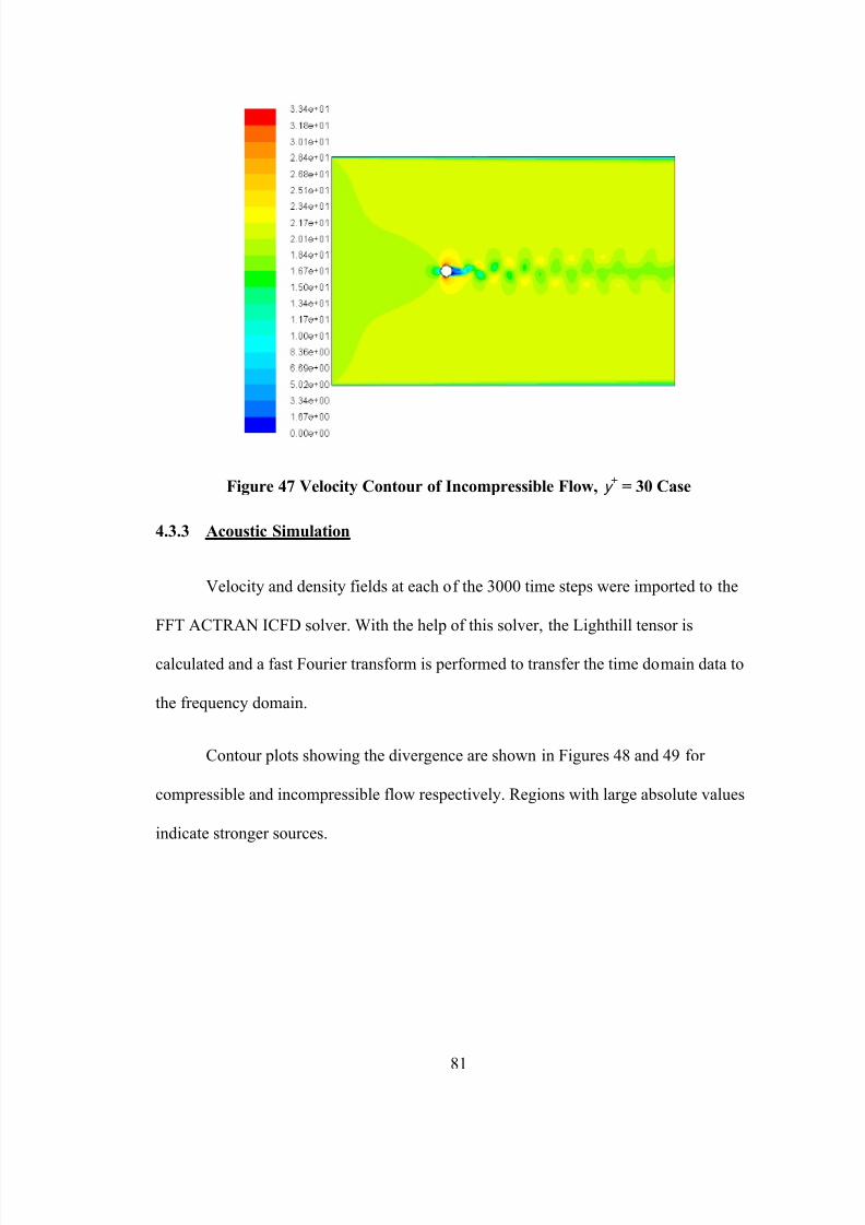
Figure 47 Velocity Contour of Incompressible Flow, y+ = 30 Case ................................. 81
Figure 48 Divergence of Lighthill Surface at 477 Hz (Compressible, y+ = 1) ................. 82
Figure 49 Divergence of Lighthill Surface at 477 Hz (Incompressible, y+ = 1) ............... 82
Figure 50 Direct Frequency Analysis Setup ..................................................................... 83
Figure 51 Radiated Sound Power at Outlet....................................................................... 84
Figure 52 Solid Model of the Whistle............................................................................... 87
Figure 53 Cross Section of the Whistle ............................................................................ 87
Figure 54 Experimental Scheme ....................................................................................... 88
Figure 55 Experimental Setup .......................................................................................... 88
Figure 56 Averaged Measured Sound Pressure Level ...................................................... 89
Figure 57 CFD Mesh of the Whistle ................................................................................. 91
Figure 58 Contour of Velocity Magnitude (Run1) ........................................................... 93
Figure 59 Contour of Velocity Magnitude (Run2) ........................................................... 93
Figure 60 Contour of Velocity Magnitude (Run3) ........................................................... 94
Figure 61 Contour of Velocity Magnitude (Run4) ........................................................... 94
Figure 62 Boundary Conditions of Acoustic Simulation .................................................. 95
Figure 63 Scale the Sound Pressure of a Whistle ............................................................. 97
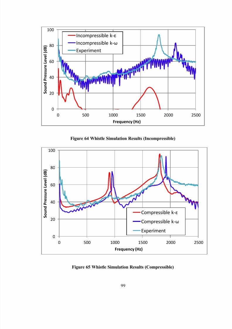
Figure 64 Whistle Simulation Results (Incompressible) .................................................. 99
Figure 65 Whistle Simulation Results (Compressible) ..................................................... 99
Page 15
8/9/2019 Simulation of Whistle Noise Using Computational Fluid Dynamics
http://slidepdf.com/reader/full/simulation-of-whistle-noise-using-computational-fluid-dynamics 15/127
1
Chapter 1
Introduction
1.1 Introduction
When talking about acoustics, most people relate it to music. However, music,
joyful sound, is not the only important aspect in acoustics. Acoustic noise is a major
concern of society and industry, and aerodynamic or flow noise is especially concerning
because it is closely related to the level of comfort of the environments in which people
live and work. Common examples of aerodynamic noise are jet noise and noise generated
when fluid flows over obstacles and cavities.
The prediction of sound generated from fluid flow has always been a difficult
subject due to the nonlinearities in the governing equations. However, flow noise can
now be simulated with the help of modern computation techniques and super computers.
Aerodynamic noise is a result of unsteady gas flow and the interaction of the
unsteady gas flow with the associated structure. The unwanted gas flow and structure
interaction may cause serious problems in industrial products such as the instability of the
structures and structure fatigue [1]. Accordingly, simulating the aerodynamic noise is
necessary and will improve the quality of the products at the design stage. However, due
to the nature of turbulent flow and the limitation of computational power, it is not always
feasible to obtain a reliable unsteady (transient) CFD solution for the aerodynamic noise
analysis. The computational effort and time is a major hindrance. Even if there were no
time limitation, any one of the commonly used turbulent models is not capable of solving
Page 16
8/9/2019 Simulation of Whistle Noise Using Computational Fluid Dynamics
http://slidepdf.com/reader/full/simulation-of-whistle-noise-using-computational-fluid-dynamics 16/127
2
all scales of turbulence. Therefore, a time-efficient method with acceptable accuracy is
needed in order to estimate flow noise.
Several well-known theories such as the theory of Lighthill [2] and the theory of
Ffowcs Williams and Hawkings (FWH) [3] have been successfully applied to
aeroacoustic problems. The theory of Lighthill is the foundation of the FWH approach. In
Lighthill’s paper, it has been shown that aerodynamic sound sources can be modeled as
series of monopoles, dipoles, and quadrupoles generated by the turbulence in an ideal
fluid region surrounded by a large fluid region at rest (i.e., velocity field in the fluid is
zero).
In Lighthill’s analogy, no fluid flow and sound wave interaction is considered. A
justification of this assumption has been given in Lighthill’s original paper . Due to the
large difference in energy, there is very little feedback from acoustics to the flow. For
flows in the low Mach number regimes, direct simulations are often costly, unstable,
inefficient and unreliable due to the presence of rapidly oscillating acoustic waves (with
periods proportional to the Mach number) in the equations themselves [4]. Even with the
aforementioned difficulties, reliable results are sometimes obtained using a combination
of incompressible (or compressible) flow solvers and Lighthill’s analogy at low Mach
number [5].
Commercial codes such as ANSYS FLUENT have incorporated the FWH
approach in a computational aeroacoustics module. FWH assumes that there are no
obstacles between the sound sources and the receivers [6]. Therefore, the sound radiation
problem is inherently a weak part of the simulation, especially if the sound source is in a
Page 17
8/9/2019 Simulation of Whistle Noise Using Computational Fluid Dynamics
http://slidepdf.com/reader/full/simulation-of-whistle-noise-using-computational-fluid-dynamics 17/127
3
waveguide or duct, enclosed, or obstructed in some way. One way to bypass this problem
is to utilize acoustic finite element simulation and use infinite elements to simulate
acoustic radiation at the boundary of the mesh.
This thesis examines the combination of the CFD solvers and the infinite element
technique for the prediction of sound radiated from turbulent flow with the effects of
vortex shedding. Based on the results derived from the test cases, guidelines for CFD
modeling of low subsonic flow noise caused by vortex shedding is documented in an
effort to improve the efficiency of the modeling process and select proper turbulent
models.
1.2 Objectives
This study will use the commercial code ANSYS FLUENT as a pure CFD solver
and FFT ACTRAN as the acoustic wave solver. The sound pressure or sound power
generated by turbulent flows will be obtained and compared to the theoretical values.
The cases studied include sound generated by:
a. Flow over a cylinder
b. Flow over a cavity (Helmholtz Resonator)
c. Flow in a sports whistle
The study will be restricted to 2-D models with vortex shedding frequencies expected to
be under or close to 2000 Hz. Fluid-structure interaction will not be considered in this
study. Though the cases studied do not completely reflect real world situations, the
Page 18
8/9/2019 Simulation of Whistle Noise Using Computational Fluid Dynamics
http://slidepdf.com/reader/full/simulation-of-whistle-noise-using-computational-fluid-dynamics 18/127
4
guidelines presented herein should benefit the simulation of future, more complicated
situations.
1.3 Motivation
Noise induced by flow over obstacles is a common engineering problem. In most
instances, vortex shedding is the major culprit. Of course, vortex induced vibration (VIV)
is well known to cause serious engineering failures (such as structure fatigue). However,
vortex shedding also leads to unwanted noise in ducts and pipes, refrigeration systems,
and in automotive applications [7]. Accordingly, it will be beneficial to model some
simpler cases to guide simulation and CFD solver selection in more difficult cases. Using
simulation, engineers can make modifications to a design in a virtual environment and
avert serious aeroacoustic problems. Commercial software will be used in this
investigation since it is readily available in academia and industry.
1.4 Approach and justification
The built-in turbulence models in ANSYS FLUENT will be utilized for the CFD
simulations since these models have proved reasonably accurate in industrial applications.
The acoustic finite element method, using infinite elements at the boundary, will be used
to solve the acoustic wave propagation from the flow sources which are determined using
Lighthill’s analogy. The acoustic finite element method is considered a standard approach
for solving steady state acoustic problems [8].
1.5 Organization
This thesis is organized into six chapters. Chapter 2 presents some background
information about acoustics, including basic definitions. Some basics of vortex shedding
Page 19
8/9/2019 Simulation of Whistle Noise Using Computational Fluid Dynamics
http://slidepdf.com/reader/full/simulation-of-whistle-noise-using-computational-fluid-dynamics 19/127
5
are also included. Chapter 3 discusses the simulation approach, including a literature
review on turbulent models and vortex phenomenon. Additionally, the acoustic
simulation approach is reviewed. In Chapter 4, a classic CFD problem called the lid-
driven problem is studied. Additionally, Chapter 4 presents a validation of the simulation
approach for two well-known vortex shedding cases, which have been thoroughly studied
theoretically. The first case is flow over a rod, and the second is flow over a cavity. In
Chapter 5, sound radiation from a whistle is simulated and compared to experimental
results. Finally, Chapter 6 summarizes the results and includes recommendations for
future research.
Page 20
8/9/2019 Simulation of Whistle Noise Using Computational Fluid Dynamics
http://slidepdf.com/reader/full/simulation-of-whistle-noise-using-computational-fluid-dynamics 20/127
Page 21
8/9/2019 Simulation of Whistle Noise Using Computational Fluid Dynamics
http://slidepdf.com/reader/full/simulation-of-whistle-noise-using-computational-fluid-dynamics 21/127
Page 22
8/9/2019 Simulation of Whistle Noise Using Computational Fluid Dynamics
http://slidepdf.com/reader/full/simulation-of-whistle-noise-using-computational-fluid-dynamics 22/127
8
Equation 2-5
where
where Q is the volume flow rate and l is the distance between the two out-of-phase
monopoles.
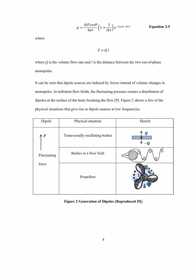
It can be seen that dipole sources are induced by forces instead of volume changes in
monopoles. In turbulent flow fields, the fluctuating pressure creates a distribution of
dipoles at the surface of the body breaking the flow [9]. Figure 2 shows a few of the
physical situations that give rise to dipole sources at low frequencies.
Dipole Physical situation Sketch
Transversally oscillating bodies
Bodies in a flow field
Propellers
Figure 2 Generation of Dipoles (Reproduced [9])
Fluctuating
force
Page 23
8/9/2019 Simulation of Whistle Noise Using Computational Fluid Dynamics
http://slidepdf.com/reader/full/simulation-of-whistle-noise-using-computational-fluid-dynamics 23/127
9
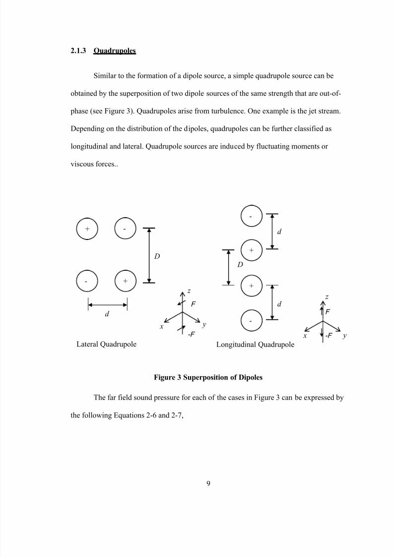
2.1.3 Quadrupoles
Similar to the formation of a dipole source, a simple quadrupole source can be
obtained by the superposition of two dipole sources of the same strength that are out-of-
phase (see Figure 3). Quadrupoles arise from turbulence. One example is the jet stream.
Depending on the distribution of the dipoles, quadrupoles can be further classified as
longitudinal and lateral. Quadrupole sources are induced by fluctuating moments or
viscous forces..
Figure 3 Superposition of Dipoles
The far field sound pressure for each of the cases in Figure 3 can be expressed by
the following Equations 2-6 and 2-7,
+ -
- +
-
+
+
-
D D
d
d
d
Lateral Quadrupole Longitudinal Quadrupole
z
x y
z
x
F
-F
F
-F y
Page 24
8/9/2019 Simulation of Whistle Noise Using Computational Fluid Dynamics
http://slidepdf.com/reader/full/simulation-of-whistle-noise-using-computational-fluid-dynamics 24/127
10
Equation 2-6
Equation 2-7
where
and are the angles the vector r makes with z-axis and x-axis in spherical coordinates
(see Figure 3).
2.2 Vortex shedding
In aeroacoustics, unwanted tones are usually caused by vortex shedding. As seen in
Figure 4, vortex induced noise can be found in many locations around a vehicle body. At
(a) type locations such as the windshield base and front hood edge, abrupt changes in
body geometry occur. At (b) type locations such as door gaps, air flows over cavities. At
(d) type locations such as the radio antenna, air flows over a cylinder. Separated flow
exists at each of these locations and vortex shedding may occur depending on the flow
conditions.
Page 25
8/9/2019 Simulation of Whistle Noise Using Computational Fluid Dynamics
http://slidepdf.com/reader/full/simulation-of-whistle-noise-using-computational-fluid-dynamics 25/127
11
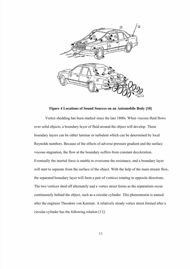
Figure 4 Locations of Sound Sources on an Automobile Body [10]
Vortex shedding has been studied since the late 1800s. When viscous fluid flows
over solid objects, a boundary layer of fluid around the object will develop. These
boundary layers can be either laminar or turbulent which can be determined by local
Reynolds numbers. Because of the effects of adverse pressure gradient and the surface
viscous stagnation, the flow at the boundary suffers from constant deceleration.
Eventually the inertial force is unable to overcome the resistance, and a boundary layer
will start to separate from the surface of the object. With the help of the main stream flow,
the separated boundary layer will form a pair of vortices rotating in opposite directions.
The two vortices shed off alternately and a vortex street forms as the separations occur
continuously behind the object, such as a circular cylinder. This phenomenon is named
after the engineer Theodore von Karman. A relatively steady vortex street formed after a
circular cylinder has the following relation [11]:
Page 26
8/9/2019 Simulation of Whistle Noise Using Computational Fluid Dynamics
http://slidepdf.com/reader/full/simulation-of-whistle-noise-using-computational-fluid-dynamics 26/127
12
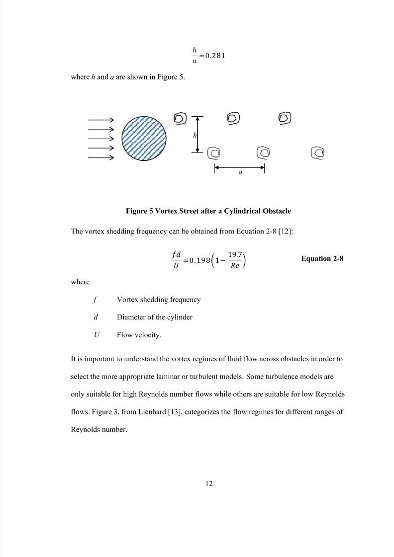
where h and a are shown in Figure 5.
Figure 5 Vortex Street after a Cylindrical Obstacle
The vortex shedding frequency can be obtained from Equation 2-8 [12]:
Equation 2-8
where
f Vortex shedding frequency
d Diameter of the cylinder
U Flow velocity.
It is important to understand the vortex regimes of fluid flow across obstacles in order to
select the more appropriate laminar or turbulent models. Some turbulence models are
only suitable for high Reynolds number flows while others are suitable for low Reynolds
flows. Figure 3, from Lienhard [13], categorizes the flow regimes for different ranges of
Reynolds number.
h
a
Page 27
8/9/2019 Simulation of Whistle Noise Using Computational Fluid Dynamics
http://slidepdf.com/reader/full/simulation-of-whistle-noise-using-computational-fluid-dynamics 27/127
13
When Re < 5, the flow is laminar and there is no vortex shedding. As the
Reynolds number increases, vortices start to appear in the flow field. When Re is in the
range of 5 to 15, a fixed pair of vortices first appears in the wake of the cylinder. As the
Reynolds number increases to about 40, the former fixed pair of vortices becomes
stretched and unstable and as a result, the first periodic driving forces begin. Laminar
vortex streets appear when Reynolds number is in the range of 40 to 150. The vortices are
laminar till Reynolds numbers exceed roughly 150. For Reynolds numbers above 300, the
flow will begin to transition from laminar to turbulent until flow is fully turbulent
between roughly 300 and 3×10
5
. Another transition takes place when Reynolds numbers
in the range of 1×10⁵ and 5×10
5. The exact Reynolds numbers for these transitions will
vary depending on the surface roughness and the free-stream turbulence level. Although
some of the regimes can be further divided into sub categories, the listed regimes and
Reynolds number ranges are sufficient to serve as guidelines for the engineers to select
the turbulence models in CFD simulation.
Page 28
8/9/2019 Simulation of Whistle Noise Using Computational Fluid Dynamics
http://slidepdf.com/reader/full/simulation-of-whistle-noise-using-computational-fluid-dynamics 28/127
14
Figure 6 Regimes of Fluid Flow across Circular Cylinders
< 5
Regime of unseparated flow
5 5 ≤ <
A fixed pair of Foppl Vortices in the
wake
≤ < And ≤ <5
Vortex Street is laminar
3≤ < 3 ×
5≤ <3
Transition range to turbulence in vortex
Vortex Street is fully turbulent
3 × < < 3 5 × 6
Laminar boundary layer has undergone
turbulent transition. The wake is narrower
and disorganized.
No vortex street is apparent
35×6 ≤ < ∞ ? Re-establishment of the turbulent
vortex street that was evident in
3≤ < 3 × . This time the boundary layer isturbulent and the wake is
thinner.
Page 29
8/9/2019 Simulation of Whistle Noise Using Computational Fluid Dynamics
http://slidepdf.com/reader/full/simulation-of-whistle-noise-using-computational-fluid-dynamics 29/127
15
2.3 Sound induced by vortex shedding
The first quantitative study of sound induced by vortex shedding was published
by Strouhal in 1878. Since then, theoretical models have been developed for predicting
the sound generated from flow over cylinders. This part of the thesis serves as a review of
the predictions of sound generated by vortex shedding of flow over cylinders.
Figure 7 Relf's Motor Driven Apparatus
In Strouhal’s experiment, the apparatus he used looks similar to Relf’s motor
driven wire-air current equipment [14] as shown in Figure 7. Strouhal concluded that [15]
(1) the frequency was independent of wire tension or length although the intensity did
increase with wire length, and (2) the frequency was approximately predicted by the
relationship:
Experimental Wire
Page 30
8/9/2019 Simulation of Whistle Noise Using Computational Fluid Dynamics
http://slidepdf.com/reader/full/simulation-of-whistle-noise-using-computational-fluid-dynamics 30/127
16
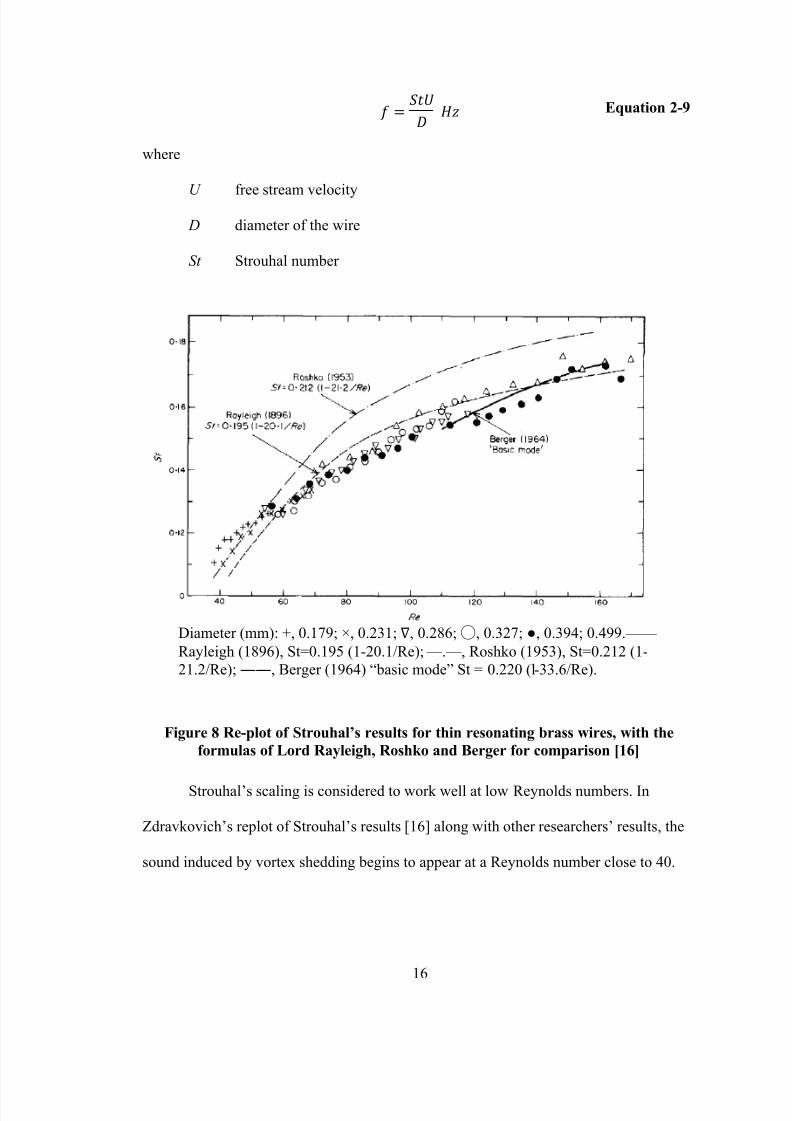
Equation 2-9
where
U free stream velocity
D diameter of the wire
St Strouhal number
Figure 8 Re-plot of Strouhal’s results for thin resonating brass wires, with the
formulas of Lord Rayleigh, Roshko and Berger for comparison [16]
Strouhal’s scaling is considered to work well at low Reynolds numbers. In
Zdravkovich’s replot of Strouhal’s results [16] along with other researchers’ results, the
sound induced by vortex shedding begins to appear at a Reynolds number close to 40.
Diameter (mm): +, 0.179; ×, 0.231; ∇, 0.286;◯, 0.327; ●, 0.394; 0.499.——
Rayleigh (1896), St=0.195 (1-20.1/Re); — . — , Roshko (1953), St=0.212 (1-
21.2/Re); ――, Berger (1964) “basic mode” St = 0.220 (l-33.6/Re).
Page 31
8/9/2019 Simulation of Whistle Noise Using Computational Fluid Dynamics
http://slidepdf.com/reader/full/simulation-of-whistle-noise-using-computational-fluid-dynamics 31/127
17
Lord Reyleigh’s [17] empirical equation matches well with Strouhal’s data acquired for a
rod with a diameter of 0.499 mm (see Figure 8).
Stowell and Deming [18] continued Strouhal’s work by measuring the sound
pressure distribution of the rotating rods. The data of the double-lobed pattern shown in
Figure 9 was obtained at 2800 rpm with rods length of 0.4572 m. They also discovered
that sound power can be related to the tip velocity and the length of the rod via
where U is the tip velocity and L is the length of the rod.
Figure 9 Polar distribution of sound pressure about rotating rod. Solid curve,
observed; dotted curve, computed. [18]
A number of measurement studies were performed after the publication of
Lighthill’s [2] aerodynamic theory in order to validate the theory. In most cases, sound
power, correlation length, and oscillating forces were measured simultaneously. Leehey
and Hanson [19] measured the sound radiated by a wire in a low-turbulence open jet
Page 32
8/9/2019 Simulation of Whistle Noise Using Computational Fluid Dynamics
http://slidepdf.com/reader/full/simulation-of-whistle-noise-using-computational-fluid-dynamics 32/127
18
wind tunnel. They also measured the lift coefficient and the vibration forces. Leehey and
Hanson’s measured sound radiation result is within 3 dB of the theoretical prediction.
Accordingly, the theoretical formula (Equation 3 in [19]) for sound radiated
aerodynamically into a free space was verified in their study.
2.4 Lighthill Analogy
In 1952, a paper named on sound generated aerodynamically, I. General theory
by Dr. Michael James Lighthill was published. In this paper, he derived a set of formulas
which were later named after him. Researchers in acoustics often regard the first
appearance of his theory as the birth of aeroacoustics. Thereafter, aeroacoustics has
become a branch of acoustics which studies the sound induced by aerodynamic activities
or fluid flow. In 60 years of time, the theory of aeroacoustics has been greatly developed
and widely applied in modern engineering fields.
The subject of Lighthill’s paper is sound generated aerodynamically, a byproduct
of an airflow and distinct from sound produced by vibration of solids. The general
problem he discussed in the paper was to estimate the radiated sound from a given
fluctuating fluid flow. There are two major assumptions. The first assumption is that the
acoustic propagation of fluctuations in the flow is not considered. The second one is the
preclusion of the back-reaction of the sound produced on the flow field itself. Therefore,
the effects of solid boundaries are neglected. However, the back-reaction is only
anticipated when there is a resonator (i.e. a cavity) close to the flow field. Accordingly,
his theory is applicable to most engineering problems. Furthermore, his theory is
confined in its application to subsonic flows, and should not be used to analyze the
transition to supersonic flow.
Page 33
8/9/2019 Simulation of Whistle Noise Using Computational Fluid Dynamics
http://slidepdf.com/reader/full/simulation-of-whistle-noise-using-computational-fluid-dynamics 33/127
19
Lighthill examined a limited volume of a fluctuating fluid flow in a very large
volume of fluid. The remainder of the fluid is assumed to be at rest. He then compared
the equations governing the fluctuations of density in the real fluid with a uniform
acoustic medium at rest, which coincides with the real fluid outside the region of flow. A
force field is acquired by calculating the difference between the fluctuating part and the
stationary part. This force field is applied to the acoustic medium and then acoustic
metrics can be predicted away from the source by solving Helmholtz equation.
Helmholtz equation can be solved easily if a free field is assumed or can be solved using
numerical simulation.
There are two significant advantages in this analogy as mentioned in his paper.
First, since we are not concerned with the back-reaction of the sound on the flow, it is
appropriate to consider the sound as produced by the fluctuating flow after the manner of
a forced oscillation. Secondly, it is best to take the free system, on which the forcing is
considered to occur, as a uniform acoustic medium at rest. Otherwise, it would be
necessary to consider the modifications due to convection with the turbulent flow and
wave propagation at different speeds within the, which would be difficult to handle.
Using the method just described, an equivalent external force field is used to describe the
acoustic source generation in the fluid [2].
2.4.1 Development of Lighthill’s Analogy
The continuity and momentum equations for a fluid can be expressed as:
0
i
i
v xt
Equation 2-10
Page 34
8/9/2019 Simulation of Whistle Noise Using Computational Fluid Dynamics
http://slidepdf.com/reader/full/simulation-of-whistle-noise-using-computational-fluid-dynamics 34/127
20
0
ij ji
j
i pvv x
vt
Equation 2-11
Here is the density, iv is the velocity in the direction i x . ij p
represents the
compressive stress tensor. iv and jv are the velocity components in two directions. ij p is
expressed as below:
p p ijijij Equation 2-12
ij
k
k
i
j
j
iij
x
v
x
v
x
v
3
2 Equation 2-13
where p is the statistic pressure of the flow field, ij is Kronecker's delta and is the
dynamic viscosity.
Now, eliminate the momentum density iv from the Equations 2-3 and 2-4 by
subtracting the gradient of the momentum equation from the time derivative of the
continuity equation. It is straightforward to obtain
ij ji
ji
pvv x xt
2
2
2
Equation 2-14
where pij represents the pressure acting on the fluid.
Next, subtract2
22
0
i xc
from both sides of Equation 2-7, this results in
ijij ji
jii
c pvv x x x
ct
2
0
2
2
2
2
02
2
Equation 2-15
Page 35
8/9/2019 Simulation of Whistle Noise Using Computational Fluid Dynamics
http://slidepdf.com/reader/full/simulation-of-whistle-noise-using-computational-fluid-dynamics 35/127
21
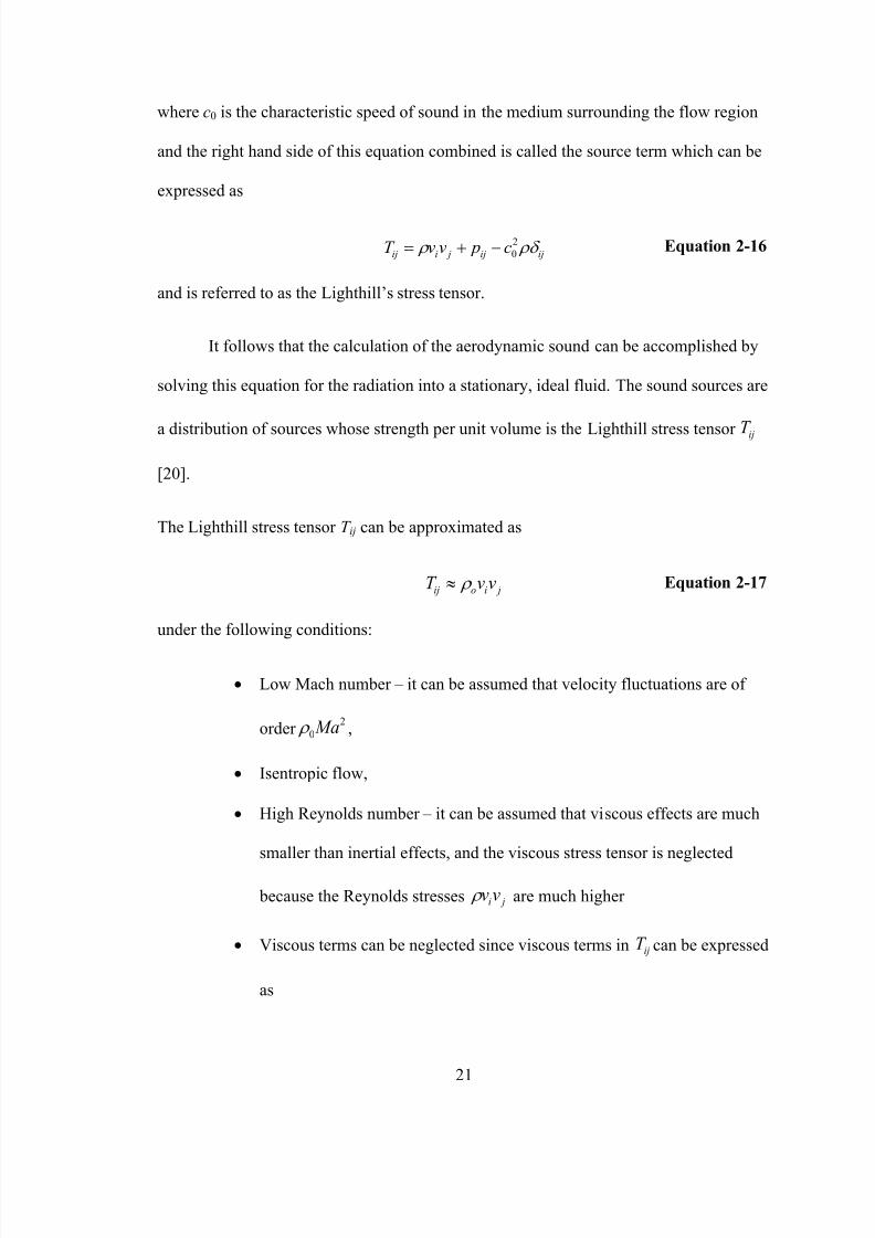
where c0 is the characteristic speed of sound in the medium surrounding the flow region
and the right hand side of this equation combined is called the source term which can be
expressed as
ijij jiij c pvvT 2
0
Equation 2-16
and is referred to as the Lighthill’s stress tensor.
It follows that the calculation of the aerodynamic sound can be accomplished by
solving this equation for the radiation into a stationary, ideal fluid. The sound sources are
a distribution of sources whose strength per unit volume is the Lighthill stress tensor ijT
[20].
The Lighthill stress tensor T ij can be approximated as
jioij vvT Equation 2-17
under the following conditions:
Low Mach number – it can be assumed that velocity fluctuations are of
order 2
0 Ma ,
Isentropic flow,
High Reynolds number – it can be assumed that viscous effects are much
smaller than inertial effects, and the viscous stress tensor is neglected
because the Reynolds stresses jivv are much higher
Viscous terms can be neglected since viscous terms in ijT can be expressed
as
Page 36
8/9/2019 Simulation of Whistle Noise Using Computational Fluid Dynamics
http://slidepdf.com/reader/full/simulation-of-whistle-noise-using-computational-fluid-dynamics 36/127
22
j
iij
x
v
, so that
ji j
i
ji
ij
x x x
v
x x
T
32
, corresponding to an octupole
source (a very ineffective sound radiator) [21].
In the frequency domain, Lighthill’s equation is written as [22]:
ji
ij
i x x
T
xa
2
2
22
0
2 Equation 2-18
A transformed potential is then used so that the finite element formulation for the
aeroacoustic analogy is compatible with the formulation for the acoustic wave
propagation. Accordingly,
2c
i Equation 2-19
where
p pca
s
22
0
(Stokesian perfect gas)
is a transformed variable [22] in the Helmholtz equation and γ represents the ratio of
specific heats.
An alternative equation for Lighthill’s analogy can be obtained by inserting Equation 2-
19 to Equation 2-18:
ji
ij
i x x
T
i xc
2
2
2
2
21
Equation 2-20
Oberai et al. (2000) developed a variational formulation of Lighthill’s analogy
which can be expressed as:
Page 37
8/9/2019 Simulation of Whistle Noise Using Computational Fluid Dynamics
http://slidepdf.com/reader/full/simulation-of-whistle-noise-using-computational-fluid-dynamics 37/127
Page 38
8/9/2019 Simulation of Whistle Noise Using Computational Fluid Dynamics
http://slidepdf.com/reader/full/simulation-of-whistle-noise-using-computational-fluid-dynamics 38/127
24
The k model is a semi-empirical turbulence model. The initial idea of
developing this model was to improve the mixing-length hypothesis and to avoid
prescribing the turbulence length scale algebraically. There are two equations in this
model, the k equation and the equation. k represents turbulence kinetic energy and
represents the dissipation rate. They can be obtained by solving the following transport
equations [24]:
j
i
i
j
j
it
ik
t
ii
i
x
u
x
u
x
u
x
k
x x
k u
t
k Equation 2-24
k
c x
u
x
u
x
u
k
c
x x x
k u
t i
j
j
i
j
it
k
t
k k
k
2
2
1
Equation 2-25
where t is called turbulent viscosity and
/2k ct Equation 2-26
The constants ,,,,21 k ccc are respectively 1.44, 1.92, 0.09, 1.0, and 1.3. However,
with the given values, the model is only suitable for high Reynolds flow, which works
well if the flow is fully developed and is sufficiently spaced from wall boundaries. To
improve the performance of the model in the near wall fields, wall functions can be used
to model boundary effects.
2.5.2
model
The turbulence model was first introduced by Kolmogorov in 1942 [25].
Similar to the k-ε turbulence model, the turbulence model is also a two-equation
turbulence model. The first turbulence parameter in this model is the kinetic energy term,
Page 39
8/9/2019 Simulation of Whistle Noise Using Computational Fluid Dynamics
http://slidepdf.com/reader/full/simulation-of-whistle-noise-using-computational-fluid-dynamics 39/127
25
k , which is also used in the model. Instead of using ε, the dissipation per unit mass,
ω, the dissipation per unit turbulence kinetic energy, was chosen as the second turbulence
parameter. Since the introduction of the
turbulence model, it has been improved by
several researchers. Nowadays, the most widely used turbulence model is based on
Wilcox et al.’s work [26] [27] [28].
In Wilcox’s k-ω turbulence model [29], eddy viscosity is expressed as:
Equation 2-27
Turbulence kinetic energy and specific dissipation rate can be obtained by solving the
following transport equations:
Equation 2-28
Equation 2-29
where the closure coefficients are
5
3
Page 40
8/9/2019 Simulation of Whistle Noise Using Computational Fluid Dynamics
http://slidepdf.com/reader/full/simulation-of-whistle-noise-using-computational-fluid-dynamics 40/127
26
with the auxiliary relations
The closure coefficients are used to replace unknown double and triple correlations with
algebraic expressions involving known turbulence and mean-flow properties as proposed
by Wilcox [29]. These values are determined based on experimental results.
The
turbulence model performs better at near wall layers than the
turbulence model, and has been successfully applied for flows with moderate adverse
pressure gradients. However, it still has trouble dealing with pressure induced separation
[30]. One major disadvantage of the standard turbulence model is that the
sensitivity of its ω equation is strongly related to the values of in the free stream
outside the boundary layer [31]. Although the near wall performance is superior, this
major flaw prevents the turbulence model from replacing the turbulence
model [32]. This led to the development of the shear stress transport (SST)
turbulence model.
The SST turbulence model [30] is a two equation eddy-viscosity model
like the model. The advantage of the shear stress transport (SST) formulation is
that it combines both
and
turbulence models. When dealing with the free
stream flow, the SST formulation will use the ε behavior to avoid the excessive free
stream sensitivity from which the original turbulence model suffers. Furthermore,
the advantage of the turbulence model is preserved so the model works well close
Page 41
8/9/2019 Simulation of Whistle Noise Using Computational Fluid Dynamics
http://slidepdf.com/reader/full/simulation-of-whistle-noise-using-computational-fluid-dynamics 41/127
Page 42
8/9/2019 Simulation of Whistle Noise Using Computational Fluid Dynamics
http://slidepdf.com/reader/full/simulation-of-whistle-noise-using-computational-fluid-dynamics 42/127
28
3 3
√ 5
√
5
Notice that the constants of are the same as those in the k-ε turbulence model.
2.5.3 Large Eddy Simulation
The Large Eddy Simulation (LES) turbulence model is a “hybrid” approach. In
LES, the large motions are directly computed but the small eddies are usually
approximated using a model [34]. . It is the most widely used model in academia, but it is
still not popular in industrial applications. One of the reasons is that the near wall region
needs to be represented with an extremely fine mesh not only in the direction
perpendicular to the wall but also parallel with the wall. For this reason, LES is not
recommended with flows with strong wall boundary effects. In other words, the flow
should be irrelevant to the wall boundary layers. Another disadvantage of the LES
turbulence model is the excessive computational power needed due to the statistical
stability requirement. Generally, the LES solver requires long computational times to
Page 43
8/9/2019 Simulation of Whistle Noise Using Computational Fluid Dynamics
http://slidepdf.com/reader/full/simulation-of-whistle-noise-using-computational-fluid-dynamics 43/127
29
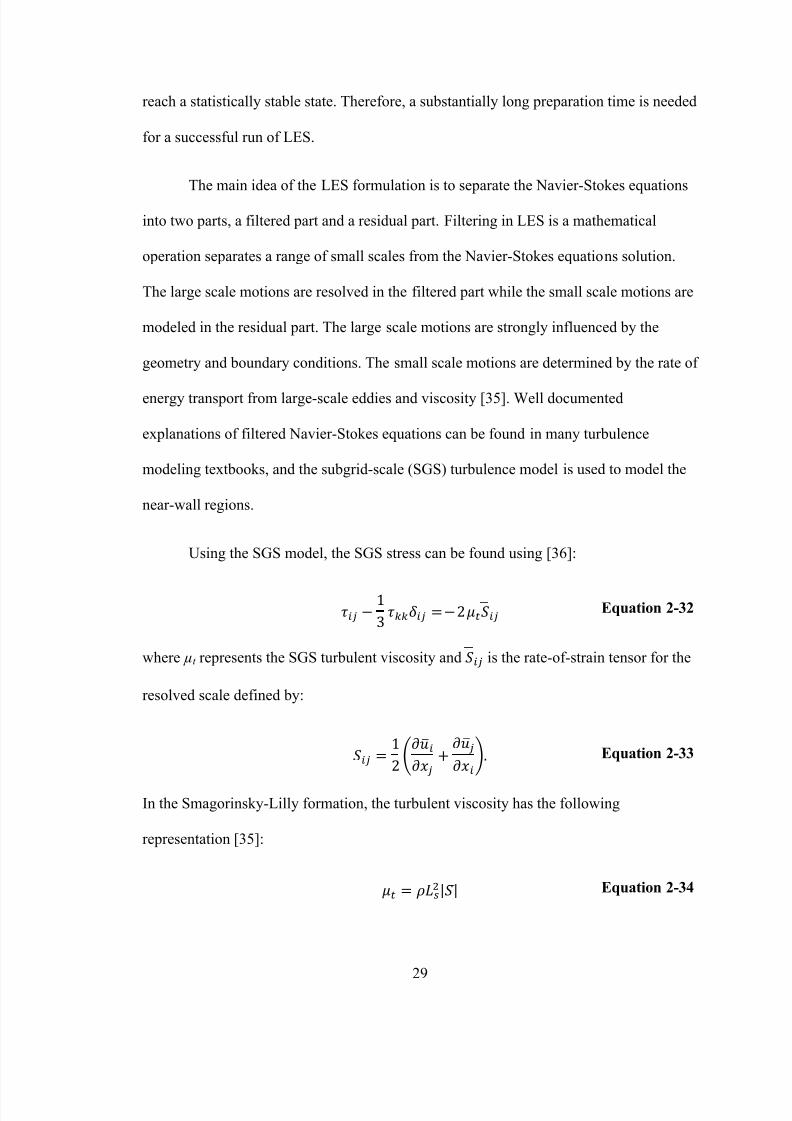
reach a statistically stable state. Therefore, a substantially long preparation time is needed
for a successful run of LES.
The main idea of the LES formulation is to separate the Navier-Stokes equations
into two parts, a filtered part and a residual part. Filtering in LES is a mathematical
operation separates a range of small scales from the Navier-Stokes equations solution.
The large scale motions are resolved in the filtered part while the small scale motions are
modeled in the residual part. The large scale motions are strongly influenced by the
geometry and boundary conditions. The small scale motions are determined by the rate of
energy transport from large-scale eddies and viscosity [35]. Well documented
explanations of filtered Navier-Stokes equations can be found in many turbulence
modeling textbooks, and the subgrid-scale (SGS) turbulence model is used to model the
near-wall regions.
Using the SGS model, the SGS stress can be found using [36]:
3 Equation 2-32
where µt represents the SGS turbulent viscosity and is the rate-of-strain tensor for the
resolved scale defined by:
Equation 2-33
In the Smagorinsky-Lilly formation, the turbulent viscosity has the following
representation [35]:
| |̅ Equation 2-34
Page 44
8/9/2019 Simulation of Whistle Noise Using Computational Fluid Dynamics
http://slidepdf.com/reader/full/simulation-of-whistle-noise-using-computational-fluid-dynamics 44/127
30
Equation 2-35
where L s is the mixing length for subgrid scales and is computed as:
where
and
d distance to the closest wall
C s Smagorinsky constant
V volume of the computational cell.
2.6 Acoustic FEM
2.6.1 Introduction
There are two major types of numerical methods in acoustics: the boundary
element method (BEM) and finite element method (FEM). Although noise control
engineering primarily depends on measurement and experience, numerical methods have
been used to predict noise in the early design stage as a means to lower the cost of design
by increasing design efficiency [37]. Normally, acoustic FEM is used to solve interior
problems, but nowadays FEM can be used to solve acoustic radiation problems with the
advent of infinite elements.
The Helmholtz equation is the governing equation for linear acoustics and can be
expressed as
Page 45
8/9/2019 Simulation of Whistle Noise Using Computational Fluid Dynamics
http://slidepdf.com/reader/full/simulation-of-whistle-noise-using-computational-fluid-dynamics 45/127
31
∇ Equation 2-36
where p is the sound pressure and k is the wavenumber.
Multiply Equation 2-36 by a weighting function and integrate the resulting equation
by parts. Then, the weak form of the linear Helmholtz equation can be expressed as
∫∇ ∇ ∫
∫
Equation 2-37
By applying the natural and general natural boundary conditions, Equation 2-30 becomes
∫ ∇ ∇
∫
∫ ∫
Equation 2-38
According to the Galerkin approach, p and can be approximated by using a linear
combination of shape functions N i and W L:
[]{} Equation 2-39
[]{} Equation 2-40
By substituting p and into equation 2-38, the finite element equation can be expressed
as
Page 46
8/9/2019 Simulation of Whistle Noise Using Computational Fluid Dynamics
http://slidepdf.com/reader/full/simulation-of-whistle-noise-using-computational-fluid-dynamics 46/127
32
∫ ∇ [ ] ∇{}
∫ []{}
∫[]{} {} ∫[]{}
Equation 2-41
2.6.2 Infinite Element
An infinite element is a finite element that covers a semi-infinite sector of space
[38]. It was developed in the interest of solving radiation problems. The solution of the
wave equation using infinite elements is based on multipole expansion. The method used
in ACTRAN is reviewed in this chapter. More detailed information can be found in
ACTRAN User’s Guide Volume 1.
Consider the convected wave equation in the local coordinate system ( Equation 2-42
The above equation can be further simplified to the Helmholtz equation using Prandtl-
Glauert transformation. The resulting equation is expressed as follows:
Equation 2-43
where
Page 47
8/9/2019 Simulation of Whistle Noise Using Computational Fluid Dynamics
http://slidepdf.com/reader/full/simulation-of-whistle-noise-using-computational-fluid-dynamics 47/127
Page 48
8/9/2019 Simulation of Whistle Noise Using Computational Fluid Dynamics
http://slidepdf.com/reader/full/simulation-of-whistle-noise-using-computational-fluid-dynamics 48/127
34
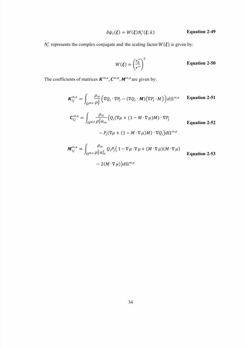
Equation 2-49
represents the complex conjugate and the scaling factor is given by:
Equation 2-50
The coefficients of matrices are given by:
∫ ∇ ∇ ∇ (∇ ) Equation 2-51
∫
(∇ ∇ ∇ ∇ ∇ ∇)
Equation 2-52
∫ ( ∇ ∇ ∇ ∇ ∇ )
Equation 2-53
Page 49
8/9/2019 Simulation of Whistle Noise Using Computational Fluid Dynamics
http://slidepdf.com/reader/full/simulation-of-whistle-noise-using-computational-fluid-dynamics 49/127
Page 50
8/9/2019 Simulation of Whistle Noise Using Computational Fluid Dynamics
http://slidepdf.com/reader/full/simulation-of-whistle-noise-using-computational-fluid-dynamics 50/127
36
This would require a very large mesh. Secondly, the procedure is computationally
expensive since it requires finer meshes, long transient computations in the statistical
steady state, and pressure scale limits.
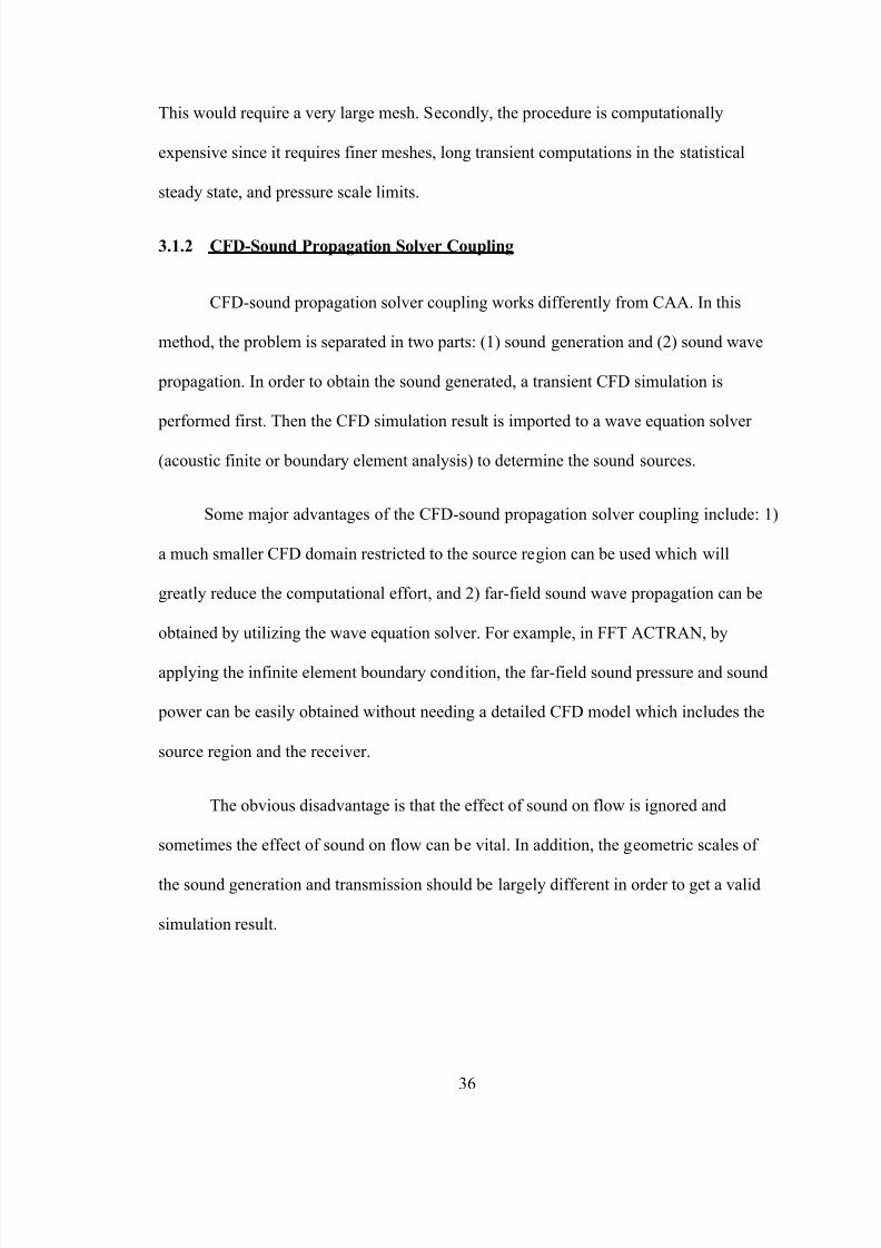
3.1.2 CFD-Sound Propagation Solver Coupling
CFD-sound propagation solver coupling works differently from CAA. In this
method, the problem is separated in two parts: (1) sound generation and (2) sound wave
propagation. In order to obtain the sound generated, a transient CFD simulation is
performed first. Then the CFD simulation result is imported to a wave equation solver
(acoustic finite or boundary element analysis) to determine the sound sources.
Some major advantages of the CFD-sound propagation solver coupling include: 1)
a much smaller CFD domain restricted to the source region can be used which will
greatly reduce the computational effort, and 2) far-field sound wave propagation can be
obtained by utilizing the wave equation solver. For example, in FFT ACTRAN, by
applying the infinite element boundary condition, the far-field sound pressure and sound
power can be easily obtained without needing a detailed CFD model which includes the
source region and the receiver.
The obvious disadvantage is that the effect of sound on flow is ignored and
sometimes the effect of sound on flow can be vital. In addition, the geometric scales of
the sound generation and transmission should be largely different in order to get a valid
simulation result.
Page 51
8/9/2019 Simulation of Whistle Noise Using Computational Fluid Dynamics
http://slidepdf.com/reader/full/simulation-of-whistle-noise-using-computational-fluid-dynamics 51/127
37
3.1.3 Broadband Noise Sources Models
It is well known that the Transient CFD solutions are CPU intensive. However, if
no specific tones are expected, broadband noise sources models can be utilized and the
transient CFD solution can be avoided. Instead, only a steady state CFD solution is
required. With the help of analytical models such as Lilley’s acoustic source strength
broadband noise model [40], the strength of the sound sources can be obtained with good
accuracy. Those sound sources can be applied directly to an acoustic BEM or FEM
model.
3.2 General Assumptions
3.2.1 Model Dimension
The models used in this thesis are all 2-D models. Studies have shown that 2-D
models for symmetric geometry work well in aeroacoustic simulations. Takahashi et al.
[41] have shown that identical results can be obtained using 2-D and 3-D models for the
edge tone problem (see Figure 10). The peaks in acoustic frequency spectrum compare
especially well between both 2-D and 3-D models. They have concluded that the 2-D
approximation is adequate for determining the tones due to flow noise. Additionally,
Rubio et al. [42]has performed an aeroacoustic simulation of a 2-D expansion chamber,
and found that phenomenon that could be modeled in 2-D governed the tonal noise.
However, a 3-D model was necessary to accurately predict the broadband noise due to
turbulence.
Page 52
8/9/2019 Simulation of Whistle Noise Using Computational Fluid Dynamics
http://slidepdf.com/reader/full/simulation-of-whistle-noise-using-computational-fluid-dynamics 52/127
Page 53
8/9/2019 Simulation of Whistle Noise Using Computational Fluid Dynamics
http://slidepdf.com/reader/full/simulation-of-whistle-noise-using-computational-fluid-dynamics 53/127
39
agreed Mach number threshold for CFD solutions aimed at identifying aeroacoustic
sources.
3.2.3 Interactions and Feedbacks
Fluid-structure interaction is the interaction of some movable or deformable
structure with an internal or surrounding fluid flow [46]. One infamous example of this
type of interaction is the failure of the Tacoma Narrows Bridge in 1940. In aeroacoustics,
this type of interaction is often disregarded because of the complexity of structure and
fluid solver coupling.
There is no fluid-structure interaction considered in this thesis though the fluid-
structure interaction can be vital in certain cases such as the vibration of fan blades and
flow over cylinders. This kind of interaction is more likely to occur when the frequency
of turbulence is close to the natural frequency of the structure and therefore generates
sound in greater amplitude. In this thesis, we focus on the sound generated by fluid flow
only and therefore we assume all structures are perfectly rigid.
Aeroacoustic feedback occurs when the sound wave generated from the fluid flow
positively affects the flow field and therefore establishes a self-excited system. This
aeroacoustic feedback loop plays an important role in certain cases such as flow over a
cavity and flow at a sharp edge, and will cause an increase in the sound amplitude.
However, most CFD solvers are unable to model this interaction due to the difference in
scales. There are orders of magnitude difference in pressure and velocity between CFD
and acoustics. For example, the acoustic wave in air travels at 343 m/s under normal
conditions while low sub sonic flow is at least two orders of magnitude lower. Typically,
Page 54
8/9/2019 Simulation of Whistle Noise Using Computational Fluid Dynamics
http://slidepdf.com/reader/full/simulation-of-whistle-noise-using-computational-fluid-dynamics 54/127
40
CFD solvers have inherent dissipation to ensure stability and are therefore unable to
handle these interactions.
3.3 CFD-Sound Propagation Solver Coupling Process
The aeroacoustic simulation in a CFD-sound propagation solver coupling process is
based on variables such as the pressure and density fields computed by a CFD solver
during transient flow simulation. Figure 11 shows the solution process of this solver
coupling approach. The aeroacoustic solver will read in the transient CFD solution data
and compute the aeroacoustic sources in the time domain. Then a Fast Fourier Transform
is conducted in order to obtain the source data in the frequency domain. After the
frequency domain sources are computed, an acoustic simulation can be performed.
Figure 11 CFD-Sound Propagation Solver Coupling Solution Process
CFD Mesh
CFD Simulation
Sources
(Time Domain)
Acoustic Mesh
Acoustic Simulation
A c o u s t i c
A n a l o g y
FFT
Source Mapping
Acoustic Result
Page 55
8/9/2019 Simulation of Whistle Noise Using Computational Fluid Dynamics
http://slidepdf.com/reader/full/simulation-of-whistle-noise-using-computational-fluid-dynamics 55/127
41
3.3.1 Comments on Source Mapping
Two methods are available to accomplish the source mapping from the CFD
domain to the acoustic domain: 1) linear interpolation and 2) conservative integration.
In linear interpolation, all nodal coordinates’ acoustic values are sampled in the
CFD mesh, and are projected to the closest node on the acoustic mesh. Loss of
information may occur during this process if the acoustic mesh is coarser than the CFD
mesh (Figure 12).
Figure 12 Linear Interpolation Source Projection Method
Conservative integration overcomes this difficulty. The aeroacoustic field is
integrated using the shape functions of the acoustic mesh. Accordingly, all aeroacoustic
sources are preserved (Figure 13).
Loss of Information
Linear Interpolation from
CFD mesh to Acoustic Node
No Acoustic Node for Projection
Page 56
8/9/2019 Simulation of Whistle Noise Using Computational Fluid Dynamics
http://slidepdf.com/reader/full/simulation-of-whistle-noise-using-computational-fluid-dynamics 56/127
42
Figure 13 Conservative Integration Source Projection Method
3.4 Fast Fourier Transform for Aeroacoustic Simulation
The acoustic simulation is in the frequency domain, while the CFD transient
solution is in time domain. Hence, aeroacoustic sources computed from the CFD solution
must be transformed to the frequency domain using a Fast Fourier Transform. The Fast
Fourier Transform follows the general FFT rules including the Nyquist requirement. Thus,
the time step size and number of samples in time domain will affect the frequency
resolution in frequency domain.
3.4.1 Determine Time Step Size and Number of Time Steps for CFD Simulation
Before the CFD simulation, the maximum frequency of the aeroacoustic result,
sampling frequency should be set to the maximum frequency of interest. Additionally, if
tones are expected, the sampling frequency needs to be at least 10 to 20 times greater
Acoustic Nodes
CFD Nodes
Conservative Integrationfrom CFD Nodes to CFD
mesh Using Acoustic Mesh
Shape Functions
Page 57
8/9/2019 Simulation of Whistle Noise Using Computational Fluid Dynamics
http://slidepdf.com/reader/full/simulation-of-whistle-noise-using-computational-fluid-dynamics 57/127
43
than the highest frequency of the tones of interest. Accordingly, the time step size of the
CFD simulation can be obtained using the following relation,
× Equation 3-1
× Equation 3-2
Notice that sampling frequency is multiplied by 2 due to the Nyquist requirement.
3.5 Wall Boundary Meshing Requirements
A successful CFD simulation often requires a CFD mesh with great quality. It is
essential to have a mesh representing the shape of the geometry accurately. Additionally,
the near wall region needs to be handled with care because turbulent flows are largely
affected by the presence of the wall boundaries where rapid changes of flow variables
such as pressure gradients take place. In the modeling process, the dimensionless wall
distance ( y+) is often used in the estimation of the actual boundary thickness and can be
used to guide the selection of an appropriate near wall treatment. y+ can be read as the
ratio of the turbulent and laminar effects in a cell.
A dimensionless wall distance is defined by the following formula:
Equation 3-3
where
friction velocity (shear velocity) at the closest wall
y distance to the closest wall
ν local kinematic viscosity of the fluid
Page 58
8/9/2019 Simulation of Whistle Noise Using Computational Fluid Dynamics
http://slidepdf.com/reader/full/simulation-of-whistle-noise-using-computational-fluid-dynamics 58/127
Page 59
8/9/2019 Simulation of Whistle Noise Using Computational Fluid Dynamics
http://slidepdf.com/reader/full/simulation-of-whistle-noise-using-computational-fluid-dynamics 59/127
Page 60
8/9/2019 Simulation of Whistle Noise Using Computational Fluid Dynamics
http://slidepdf.com/reader/full/simulation-of-whistle-noise-using-computational-fluid-dynamics 60/127
Page 61
8/9/2019 Simulation of Whistle Noise Using Computational Fluid Dynamics
http://slidepdf.com/reader/full/simulation-of-whistle-noise-using-computational-fluid-dynamics 61/127
Page 62
8/9/2019 Simulation of Whistle Noise Using Computational Fluid Dynamics
http://slidepdf.com/reader/full/simulation-of-whistle-noise-using-computational-fluid-dynamics 62/127
48
Chapter 4
Verification of Simulation Approach
4.1 Lid-Driven Test Case for Mesh Selection
4.1.1 CFD Mesh Types
There are three types of mesh strategies used in CFD simulations: structured
meshes, unstructured meshes, and hybrid meshes. A mesh is called structured if the node
connectivity has a fixed pattern. Structured meshes are usually easy to generate for
regular geometries (see Figure 16). A mesh is unstructured if the connectivities of the
nodes are irregular. More space is required to store the unstructured mesh because there
is no fixed pattern neighborhood connectivity (see Figure 17). An unstructured mesh
usually requires less effort as it can be generated using automatic meshers. A “hybrid”
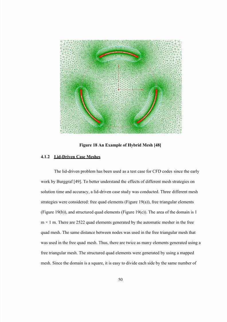
mesh is a combination of both structured and unstructured domains. Figure 18 shows an
example where the area close to the blades is represented with a structured mesh while
the regions away from the blades are unstructured. The advantage of a hybrid mesh is that
a structured mesh can be used in regions where more detail and accuracy are needed
whereas a coarser unstructured mesh is viable away from the blades.
Page 63
8/9/2019 Simulation of Whistle Noise Using Computational Fluid Dynamics
http://slidepdf.com/reader/full/simulation-of-whistle-noise-using-computational-fluid-dynamics 63/127
Page 64
8/9/2019 Simulation of Whistle Noise Using Computational Fluid Dynamics
http://slidepdf.com/reader/full/simulation-of-whistle-noise-using-computational-fluid-dynamics 64/127
50
Figure 18 An Example of Hybrid Mesh [48]
4.1.2 Lid-Driven Case Meshes
The lid-driven problem has been used as a test case for CFD codes since the early
work by Burggraf [49]. To better understand the effects of different mesh strategies on
solution time and accuracy, a lid-driven case study was conducted. Three different mesh
strategies were considered: free quad elements (Figure 19(a)), free triangular elements
(Figure 19(b)), and structured quad elements (Figure 19(c)). The area of the domain is 1
m × 1 m. There are 2522 quad elements generated by the automatic mesher in the free
quad mesh. The same distance between nodes was used in the free triangular mesh that
was used in the free quad mesh. Thus, there are twice as many elements generated using a
free triangular mesh. The structured quad elements were generated by using a mapped
mesh. Since the domain is a square, it is easy to divide each side by the same number of
Page 65
8/9/2019 Simulation of Whistle Noise Using Computational Fluid Dynamics
http://slidepdf.com/reader/full/simulation-of-whistle-noise-using-computational-fluid-dynamics 65/127
51
divisions. In this case, there are 50 divisions on each side making a total of 2500
structured quad elements.
Figure 19 Meshes Used in Lid-Driven Case
4.1.3 CFD Simulation Setup
The standard lid-driven problem is a 2-D square domain with fluid and Dirichlet
boundary conditions. A Dirichlet boundary condition specifies the values of the solution
on the boundary of the computational domain of an ordinary or a partial differential
equation. Figure 20 shows the boundary conditions of the case studied. Three out of the
four sides of the square domain are stationary, and there is only one side moving. u
represents the horizontal velocity and v represents the vertical velocity. For the case
shown here, the horizontal velocity of the lid (u) is 1 m/s.
2522 Elements 5724 Elements 2500 Elements
Free Quad Elements Free Triangular Elements Structured Quad Elements
(A) (B) (C)
Page 66
8/9/2019 Simulation of Whistle Noise Using Computational Fluid Dynamics
http://slidepdf.com/reader/full/simulation-of-whistle-noise-using-computational-fluid-dynamics 66/127
52
Figure 20 Boundary Condition of the Lid-Driven Case
The fluid used in this simulation was selected to have a density ρ = 1 kg/m3, and a
dynamic viscosity µ = 0.001 kg/ms. The reason for choosing these values is to achieve a
Reynolds number of 1000 at the moving wall. The lid-driven case at this Reynolds
number has been well studied numerically by Ghia et al. [50].
At a Reynolds number of 1000, the flow is laminar. Therefore, a laminar viscous
model is used and the steady state solution is obtained.
Scaled residuals can be good indicators of the convergence of a solution. In a
typical ANSYS FLUENT simulation case, there are three types of residuals: continuity,
velocity and solver specific residuals. If a computer has an infinite precision, the
residuals will reach zero eventually. However, in reality, computers have finite precision.
For a double precision computer, the residual can drop up to 12 orders of magnitude. A
recommended criterion of scaled continuity and velocity residual is 10-3
[6].
Page 67
8/9/2019 Simulation of Whistle Noise Using Computational Fluid Dynamics
http://slidepdf.com/reader/full/simulation-of-whistle-noise-using-computational-fluid-dynamics 67/127
53
The convergence criteria in this study are as follows:
Continuity Residual < 10-6
;
Velocity Residual < 10-3
.
4.1.4 Result and Discussion
Figures 21 and 22 show the x-component of the velocity at the vertical center line
of the domain from the bottom to the top of the domain. The results are compared to the
results of Ghia et al. [50]. Figure 21 shows the solution at the centerline while Figure 22
zooms in at the vertical position of 0.2 m.
The results from each of the three mesh strategies compare well to the previous
study which was obtained through a CFD simulation as well as can be seen from Figure
21 and Figure 22. Similarly, contour plots are shown in Figure 23 and Figure 24.
However, the difference is not significant. Since the results are nearly identical, it is
important to take a look at solution time. Both free and structured quad elements
converge in half the time as a mesh consisting of triangular elements. Figure 25 compares
the continuity residual for the three meshes. Notice that the residual decreases much more
rapidly for both quad meshes. Similarly, the friction coefficient converges in
approximately half the number of iterations (Figure 26).
Page 68
8/9/2019 Simulation of Whistle Noise Using Computational Fluid Dynamics
http://slidepdf.com/reader/full/simulation-of-whistle-noise-using-computational-fluid-dynamics 68/127
Page 69
8/9/2019 Simulation of Whistle Noise Using Computational Fluid Dynamics
http://slidepdf.com/reader/full/simulation-of-whistle-noise-using-computational-fluid-dynamics 69/127
55
Figure 23 Velocity Contour Plot (Free Quad Elements)
Figure 24 Velocity Contour Plot (Structured Quad Elements)
Page 70
8/9/2019 Simulation of Whistle Noise Using Computational Fluid Dynamics
http://slidepdf.com/reader/full/simulation-of-whistle-noise-using-computational-fluid-dynamics 70/127
56
Figure 25 Continuity Residual History
Figure 26 Friction Coefficient History (At the Moving Wall)
1.E-06
1.E-05
1.E-04
1.E-03
1.E-02
1.E-01
1.E+00
0 1000 2000 3000
C o n t i n u i t y R e s i d u a l
Iterations
Free Quad Elements
Free Triangular Elements
Structured Quad Elements
0
0.002
0.004
0.006
0.008
0.01
0.012
0.014
0 1000 2000 3000
F r i c t i o n C o e f f i c i e n t
Iterations
Free Quad Elements
Free Triangular Elements
Structured Quad Elements
Page 71
8/9/2019 Simulation of Whistle Noise Using Computational Fluid Dynamics
http://slidepdf.com/reader/full/simulation-of-whistle-noise-using-computational-fluid-dynamics 71/127
Page 72
8/9/2019 Simulation of Whistle Noise Using Computational Fluid Dynamics
http://slidepdf.com/reader/full/simulation-of-whistle-noise-using-computational-fluid-dynamics 72/127
58
quickly and there is no time for the heat exchange. The adiabatic process has the
following relation:
Equation 4-1
where γ is the ratio of specific heats.
According to Newton’s second law,
Equation 4-2
where
By replacing F and m using Equation 4-1, the following equation can be obtained:
Equation 4-3
This is a first order system and the natural frequency of this system is:
Equation 4-4
Page 73
8/9/2019 Simulation of Whistle Noise Using Computational Fluid Dynamics
http://slidepdf.com/reader/full/simulation-of-whistle-noise-using-computational-fluid-dynamics 73/127
59
Figure 27 Helmholtz Resonator and Spring-Mass Damper Analogy
L in the previous equation is now replaced with the corrected length L’ because in
reality, an additional volume outside the neck and inside the cavity moves with the
system. The resonance frequency of the Helmholtz resonator can be expressed by the
following formula:
Equation 4-5
where
L’ Corrected length of the neck
S b Cross section area of the neck
V Volume of the cavity
c Speed of sound
The corrected length of the neck [51] can be approximated as:
Neck
Cavity
Flow
M
K
F
M
x
V - S b x
P A + P
a (b)
Page 74
8/9/2019 Simulation of Whistle Noise Using Computational Fluid Dynamics
http://slidepdf.com/reader/full/simulation-of-whistle-noise-using-computational-fluid-dynamics 74/127
60
Equation 4-6
when the opening is flanged and
Equation 4-7
when the opening is in free space. L is the length (height) of the neck.
4.2.2 Geometry and Mesh
Figure 28 shows the geometry of the simulated Helmholtz resonator. The length
of each section can be found in Table 2. The geometry has three components: the free
stream area (shown in red), the resonator cavity (shown in green), and the neck
connecting the free stream area and the resonator cavity.
Figure 28 Geometry of the Simulated Helmholtz Resonator
L1
H 1
L2
H 2
D
Page 75
8/9/2019 Simulation of Whistle Noise Using Computational Fluid Dynamics
http://slidepdf.com/reader/full/simulation-of-whistle-noise-using-computational-fluid-dynamics 75/127
61
Table 2 Dimension of the Simulated Helmholtz Resonator
L1 1.5 m
H 1 0.5 m
D 0.2 m
L2 0.5 m
H 2 0.3 m
Neck Length 0.01 m
These values were recommended by ANSYS FLUENT [52] in order to achieve a
relatively low resonance frequency, and therefore requires less solution time because the
sampling frequency can be lower (See Chapter 3.4.1). The frequency of the resonator can
be calculated using Equation 4-5, and a frequency of 120 Hz is obtained.
Figure 29 Helmholtz Resonator Mesh for CFD Simulation
Page 76
8/9/2019 Simulation of Whistle Noise Using Computational Fluid Dynamics
http://slidepdf.com/reader/full/simulation-of-whistle-noise-using-computational-fluid-dynamics 76/127
62
Figure 29 shows the mesh used for the CFD simulation. All the parts of the
geometry are simple and a structured mesh was used because of the simple geometry.
The minimum element length is 2 mm while the maximum element length is 17.2 mm at
the inlet and outlet. Another coarser mesh (Figure 30) for acoustic simulation has been
made to shorten the run time needed for the acoustic calculation. A conservative
integration method is chosen to preserve the source information in the projection from the
CFD domain to the acoustic domain (see Chapter 3.3.1 for detail of source projection).
The mesh is extended at the outlet for acoustic wave propagation purposes. The element
size is uniformly 10 mm in this mesh.
Figure 30 Helmholtz Resonator Mesh for Acoustic Simulation
4.2.3 Simulation Setup and Steps
Figure 31 shows the overview of the simulation steps. The first step is to generate
the CFD mesh and setup the CFD simulation with proper boundary conditions, and a
Sources Applied
No Source Applied
Page 77
8/9/2019 Simulation of Whistle Noise Using Computational Fluid Dynamics
http://slidepdf.com/reader/full/simulation-of-whistle-noise-using-computational-fluid-dynamics 77/127
63
turbulent model. A steady state CFD computation is then performed to determine the
initial flow velocity. The steady state velocity field is then used to initialize the transient
computation. During the transient computation, the velocity and density fields are
exported at each time step. The next step is to link between the CFD simulation and
acoustic simulation by computing aeroacoustic sources from the transient CFD
simulation. A fast fourier transform is performed so that the source terms are transferred
into the frequency domain. In order to use the coarser mesh (compared to the CFD mesh)
for the acoustic simulation, the source terms are projected to the acoustic mesh and the
acoustic simulation is performed in the frequency domain. Each of these steps will now
be discussed in more detail.
Figure 31 Simulation Process
Steady State Computation
Transient Computation
CFD Mesh
and Solution SetupAcoustic Mesh
and Solution Setup
Acoustic Calculation
Radiated SoundPower
Aeroacoustic SourceComputation
FFT
Source Projection
Page 78
8/9/2019 Simulation of Whistle Noise Using Computational Fluid Dynamics
http://slidepdf.com/reader/full/simulation-of-whistle-noise-using-computational-fluid-dynamics 78/127
64
4.2.3.1 Steady State Solution
A steady state solution is first conducted in preparation for the transient
simulation. In general, the transient solution data needs to be collected until the flow is
fully established. In order to meet this requirement, analysts must run the transient flow
simulation for a very long time before exporting the solution data from each of the time
steps. Alternatively, a steady state solution can be performed and the steady state solution
data is used to initialize the transient solution from which the transient solution data is
exported. Information about the simulation setup including the turbulence model and the
boundary conditions can be found in Table 3.
A realizable with non-equilibrium wall function is selected as the
turbulence model in this simulation. The realizable k-ε model is suitable for coarse
meshes, where the wall-cell y+ values are typically 30 and above. The term “realizable”
means that the model satisfies certain mathematical constraints so that the Reynolds
stresses calculated are consistent with the real flow physics. Like the standard wall
functions, the non-equilibrium wall functions are also a two-equation approach. Unlike
the standard wall functions, the non-equilibrium wall functions are sensitized to pressure-
gradient effects [53]. SIMPLE (semi-implicit method for pressure-linked equations)
pressure-velocity coupling method is selected. The SIMPLE algorithm uses a relationship
between velocity and pressure corrections to enforce mass conservation and to obtain the
pressure field [54]. The Green-Gauss cell based method is selected for its good
performance with structured meshes as recommended by ANSYS FLUENT [52]. The
computation is initialized from the inlet which means the conditions at the inlet are first
satisfied.
Page 79
8/9/2019 Simulation of Whistle Noise Using Computational Fluid Dynamics
http://slidepdf.com/reader/full/simulation-of-whistle-noise-using-computational-fluid-dynamics 79/127
65
Table 3 Steady State Simulation Setup
Turbulence Model Realizable k-ε with non-equilibrium wall functions
Fluid Property Ideal-gas
Pressure-Velocity Coupling SIMPLE
Gradient Method Green-Gauss cell based
Inlet Velocity inlet V = 27 m/s with 1% turbulence intensity
Outlet Pressure outlet P = 1 atm with 1% turbulence intensity
Initialization Initialized from inlet
After 300 iteration, the solution converged. It can be seen in the velocity contour
plot below that two unsteady regions with high velocity magnitude have formed (see
Figure 32 circled parts). The velocity field at this point is used to initialize the transient
solution.
Figure 32 Velocity Contour Plot (Steady State)
Page 80
8/9/2019 Simulation of Whistle Noise Using Computational Fluid Dynamics
http://slidepdf.com/reader/full/simulation-of-whistle-noise-using-computational-fluid-dynamics 80/127
66
4.2.3.2 Transient Solution
A built-in ANSYS FLUENT TUI command init-instantaneous-vel provides a way
to get a more realistic instantaneous velocity field (this new velocity field is unsteady).
Transient LES simulation can be started after the issuance of this command. The setup of
LES simulation is listed in Table 4. More information about the LES simulation can be
found in Section 2.4.3. It is well known that LES requires excessively high resolution for
wall boundary layers because near the wall, the turbulence components are geometrically
very small close to the wall. As a result, standard LES is only recommended to the flow
situation where the wall boundary layers are irrelevant. However, with the help of WALE
(Wall-Adapting Local Eddy-Viscosity) model, the hardship of LES can be improved at
the boundary layers. It will also make it possible to compute laminar shear boundary
layers without any model impact because it returns a zero turbulent viscosity for laminar
shear flows [55].
Table 4 Transient LES Simulation Setup
Turbulence Model LES with WALE subgrid-scale model
Fluid Property Ideal-gas
Transient Formulation Non-iterative time advancement
Gradient Method Green-Gauss cell based
Inlet Velocity inlet V = 27 m/s with 1% turbulence intensity
Outlet Pressure outlet P = 1 atm with 1% turbulence intensity
Initialization Initialized from steady state solution.
Time Step 3×10-
s, 1500 steps
Page 81
8/9/2019 Simulation of Whistle Noise Using Computational Fluid Dynamics
http://slidepdf.com/reader/full/simulation-of-whistle-noise-using-computational-fluid-dynamics 81/127
Page 82
8/9/2019 Simulation of Whistle Noise Using Computational Fluid Dynamics
http://slidepdf.com/reader/full/simulation-of-whistle-noise-using-computational-fluid-dynamics 82/127
68
The time step selected is 3×10⁻⁴
s with a total number of 1500 steps. With the
selected time step configuration, the frequency domain result for identifying and
simulating vortex shedding is valid up to 250 Hz (see Chapter 3.4).
A velocity contour plot randomly selected during the transient calculation is
shown in Figure 31. From the velocity contour plot, vortex shedding can be clearly seen
(see black circles in Figure 34). By monitoring the velocity contour plot in successive
time steps, the vortex shedding frequency can be estimated to be approximately 130 Hz.
Although it is only an estimation, this method can be used to quickly get an idea whether
the simulation is correct before proceeding to the acoustic simulation.
Figure 34 Velocity Contour Plot (Transient)
Page 83
8/9/2019 Simulation of Whistle Noise Using Computational Fluid Dynamics
http://slidepdf.com/reader/full/simulation-of-whistle-noise-using-computational-fluid-dynamics 83/127
69
4.2.3.3 Acoustic Solution
Velocity and density fields at each of the 1500 time steps were imported into the
FFT ACTRAN ICFD solver which is the interface between CFD codes and ACTRAN
acoustic module. Two major functions of the ICFD solver are 1) computing the
aeroacoustic source, and 2) performing Fourier transform. With the help of this solver, A
fast Fourier transform is performed and the Lighthill tensor is calculated. The time
domain data is transferred to the frequency domain and the sources are mapped from the
CFD domain to the acoustic domain. During the FFT process, a proper window function
should be used in order to minimize the edge effects that result in spectral leakage. It is
desired that the acquisition buffer used in the FFT process is over an integer number of
periods which will result in an ideal frequency domain data (see Figure 35).
Unfortunately, that is unlikely to happen. When the acquisition buffer contains a non-
integer number of periods, the spectral leakage will result in a distorted result (see Figure
36). With the help of Window functions, the spectral leakage can be improved with some
trade-offs such as reduced frequency resolution and decreased amplitude (see Figure 37).
The Hann window function is used in the FFT process because it is known to have a good
compromise between the frequency resolution and the spectral leakage.
Page 84
8/9/2019 Simulation of Whistle Noise Using Computational Fluid Dynamics
http://slidepdf.com/reader/full/simulation-of-whistle-noise-using-computational-fluid-dynamics 84/127
Page 85
8/9/2019 Simulation of Whistle Noise Using Computational Fluid Dynamics
http://slidepdf.com/reader/full/simulation-of-whistle-noise-using-computational-fluid-dynamics 85/127
71
Figure 37 FFT with Non-Integer Number of Periods (Windowed)
A contour plot of the divergence of the Lighthill surface at 131 Hz is shown in
Figure 38. In this Figure, the divergence of convective fluxes is presented. The
divergence of convective fluxes is defined by
∫ () Equation 4-8
which is the right hand side of Equation 2-16. Notice that not all of the components of the
right hand side of Equation 2-16 are calculate because the cell Reynolds number is
greater than one and the convective fluxes dominates as a consequence. This is the case
even at the boundary layers. The entropy term of Equation 2-16 is zero for homentropic
flows (no combustion involved). Regions in Figure 32 with larger values contain stronger
sources. A direct frequency analysis is performed after the ICFD run. Figure 39 shows a
schematic of the analysis.
Buffer
Time Frequency
A m p l i t u d e
A m p l i t u d e
Page 86
8/9/2019 Simulation of Whistle Noise Using Computational Fluid Dynamics
http://slidepdf.com/reader/full/simulation-of-whistle-noise-using-computational-fluid-dynamics 86/127
72
The radiated sound power is evaluated at the infinite element layer using the total
acoustic pressure and velocity field using the following equation:
∫ Equation 4-9
where ptot and vtot are defined by the equations
∫ Equation 4-10
∫ Equation 4-11
vinc is called the incident (in free field conditions) velocity field and it is generated by the
various sources.
Figure 38 Divergence of Lighthill Surface at 131 Hz
Page 87
8/9/2019 Simulation of Whistle Noise Using Computational Fluid Dynamics
http://slidepdf.com/reader/full/simulation-of-whistle-noise-using-computational-fluid-dynamics 87/127
73
Figure 39 Direct Frequency Analysis Setup
4.2.4 Result and Discussion
Figure 40 Radiated Sound Power at Outlet
40
60
80
100
120
140
160
0 50 100 150 200 250
S
o u n d P o w e r L e v e l ( d B )
Frequency (Hz)
No Window
Hanning Windowed
Lighthill
Surface
Wave propagation region
Infinite element
Page 88
8/9/2019 Simulation of Whistle Noise Using Computational Fluid Dynamics
http://slidepdf.com/reader/full/simulation-of-whistle-noise-using-computational-fluid-dynamics 88/127
74
Figure 40 shows the radiated sound power at the outlet of the Helmholtz resonator.
The most important tone is at 133 Hz which is approximately 10 Hz higher than the
analytical solution. This result is reasonable since the formula used to estimate the
resonance frequency is also an approximation. Furthermore, the analytical solution does
not consider the effect of sound and flow interactions.
More importantly, a 3 dB difference can be seen between the result with
windowing and the result without. Therefore, the windowed data should be scaled up by
3 dB.
It has been verified that a steady state velocity field can be used to initialize the
transient solution with the help of the built-in ANSYS FLUENT TUI command and as a
result, the time needed for the transient solution is greatly reduced because a fully
developed flow can be obtained from the specially initialized steady state velocity field
(which takes less time to calculate). The combination of LES turbulence model and
Lighthill’s analogy has worked well in this case as the main peak of the simulated result
is within 8% of the analytical solution. Also, the Hann window function reduced some
spectral leakage.
4.3 Flow Over Cylinder Case Study
The purpose of the flow over cylinder case is to examine the effects of the height
of the wall on the aeroacoustic result and the performance of the SST turbulence
model in an aeroacoustic simulation. Compressible flow and incompressible flow have
been used on both of the cases. Two identical models have been made with different y+
Page 89
8/9/2019 Simulation of Whistle Noise Using Computational Fluid Dynamics
http://slidepdf.com/reader/full/simulation-of-whistle-noise-using-computational-fluid-dynamics 89/127
Page 90
8/9/2019 Simulation of Whistle Noise Using Computational Fluid Dynamics
http://slidepdf.com/reader/full/simulation-of-whistle-noise-using-computational-fluid-dynamics 90/127
Page 91
8/9/2019 Simulation of Whistle Noise Using Computational Fluid Dynamics
http://slidepdf.com/reader/full/simulation-of-whistle-noise-using-computational-fluid-dynamics 91/127
77
Figure 42 Mesh for the Flow Over Cylinder Case
Figure 43 Acoustic Mesh for the Flow Over Cylinder Case
No Source AppliedSource Applied
Page 92
8/9/2019 Simulation of Whistle Noise Using Computational Fluid Dynamics
http://slidepdf.com/reader/full/simulation-of-whistle-noise-using-computational-fluid-dynamics 92/127
78
4.3.2 Transient CFD solution
The transient CFD simulation setup is shown in Table 6. The reason of choosing
the SST turbulence model is to better simulate the adverse pressure gradient when
air strikes the cylinder. In the SST turbulence model, standard wall functions were
used for the coarser wall boundary mesh (30< y+
< 300). For the fine wall mesh ( y+ < 4 to
5), the appropriate low-Reynolds number boundary conditions were applied. The
SIMPLE pressure-velocity coupling method is used though it was admittedly not the only
choice. However, the purpose of this simulation was not to verify or benchmark pressure-
velocity coupling methods. Simulations were performed for both incompressible and
compressible flow. A case can be made for incompressible flow since the Mach number
is under 0.1. A step time of 3.7×10⁻⁵
s was used with 3000 time steps. This will result in a
frequency resolution of 9 Hz and the results are valid up to 1000 Hz (see Chapter 3.4 for
details). The CFD analysis was performed for 2000 time steps to fully establish the flow
prior to running for the 3000 time steps. It took about 5 hours to complete each of the
CFD runs.
Figures 44 and 45 show contour plots of the flow velocity magnitude for
compressible and incompressible flow respectively with y+ value of 1. Similarly, Figures
46 and 47 show the velocity magnitudes for cases with y+ equal to 30. Figures 46 and 47
show the contour plots for compressible and incompressible flow respectively.
Page 93
8/9/2019 Simulation of Whistle Noise Using Computational Fluid Dynamics
http://slidepdf.com/reader/full/simulation-of-whistle-noise-using-computational-fluid-dynamics 93/127
79
Table 6 Transient SST Simulation Setup
Turbulence Model SST
Fluid Property Incompressible and compressible for both y+ values
Pressure-Velocity Coupling SIMPLE
Gradient Method Green-Gauss cell based
Inlet Velocity inlet V = 20 m/s with 5.06% turbulence intensity
Outlet Pressure outlet P = 1 atm with 5.06% turbulence intensity
Initialization Initialized from inlet
Time Step 3.7×10- s, 3000 time steps
Figure 44 Velocity Contour of Compressible Flow, y + = 1 Case
Page 94
8/9/2019 Simulation of Whistle Noise Using Computational Fluid Dynamics
http://slidepdf.com/reader/full/simulation-of-whistle-noise-using-computational-fluid-dynamics 94/127
80
Figure 45 Velocity Contour of Incompressible Flow, y + = 1 Case
Figure 46 Velocity Contour of Compressible Flow, y + = 30 Case
Page 95
8/9/2019 Simulation of Whistle Noise Using Computational Fluid Dynamics
http://slidepdf.com/reader/full/simulation-of-whistle-noise-using-computational-fluid-dynamics 95/127
81
Figure 47 Velocity Contour of Incompressible Flow, y + = 30 Case
4.3.3 Acoustic Simulation
Velocity and density fields at each of the 3000 time steps were imported to the
FFT ACTRAN ICFD solver. With the help of this solver, the Lighthill tensor is
calculated and a fast Fourier transform is performed to transfer the time domain data to
the frequency domain.
Contour plots showing the divergence are shown in Figures 48 and 49 for
compressible and incompressible flow respectively. Regions with large absolute values
indicate stronger sources.
Page 96
8/9/2019 Simulation of Whistle Noise Using Computational Fluid Dynamics
http://slidepdf.com/reader/full/simulation-of-whistle-noise-using-computational-fluid-dynamics 96/127
82
Figure 48 Divergence of Lighthill Surface at 477 Hz (Compressible, y + = 1)
Figure 49 Divergence of Lighthill Surface at 477 Hz (Incompressible, y + = 1)
Page 97
8/9/2019 Simulation of Whistle Noise Using Computational Fluid Dynamics
http://slidepdf.com/reader/full/simulation-of-whistle-noise-using-computational-fluid-dynamics 97/127
83
The setup for the direct frequency analysis is shown in Figure 50. The mesh for
the direct frequency analysis is coarser than the mesh used in the CFD simulation because
the geometric scale of the acoustic analysis is much larger. The conservative integration
method is selected to map the aeroacoustic sources from the CFD domain to the acoustic
domain so that all of the sources can be accounted for.
Figure 50 Direct Frequency Analysis Setup
Source Applied No Source Applied Inifinite Element BC
Page 98
8/9/2019 Simulation of Whistle Noise Using Computational Fluid Dynamics
http://slidepdf.com/reader/full/simulation-of-whistle-noise-using-computational-fluid-dynamics 98/127
Page 99
8/9/2019 Simulation of Whistle Noise Using Computational Fluid Dynamics
http://slidepdf.com/reader/full/simulation-of-whistle-noise-using-computational-fluid-dynamics 99/127
Page 100
8/9/2019 Simulation of Whistle Noise Using Computational Fluid Dynamics
http://slidepdf.com/reader/full/simulation-of-whistle-noise-using-computational-fluid-dynamics 100/127
86
Chapter 5
Whistle Case Study – Measurement and Simulation
In this chapter, a pea-less whistle is studied with both experiment and simulation.
In the simulation, different combinations of compressibility and two turbulence models
are examined. The first run uses the – model and compressible air and the second one
uses the same turbulence model but incompressible air. The third run uses the –
turbulence model with compressible air and the last takes the same turbulence model but
with incompressible air. Scaling is needed so that the sound pressure from a 2-D
simulation can be compared to the experiment. The scaling of the results from 2-D to 3-D
is considered and recommendations are made at the end of this chapter.
5.1 Whistle Geometry
The whistle used in this chapter is a common pea-less whistle which can be found
at many stores. The material of this whistle is engineering PVC. If blown hard, the
whistle can generate a sound pressure level of as high as 115 dB close to the outlet.
Figure 52 shows the solid model of the whistle and Figure 53 the cross section. Some
dimensions are presented in Figure 53. The shortest distance between the two walls at the
neck of the whistle is 5.66 × 10⁻⁴
m. This small opening at the end of the inlet duct acts
like a nozzle which accelerates the flow before the flow strikes the triangular tip (see
Figure 53).
Page 101
8/9/2019 Simulation of Whistle Noise Using Computational Fluid Dynamics
http://slidepdf.com/reader/full/simulation-of-whistle-noise-using-computational-fluid-dynamics 101/127
87
Figure 52 Solid Model of the Whistle
Figure 53 Cross Section of the Whistle
Triangular Tip
H = 2.57×10-
m
L = 1.00×10⁻²
m
N = 5.66×10⁻⁴ m
Page 102
8/9/2019 Simulation of Whistle Noise Using Computational Fluid Dynamics
http://slidepdf.com/reader/full/simulation-of-whistle-noise-using-computational-fluid-dynamics 102/127
88
5.2 Sound Pressure Measurement
Figure 54 shows the experimental setup. Compressed air is used to drive the
whistle. The flow is controlled by a valve and then flows through a flow meter. A
microphone used to measure the sound pressure level is located 10 cm above the whistle
outlet. The air flow rate is adjusted so that the air flow velocity at the inlet of the whistle
is 8 m/s. The experiment was conducted inside of the hemi-anechoic chamber at the
University of Kentucky. The chamber is qualified down to a 150 Hz. Figure 55 shows
some photographs of the experimental setup including the whistle and attached air hose,
and the flow meter.
Figure 54 Experimental Scheme
Figure 55 Experimental Setup
Volume Flow Meter
Com ressed Air
Microphone
10 cm
Page 103
8/9/2019 Simulation of Whistle Noise Using Computational Fluid Dynamics
http://slidepdf.com/reader/full/simulation-of-whistle-noise-using-computational-fluid-dynamics 103/127
89
The sound pressure was measured 3 times at the same location with the same flow
velocity. The air was shut off after each measurement. An averaged sound pressure level
was calculated from the data acquired from the three measurements. Each of the three
measurements gives the same peak with very little variance. Figure 56 shows the
averaged sound pressure level obtained at 10 cm above the outlet. The whistle frequency
with 8 m/s inlet flow velocity is 1820 Hz with 90 dB magnitude. The result below 150 Hz
is not trustworthy due to the cut off frequency of the hemi anechoic chamber and low
frequency building noise.
Figure 56 Averaged Measured Sound Pressure Level
0
20
40
60
80
100
0 500 1000 1500 2000 2500
S o u n d P r e s s u r e L e v e l ( d B )
Frequency (Hz)
Page 104
8/9/2019 Simulation of Whistle Noise Using Computational Fluid Dynamics
http://slidepdf.com/reader/full/simulation-of-whistle-noise-using-computational-fluid-dynamics 104/127
90
5.3 CFD Simulation
5.3.1 CFD Mesh
A CFD 2-D mesh of the whistle was generated using both structured and
unstructured quad elements. The structured meshing strategy is used at some regions with
regular or simple geometry while the unstructured meshing strategy is used at regions
with irregular geometry. There were 51701 elements and 53689 nodes total. The
minimum element size is 3.3 × 10⁻⁵
m while the maximum element size is 3.3 × 10⁻⁴
m.
The shaded region in Figure 57 was extensively refined because vortices were expected
to form in this region. The wall height of the mesh at the triangular obstacle satisfies
< (see Chapter 3.5).
The Jacobian is used to check the overall element quality. Since it is related to the
deviation of an actual element from the “perfect” shape. For example, the perfect shape
of a triangular element is the equilateral and the perfect shape of a quad element is a
square. By mapping an ideal element in parametric coordinates (i.e. the parametric
coordinates of a perfect quad elements are (1,1), (-1,1), (-1,-1), (1, -1)) to the actual
element in the global coordinates, the Jacobian matrice can be obtained. Usually, the
Jacobian of an element in engineering meshing software is the ratio of the smallest
determinant and the largest determinants of the Jacobian matrices evaluated at the
integration points. In the CFD mesh of the whistle, only 26 of 51701 elements have a
Jacobian less than 0.7 and the minimum Jacobian is 0.55. Jacobians of 0.7 and above are
recommended [56].
Page 105
8/9/2019 Simulation of Whistle Noise Using Computational Fluid Dynamics
http://slidepdf.com/reader/full/simulation-of-whistle-noise-using-computational-fluid-dynamics 105/127
91
Figure 57 CFD Mesh of the Whistle
5.3.2 CFD Simulations
A total of 4 CFD runs are made. Table 7 shows the CFD setup parameters in
common, and Table 8 shows what is unique for each of the four runs. The first 5000 time
steps are disregarded because the flow is not well developed before 5 × 10⁻²
s. The
velocity field and density field at each of the latter 10,000 time steps for each run are
exported. The SST and turbulence models were used.
Refined Region
Page 106
8/9/2019 Simulation of Whistle Noise Using Computational Fluid Dynamics
http://slidepdf.com/reader/full/simulation-of-whistle-noise-using-computational-fluid-dynamics 106/127
Page 107
8/9/2019 Simulation of Whistle Noise Using Computational Fluid Dynamics
http://slidepdf.com/reader/full/simulation-of-whistle-noise-using-computational-fluid-dynamics 107/127
93
Figure 58 Contour of Velocity Magnitude (Run1)
Figure 59 Contour of Velocity Magnitude (Run2)
Page 108
8/9/2019 Simulation of Whistle Noise Using Computational Fluid Dynamics
http://slidepdf.com/reader/full/simulation-of-whistle-noise-using-computational-fluid-dynamics 108/127
94
Figure 60 Contour of Velocity Magnitude (Run3)
Figure 61 Contour of Velocity Magnitude (Run4)
Page 109
8/9/2019 Simulation of Whistle Noise Using Computational Fluid Dynamics
http://slidepdf.com/reader/full/simulation-of-whistle-noise-using-computational-fluid-dynamics 109/127
95
5.3.3 Acoustic Simulation
The CFD results from the four runs were then used to determine the aeroacoustic
sources for acoustic FEM analyses. Figure 62 shows the boundary conditions for the
acoustic FEM analysis. Infinite elements were used at the outlet of the domain while all
other edges were assumed to be rigid (u = 0 and v = 0). The acoustic mesh has the same
geometric dimensions as the CFD mesh, but is much coarser. As mentioned in previous
chapters, a coarser acoustic mesh reduces the computation time of the acoustic direct
frequency analysis.
Figure 62 Boundary Conditions of Acoustic Simulation
Infinite Element
Rigid Wall
Page 110
8/9/2019 Simulation of Whistle Noise Using Computational Fluid Dynamics
http://slidepdf.com/reader/full/simulation-of-whistle-noise-using-computational-fluid-dynamics 110/127
96
The flow velocity and density fields were obtained from the CFD with an aim to
determine the aeroacoustic sources from Lighthill's analogy. The total amount of data
was 30 GB and the computer time was approximately 48 hours. The velocity and density
fields at each of the 10,000 time steps were imported to the FFT ACTRAN ICFD solver,
and the sources were calculated by the ICFD solver in the time domain (see chapter
4.2.3.3 for the definition of the source terms and the equation used to determine the
source terms). A Fast Fourier Transform was performed using a Hann Window (see
Chapter 4.2.3.3) to convert the time domain source terms to the frequency domain. Then
the frequency domain data is mapped from the CFD mesh to the acoustic mesh using the
conservative integration method (see Chapter 3.3.1) so that all the sources were preserved
during this process. A direct frequency analysis was performed to calculate the acoustic
wave propagation. The sound power is evaluated at the outlet (infinite element boundary
condition) of the acoustic domain (which coincides with the outlet of the CFD domain)
(see Chapter 4.2.3.3 for the definition of sound power).
5.3.4 Scaling
The simulation is performed in 2-D while the measurement was in 3-D.
Accordingly, the 2-D results must be properly scaled to compare to measurement (in 3-D).
According to the sound power scaling laws (see Chapter 3.6.1), the sound power
in 2-D should be multiplied by the Mach number. In the whistle case, the Mach number
of the free stream was determined to be 0.023. As a result of scaling, 6.61 dB should be
subtracted from the 2-D result.
Page 111
8/9/2019 Simulation of Whistle Noise Using Computational Fluid Dynamics
http://slidepdf.com/reader/full/simulation-of-whistle-noise-using-computational-fluid-dynamics 111/127
Page 112
8/9/2019 Simulation of Whistle Noise Using Computational Fluid Dynamics
http://slidepdf.com/reader/full/simulation-of-whistle-noise-using-computational-fluid-dynamics 112/127
98
obstacle has a velocity magnitude of approximately 45 m/s and this is more than 10% of
the Mach number. Although, it might be considered incompressible for most CFD
applications, aeroacoustic simulations require that the pressure fluctuations are modeled
correctly. Hence, compressibility proves to be essential. Figure 64 also indicates that the
turbulence model does not perform well when incompressible flow is used if flow
separation occurs. Figure 65 shows that compressible models predict the vortex shedding
frequencies (i.e., whistle tones).
The peaks right below 1000 Hz likely correspond to a periodic behavior present in
2-D that would not be simulated in 3-D. A 3-D simulation could be explored to better
account for the finite distance (1.5 cm) between the side walls which might invalidate the
symmetry (2-D) assumption. In addition, an anti-aliasing filter may be used to suppress
the solution oscillations caused by cell- Re problem which resides in the discretized
Navier-Stokes equation solutions [57] [58]. The scaling method developed in this thesis
successfully scaled the three sets (compressible
and both compressible and
incompressible SST ) of 2-D results to match the measurements within a difference
of a few dB.
Page 113
8/9/2019 Simulation of Whistle Noise Using Computational Fluid Dynamics
http://slidepdf.com/reader/full/simulation-of-whistle-noise-using-computational-fluid-dynamics 113/127
99
Figure 64 Whistle Simulation Results (Incompressible)
Figure 65 Whistle Simulation Results (Compressible)
0
20
40
60
80
100
0 500 1000 1500 2000 2500
S o u n d P r e s s u r e L e v e l ( d B )
Frequency (Hz)
Incompressible k-ε
Incompressible k-ω
Experiment
0
20
40
60
80
100
0 500 1000 1500 2000 2500
S o u n d P r e s s u r e L e v e l ( d B
)
Frequency (Hz)
Compressible k-ε
Compressible k-ω
Experiment
Page 114
8/9/2019 Simulation of Whistle Noise Using Computational Fluid Dynamics
http://slidepdf.com/reader/full/simulation-of-whistle-noise-using-computational-fluid-dynamics 114/127
Page 115
8/9/2019 Simulation of Whistle Noise Using Computational Fluid Dynamics
http://slidepdf.com/reader/full/simulation-of-whistle-noise-using-computational-fluid-dynamics 115/127
101
It has been shown that convergence is faster for a structured mesh. Generally
speaking, it is recommended to use the structured mesh when it does not take too much
time to generate. However, using an unstructured mesh is also acceptable. The
simulations with unstructured meshes in this thesis have been successful.
Whistle noise modeling is the major topic of this thesis. The use of a CFD-sound
propagation solver coupling approach was validated by comparing simulation results to
measurement. In addition, the results of Helmholtz resonator and flow over cylinder case
were compared, in Chapter 4, to analytical solutions.
Although it has been verified that the incompressible flow assumption can be
sufficient for some flow situations with a very low flow speed, it is recommended to
assume compressible flow instead of incompressible in cases where the flow velocity is
more than 10% of the Mach number. If that is the case, the aeroacoustic source terms are
very sensitive to density changes. Failure to use compressible flow will potentially result
in solutions that do not even capture the vortex shedding phenomenon. For example, the
incompressible turbulence model in conjunction with the acoustic was not able to
successfully model the aeroacoustic sources for the whistle. On the contrary, both the
compressible and SST models were able to capture the vortex shedding and
the acoustic solver was able to produce good results that are comparable to measurement.
Modeling a 3-D situation in 2-D and applying scaling to the 2-D result is another
important contribution of this thesis. In the modeling, the scaled 2-D results were close to
the experimental result within a few dB. If the 2-D simulation is set up properly, the
scaled 2-D result can be used to predict the measured sound pressure level. Generally, 2-
Page 116
8/9/2019 Simulation of Whistle Noise Using Computational Fluid Dynamics
http://slidepdf.com/reader/full/simulation-of-whistle-noise-using-computational-fluid-dynamics 116/127
102
D simulation is faster than 3-D because there are fewer nodes. Moreover, 2D models are
simpler because they have fewer parameters than corresponding models in 3D. As a
result, it is recommended to use a 2-D model when applicable instead of 3-D in the initial
design stage for industrial projects as the turnaround time and the cost can be greatly
reduced.
The CFD simulation is the most important part of a complete aeroacoustic
simulation because the transient solution data is used to calculate the aeroacoustic sources.
There is no turbulence model that will work for all types of flow situations, and therefore,
it is important to choose the turbulence model which is suitable for a certain type of flow.
The – and – models have shown similar convergence rates and both models
perform well for a wide range of flow situations.
6.2 Future Work
A 2-D simulation is the first step towards more complicated modeling approaches.
However, 2D models are only applicable for simpler and more idealized geometries.
Hence, a 3-D simulation should be performed before finalizing the design. A logical next
step is to explore 3D simulation for a similar whistle case.
Validation of models is the first step to actually using models to drive design. It is
recommended that continued validation of models be performed to accumulate
experience.
Another logical step would be to start investigating more complicated problems in
2-D. For example, a similar investigation examining fan noise is recommended. The
Page 117
8/9/2019 Simulation of Whistle Noise Using Computational Fluid Dynamics
http://slidepdf.com/reader/full/simulation-of-whistle-noise-using-computational-fluid-dynamics 117/127
103
models studied in this thesis are all static (without any moving parts) whereas fan noise
problems require a moving mesh.
Page 118
8/9/2019 Simulation of Whistle Noise Using Computational Fluid Dynamics
http://slidepdf.com/reader/full/simulation-of-whistle-noise-using-computational-fluid-dynamics 118/127
Page 119
8/9/2019 Simulation of Whistle Noise Using Computational Fluid Dynamics
http://slidepdf.com/reader/full/simulation-of-whistle-noise-using-computational-fluid-dynamics 119/127
105
[9] H. P. Wallin, U. Carlsson, M. Abom, H. Boden and R. Glav, Sound and Vibration,
Stockholm: KTH, 2011.
[10] S. R. Ahmed, "Aerodynamic Sound Sources in Vehicles-Prediction and Control," in
Handbook of Noise and Vibration Control , Hoboken, NJ, John Wiley & Sons, Inc,
2007, p. 1074.
[11] G. Birkhoff, "Formation of Vortex Streets," Journal of Applied Physics, vol. 24, no.
1, pp. 98-103, January 1953.
[12] J. F. Douglas, J. M. Gasiorek and J. A. Swaffield, Fluid Mechanics, London: Pitman
Publishing, 1979.
[13] J. H. Lienhard, "Synopsis of lift, drag, and vortex frequency," Washington State
University, Pullman, Washington, 1966.
[14] E. F. Relf, "On the sound emitted by wires of circular section when exposed to an air
current," Philosophical Magazine, vol. 42, no. 247, pp. 173-176, 1921.
[15] R. D. Blevins, "Review of sound induced by vortex shedding from cylinders,"
Journal of Sound and Vibration, vol. 92, no. 4, pp. 455-470, 1984.
[16] M. M. Zdravkovich, "Complementary comment on "review of sound induced by
vortex shedding"," Journal of Sound and Vibration, vol. 99, no. 2, pp. 295-297,
1985.
[17] L. Rayleigh, Theory of Sound, New York: Dover Publications, 1945.
Page 120
8/9/2019 Simulation of Whistle Noise Using Computational Fluid Dynamics
http://slidepdf.com/reader/full/simulation-of-whistle-noise-using-computational-fluid-dynamics 120/127
106
[18] E. Z. Stowell and A. F. Deming, "Vortex noise from rotating cylindrical rods,"
Journal of the Acoustical Society of America, vol. 7, pp. 190-198, 1936.
[19] P. Leehey and C. E. Hanson, "Aeolian tones associated with resonant vibration,"
Journal of Sound and Vibration, vol. 13, pp. 456-483, 1971.
[20] M. Howe, Acoustics of fluid structure interactions, Cambridge, UK: Cambridge
University Press, 1998, p. 104.
[21] F. Mechel, Formulas of Acoustics, Berlin, Germany: Springer-Verlag, 2002.
[22] FFT, ACTRAN 12.1 User's Guide, Belgium, 2011.
[23] B. E. Launder and D. B. Spalding, Lectures in Mathematical Models of Turbulence,
Academic Press, 1972.
[24] L. Xiong, Y. Lin and S. Li, "k-eTurbulent Model and its Application to the
FLUENT," Industrial Heating, vol. 36, no. 4, pp. 13-15, 2007.
[25] A. N. Kolmogorov, "Equations of Turbulent Motion of an Incompressible Fluid,"
Izvestia Academy of Sciences; USSR; Physics, vol. 6, no. 1-2, pp. 56-58, 1942.
[26] D. C. Wilcox, "Numerical Study of Separated Turbulent Flows," in AIAA Paper 74-
584, Palo Alto, CA, 1974.
[27] D. C. Wilcox and R. M. Traci, "A Complete Model of Turbulence," in AIAA Paper
76-351, San Diego, CA, 1976.
Page 121
8/9/2019 Simulation of Whistle Noise Using Computational Fluid Dynamics
http://slidepdf.com/reader/full/simulation-of-whistle-noise-using-computational-fluid-dynamics 121/127
Page 122
8/9/2019 Simulation of Whistle Noise Using Computational Fluid Dynamics
http://slidepdf.com/reader/full/simulation-of-whistle-noise-using-computational-fluid-dynamics 122/127
108
no. 6, 2007.
[37] D. W. Herrin, T. W. Wu and A. F. Seybert, "Practical Issues regarding the use of the
Finite and Boundary Element Methods for Acoustics," Building Acoustics, vol. 10,
no. 4, pp. 257-279, 2003.
[38] D. S. Burnett and R. L. Holford, "An ellipsoidal acoustic infinite element,"
Computer methods in applied mechanics and engineering, vol. 164, no. 1-2, pp. 49-
76, 2 October 1998.
[39] S. Sovani, W. Seibert and M. Ehlen, "Simulation of Transient Aerodynamics
Predicting Buffeting, Roaring and Whistling using CFD," in MIRA International
Vehicle Aerodynamics Conference, 2004.
[40] G. M. Lilley, "The Radiated Noise from IsotropicTurbulence Revisited," NASA
Langley Research Center ICASE Report 93-75; NASA CR-191547, 1993.
[41] Takahashi Kin'ya, M. Miyamoto, Y. Ito, T. Takami, T. Kobayashi, A. Nishida and
M. Aoyagi, "Numerical analysis on 2D and 3D edge tones in terms of aerodynamic
sound theory," in Proceedings of 20th International Congress on Acoustics, ICA
2010, Sydney, Australia, 2010.
[42] G. Rubio, W. Roeck, W. Desmet and M. Baelmans, "Large Eddy Simulation for
Computation of Aeroacoustic Sources in 2D-Expansion Chambers," in Direct and
Large-Eddy Simulation VI , Springer Netherlands, 2006, pp. 555-564.
Page 123
8/9/2019 Simulation of Whistle Noise Using Computational Fluid Dynamics
http://slidepdf.com/reader/full/simulation-of-whistle-noise-using-computational-fluid-dynamics 123/127
109
[43] W. Layton and A. Novotny, "On Lighthill's acoustic analogy for low Mach number
flows," in New Directions in Mathematical Fluid Mechanics, Basel, Switzerland,
Birkhäuser Basel, 2010, pp. 247-279.
[44] D. C. Wilcox, Basic Fluid Mechanics, San Diego, California: Birmingham Press,
Inc., 2007.
[45] M. Wang, J. B. Freund and S. K. Lele, "Computational Prediction of Flow-
Generated Sound," The Annual Review of Fluid Mechanics, vol. 38, pp. 483-512,
2006.
[46] H.-. Bungartz and M. Schfer, luid-structure Interaction: Modelling, Simulation,
Optimization., Berlin: Springer, 2006.
[47] S. M. Salim and S. C. Cheah, "Wall y+ Strategy for Dealing with Wall-bounded
Turbulent Flows," in Proceedings of the International MultiConference of Engineers
and Computer Scientists 2009, Hong Kong, 2009.
[48] tecplot, "A Wind Turbine CFD Solution - Turning up the (green) power with Tecplot
360 and Pointwise," 26 May 2011. [Online]. Available:
http://www.tecplot.com/LinkClick.aspx?fileticket=g6V6bAAezYg%3d&tabid=317.
[Accessed 1 June 2012].
[49] O. R. Burggraf, "Analytical and numerical studies of the structure of steady
separated flows," Journal of Computational Physics, vol. 89, pp. 389-413, 1990.
Page 124
8/9/2019 Simulation of Whistle Noise Using Computational Fluid Dynamics
http://slidepdf.com/reader/full/simulation-of-whistle-noise-using-computational-fluid-dynamics 124/127
110
[50] U. Ghia, K. N. Ghia and C. T. Shin, "High-Re solutions for incompressible flow
using the Navier-Stokes equations and a multigrid method," Journal of
Computational Physics, vol. 48, pp. 387-411, 1982.
[51] U. Ingard, "On the Theory and Design of Acoustic Resonators," Journal of the
Acoustical Society of America, vol. 25, no. 6, pp. 1037-1061, 1953.
[52] ANSYS Inc., "ANSYS FLUENT Tutorial," 2008.
[53] S. E. Kim and D. Choudhury, "A Near-Wall Treatment Using Wall Functions
Sensitized to Pressure Gradient," in Proceedings of the ASME/JSME Fluids
Engineering and Laser Anemometry Conference and Exhibition, Hilton Head, SC,
1995.
[54] S. V. Patankar and D. B. Spalding, "A Calculation Procedure for Heat, Mass and
Momentum Transfer in Three-dimensional Parabolic Flows," International Journal
of Heat Mass Transfer, vol. 15, p. 1787, 1972.
[55] F. Nicoud and F. Ducros, "Subgrid-Scale Stress Modelling Based on the Square of
the Velocity Gradient Tensor.Flow," Turbulence, and Combustion, vol. 62, no. 3, pp.
183-200, 1999.
[56] Altair Engineering, Inc., "HyperWorks Desktop User's Guide," 2012.
[57] J. M. McDonough, "Lectures in Computational Fluid Dynamics of Incompressible
Flow: Mathematics, Algorithms and Implementations," 22 January 2008. [Online].
Available: http://www.engr.uky.edu/~acfd/me691-lctr-nts.pdf. [Accessed 1 May
Page 125
8/9/2019 Simulation of Whistle Noise Using Computational Fluid Dynamics
http://slidepdf.com/reader/full/simulation-of-whistle-noise-using-computational-fluid-dynamics 125/127
111
2012].
[58] F. G. Shuman, "Numerical Methods in Weather Prediction: II. Smoothing and
Filtering," Monthly Weather Review, vol. 85, no. 11, pp. 357-361, November 1957.
[59] H. H. (. Hubbard, "Aeroacoustics of Flight Vehicles: Theory and Practice, Vol. 1:
Noise Sources, Vol. 2: Noise Control," NASA RP-125, 1991.
[60] K. W. T. Christopher, "Computational Aeroacoustics: Issues and Methods," AIAA
Journal, vol. 33, no. 10, pp. 1788-1796, October 1995.
[61] A. Oberai, F. Ronaldkin and T. Hughes, "Computation of Trailing-Edge Noise due
to Turbulent Flow over an Airfoil," AIAA Journal, vol. 40, pp. 2206-2216, 2002.
[62] A. Oberai, F. Ronaldkin and T. Hughes, "Computational Procedures for Determining
Structural-Acoustic Response due to Hydrodynamic Sources," Comput. Methods
Appl. Mech. Engrg., vol. 190, pp. 345-361, 2000.
[63] S. J. Wang and A. S. Mujumdar, "A comparative study of five low Reynolds number
k –ε models for impingement heat transfer," Applied Thermal Engineering, vol. 25,
no. 1, pp. 31-44, January 2005.
[64] M. L. Munjal, Acoustics of Ducts and Mufflers, New York: John Wiley & Sons,
1987.
[65] P. Davies, J. B. Coelho and M. Bhattacharya, "Reflection coefficients for an
unflanged pipe with flow," Journal of Sound and Vibration, vol. 72, no. 4, pp. 543-
Page 126
8/9/2019 Simulation of Whistle Noise Using Computational Fluid Dynamics
http://slidepdf.com/reader/full/simulation-of-whistle-noise-using-computational-fluid-dynamics 126/127
112
546, 22 October 1980.
[66] O. Ozgun and M. Kuzuoglu, "Non-Maxwellian locally-conformal PML absorbers
for finite element mesh truncation," IEEE Trans Antennas Propagation, pp. 931-
937, 2007.
[67] H. Beriot and M. Tournour, "On the locally-conformal perfectly matched layer
implementation for helmholtz equation," in Proceedings of NOVEM 2009
Conference, Oxford, 2009.
[68] O. Ozgun and M. Kuzuoglu, "Near field performance analysis of locally-conformal
perfectly matched absorbers via Monte-Carlo simulations," Journal of
computational Physics, no. 227, pp. 1225-1245, 2007.
[69] D. J. Tritton, "Experiments on the Flow Past a Circular Cylinder at Low Reynolds
Numbers," Journal of Fluid Mechanics, vol. 6, p. 547, 1959.
Page 127
8/9/2019 Simulation of Whistle Noise Using Computational Fluid Dynamics
http://slidepdf.com/reader/full/simulation-of-whistle-noise-using-computational-fluid-dynamics 127/127
Vita
Jiawei Liu was born in Inner Mongolia, China on May 25, 1987. He received the
degree of Bachelor of Science in Mechanical Engineering from the University of
Kentucky in 2010 with honor. In August 2010, he was accepted by the University Scholar
Program of Mechanical Engineering at the University of Kentucky and enrolled in the
graduate school. He had a co-op job as a NVH Engineer at Cummins Inc. and had one
SAE conference paper during the two years of graduate study.