Simulation tools for optimum water management in industry

Paloma Grau Girona, 7th February, 2014

Current situation in water management in industry In major water-consuming industries water is used in an inefficient manner

Industries seek more efficient water management solutions:

Changes in the production processes

Water reuse

Water recycling by using novel wastewater treatment technologies

Introduction

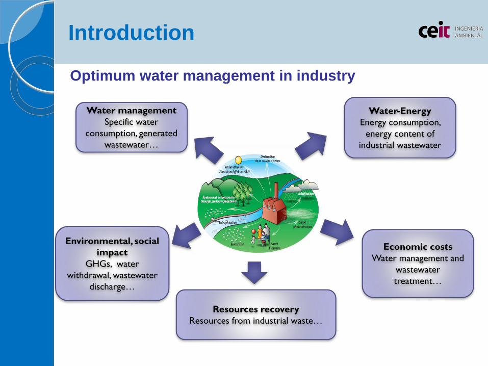
Optimum water management in industry

Introduction

Water management Specific water

consumption, generated wastewater…

Water-Energy Energy consumption,

energy content of industrial wastewater

Economic costs Water management and

wastewater treatment…

Environmental, social impact

GHGs, water withdrawal, wastewater

discharge…

Resources recovery Resources from industrial waste…

Main goal of the project: Development of novel technologies, tools and methodologies for sustainable water management and minimizing water consumption in 4 water consuming industries: paper, textile, food and chemical. CEIT-DHI: development of a simulation tool able to describe water networks in these sectors and obtain optimum solutions (WESTforINDUSTRY)

EU AquafitForUse project

I EU AquafitForUse project

5

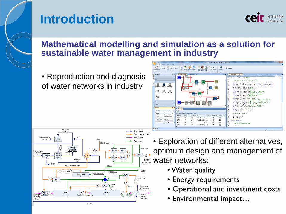
Mathematical modelling and simulation as a solution for sustainable water management in industry

Introduction

• Reproduction and diagnosis of water networks in industry

• Exploration of different alternatives, optimum design and management of water networks:

• Water quality • Energy requirements • Operational and investment costs • Environmental impact…

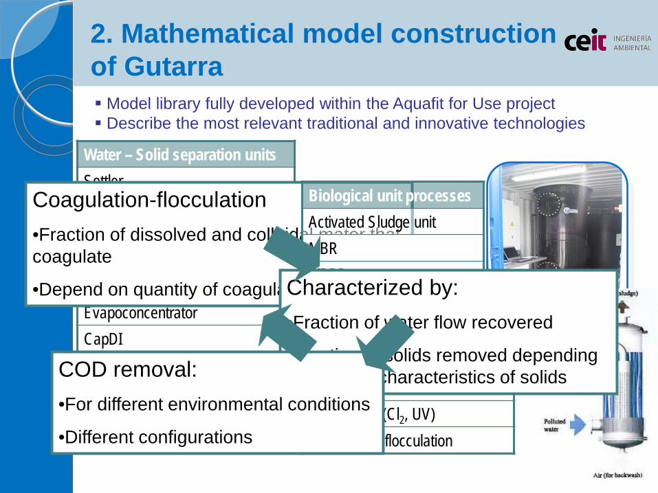
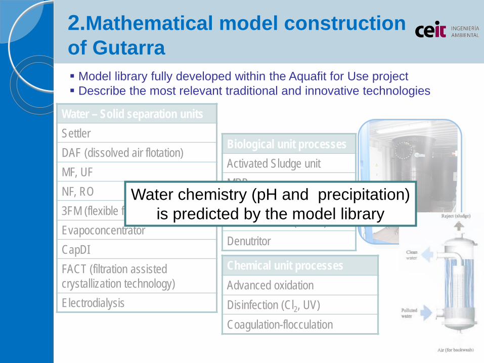
2. Mathematical model construction of Gutarra Model library fully developed within the Aquafit for Use project Describe the most relevant traditional and innovative technologies

Water – Solid separation units Settler DAF (dissolved air flotation) MF, UF NF, RO 3FM (flexible fibre filter module) Evapoconcentrator CapDI FACT (filtration assisted crystallization technology) Electrodialysis

AOP •Inert matter transformed into biodegradable

•Dependent on O3 concentration

Disinfection •Pathogen removal

•Represented by Chick’s law

Coagulation-flocculation •Fraction of dissolved and colloidal mater that coagulate

•Depend on quantity of coagulant added

Chemical unit processes Advanced oxidation Disinfection (Cl2, UV) Coagulation-flocculation

Biological unit processes Activated Sludge unit MBR MBBR Anaerobic unit (UASB) Denutritor

Characterized by: •Fraction of water flow recovered

•Fraction of solids removed depending of physical characteristics of solids COD removal:

•For different environmental conditions

•Different configurations

Model library fully developed within the Aquafit for Use project Describe the most relevant traditional and innovative technologies

Water – Solid separation units Settler DAF (dissolved air flotation) MF, UF NF, RO 3FM (flexible fibre filter module) Evapoconcentrator CapDI FACT (filtration assisted crystallization technology) Electrodialysis

Chemical unit processes Advanced oxidation Disinfection (Cl2, UV) Coagulation-flocculation

Biological unit processes Activated Sludge unit MBR MBBR Anaerobic unit (UASB) Denutritor

Water chemistry (pH and precipitation) is predicted by the model library

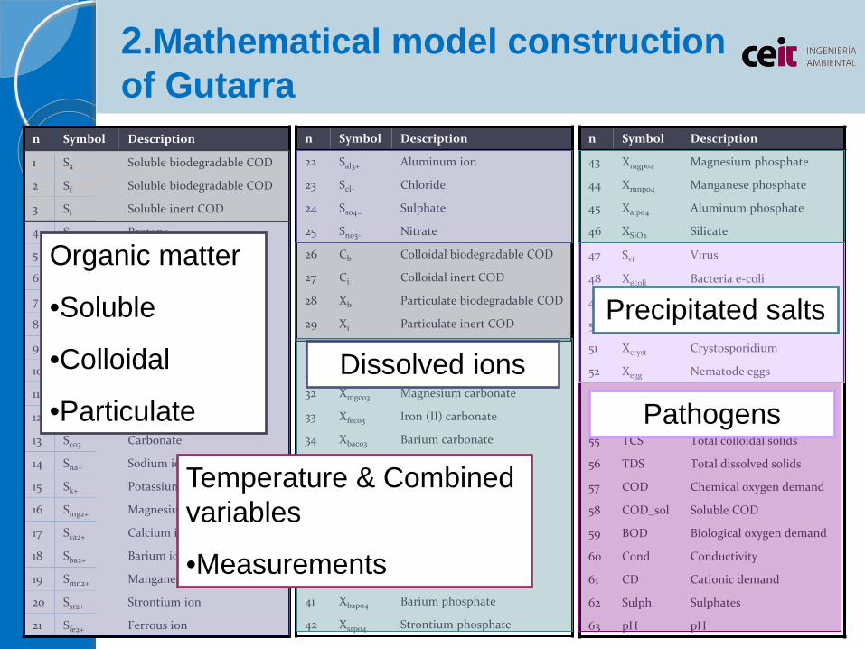
2.Mathematical model construction of Gutarra

n Symbol Description

43 Xmgpo4 Magnesium phosphate

44 Xmnpo4 Manganese phosphate

45 Xalpo4 Aluminum phosphate

46 XSiO2 Silicate

47 Svi Virus

48 Xecoli Bacteria e-coli

49 Xlegionella Legionella

50 Xcyst Cyst-giardia

51 Xcryst Crystosporidium

52 Xegg Nematode eggs

53 Temp Temperature

54 TSS Total suspended solids

55 TCS Total colloidal solids

56 TDS Total dissolved solids

57 COD Chemical oxygen demand

58 COD_sol Soluble COD

59 BOD Biological oxygen demand

60 Cond Conductivity

61 CD Cationic demand

62 Sulph Sulphates

63 pH pH

n Symbol Description

22 Sal3+ Aluminum ion

23 Scl- Chloride

24 Sso4= Sulphate

25 Sno3- Nitrate

26 Cb Colloidal biodegradable COD

27 Ci Colloidal inert COD

28 Xb Particulate biodegradable COD

29 Xi Particulate inert COD

30 Xii Particulate inorganic matter

31 Xcaco3 Calcium carbonate

32 Xmgco3 Magnesium carbonate

33 Xfeco3 Iron (II) carbonate

34 Xbaco3 Barium carbonate

35 Xmnco3 Manganese carbonate

36 Xsrco3 Strontium carbonate

37 Xcaso4 Calcium sulphate

38 Xbaso4 Barium sulphate

39 Xsrso4 Strontium sulphate

40 Xcapo4 Calcium phosphate

41 Xbapo4 Barium phosphate

42 Xsrpo4 Strontium phosphate

n Symbol Description

1 Sa Soluble biodegradable COD

2 Sf Soluble biodegradable COD

3 Si Soluble inert COD

4 Sh Protons

5 Soh Hydroxyl ions

6 Spo4-3 Phosphate

7 Shpo4= Hydroxyl phosphate

8 Sh2po4- Dihydroxyl phosphate

9 Snh4 Ammonium

10 Snh3 Ammonia

11 Sco2 Dissolved carbon dioxide

12 Shco3 Bicarbonate

13 Sco3 Carbonate

14 Sna+ Sodium ion

15 Sk+ Potassium ion

16 Smg2+ Magnesium ion

17 Sca2+ Calcium ion

18 Sba2+ Barium ion

19 Smn2+ Manganese ion

20 Ssr2+ Strontium ion

21 Sfe2+ Ferrous ion

Organic matter

•Soluble

•Colloidal

•Particulate Dissolved ions

Precipitated salts

Pathogens

Temperature & Combined variables

•Measurements

2.Mathematical model construction of Gutarra

• Mass transport – COD biodegradation as function of HRT, SRT (Marais et al., 1976) – Mass transport applied for the following control volumes

ASU Unit MBR Unit MBBR Unit

( )

−= efmax_in

TOT_bulk

HTOT_bulkef,b DOBDOB

fY

·fX

( ) ( )

+−= in,Iefmax_inHHend2

TOT_bulkTOT_bulkef,i XDOBDOBY·b·f·

fHRT·fX

( )efmax_COD_CR_TOT_bulkef,b BOD·f·fC = ( )inf,iR_TOT_bulkef,i CfC =

( ) efmax_COD_Cef,f BOD·f1S −=

COD in effluent

Particulate

Colloidal

Soluble

Models for biological units

• Costs associated with ASU-MBR-MBBR

– Investment cost

– Operational cost

MBBRKinfinf

MBBRMBBR 1000COD·Q·CIC

=

Design parameters from provider

Operational parameters from plant operators (energetic costs)

Models for biological units

OPKinfinf

MBBRMBBR 1000COD·Q·POP

=

Svi Virus

Xecoli

Bacteria e-coli

Xlegionella

Legionella

Xcyst Cyst-giardia

Xcryst

Crystosporidium

Xegg Nematode eggs

UVdoseinDISDIS I·PQ·POP +=

( )in_pathogenout_pathogen X·

100onInactivati100X −

=

inDISDIS Q·CIC =

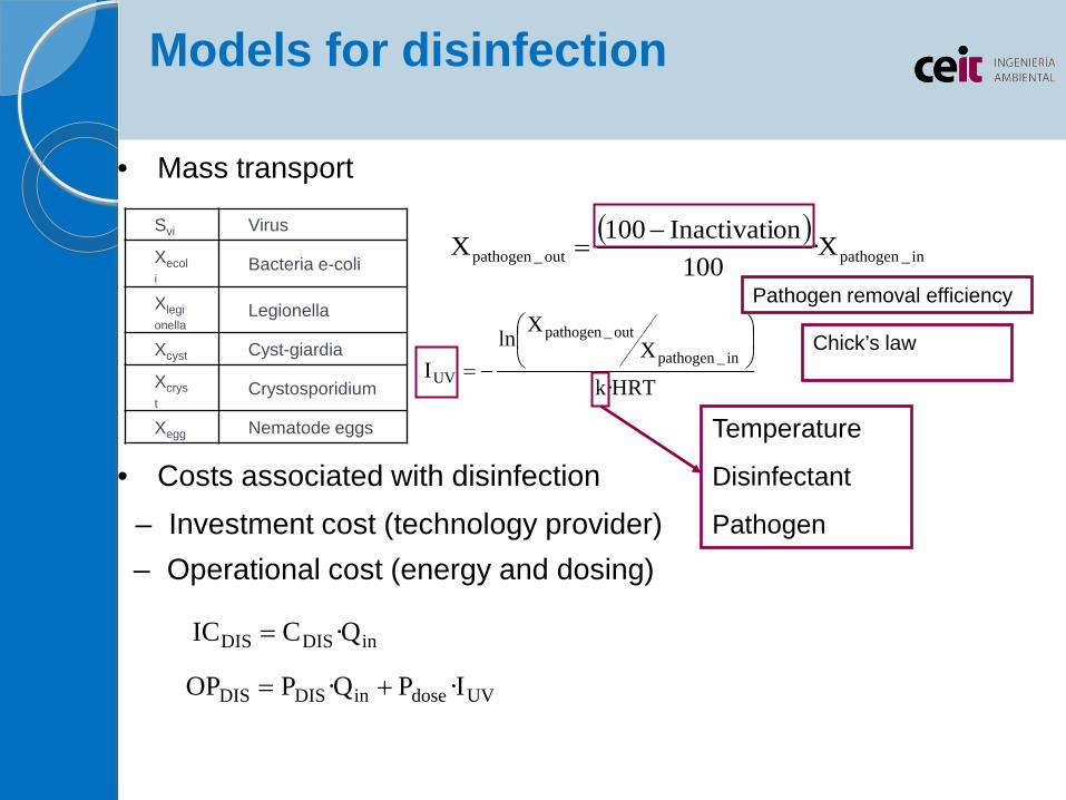
• Mass transport

• Costs associated with disinfection – Investment cost (technology provider) – Operational cost (energy and dosing)

Chick’s law

HRT·k

XXln

I in_pathogen

out_pathogen

UV

−=

Temperature

Disinfectant

Pathogen

Pathogen removal efficiency

Models for disinfection

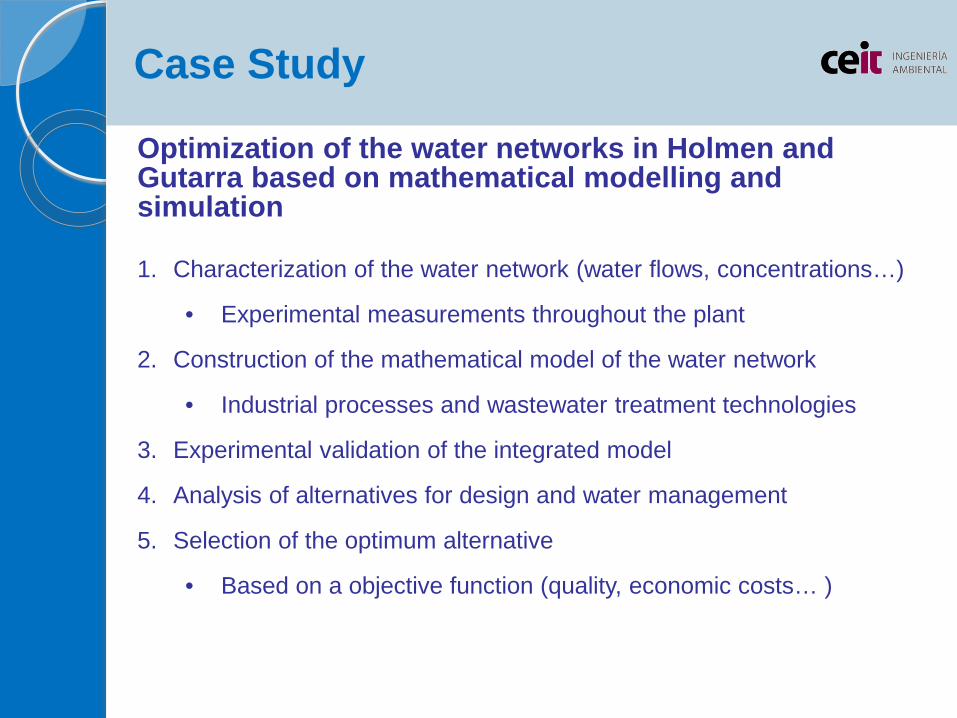
Case Study

Optimization of the water networks in Holmen and Gutarra based on mathematical modelling and simulation

1. Characterization of the water network (water flows, concentrations…)

• Experimental measurements throughout the plant

2. Construction of the mathematical model of the water network

• Industrial processes and wastewater treatment technologies

3. Experimental validation of the integrated model

4. Analysis of alternatives for design and water management

5. Selection of the optimum alternative

• Based on a objective function (quality, economic costs… )

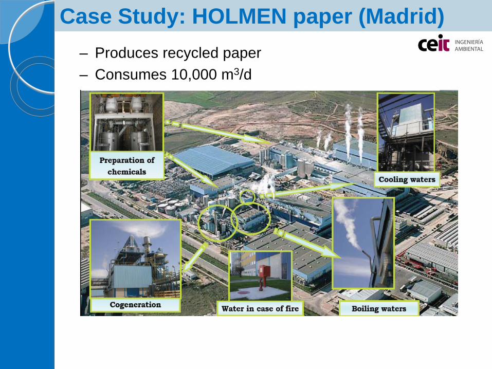
– Produces recycled paper – Consumes 10,000 m3/d

Case Study: HOLMEN paper (Madrid)

Gravity table

Sludge

PM 62

DAF 1

LOOP 1

DAF 2

Product

DAF 3

Cooling tower

Effluent

MBBR3

DAF 4

Evaporation and losses

LOOP 2

Water steam

MBBR1

Cooling processes

MBBR4MBBR2

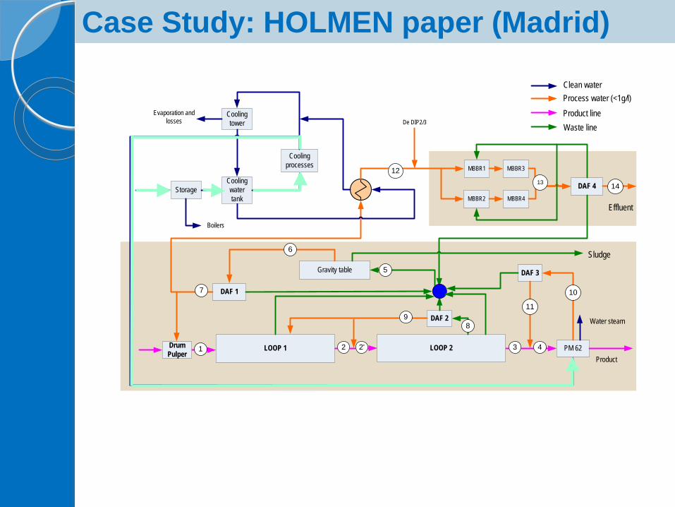
Clean waterProcess water (<1g/l)Product lineWaste line

2 3 4

5

6

7

89

10

11

12

14Storage

Boilers

Cooling water tank

13

De DIP2/3

1Drum Pulper

2'

Case Study: HOLMEN paper (Madrid)

0

5000

10000

15000

20000

25000

30000

35000

40000

45000

1 2 3 4 5 6 7 8 9 10 11 12 13 14

Sampling point

TSS

(g/m

3 )

ExperimentalSimulated

0

100

200

300

400

500

600

700

800

900

1 2 3 4 5 6 7 8 9 10 11 12 13 14

Sampling point

Sulp

hate

s (g

/m3 )

ExperimentalSimulated

0

10

20

30

40

50

60

1 2 3 4 5 6 7 8 9 10 11 12 13 14

Sampling point

Tem

pera

ture

(ºC

)ExperimentalSimulated

0

500

1000

1500

2000

2500

3000

3500

4000

1 2 3 4 5 6 7 8 9 10 11 12 13 14

Sampling point

Solu

ble

CO

D (g

CO

D/m

3 ) ExperimentalSimulated

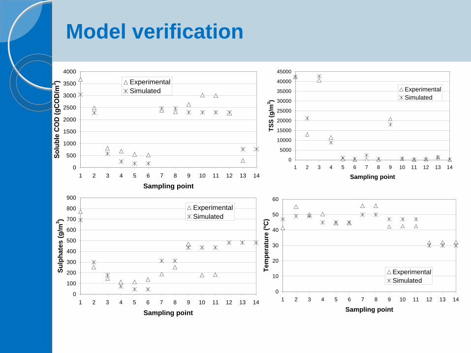
Model verification

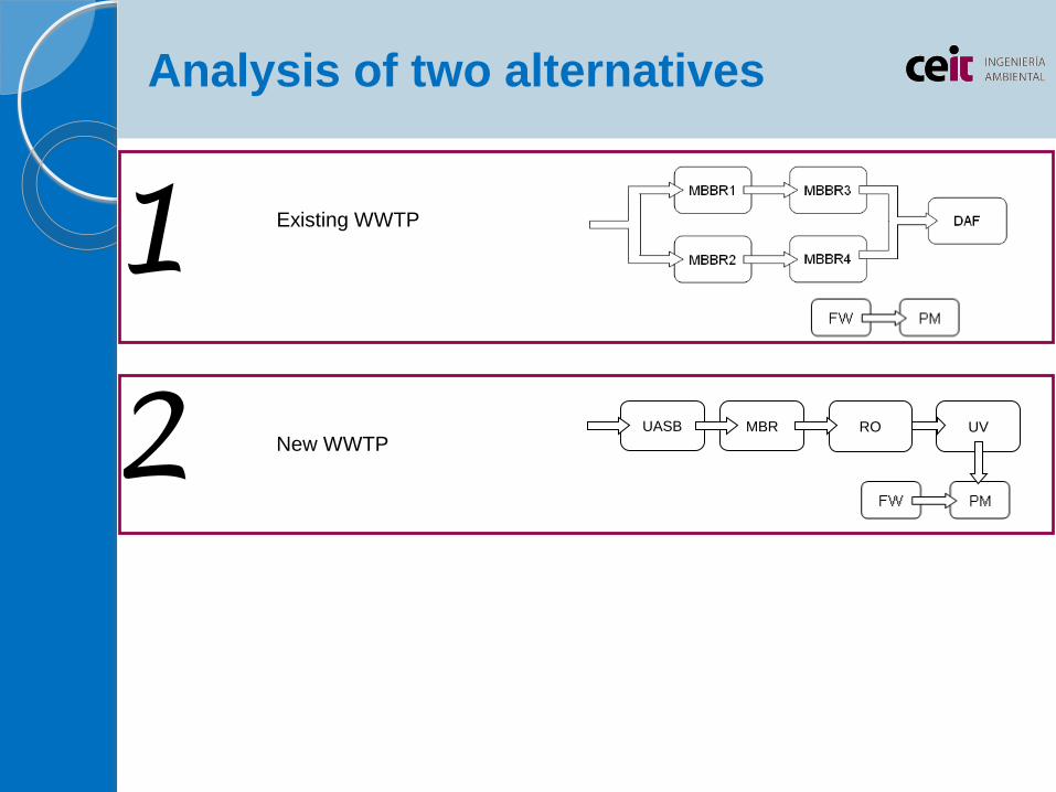
UASB MBR RO UV

Existing WWTP

New WWTP

1

2

Analysis of two alternatives

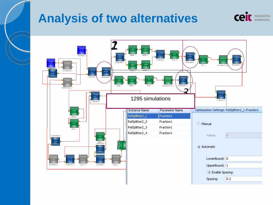
2 1

3

Optimization

1295 simulations

Analysis of two alternatives

( ) N·365·K·Q·411.1N·365·Q·1510

Q·TSS·200N·365·OP

LSN·ICCOST FWw6

ww

treatii

treatnewi ii +

+++

= ∑∑

==

Investment cost

Operational cost

Cost associated with sludge treatment

Drinking water

• Cost function

Analysis of two alternatives

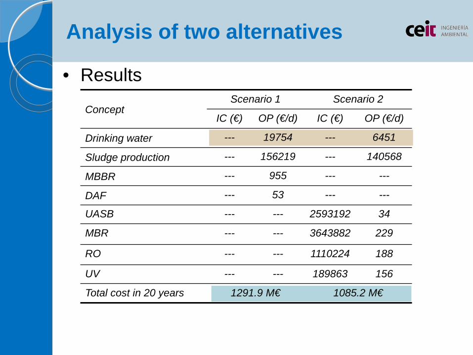
Concept Scenario 1 Scenario 2

IC (€) OP (€/d) IC (€) OP (€/d)

Drinking water --- 19754 --- 6451

Sludge production --- 156219 --- 140568

MBBR --- 955 --- ---

DAF --- 53 --- ---

UASB --- --- 2593192 34

MBR --- --- 3643882 229

RO --- --- 1110224 188

UV --- --- 189863 156

Total cost in 20 years 1291.9 M€ 1085.2 M€

• Results

Analysis of two alternatives

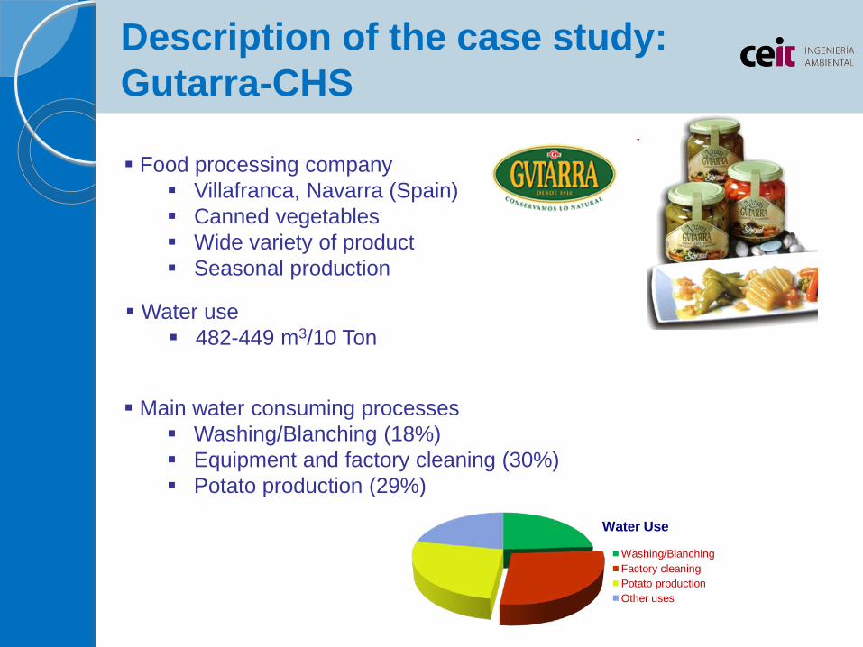
Description of the case study: Gutarra-CHS

Food processing company Villafranca, Navarra (Spain) Canned vegetables Wide variety of product Seasonal production

Main water consuming processes Washing/Blanching (18%) Equipment and factory cleaning (30%) Potato production (29%)

Water Use

Washing/BlanchingFactory cleaningPotato productionOther uses

Water use 482-449 m3/10 Ton

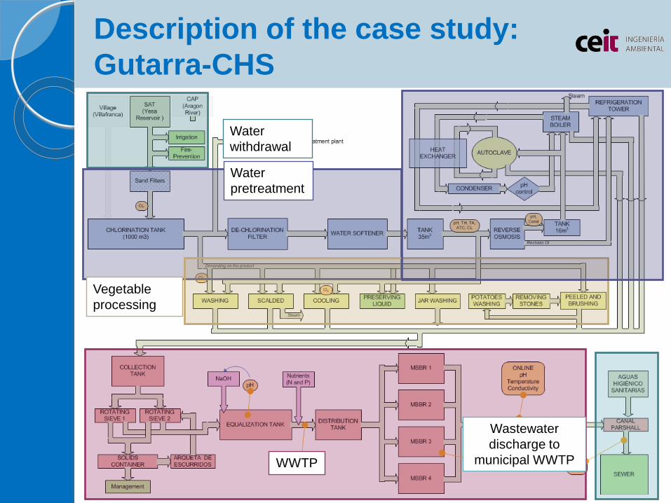
Description of the case study: Gutarra-CHS

Water withdrawal

Water pretreatment

Vegetable processing

WWTP

Wastewater discharge to

municipal WWTP

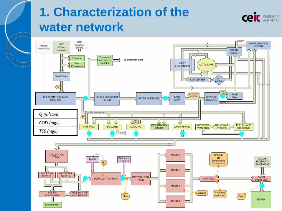
1. Characterization of the water network

Q (m3/ton)

COD (mg/l)

TSS (mg/l)

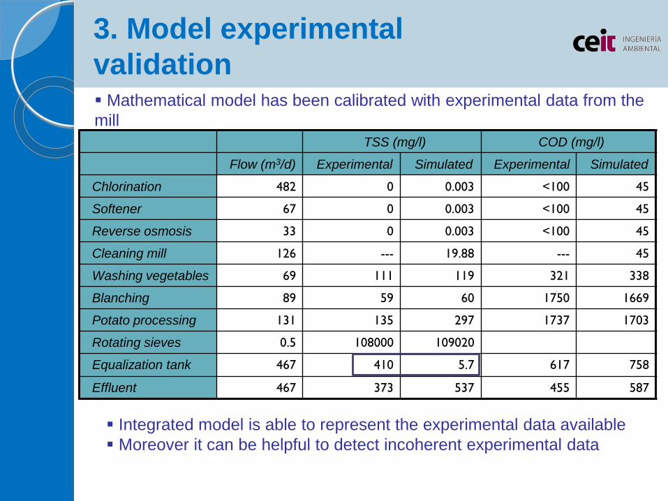
TSS (mg/l) COD (mg/l)

Flow (m3/d) Experimental Simulated Experimental Simulated

Chlorination 482 0 0.003 <100 45

Softener 67 0 0.003 <100 45

Reverse osmosis 33 0 0.003 <100 45

Cleaning mill 126 --- 19.88 --- 45

Washing vegetables 69 111 119 321 338

Blanching 89 59 60 1750 1669

Potato processing 131 135 297 1737 1703

Rotating sieves 0.5 108000 109020

Equalization tank 467 410 5.7 617 758

Effluent 467 373 537 455 587

3. Model experimental validation Mathematical model has been calibrated with experimental data from the mill

Integrated model is able to represent the experimental data available Moreover it can be helpful to detect incoherent experimental data

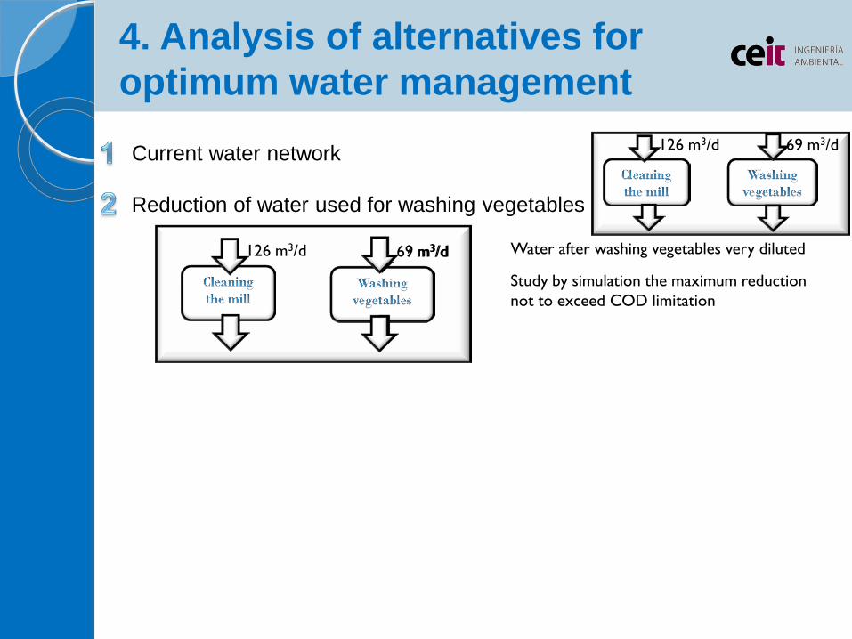
4. Analysis of alternatives for optimum water management

? m3/d 126 m3/d

Current water network

Reduction of water used for washing vegetables

69 m3/d 126 m3/d

69 m3/d Water after washing vegetables very diluted

Study by simulation the maximum reduction not to exceed COD limitation

4. Analysis of alternatives for optimum water management

69 m3/d 57 m3/d

69 m3/d

126 m3/d

? m3/d 126 m3/d

Current water network

Reduction of water used for washing vegetables

Reuse of water from washing vegetables in cleaning the mill

69 m3/d 126 m3/d

126 m3/d

69 m3/d Water after washing vegetables very diluted

Study by simulation the maximum reduction not to exceed COD limitation

Study the possibility of reusing water from vegetable washing in cleaning the mill after some treatment

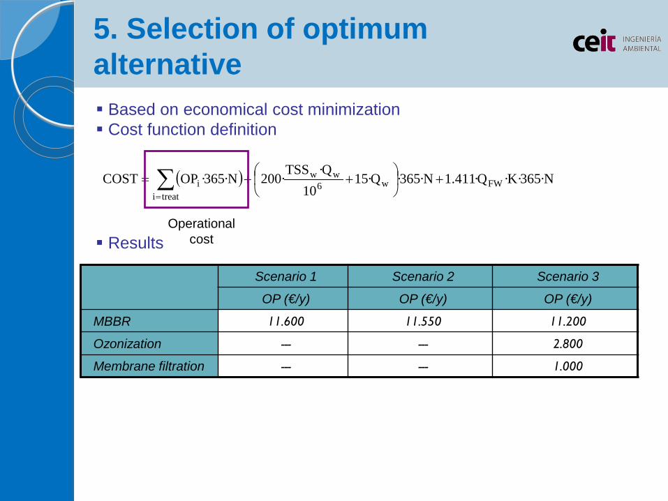
Based on economical cost minimization Cost function definition

Results

( ) N·365·K·Q·411.1N·365·Q·1510

Q·TSS·200N·365·OPCOST FWw6

ww

treatii +

++= ∑=

Scenario 1 Scenario 2 Scenario 3

OP (€/y) OP (€/y) OP (€/y)

MBBR 11.600 11.550 11.200

Ozonization --- --- 2.800

Membrane filtration --- --- 1.000

Operational cost

5. Selection of optimum alternative

Based on economical cost minimization Cost function definition

Results

( ) N·365·K·Q·411.1N·365·Q·1510

Q·TSS·200N·365·OPCOST FWw6

ww

treatii +

++= ∑=

Sludge treatment

Scenario 1 Scenario 2 Scenario 3

OP (€/y) OP (€/y) OP (€/y)

MBBR 11.600 11.550 11.200

Ozonization --- --- 2.800

Membrane filtration --- --- 1.000

Scenario 1 Scenario 2 Scenario 3

OP (€/y) OP (€/y) OP (€/y)

MBBR 11.600 11.550 11.200

Ozonization --- --- 2.800

Membrane filtration --- --- 1.000

Sludge production 6.600 6.000 5.200

5. Selection of optimum alternative

Based on economical cost minimization Cost function definition

Results

( ) N·365·K·Q·411.1N·365·Q·1510

Q·TSS·200N·365·OPCOST FWw6

ww

treatii +

++= ∑=

Fresh water

Scenario 1 Scenario 2 Scenario 3

OP (€/y) OP (€/y) OP (€/y)

MBBR 11.600 11.550 11.200

Ozonization --- --- 2.800

Membrane filtration --- --- 1.000

Sludge production 6.600 6.000 5.200

Scenario 1 Scenario 2 Scenario 3

OP (€/y) OP (€/y) OP (€/y)

MBBR 11.600 11.550 11.200

Ozonization --- --- 2.800

Membrane filtration --- --- 1.000

Sludge production 6.600 6.000 5.200

Drinking water 240.000 228.000 220.000

5. Selection of optimum alternative

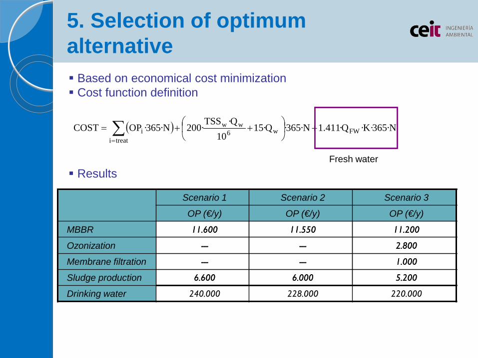
Based on economical cost minimization Cost function definition

Results

( ) N·365·K·Q·411.1N·365·Q·1510

Q·TSS·200N·365·OPCOST FWw6

ww

treatii +

++= ∑=

Scenario 1 Scenario 2 Scenario 3

OP (€/y) OP (€/y) OP (€/y)

MBBR 11.600 11.550 11.200

Ozonization --- --- 2.800

Membrane filtration --- --- 1.000

Sludge production 6.600 6.000 5.200

Drinking water 240.000 228.000 220.000

Total cost (€/y) 258.200 €/y 245.550 €/y 240.200 €/y

-5% -8%

5. Selection of optimum alternative

Conclusions

• Mathematical modelling and simulation are shown to be valuable tools for design and seeking optimum water management solutions

• The mathematical model constucted has enabled to:

• Describe the water network present in Holmen and Gutarra in a realistic way

• Propose new water management solutions that minimize water consumption and consecuently minimize operational costs

Simulation tool for optimum water management in industry

Paloma Grau Girona, 7th February, 2014