Simulations of Ground Motion in the Los Angeles Basin...

187

Bulletin of the Seismological Society of America, Vol. 94, No. 1, pp. 187–206, February 2004

Simulations of Ground Motion in the Los Angeles Basin Based

upon the Spectral-Element Method

by Dimitri Komatitsch, Qinya Liu, Jeroen Tromp, Peter Suss,* Christiane Stidham,and John H. Shaw

Abstract We use the spectral-element method to simulate ground motion gener-ated by two recent and well-recorded small earthquakes in the Los Angeles basin.Simulations are performed using a new sedimentary basin model that is constrainedby hundreds of petroleum-industry well logs and more than 20,000 km of seismicreflection profiles. The numerical simulations account for 3D variations of seismic-wave speeds and density, topography and bathymetry, and attenuation. Simulationsfor the 9 September 2001 Mw 4.2 Hollywood earthquake and the 3 September 2002Mw 4.2 Yorba Linda earthquake demonstrate that the combination of a detailed sed-imentary basin model and an accurate numerical technique facilitates the simulationof ground motion at periods of 2 sec and longer inside the basin model and 6 secand longer in the regional model. Peak ground displacement, velocity, and acceler-ation maps illustrate that significant amplification occurs in the basin.

Introduction

Accurate prediction of hazardous ground shaking gen-erated by large earthquakes requires the ability to numeri-cally simulate seismic-wave propagation in realistic geolog-ical models. In this article we demonstrate that, using adetailed model of the Los Angeles, California, basin (Fig. 1)and an accurate numerical technique, ground motion can beaccurately modeled down to a period of 2 sec inside the basinmodel and 6 sec in the regional model.

The Los Angeles basin developed in the Neogene as aresult of regional crustal extension associated with the open-ing of the California Borderlands and rotation of the Trans-verse Ranges (Luyendyk and Hornafius, 1987; Wright,1991). Since the early Pliocene, the basin has been deformedby numerous strike-slip, reverse, and blind-thrust faults thataccommodate oblique convergence between the Pacific andNorth American plates (e.g., Davis et al., 1989; Hauksson,1990; Wright, 1991; Schneider et al., 1996; Shaw andSuppe, 1996; Shaw and Shearer, 1999; Fuis et al., 2003).This tectonic history, combined with varied depositional anddiagenetic processes involving the basin sediments, hasyielded complex 3D wave-speed and density structures inthe Los Angeles basin (e.g., Suss and Shaw, 2003).

Regional studies initially focused on developing aver-age 1D models (e.g., Hadley and Kanamori, 1977; Dregerand Helmberger, 1990). Three-component broadband re-cords of small earthquakes were used in Dreger and Helm-

*Now at Institut fur Geologie und Palaontologie, University of Tubingen,Sigwartstrasse 10, 72076 Tubingen, Germany.

berger (1990) to study the sensitivity of synthetic seismo-grams to perturbations of the crustal model and to constructan average 1D layered model of crustal structure. More re-cently, taking advantage of the large number of broadbandseismic stations and the related wealth of high-quality data,regional tomographic Vp and Vp/Vs models have been con-structed (e.g., Hauksson and Haase, 1997; Hauksson, 2000)based upon P and S-P travel times from local earthquakesand controlled artificial sources. The 3D shape of the south-ern California Moho has also been imaged (e.g., Ichinose etal., 1996; Lewis et al., 2000; Zhu and Kanamori, 2000).Based upon the teleseismic receiver function technique, Zhuand Kanamori (2000) have shown that very significant var-iations of Moho depth exist in the region, from 21 to 37 km,with a regional average of 29 km. A deep Moho is foundunder the eastern Transverse Range, the Peninsular Range,and the Sierra Nevada Range. To the contrary, the centralTransverse Range does not have a deep continental root. Thecrust is much thinner (typically 21–22 km) in the Inner Cali-fornia Borderland and the Salton Trough. In the past fewyears, the Southern California Earthquake Center (SCEC)has focused on creating 3D wave-speed models of the region(e.g., Magistrale et al., 1996, 2000; Graves, 1999). TheSCEC model is a rule-based wave-speed description, cali-brated with seven sonic logs, that relates Vp to the age anddepth of strata. In contrast, the model we use for our simu-lations is interpolated from more than 150 sonic logs and7000 stacking velocities derived from petroleum-industry re-flection profiles (Suss and Shaw, 2003). The two models

188 D. Komatitsch, Q. Liu, J. Tromp, P. Suss, C. Stidham, and J. H. Shaw

121˚W 120˚W 119˚W 118˚W 117˚W 116˚W 115˚W 114˚W

32˚N

33˚N

34˚N

35˚N

36˚N

37˚N

Coast Ranges

Transverse Ranges

Great Valley

Sierra N

evada

Death Valley

Peninsular Ranges

Continental Borderland

Mojave Desert

BajaCalifornia

San Andreas Fault

Garlock Fault

Imperial

Valley Fault

San Jacinto Fault

Elsinore Fault

Ventura Basin

LA Basin

San Gabriel Mtns San Bernardino Mtns

EC

SZ

San Fernando

Palos Verdes

Salton Sea

Figure 1. Topographic map of southernCalifornia showing the Los Angeles region.The small California map in the lower left-hand corner shows the location of the area rep-resented (red rectangle). The main late Quater-nary faults (Jennings, 1975) are also displayed.ECSZ, Eastern California Shear Zone. TriNetstations are indicated by white triangles. Thelarge blue rectangle shows the edges of thecomputer grid that we use to perform our 3Dground-motion calculations. The two smallerblue rectangles are the edges of the medium-and high-resolution Los Angeles basin models,respectively. The epicenters of the Hollywoodand Yorba Linda earthquakes studied in thisarticle are denoted by red stars.

have similar average velocity functions, but our model de-scribes more detailed lateral and vertical wave-speed struc-ture that is observed in borehole and stacking velocity data.

Accurate numerical techniques are needed in order tounderstand ground motion in complex 3D structures and tostudy past large earthquakes or hypothetical earthquake sce-narios and their impact in terms of seismic hazard, buildingcodes, disaster prevention, and emergency planning. Nu-merical simulations of ground motion in complex hetero-geneous structures have previously been performed basedupon techniques that can handle highly heterogeneous 3Dmodels, such as the finite-difference (e.g., Boore, 1972;Frankel and Leith, 1992; Frankel and Vidale, 1992; Mc-Laughlin and Day, 1994; Olsen et al., 1995; Pitarka andIrikura, 1996a; Antolik et al., 1996; Larsen et al., 1997; Kris-tek et al., 1999; Stidham et al., 1999; Ji et al., 2000; Satohet al., 2001) and finite-element methods (e.g., Lysmer andDrake, 1972; Bao et al., 1998; Bielak et al., 1999; Garataniet al., 2000; Aagaard et al., 2001).

Several studies have focused more specifically on south-ern California and the Los Angeles basin (e.g., Frankel,1993; Olsen and Archuleta, 1996; Pitarka and Irikura,1996b; Olsen et al., 1997; Wald and Graves, 1998; Graves,1999; Olsen, 2000; Peyrat et al., 2001; Eisner and Clayton,2002). The complexity of the seismic response of the LosAngeles basin has been analyzed by many authors in recentyears, for example, Hartzell et al. (1996, 1998), Wald andGraves (1998), and Olsen (2000). Detailed reviews are avail-able in particular in Wald and Graves (1998) and Olsen(2000). There is evidence that large amplification (factors of3, 4, or more) can occur between basin sites and hard-rocksites. It has also been shown that site effects caused by to-

pography or local geological features, such as poorly con-solidated sediments, can result in very significant amplifi-cation of the wave field (e.g., Gaffet and Bouchon, 1989;Frankel and Leith, 1992; Stevens et al., 1993). Such phe-nomena have been observed in the Los Angeles region, forexample, very large accelerations (up to 1.8g) at TarzanaHill during the 1994 Northridge earthquake (e.g., Bouchonand Barker, 1996; Catchings and Lee, 1996; Rial, 1996; Spu-dich et al., 1996; Komatitsch and Vilotte, 1998). Localiza-tion effects can also cause important damage, as illustratedin Santa Monica during the 1994 Northridge earthquake(e.g., Gao et al., 1996; Alex and Olsen, 1998; Davis et al.,2000). Such effects are intrinsically 3D and therefore furtherillustrate the need for detailed basin models and accurate andflexible numerical techniques.

In this article, we present simulations based on a de-tailed model of the Los Angeles basin (Suss and Shaw, 2003)and a powerful numerical technique called the spectral-element method (SEM). Using two recent well-recordedsmall (Mw 4.2) earthquakes in the basin, we show thatground motion can be accurately modeled down to a periodof 2 sec inside the basin model and 6 sec in the regionalmodel. The SEM has several distinct advantages over moreclassical numerical techniques mentioned earlier, as will beillustrated in the Numerical Technique section.

Basin Model

Creating a high-resolution wave-speed model of the LosAngeles basin (Fig. 1) has been the focus of significant at-tention in recent years. Collaborative efforts in the contextof the SCEC have led to the development of models that are

Simulations of Ground Motion in the Los Angeles Basin Based upon the Spectral-Element Method 189

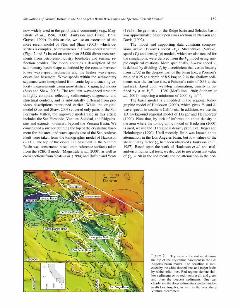
Figure 2. Top view of the surface definingthe top of the crystalline basement in the LosAngeles basin model. The coastline is indi-cated by the white dashed line, and major faultsby white solid lines. Red regions denote shal-low sediments or no sediments at all, and greenand blue the deepest sediments. One canclearly see the deep sedimentary pocket under-neath Los Angeles, as well as the very sharpVentura escarpment.

now widely used in the geophysical community (e.g., Mag-istrale et al., 1996, 2000; Hauksson and Haase, 1997;Graves, 1999). In this article, we use an extension of themore recent model of Suss and Shaw (2003), which de-scribes a complex, heterogeneous 3D wave-speed structure(Figs. 2 and 3) based on more than 85,000 direct measure-ments from petroleum-industry boreholes and seismic re-flection profiles. The model contains a description of thesedimentary basin shape as defined by the contact betweenlower wave-speed sediments and the higher wave-speedcrystalline basement. Wave speeds within the sedimentarysequence were interpolated from sonic log and stacking ve-locity measurements using geostatistical kriging techniques(Suss and Shaw, 2003). The resultant wave-speed structureis highly complex, reflecting sedimentary, diagenetic, andstructural controls, and is substantially different from pre-vious descriptions mentioned earlier. While the originalmodel (Suss and Shaw, 2003) covered only parts of the SanFernando Valley, the improved model used in this articleincludes the San Fernando, Ventura, Soledad, and Ridge ba-sins and extends northward beyond the Ventura Basin. Weconstructed a surface defining the top of the crystalline base-ment for this area, and wave speeds east of the San AndreasFault were taken from the tomographic model of Hauksson(2000). The top of the crystalline basement in the VenturaBasin was constructed based upon reference surfaces takenfrom the SCEC-II model (Magistrale et al., 2000), as well ascross sections from Yeats et al. (1994) and Huftile and Yeats

(1995). The geometry of the Ridge basin and Soledad basinwas approximated based upon cross sections in Namson andDavis (1992).

The model and supporting data constrain compres-sional-wave (P-wave) speed (Vp). Shear-wave (S-wave)speed (Vs) and density (q) models, which are also needed forthe simulations, were derived from the Vp model using sim-ple empirical relations. More specifically, S-wave speed Vs

is defined by dividing Vp by a coefficient that varies linearlyfrom 1.732 in the deepest part of the basin (i.e., a Poisson’sratio of 0.25 at a depth of 8.5 km) to 2 in the shallow sedi-ments near the surface (i.e., a Poisson’s ratio of 0.33 at thesurface). Based upon well-log information, density is de-fined by q � Vp/3 � 1280 (McCulloh, 1960; Stidham etal., 2001), imposing a minimum of 2000 kg m�3.

The basin model is embedded in the regional tomo-graphic model of Hauksson (2000), which gives P- and S-wave speeds in southern California. In addition, we use the1D background regional model of Dreger and Helmberger(1990). Note that, by lack of information about density inthe area where the tomographic model of Hauksson (2000)is used, we use the 1D regional density profile of Dreger andHelmberger (1990). Until recently, little was known aboutattenuation in the Los Angeles basin, but low values of theshear quality factor Ql had been observed (Hauksson et al.,1987). Based upon the work of Hauksson et al. and trial-and-error numerical tests, we decided to use a constant valueof Ql � 90 in the sediments and no attenuation in the bed-


rock. It would ultimately be of interest to use the recentattenuation scaling rules of Olsen et al. (2003). Lateral var-iations in crustal thickness are incorporated based upon theregional Moho model of Zhu and Kanamori (2000). Topog-raphy and bathymetry are obtained from a U.S. GeologicalSurvey (USGS) digital elevation map (USGS, 2003), as il-lustrated in Figure 3.

Numerical Technique

We use the SEM to simulate ground motion in the basin,based upon the linear anelastic wave equation. Nonlinear

effects are not taken into account in this article. The SEM isa highly accurate numerical method that has its origins incomputational fluid dynamics (Patera, 1984). It uses a meshof hexahedral finite elements on which the wave field is rep-resented in terms of high-degree Lagrange polynomials onGauss–Lobatto–Legendre interpolation points. The methodwas used to model seismic-wave propagation in local andregional models in the 1990s (e.g., Cohen et al., 1993; Prioloet al., 1994; Faccioli et al., 1997; Komatitsch, 1997; Ko-matitsch and Vilotte, 1998; Komatitsch and Tromp, 1999).It was more recently introduced for global wave propagationby Chaljub (2000) and extended for large-scale global wavepropagation (Komatitsch and Tromp, 2002a,b; Capdeville etal., 2003; Chaljub et al., 2003).

The main advantage of the SEM is that it combines theflexibility of the finite-element method (e.g., Lysmer andDrake, 1972; Moczo et al., 1997; Bao et al., 1998; Bielaket al., 1999; Garatani et al., 2000) with the accuracy of pseu-dospectral techniques (e.g., Tessmer et al., 1992; Carcioneand Wang, 1993; Igel, 1999). It is more accurate than widelyused classical techniques such as the finite-differencemethod (e.g., Boore, 1972; Virieux, 1986; Graves, 1996;Olsen et al., 1997), in particular for surface waves (e.g.,Komatitsch and Tromp, 1999, 2002a), which play an im-portant role in ground-motion seismology.

In the SEM, it is relatively straightforward to densify themesh near the surface of the model in the low wave-speedsediments, using mesh doubling as a function of depth, asillustrated in Figure 4, assuming that the surfaces do notexhibit large local variations (i.e., that they are smoothenough). Using a coarser mesh in depth significantly reducesthe memory requirements and facilitates an increase in thevalue of the time step, thus enabling larger simulations fora similar computational cost. Due to the geometrical flexi-bility that the SEM shares with the finite-element method,the mesh can be adapted to topography and bathymetry aswell as the shape of the basement surface and the Moho (Fig.4). Even in the presence of substantial topography, the trac-tion-free boundary condition at the Earth’s free surface issatisfied automatically in a SEM (e.g., Komatitsch and Vil-otte, 1998; Komatitsch and Tromp, 1999, 2002a).

The choice of high-degree Lagrange polynomial inter-polants combined with Gauss–Lobatto–Legendre quadratureresults in minimal numerical grid dispersion. Because of thisparticular choice of integration points and numerical inte-gration rule, the SEM’s most important property is an exactlydiagonal mass matrix, which leads to a simple explicit timeintegration scheme without needing to solve a system of lin-ear equations (e.g., Komatitsch and Vilotte, 1998; Koma-titsch and Tromp, 1999, 2002a). Because of the fact that themass matrix is exactly diagonal, another property of the SEMis that it is very well adapted to the parallel distributed mem-ory architecture of modern computers (Komatitsch andTromp, 2001; Komatitsch et al., 2003), an advantage itshares with the finite-difference method. This implies thatthe SEM is simpler to implement than traditional finite-element methods.

Figure 3. View from the southeast upon the LosAngeles basin model. (a) North–south and east–westcross sections showing P-wave speed in the basinmodel, with blue denoting fast bedrock and white andred slower deep and shallow sediments, respectively.The coastline is shown by the white line. The maxi-mum depth of the basin is 8.5 km underneath down-town Los Angeles. The basin model is embedded intothe regional tomographic model of Hauksson (2000)(not shown here). (b) Surface topography and ba-thymetry. One can clearly see the San Gabriel moun-tains toward the north, Palos Verdes along the coast,as well as the Ventura, San Fernando, and Los An-geles basins.


Figure 4. North–south cross section through themesh of the Los Angeles basin region. For clarity,only the vertical edges of the mesh slices are repre-sented. The blue line shows the Mexican border, thecoastline, Palos Verdes, and Santa Catalina Island.The mesh is adapted to the deepest part of the base-ment surface and to the shape of the Moho taken fromZhu and Kanamori (2000). It is doubled in size twice:first below the low wave-speed surface layer and asecond time below the basement. Red represents ele-ments located below the Moho, green elements be-tween the Moho and the bottom of the sedimentarypocket, and yellow elements in the upper part of themodel honoring the shape of the surface and the bot-tom of the sedimentary pocket. Note that for geo-metrical reasons, we only honor the bottom part ofthe deep sedimentary pocket (from a depth of 4 kmto a maximum of 8.5 km), otherwise we would beunable to mesh the entire structure in regions withvery thin (or without) sediments.

In this article, we incorporate 3D variations in P- andS-wave speeds, density, and attenuation. The mesh covers516 km � 507 km, from 120.3� W to 114.7� W and from32.2� N to 36.8� N, incorporates most of the roughly 140broadband seismographic stations in the TriNet network(www.trinet.org) in southern California, and extends to adepth of 60 km. It is important to honor the major discon-tinuities in the wave-speed model when creating a mesh ofthe structure, to avoid numerical diffraction by a staircasediscretization of the complex-shaped interfaces (e.g., Zah-radnık et al., 1993). Therefore, the basin mesh honors theshape of the Moho (Zhu and Kanamori, 2000), the lowerpart of the sedimentary basin underneath Los Angeles (Sussand Shaw, 2003), as well as topography and bathymetry(USGS, 2003), as illustrated in Figure 4.

In the TriNet network, there are several seismographicstations on the offshore Channel Islands; for this reason theeffect of the oceanic water layer is incorporated in the mod-

eling based upon an equivalent load formulation that takesinto account the weight of the water column (Komatitschand Tromp, 2002b). This is a long-period approximation thatis valid as long as the wavelength of the seismic signals islarge compared to the depth of the oceans. The main limi-tations of such an approximation are discussed in Koma-titsch and Tromp (2002b). In the case of the Los Angelesregion, we perform simulations at minimum periods of 2 sec,that is, the wavelength in the oceans is 2 � 1500 � 3000 m,which means that the approximation is valid for shallowoceans, typically with a maximum depth of 500–600 m. For-tunately, this is the case in most parts of the model, as illus-trated in Figure 3. Paraxial absorbing conditions (Claytonand Engquist, 1977) are used on the vertical edges and thebottom of the grid to simulate a semi-infinite regional me-dium. More accurate absorbing boundary conditions, suchas the perfectly matched layer (e.g., Berenger, 1994; Chewand Liu, 1996; Collino and Tsogka, 2001; Komatitsch andTromp, 2003), could be used instead, but, because we use alarge mesh, the simpler paraxial conditions are sufficient.

The method is implemented on a PC cluster computer,a so-called Beowulf machine, using parallel programmingbased upon a message-passing technique, making use of themessage-passing interface (Gropp et al., 1996). To take ad-vantage of the parallel machine architecture, the mesh is di-vided into 144 slices that are distributed over 144 processorsusing a regular mesh partitioning topology. The mesh con-tains 672,768 spectral elements. We use a polynomial degreeN � 4 to sample the wave field; therefore each spectralelement contains (N � 1)3 � 125 Gauss–Lobatto–Legendrepoints. Counting points on common spectral-element edgesand corners only once, the mesh therefore contains a totalof 45.4 million grid points (i.e., 136 million degrees of free-dom, because we solve for the three components of displace-ment at each grid point). The average distance between gridpoints at the surface is roughly 335 m. One needs to useroughly five points per wavelength to correctly sample thewave field in the SEM (e.g., Seriani and Priolo, 1994); there-fore the mesh resolves waves with a shortest period of about2 sec. The calculations require 14 Gb of distributed memory.On our cluster it takes about 6.5 hr to compute seismogramswith a duration of 3 min. We use a timestep of 9 msec, thatis, a total of 20,000 timesteps.

Validation for a One-Dimensional Model

In previous work, we carefully benchmarked the SEMagainst semianalytical solutions for reference Earth modelswith and without attenuation (Komatitsch and Vilotte, 1998;Komatitsch and Tromp, 1999; Komatitsch et al., 1999; Ko-matitsch and Tromp, 2002a) and showed its accuracy formodeling seismic-wave propagation. To demonstrate thatthe nonstructured mesh represented in Figure 4 is efficientfor basin models, we study a simple structure consisting ofan anelastic layer over a half-space. We use the model shownin Figure 5, which is known as the SCEC/PEER (Pacific


p s µρV = 4000 V = 2000 = 2600 Q = 40

p s µρV = 6000 V = 3464 = 2700 Q = 69.3

Free surface

30 km

30 km

17 km

1 km

0 km

Figure 5. 1D structure used to assess the accuracyof the SEM for an average basin model. The 3D modelconsists of a layer over a half-space. The horizontalsize of the block is 30 km � 30 km, and it extendsto a depth of 17 km. This reference model is knownas the SCEC/PEER LOH-3 benchmark.

Figure 6. Traces recorded at the surface for theaverage 1D basin model shown in Figure 5. Thesource is a point dislocation located in the half-spacebelow the sedimentary layer in the middle of the blockat a depth of 2 km. The receiver is located at a hori-zontal distance of 10 km from the source. The vertical(top), radial (middle), and transverse (bottom) com-ponents of velocity computed using the SEM (dashedline) are compared to the solution computed basedupon a modified frequency–wavenumber method(Apsel and Luco [1983], solid line). The two curvesare almost perfectly superimposed, which illustratesthe accuracy of the SEM, including for surface waves.

Earthquake Engineering Research Center) LOH-3 bench-mark (peer.berkeley.edu). The block has a horizontal size of30 km � 30 km and extends to a depth of 17 km. Absorbingconditions are used on all sides of the model except the freesurface, in order to simulate a semi-infinite medium. Mate-rial properties in the half-space are Vp � 6000 m s�1, Vs �3464 m s�1, q � 2700 kg m�3, and a shear quality factorQl � 69.3 for attenuation. In the layer, Vp � 4000 m s�1,Vs � 2000 m s�1, q � 2600 kg m�3, and Ql � 40. Theshear quality factor does not depend on frequency (i.e., theattenuation spectrum is flat). The bulk quality factor Qj isinfinite in both regions. Wave speeds Vp and Vs are for areference frequency of 2.5 Hz. The source is a point dislo-cation located in the half-space below the layer in the middleof the grid, at a depth of 2 km. The only nonzero componentof the moment tensor is Mxy � 1018 N m. The moment-ratetime variation of the source is (t/T2) exp(�t/T), where T �0.05 sec. The timestep is Dt � 3.25 msec, and we propagatethe signal for 10 sec. A receiver is placed at x � 6 km andy � 8 km, at a horizontal distance of 10 km from the source,and records the three components of velocity. In Figure 6,we show the results and compare them to a frequency–wave-number reference solution computed based on a modifiedversion of Apsel and Luco (1983). The two results are almostperfectly superimposed, which allows us to conclude thatthe method is very accurate for such an average 1D basinmodel.

Simulations of the 9 September 2001 MW 4.2Hollywood Earthquake

To assess the quality of the 3D basin model and the 3DSEM simulations, we simulated ground motion for the 9 Sep-tember 2001 Mw 4.2 Hollywood earthquake. This event was

located right inside the basin at a depth of approximately4.5 km and was well recorded by TriNet; it therefore pro-vides an excellent test of the 3D basin model and the nu-merical method. Complications associated with source com-plexity and directivity for larger events (e.g., Wald et al.,1996; Ji et al., 2002) are avoided. To obtain the source mech-anism for this event, we performed a 3D centroid moment


tensor (CMT) inversion based upon the basin model and theSEM. We calculated the required 3D Frechet derivatives nu-merically (Liu et al., 2002) by minimizing the waveformmisfit between data and synthetic seismograms to obtain thebest estimated source parameters. The solution is in excellentagreement with first-motion and surface-wave estimates.

Figure 7 shows snapshots of the simulation. The verticalcomponent of velocity at the surface is represented. If thebasin model were 1D, one would see concentric circles cen-tered on the epicenter. The highly distorted wave fronts aredue to substantial 3D variations in the model. Note that en-ergy gets trapped in the Los Angeles and San Fernando ba-sins due to the low wave-speed sediments. This is particu-larly clear between 63.8 and 85.4 sec, where ground motionlasts much longer in the basin than in the surrounding moun-tains and in the Palos Verdes peninsula.

In Figure 8 we compare the results of 3D SEM simula-tions to three-component displacement data recorded byTriNet stations. Both data and synthetic seismograms arebandpass filtered between 6 and 35 sec with a four-pole two-pass Butterworth filter. We focus our attention on the LosAngeles region, where the detailed Harvard basin model isdefined and in which the event took place. Notice that atthese periods we can fit the data very well on all three com-ponents. The model captures the amplifications and reso-nance associated with the Los Angeles basin, for example,transverse components at LAF, STS, LGB, and PDR andradial components are PDR, WTT, and LLS. Notice thatstations in the San Gabriel mountains (e.g., CHF, BFS, TA2,and MWC) have relatively small displacements on all threecomponents that are well fit by the synthetic seismograms.The good fit to the data demonstrates that the SEM wavefrontdistortions in Figure 7 capture actual facets of the data. Be-cause the model is a P-wave speed model and the largestsignals in the seismograms are surface waves predominantlysensitive to S-wave speed, we allow for a small station cor-rection in our SEM simulations. This stems from the fact thatthe S-wave speed (Vs) model is based upon a simple scalingrelation to P-wave speed (Vp). Currently, for simplicity,rather than trying to determine an optimal scaling relationor an independent S-wave speed model, we choose to usesuch a simple scaling, but allow for deficiencies in the Vs

model by introducing a station correction. To find the stationcorrection, we calculate the cross correlation between thedata and the synthetic seismograms and use this to determinethe phase shift between the data and synthetic seismogramsas well as the associated amplitude anomaly. In Figure 9 weplot the value of the cross correlation, the time shift, and theassociated amplitude anomaly. Note that the corrections aregenerally small, typically less than plus or minus 2 sec forstations within 200 km of the epicenter. This can only be atemporary solution, and future work will have to focus onbuilding an independent Vs model. We plan to use thesestation corrections to invert for an improved Vs model, andonce this new model is defined, we will no longer use thesestation corrections.

Figure 10 illustrates that even at periods between 2 and35 sec, we can fit the data reasonably well on all three com-ponents. Figure 11 shows peak ground displacement, veloc-ity, and acceleration. Notice the amplifications in groundvelocity and acceleration in the San Fernando Valley towardthe north, in particular near its eastern edge. A hard-rocksite, such as Palos Verdes along the coast, shows no signifi-cant amplification. The same is true in the mountains, mostof the energy being trapped in the two basins. Maps such asthese can be used to construct synthetic ShakeMaps thatwould complement the empirically derived ShakeMaps de-picting the intensity of ground motion produced automati-cally by the USGS (www.trinet.org/shake).

Simulations of the 3 September 2002 MW 4.2Yorba Linda Earthquake

Next, we simulate ground motion for a second event,the 3 September 2003 Mw 4.2 Yorba Linda earthquake,which occurred at a depth of 7 km. Again we performed a3D CMT inversion for this event, which is in excellent agree-ment with first-motion and long-period surface-wave mech-anisms. Figure 12 illustrates that for this event we can alsofit the data very well at periods between 6 and 35 sec. Weshow the transverse component of displacement for stationsin the Los Angeles area. To illustrate the magnitude of thebasin resonance, in Figure 13 we show the same transversecomponent displacement data compared to SEM syntheticseismograms for the 1D southern California background re-gional model of Dreger and Helmberger (1990). Note thatat basin sites, such as LAF and BRE, the observed ampli-tudes can be 20 times larger than the 1D predictions, evenat long periods. Of course one could attempt to determinethe best 1D model for each event–station pair, but this figureillustrates that such models are meaningless because of verylarge local variations in their response pattern. For example,stations BRE, STS, and RPV trend along the same direction,and yet they have entirely different responses. Note fromFigure 12 that the 3D model captures all three stations verynicely. We note that the 1D model of Dreger and Helmberger(1990) was developed to fit regional long-period waveforms,not basin sites.

Figure 14 shows peak ground displacement, velocity,and acceleration for this event. Note that, as for the Holly-wood event of Figure 11, the peak ground velocity and ac-celeration maps are similar in character but that the peakground displacement map is smoother in nature.

Discussion

Our analyses of the Hollywood and Yorba Linda earth-quakes demonstrate that it is feasible to fit three-componentseismic data accurately down to a period of 2 sec inside thebasin model and 6 sec in the regional model, thereby vali-dating the basin model of Suss and Shaw (2003) and theSEM. Signals with a very wide dynamic range are well cap-


time = 6.2 s

time = 13.4 s

time = 20.6 s

time = 27.8 s

time = 35 s

time = 42.2 s

time = 49.4 s

time = 56.6 s

time = 63.8 s

time = 71 s

time = 78.2 s

time = 85.4 s

Figure 7. Snapshots of the wave field simulated for the 9 September 2001 Mw 4.2Hollywood earthquake. The vertical component of velocity is displayed, with red colorsdenoting positive values and blue negative values. In a 1D model the wave field wouldconsist of concentric circles centered on the epicenter. The wavefront distortions aredue to the presence of low wave-speed sediments in the Los Angeles and San Fernandosedimentary basins. Note in particular how ground motion lasts much longer in andaround the basin, where energy is trapped because of the presence of sediments. Thisis particularly clear between 63.8 and 85.4 sec, where ground motion lasts much longerin the basin than in the surrounding mountains and in the Palos Verdes peninsula.


119˚ 00'W

119˚ 00'W

118˚ 30'W

118˚ 30'W

118˚ 00'W

118˚ 00'W

117˚ 30'W

117˚ 30'W

33˚ 30'N 33˚ 30'N

34˚ 00'N 34˚ 00'N

34˚ 30'N 34˚ 30'N

100 secs.

HLL

PDR WTT

PAS

LAF

LGB

SPF

LFP

RUS

MWC

STS

RPV

RIO

SOT

FMP

TOV

CHF

PDE

BRE

CPP

MOP

LLS

SRN

LGU

CHN

OSI

ALP

PDU

BFS

BTP

STG

TA2

MLS

PLS

STC

LKL

SES

RSS

CLT

ADO

BCC

(a)

119˚ 00'W

119˚ 00'W

118˚ 30'W

118˚ 30'W

118˚ 00'W

118˚ 00'W

117˚ 30'W

117˚ 30'W

33˚ 30'N 33˚ 30'N

34˚ 00'N 34˚ 00'N

34˚ 30'N 34˚ 30'N

100 secs.

HLL

PDR WTT

PAS

LAF

LGB

SPF

LFP

RUS

MWC

STS

RPV

RIO

SOT

FMP

TOV

CHF

PDE

BRE

CPP

MOP

LLS

SRN

LGU

CHN

OSI

ALP

PDU

BFS

BTP

STG

TA2

MLS

PLS

STC

LKL

SES

RSS

CLT

ADO

BCC

(b)

Figure 8. Caption on next page.


119˚ 00'W

119˚ 00'W

118˚ 30'W

118˚ 30'W

118˚ 00'W

118˚ 00'W

117˚ 30'W

117˚ 30'W

33˚ 30'N 33˚ 30'N

34˚ 00'N 34˚ 00'N

34˚ 30'N 34˚ 30'N

100 secs.

HLL

PDR WTT

PAS

LAF

LGB

SPF

LFP

RUS

MWC

STS

RPV

RIO

SOT

FMP

TOV

CHF

PDE

BRE

CPP

MOP

LLS

SRN

LGU

CHN

OSI

ALP

PDU

BFS

BTP

STG

TA2

MLS

PLS

STC

LKL

SES

RSS

CLT

ADO

BCC

(c)

Figure 8. Data (black) and 3D SEM synthetic seismograms (red) for the 9 Septem-ber, 2001, Hollywood event are plotted on a map of the Los Angeles area. The mech-anism and location of the event are indicated by the black-and-white beach ball. Thetimescale is indicated by the scale bar at the bottom. (a) Vertical component, (b) trans-verse component, and (c) radial component. Stations are denoted by blue triangles andlabeled by their station codes. The instrument response was deconvolved from the datato obtain ground displacement. Both the data and the synthetic seismograms weresubsequently bandpass filtered between 6 and 35 sec with a four-pole two-pass Butter-worth filter.

tured by the model, and, in particular, stations within theLos Angeles and San Fernado basins are fit well on all threecomponents. The full complexity of the 3D model is in-cluded in the simulations, that is, the effect of constant at-tenuation, topography/bathymetry, and the oceans. Topog-raphy and attenuation in particular have a significant effecton wave propagation, as illustrated in Figure 15.

There are, however, some limitations to the model. Fig-ure 16 illustrates that in the Salton Sea area, for instance atstations SAL, ERR, and WES, and at shorter periods in theMojave Desert, for instance, at station ADO, there is sub-stantial low wave-speed sediment cover that is not includedin our model. This causes resonance in the data that is notcorrectly reproduced. As can be seen in Figure 1, this regionis not covered by our basin model, but rather by the regionalmodel of Hauksson (2000). These deficiencies in the back-ground model can be addressed by incorporating low wave-speed layers in selected areas and by expanding our high-resolution model to encompass these problematic areas.

Another issue is the fact that the geotechnical layer, thatis, the first tens of meters of sediments, which are highlyheterogeneous and often significantly modify ground motionand local amplification (e.g., Anderson et al., 1996), is cur-rently not included in our basin model. This layer will beincorporated in a future version of the model. However, itwill be difficult to take into account in our numerical sim-ulations, due to the very low S-wave speeds that are in-volved, which require a very fine grid. Using our currentmesh, we are limited to minimum S-wave speeds of about670 m s�1. (Our simulations are designed to be accuratedown to a period of 2 sec, the grid spacing at the surface is335 m, and in the SEM one needs to sample the wave fieldusing approximately five points per minimum wavelength,as mentioned previously.)

An additional difficulty in basin simulations is the lackof detailed knowledge of attenuation. We have used a con-stant shear quality factor Ql � 90 in the sediments, no bulkQ, and no attenuation in the bedrock; this model is, of


120˚W

120˚W

118˚W

118˚W

116˚W

116˚W

114˚W

114˚W

34˚N 34˚N

36˚N 36˚N

0.22 0.44 0.66 0.88

(a)

120˚W

120˚W

118˚W

118˚W

116˚W

116˚W

114˚W

114˚W

34˚N 34˚N

36˚N 36˚N

-4.50 -2.25 0.00 2.25 4.50

Seconds

(b)

120˚W

120˚W

118˚W

118˚W

116˚W

116˚W

114˚W

114˚W

34˚N 34˚N

36˚N 36˚N

0.66 1.32 1.98 2.64

(c)

Figure 9. We use cross correlation to determine the time shift between the data and the SEMsynthetic seismograms. We show the results for the transverse component of displacement for theHollywood event bandpass filtered between 6 and 35 sec with a four-pole two-pass Butterworthfilter. (a) Correlation between the data and synthetic seismograms. Color-coded lines between event–station pairs indicate the correlation coefficients, with red denoting the highest correlations and bluelower correlations. The stations selected for this figure have a correlation coefficient of 0.1 or larger.(b) Time shifts are plotted as color-coded lines between event–station pairs and are typically between�2 and �2 sec. A positive (red) anomaly indicates that the synthetic seismograms are faster thanthe data, whereas negative (blue) values indicate that the synthetic seismograms arrive slower thanthe data. The stations selected for this figure have a time shift smaller than 4.5 sec and a correlationcoefficient greater than 0.4. (c) Amplitude anomalies between the data and 3D SEM synthetic seis-mograms. Color-coded lines between event–station pairs indicate the amplitude ratio between dataand synthetic seismograms. An amplitude ratio greater than 1 (red) indicates the SEM amplitude islarger than the data, whereas a ratio smaller than 1 (blue) denotes SEM amplitudes smaller than thedata. These amplitude anomalies are due to effects related to focusing and defocusing, attenuation,and the source. The stations selected for this figure have an amplitude ratio smaller than 3.0 sec anda correlation coefficient greater than 0.3.

course, not realistic. However, it is difficult to improve, be-cause very few available data sets constrain attenuation. Ol-sen et al. (2003) recently started to address this issue basedupon 3D finite-difference numerical simulations for theSCEC-II Los Angeles basin model (Magistrale et al., 2000).

With present-day computer hardware, it is technicallyfeasible to simulate ground motion for a given wave-speedmodel at much higher frequencies (at least 2 Hz or more).As is often the case in regional or local seismology (e.g.,Graves, 1999), we are presently limited by our knowledge


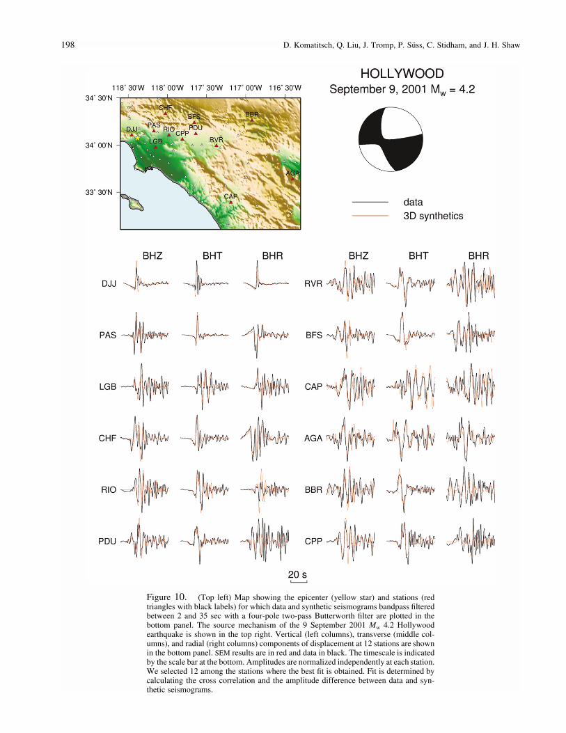
Figure 10. (Top left) Map showing the epicenter (yellow star) and stations (redtriangles with black labels) for which data and synthetic seismograms bandpass filteredbetween 2 and 35 sec with a four-pole two-pass Butterworth filter are plotted in thebottom panel. The source mechanism of the 9 September 2001 Mw 4.2 Hollywoodearthquake is shown in the top right. Vertical (left columns), transverse (middle col-umns), and radial (right columns) components of displacement at 12 stations are shownin the bottom panel. SEM results are in red and data in black. The timescale is indicatedby the scale bar at the bottom. Amplitudes are normalized independently at each station.We selected 12 among the stations where the best fit is obtained. Fit is determined bycalculating the cross correlation and the amplitude difference between data and syn-thetic seismograms.


118˚ 30'W

118˚ 30'W

118˚ 00'W

118˚ 00'W

117˚ 30'W

117˚ 30'W

33˚ 30'N 33˚ 30'N

34˚ 00'N 34˚ 00'N

34˚ 30'N 34˚ 30'N

0.2 0.4 0.6 0.8 1.0

(a)

118˚ 30'W

118˚ 30'W

118˚ 00'W

118˚ 00'W

117˚ 30'W

117˚ 30'W

33˚ 30'N 33˚ 30'N

34˚ 00'N 34˚ 00'N

34˚ 30'N 34˚ 30'N

0.2 0.4 0.6 0.8 1.0

(b)

118˚ 30'W

118˚ 30'W

118˚ 00'W

118˚ 00'W

117˚ 30'W

117˚ 30'W

33˚ 30'N 33˚ 30'N

34˚ 00'N 34˚ 00'N

34˚ 30'N 34˚ 30'N

0.2 0.4 0.6 0.8 1.0

(c)

Figure 11. Peak ground displacement (a), velocity (b), and acceleration (c) for the Hollywoodearthquake. Shown is a close-up on the Los Angeles basin. A value of 1 on the color scale corre-sponds to maxima of 0.80 mm, 0.92 mm s�1 and 2.15 mm s�2 for the norm of displacement,velocity, and acceleration at the surface, respectively. One can notice that amplification occurs inthe basin, where most of the energy is trapped, while hard-rock sites such as Palos Verdes, or themountains surrounding the Los Angeles and San Fernando basins, show little acceleration. Signifi-cant amplification occurs in the San Fernando valley, north of the epicenter, in particular near itseastern edge. Note that the peak ground velocity and acceleration maps are similar in character,while the peak ground displacement map is smoother in nature.

200 D. Komatitsch, Q. Liu, J. Tromp, P. Suss, C. Stidham, J. H. Shaw

119˚ 00'W

119˚ 00'W

118˚ 30'W

118˚ 30'W

118˚ 00'W

118˚ 00'W

117˚ 30'W

117˚ 30'W

33˚ 30'N 33˚ 30'N

34˚ 00'N 34˚ 00'N

34˚ 30'N 34˚ 30'N

100 secs.

SRNPLS

MLS

BRE

STG

RIO

LLS

RUS

LGB

STS

MWC

PAS

CHF

TA2

LAF

FMP

BCC

HLL

RPV

PDR

DJJ

ADO

LKL

LFP

SPF

PDE

ALP

TOV

MOP

BTP

OSI

LGU

STC

SES

Figure 12. Transverse component data (black) and 3D SEM synthetic seismograms(red) for the 3 September 2002 Yorba Linda event are plotted on a map of the LosAngeles area. Stations are denoted by blue triangles and labeled by their station codes.The instrument response was deconvolved from the data to obtain ground displacement.Both the data and the synthetic seismograms were subsequently bandpass filtered be-tween 6 and 35 sec with a four-pole two-pass Butterworth filter. The mechanism andlocation of the event are indicated by the black-and-white beach ball. The timescale isindicated by the scale bar at the bottom.

of the 3D model, not by the accuracy or the cost of thecalculations. Our current basin model is largely based uponP-wave speed information. Ground motions in the basin areto a large extent determined by S-wave speeds, which weestimate based upon a simple scaling relationship. Therefore,the basin model could be improved by adding constraints onthe S-wave speed and density structure, for instance basedupon borehole data (Stidham et al., 2001), as well as moreprecise P-wave speed constraints in subregions of the model.In a related effort, we are planning to use surface-wave phasedelays, such as those shown in Figure 9, as the starting pointfor an inversion for an improved S-wave model.

Because we are trying to fit signals in both amplitudeand phase, it is crucial that instruments are properly cali-brated, in particular in terms of timing, and that their ori-entation is precisely known. Otherwise, the inversion of am-plitude anomalies could be compromised by uncertaintiesrelated to station parameters.

Conclusions and Perspectives

We have demonstrated that ground motion in the LosAngeles basin can be modeled accurately based upon a re-cently developed basin model and a very precise numericaltechnique. The basin model is constrained by hundreds ofpetroleum-industry well logs and more than 20,000 km ofseismic reflection profiles. The numerical simulations arebased upon the SEM, which accounts for 3D variations ofseismic-wave speeds and density, topography and bathym-etry, and attenuation. They demonstrate that it is feasible topredict ground motion at periods longer than 2 sec usingrealistically complex models, thus improving our ability toassess seismic hazard. Peak ground displacement, velocity,and acceleration maps clearly illustrate that large amplifi-cation occurs within the basin.

Making use of the basin model in combination with theSEM allows one to invert for earthquake source parameters


119˚ 00'W

119˚ 00'W

118˚ 30'W

118˚ 30'W

118˚ 00'W

118˚ 00'W

117˚ 30'W

117˚ 30'W

33˚ 30'N 33˚ 30'N

34˚ 00'N 34˚ 00'N

34˚ 30'N 34˚ 30'N

100 secs.

SRN

WLT MLS

BRE

STG

RIO

LLS

LGBRVR

STS

MWC

PAS

CHF

TA2

LAF

FMP

BCC

HLL

RPV

PDR

DJJ

ADO

LKL

LFP

SPF

WSS

PDE

ALP

TOV

MOP

BTP

OSI

LGU

STC

SES

Figure 13. Transverse component data (black) and 1D SEM synthetic seismograms(green) for the 3 September 2002 Yorba Linda event are plotted on a map of the LosAngeles area. The background regional 1D model is that of Dreger and Helmberger(1990). Stations are denoted by blue triangles and labeled by their station codes. Theinstrument response was deconvolved from the data to obtain ground displacement.Both the data and the synthetic seismograms were subsequently bandpass filtered be-tween 6 and 35 sec with a four-pole two-pass Butterworth filter. The mechanism andlocation of the event are indicated by the black-and-white beach ball. The timescale isindicated by the scale bar at the bottom. Attenuation was not included in this 1Dcalculation.

by numerically calculating the necessary Frechet derivatives(Liu et al., 2002) and obtaining the estimated source param-eters by minimizing the waveform misfit between the dataand synthetic seismograms. Since a CMT inversion involvesof order 10 model parameters, the required simulations canbe done easily from a computational perspective. Our intentis to start performing CMT inversions routinely for all well-recorded future and past events above a certain magnitudethreshold. The resulting catalog of regional 3D CMT solu-tions should be very useful to the community and wouldcomplement existing catalogs based upon first-motion stud-ies and long-period surface waves.

An important future goal is to assess seismic risk forhypothetical large events by performing parametric studiesfor a number of earthquake scenarios. In this article, we haveused two small events to validate the basin model and the

numerical technique, while avoiding difficulties related tofinite-size sources and rupture velocity models for largerevents. However, the SEM is not limited to point sources: afinite-size source can be used by summing individual con-tributions from points located along the fault plane. Thisapproach can be used to calculate synthetic peak ground dis-placement, velocity, and acceleration maps, such as those inFigures 11 and 14, to assess seismic hazards associated withsuch large events.

Acknowledgments

The authors would like to thank Egill Hauksson and Jascha Polet forfirst-motion and surface-wave centroid moment tensor estimates, HirooKanamori for fruitful discussion, Steven M. Day for the analytical solutionof the SCEC LOH.3 benchmark, and TriNet for access to the data. They


118˚ 30'W

118˚ 30'W

118˚ 00'W

118˚ 00'W

117˚ 30'W

117˚ 30'W

33˚ 30'N 33˚ 30'N

34˚ 00'N 34˚ 00'N

34˚ 30'N 34˚ 30'N

0.2 0.4 0.6 0.8 1.0

(a)

118˚ 30'W

118˚ 30'W

118˚ 00'W

118˚ 00'W

117˚ 30'W

117˚ 30'W

33˚ 30'N 33˚ 30'N

34˚ 00'N 34˚ 00'N

34˚ 30'N 34˚ 30'N

0.2 0.4 0.6 0.8 1.0

(b)

118˚ 30'W

118˚ 30'W

118˚ 00'W

118˚ 00'W

117˚ 30'W

117˚ 30'W

33˚ 30'N 33˚ 30'N

34˚ 00'N 34˚ 00'N

34˚ 30'N 34˚ 30'N

0.2 0.4 0.6 0.8 1.0

(c)

Figure 14. Peak ground displacement (a), velocity (b), and acceleration (c) for the Yorba Lindaearthquake. A value of 1 corresponds to maxima of 0.64 mm, 0.94 mm s�1 and 2.02 mm s�2 forthe norm of displacement, velocity, and acceleration at the surface, respectively. Note that, as forthe Hollywood event in Figure 11, the peak ground velocity and acceleration maps are similar incharacter, but that the peak ground displacement map is smoother in nature. Again, hard-rock sitessuch as Palos Verdes and the mountains exhibit less amplification.


TopographyNo Topography

0 20 40 60 80Time (s)

Ver

tical

dis

plac

emen

t (�

m)

5

0

-5

(a)

AttenuationNo attenuation

20

10

0

-10

-200 50 100 150 200

Time (s)

Tran

sver

se d

ispl

acem

ent (

m)

�

(b)

Figure 15. (a) Vertical component displacement SEM synthetic seismogram for theYorba Linda earthquake recorded at MWC (Mount Wilson) when topography is in-cluded in the 3D simulations (solid line) and when a flat free surface is used (dashedline). (b) Transverse component for the Hollywood earthquake at station CAP (CapraRanch) with (solid line) and without (dashed line) attenuation. The results are filteredbetween 6 and 35 sec with a four-pole two-pass Butterworth filter. These seismogramsclearly show that the effect of topography and attenuation on seismic-wave propagationin the basin is not negligible.

also thank Thomas Pratt and an anonymous reviewer for comments thatimproved the manuscript. This research was funded in part by the NationalScience Foundation and by the National Earthquake Hazard Reduction Pro-gram under Grant 99HQGR001. This is Contribution Number 8966 of theDivision of Geological and Planetary Sciences, California Institute of Tech-nology.

References

Aagaard, B. T., J. F. Hall, and T. H. Heaton (2001). Characterization ofnear-source ground motions with earthquake simulations, EarthquakeSpectra 17, no. 2, 177–207.

Alex, C. M., and K. B. Olsen (1998). Lens effect in Santa Monica? Geo-phys. Res. Lett. 25, 3441–3444.

Anderson, J. G., Y. Lee, Y. Zeng, and S. M. Day (1996). Control of strongmotion by the upper 30 meters, Bull. Seism. Soc. Am. 86, 1749–1759.

Antolik, M., S. Larsen, D. Dreger, and B. Romanowicz (1996). Modelingbroadband waveforms in central California using finite differences,Seism. Res. Lett. 67, 30.

Apsel, R. J., and J. E. Luco (1983). On the Green’s functions for a layeredhalf-space, Bull. Seism. Soc. Am. 73, 931–951.

Bao, H., J. Bielak, O. Ghattas, L. F. Kallivokas, D. R. O’Hallaron, J. R.Shewchuk, and J. Xu (1998). Large-scale simulation of elastic wavepropagation in heterogeneous media on parallel computers, Comput.Methods Appl. Mech. Eng. 152, 85–102.

Berenger, J. P. (1994). A perfectly matched layer for the absorption ofelectromagnetic waves, J. Comput. Phys. 114, 185–200.

Bielak, J., J. Xu, and O. Ghattas (1999). Earthquake ground motion andstructural response in alluvial valleys, J. Geotech. Geoenv. Eng. 125,413–423.

Boore, D. M. (1972). Finite difference methods for seismic wave propa-gation in heterogeneous materials, in Methods in ComputationalPhysics, Vol. 11, Academic, New York.

Bouchon, M., and J. S. Barker (1996). Seismic response of a hill: the ex-ample of Tarzana, California, Bull. Seism. Soc. Am. 86, no. 1A,66–72.

Capdeville, Y., E. Chaljub, J. P. Vilotte, and J. P. Montagner (2003). Cou-pling the spectral element method with a modal solution for elasticwave propagation in global Earth models, Geophys. J. Int. 152,34–67.

Carcione, J. M., and P. J. Wang (1993). A Chebyshev collocation methodfor the wave equation in generalized coordinates, Comp. Fluid Dyn.J. 2, 269–290.

Catchings, R. D., and W. H. K. Lee (1996). Shallow velocity structure andPoisson’s ratio at the Tarzana, California, strong-motion accelerom-eter site, Bull. Seism. Soc. Am. 86, 1704–1713.

Chaljub, E. (2000). Modelisation numerique de la propagation d’ondes sis-miques en geometrie spherique: application a la sismologie globale(Numerical modeling of the propagation of seismic waves in sphericalgeometry: applications to global seismology), Ph.D. thesis, UniversiteParis VII Denis Diderot, Paris, France.

Chaljub, E., Y. Capdeville, and J. P. Vilotte (2003). Solving elastodynamicsin a fluid-solid heterogeneous sphere: a parallel spectral element ap-proximation on non-conforming grids, J. Comput. Phys. 187, no. 2,457–491.

Chew, W. C., and Q. Liu (1996). Perfectly matched layers for elastodyn-amics: a new absorbing boundary condition, J. Comput. Acoust. 4,no. 4, 341–359.

Clayton, R., and B. Engquist (1977). Absorbing boundary conditions foracoustic and elastic wave equations, Bull. Seism. Soc. Am. 67, 1529–1540.

Cohen, G., P. Joly, and N. Tordjman (1993). Construction and analysis ofhigher-order finite elements with mass lumping for the wave equation,in Proc. of the Second International Conference on Mathematical andNumerical Aspects of Wave Propagation, R. Kleinman (Editor),SIAM, Philadephia, Pennsylvania, 152–160.

Collino, F., and C. Tsogka (2001). Application of the PML absorbing layermodel to the linear elastodynamic problem in anisotropic heteroge-neous media, Geophysics 66, no. 1, 294–307.

Davis, P. M., J. L. Rubinstein, K. H. Liu, S. S. Gao, and L. Knopoff (2000).Northridge earthquake damage caused by geologic focusing of seis-mic waves, Science 289, 1746–1750.

Davis, T. L., J. Namson, and R. F. Yerkes (1989). A cross-section of the


120˚W

120˚W

118˚W

118˚W

116˚W

116˚W

34˚N 34˚N

36˚N 36˚N

100 secs.

SVD

DGR

ADO

CAPCIA

BBR

EDW

JVA

SCIEML

JCS

BOR

THX

BEL

TEH

OLP

HEC

LRL

GSC

SAL

CCC

SBC

BAK

ERR

ISA

DVT

CLCSLA

FIG

WES

DAN

VES

SMM

SPG

MTP

LDF

CWC

RCT

Figure 16. Transverse component data (black) and 3D SEM synthetic seismograms(red) for the 3 September 2002 Yorba Linda event are plotted on a map of southernCalifornia. Stations are denoted by blue triangles and labeled by their station codes.The instrument response was deconvolved from the data to obtain ground displacement.Both the data and the synthetic seismograms were subsequently bandpass filtered be-tween 6 and 35 sec with a four-pole two-pass Butterworth filter. In the Salton Sea area(for instance at stations SAL, ERR, and WES) and in the Mojave Desert (e.g., at stationADO), there is substantial low wave-speed sediment cover that is not yet included inour model, which causes resonance in the data that is not correctly reproduced.

Los Angeles area: seismically active fold-and-thrust belt, the 1987Whittier Narrows earthquake, and earthquake hazard, J. Geophys.Res. 94, 9644–9664.

Dreger, D. S., and D. V. Helmberger (1990). Broadband modeling of localearthquakes, Bull. Seism. Soc. Am. 80, 1162–1179.

Eisner, L., and R. W. Clayton (2002). A full waveform test of the southernCalifornia velocity model by the reciprocity method, Pure Appl. Geo-phys. 159, 1691–1706.

Faccioli, E., F. Maggio, R. Paolucci, and A. Quarteroni (1997). 2D and 3Delastic wave propagation by a pseudo-spectral domain decompositionmethod, J. Seism. 1, 237–251.

Frankel, A. (1993). Three-dimensional simulations of ground motions inthe San Bernardino valley, California, for hypothetical earthquakeson the San Andreas fault, Bull. Seism. Soc. Am. 83, 1020–1041.

Frankel, A., and W. Leith (1992). Evaluation of topographic effects on Pand S waves of explosions at the northern Novaya Zemlya test siteusing 3-D numerical simulations, Geophys. Res. Lett. 19, 1887–1890.

Frankel, A., and J. Vidale (1992). A three-dimensional simulation of seis-mic waves in the Santa Clara valley, California, from the Loma Prietaaftershock, Bull. Seism. Soc. Am. 82, 2045–2074.

Fuis, G. S., R. W. Clayton, P. M. Davis, T. Ryberg, W. J. Lutter, D. A.Okaya, E. Hauksson, C. Prodehl, J. M. Murphy, M. L. Benthien, S. A.Baher, M. D. Kohler, K. Thygesen, G. Simila, and G. R. Keller(2003). Fault systems of the 1971 San Fernando and 1994 Northridgeearthquakes, southern California: relocated aftershocks and seismicimages from LARSE II, Geology 31, 171–174.

Gaffet, S., and M. Bouchon (1989). Effects of two-dimensional topogra-phies using the discrete wavenumber-boundary integral equationmethod in P-SV cases, J. Acoust. Soc. Am. 85, 2277–2283.

Gao, S., H. Liu, P. M. Davis, and L. Knopoff (1996). Localized amplifi-cation of seismic waves and correlation with damage due to the North-ridge earthquake: evidence for focusing in Santa Monica, Bull. Seism.Soc. Am. 86, no. 18, S209–S230.


Garatani, K., H. Nakamura, H. Okuda, and G. Yagawa (2000). Large-scaleparallel wave propagation analysis by GeoFEM, Lect. Notes Comp.Sci. 1823, 445–453.

Graves, R. W. (1996). Simulating seismic wave propagation in 3D elasticmedia using staggered-grid finite differences, Bull. Seism. Soc. Am.86, no. 4, 1091–1106.

Graves, R. W. (1999). Three-dimensional computer simulations of realisticearthquake ground motions in regions of deep sedimentary basin, inThe Effects of Surface Geology on Seismic Motion, K. Irikura, K.Kudo, H. Okada, and T. Sasatani (Editors), Vol. 1, Balkema, Rotter-dam, The Netherlands, 103–120.

Gropp, W., E. Lusk, N. Doss, and A. Skjellum (1996). A high-performance,portable implementation of the MPI message passing interface stan-dard, Parallel Comput. 22, no. 6, 789–828.

Hadley, D., and H. Kanamori (1977). Seismic structure of the TransverseRanges, California, Geol. Soc. Am. Bull. 88, 1469–1478.

Hartzell, S., S. Harmsen, A. Frankel, D. Carver, E. Cranswick, M. Mere-monte, and J. Michael (1998). First-generation site-response maps forthe Los Angeles region based on earthquake ground motions, Bull.Seism. Soc. Am. 88, 463–472.

Hartzell, S. H., A. Leeds, A. Frankel, and J. Michael (1996). Site responsefor urban Los Angeles using aftershocks of the Northridge earth-quake, Bull. Seism. Soc. Am. 86, no. 18, S168–S192.

Hauksson, E. (1990). Earthquakes, faulting, and stress in the Los Angelesbasin, J. Geophys. Res. 95, 15,365–15,394.

Hauksson, E. (2000). Crustal structure and seismicity distribution adjacentto the Pacific and North America plate boundary in southern Califor-nia, J. Geophys. Res. 105, 13,875–13,903.

Hauksson, E., and J. S. Haase (1997). Three-dimensional Vp and Vp/Vs

velocity models of the Los Angeles basin and central TransverseRanges, California, J. Geophys. Res. 102, 5423–5453.

Hauksson, E., T. L. Teng, and T. L. Henyey (1987). Results from a 1500 mdeep, three-level downhole seismometer array: site response, low Qvalues, and f max, Bull. Seism. Soc. Am. 77, 1883–1904.

Huftile, G. J., and R. S. Yeats (1995). Convergence rates across a displace-ment transfer zone in the western Transverse Ranges, Ventura basin,California, J. Geophys. Res. 100, no. 2, 2043–2067.

Ichinose, G. A., S. M. Day, H. Magistrale, T. Prush, F. Vernon, and A.Edelman (1996). Crustal thickness variations beneath the PeninsularRanges, southern California, Geophys. Res. Lett. 23, 3095–3098.

Igel, H. (1999). Wave propagation in three-dimensional spherical sectionsby the Chebyshev spectral method, Geophys. J. Int. 136, 559–566.

Jennings, P. (1975). Fault map of California with volcanoes, thermalsprings, and thermal wells at 1:750,000 scale, in Geological Data Map1, California Division of Mines and Geology, Sacramento, California.

Ji, C., D. V. Helmberger, and D. J. Wald (2000). Basin structure estimationby waveform modeling: forward and inverse methods, Bull. Seism.Soc. Am. 90, 964–976.

Ji, C., D. J. Wald, and D. V. Helmberger (2002). Source description of the1999 Hector Mine, California earthquake, part I: Wavelet domaininversion theory and resolution analysis, Bull. Seism. Soc. Am. 92,1192–1207.

Komatitsch, D. (1997). Methodes spectrales et elements spectraux pourl’equation de l’elastodynamique 2D et 3D en milieu heterogene(Spectral and spectral-element methods for the 2D and 3D elastodyn-amics equations in heterogeneous media), Ph.D. thesis, Institut dePhysique du Globe, Paris, France.

Komatitsch, D., and J. Tromp (1999). Introduction to the spectral-elementmethod for 3-D seismic wave propagation, Geophys. J. Int. 139, 806–822.

Komatitsch, D., and J. Tromp (2001). Modeling of seismic wave propa-gation at the scale of the Earth on a large Beowulf, Proc. of the ACM/IEEE Supercomputing SC’2001 Conference, Denver, Colorado, 10–16 November 2001, CD-ROM, www.sc-conference.org/.

Komatitsch, D., and J. Tromp (2002a). Spectral-element simulations ofglobal seismic wave propagation, I. Validation, Geophys. J. Int. 149,390–412.

Komatitsch, D., and J. Tromp (2002b). Spectral-element simulations ofglobal seismic wave propagation, II. 3-D models, oceans, rotation,and self-gravitation, Geophys. J. Int. 150, 303–318.

Komatitsch, D., and J. Tromp (2003). A perfectly matched layer absorbingboundary condition for the second-order seismic wave equation, Geo-phys. J. Int. 154, 146–153.

Komatitsch, D., and J. P. Vilotte (1998). The spectral-element method: anefficient tool to simulate the seismic response of 2D and 3D geologicalstructures, Bull. Seism. Soc. Am. 88, no. 2, 368–392.

Komatitsch, D., S. Tsuboi, C. Ji, and J. Tromp (2003). A 14.6 billion de-grees of freedom, 5 teraflops, 2.5 terabyte earthquake simulation onthe Earth Simulator, Proc. of the ACM/IEEE SupercomputingSC’2003 Conference, Phoenix, Arizona, 15–21 November, CD-ROM,www.sc-conference.org.

Komatitsch, D., J. P. Vilotte, R. Vai, J. M. Castillo-Covarrubias, and F. J.Sanchez-Sesma (1999). The spectral element method for elastic waveequations: application to 2D and 3D seismic problems, Int. J. Numer.Meth. Eng. 45, 1139–1164.

Kristek, J., P. Moczo, K. Irikura, T. Iwata, and H. Sekiguchi (1999). The1995 Kobe mainshock simulated by 3D finite differences, in The Ef-fects of Surface Geology on Seismic Motion, K. Irikura, K. Kudo,H. Okada, and T. Sasatani (Editors), Vol. 3, Balkema, Rotterdam, TheNetherlands, 1361–1368.

Larsen, S., M. Antolik, D. Dreger, C. Stidham, C. Schultz, A. Lomax, andB. Romanowicz (1997). 3-D models of seismic wave propagation:Simulating scenario earthquakes along the Hayward fault, Seism. Res.Lett. 68, 328.

Lewis, J., S. M. Day, H. Magistrale, J. Eakins, and F. L. Vernon (2000).Crustal thickness of the Peninsular Ranges, southern California, fromteleseismic receiver functions, Geology 28, 303–306.

Liu, Q., D. Komatitsch, and J. Tromp (2002). Spectral-element centroid-moment tensor inversions, EOS 83.

Luyendyk, B. P., and J. S. Hornafius (1987). Neogene crustal rotations,fault slip and basin development in southern California, in CenozoicBasin Development of Coastal California, R. V. Ingersoll and W. G.Ernst (Editors), Prentice Hall, New York, 259–283.

Lysmer, J., and L. A. Drake (1972). A finite element method for seismol-ogy, in Methods in Computational Physics, Vol. 11, Academic, NewYork.

Magistrale, H., S. Day, R. W. Clayton, and R. Graves (2000). The SCECSouthern California reference three-dimensional seismic velocitymodel version 2, Bull. Seism. Soc. Am. 90, S65–S76.

Magistrale, H., K. McLaughlin, and S. Day (1996). A geology based 3-Dvelocity model of the Los Angeles basin sediments, Bull. Seism. Soc.Am. 86, 1161–1166.

McCulloh, T. H. (1960). Gravity variations and the geology of the LosAngeles basin of California, U.S. Geol. Surv. Profess. Pap. 400-B,320–325.

McLaughlin, K. L., and S. M. Day (1994). 3-D elastic finite-differenceseismic wave simulations, Comput. Phys. 8, no. 6, 656–663.

Moczo, P., E. Bystricky, J. Kristek, J. M. Carcione, and M. Bouchon (1997).Hybrid modeling of P-SV seismic motion at inhomogeneous visco-elastic topographic structures, Bull. Seism. Soc. Am. 87, 1305–1323.

Namson, J., and T. L. Davis (1992). Late Cenozoic thrust ramps of southernCalifornia, technical report, Davis & Namson Consulting Geologists,Valencia, California, unpublished report.

Olsen, K. B. (2000). Site amplification in the Los Angeles basin from three-dimensional modeling of ground motion, Bull. Seism. Soc. Am. 90,S77–S94.

Olsen, K. B., and R. J. Archuleta (1996). 3-D simulation of earthquakes onthe Los Angeles fault system, Bull. Seism. Soc. Am. 86, no. 3, 575–596.

Olsen, K. B., S. M. Day, and C. R. Bradley (2003). Estimation of Q forlong-period (�2 sec) waves in the Los Angeles basin, Bull. Seism.Soc. Am. 93, no. 2, 627–638.

Olsen, K. B., R. Madariaga, and R. J. Archuleta (1997). Three-dimensional


dynamic simulation of the 1992 Landers earthquake, Science 278,834–838.

Olsen, K. B., J. C. Pechmann, and G. T. Schuster (1995). Simulation of 3-D elastic wave propagation in the Salt Lake basin, Bull. Seism. Soc.Am. 85, 1688–1710.

Patera, A. T. (1984). A spectral element method for fluid dynamics: laminarflow in a channel expansion, J. Comput. Phys. 54, 468–488.

Peyrat, S., K. B. Olsen, and R. Madariaga (2001). Dynamic modeling ofthe 1992 Landers earthquake, J. Geophys. Res. 106, 26,467–26,482.

Pitarka, A., and K. Irikura (1996a). Modeling 3D surface topography by afinite-difference method: Kobe–JMA station site, Japan, case study,Geophys. Res. Lett. 23, 2729–2732.

Pitarka, A., and K. Irikura (1996b). Basin structure effects on long periodstrong motions in the San Fernando valley and the Los Angeles basinfrom the 1994 Northridge earthquake and aftershocks, Bull. Seism.Soc. Am. 86, no. 18, S126–S137.

Priolo, E., J. M. Carcione, and G. Seriani (1994). Numerical simulation ofinterface waves by high-order spectral modeling techniques, J.Acoust. Soc. Am. 95, no. 2, 681–693.

Rial, J. A. (1996). The anomalous seismic response of the ground at theTarzana Hill site during the Northridge 1994 Southern Californiaearthquake: a resonant, sliding block? Bull. Seism. Soc. Am. 86, 1714–1723.

Satoh, T., H. Kawase, T. Sato, and A. Pitarka (2001). Three-dimensionalfinite-difference waveform modeling of strong motions observed inthe Sendai basin, Japan, Bull. Seism. Soc. Am. 91, 365–380.

Schneider, C. L., C. Hummon, R. S. Yeats, and G. J. Huftile (1996). Struc-tural evolution of the northern Los Angeles basin, California, basedon growth strata, Tectonics 15, 341–355.

Seriani, G., and E. Priolo (1994). A spectral element method for acousticwave simulation in heterogeneous media, Finite Elem. Anal. Des. 16,337–348.

Shaw, J. H., and P. Shearer (1999). An elusive blind-thrust fault beneathmetropolitan Los Angeles, Science 283, 1516–1518.

Shaw, J. H., and J. Suppe (1996). Earthquake hazards of active blind-thrustfaults under the central Los Angeles basin, California, J. Geophys.Res. 101, 8623–8642.

Spudich, P., M. Hellweg, and W. H. K. Lee (1996). Directional topographicsite response at Tarzana observed in aftershocks of the 1994 North-ridge, California, earthquake: implications for mainshock motions,Bull. Seism. Soc. Am. 86, no. 18, S193–S208.

Stevens, J. L., K. L. McLaughlin, B. Shkoller, and S. M. Day (1993). 2-Daxisymmetric calculations of surface waves generated by an explosionin an island, mountain and sedimentary basin, Geophys. J. Int. 114,548–560.

Stidham, C., M. Antolik, D. Dreger, S. Larsen, and B. Romanowicz (1999).Three-dimensional structure influences on the strong motion wave-field of the 1989 Loma Prieta earthquake, Bull. Seism. Soc. Am. 89,1184–1202.

Stidham, C., M. P. Suss, and J. H. Shaw (2001). 3D density and velocitymodel of the Los Angeles basin, in Geological Society of America2001 Annual Meeting Abstracts, Denver, Colorado, Geological So-ciety of America, 33, 299.

Suss, M. P., and J. H. Shaw (2003). P-wave seismic velocity structurederived from sonic logs and industry reflection data in the Los An-geles basin, California, J. Geophys. Res. 108 B3 ESE13, 1–18.

Tessmer, E., D. Kessler, D. Kosloff, and A. Behle (1992). Multi-domainChebyshev-Fourier method for the solution of the equations of motionof dynamic elasticity, J. Comput. Phys. 100, 355–363.

U.S. Geological Survey (2003) (USGS). U. S. Geological Survey SouthernCalifornia topography map, www.usgs.gov (last accessed December2003).

Virieux, J. (1986). P-SV wave propagation in heterogeneous media: velocity-stress finite-difference method, Geophysics 51, 889–901.

Wald, D. J., and R. W. Graves (1998). The seismic response of the LosAngeles basin, California, Bull. Seism. Soc. Am. 88, 337–356.

Wald, D. J., T. H. Heaton, and K. W. Hudnut (1996). The slip history ofthe 1994 Northridge, California, earthquake determined from strongground motion, teleseismic, GPS, and leveling data, Bull. Seism. Soc.Am. 86, S49–S70.

Wright, T. L. (1991). Structural geology and tectonic evolution of the LosAngeles basin, California, in Active Margin Basins, K. T. Biddle (Ed-itor), Am. Assoc. Pet. Geol. Memoir, Vol. 52, 35–134.

Yeats, R. S., G. J. Huftile, and L. T. Stitt (1994). Late Cenozoic tectonicsof the east Ventura basin, Transverse Ranges, California, Am. Assoc.Petrol. Geol. Bull. 78, no. 7, 1040–1074.

Zahradnık, J., P. Moczo, and F. Hron (1993). Testing four elastic finite-difference schemes for behavior at discontinuities, Bull. Seism. Soc.Am. 83, 107–129.

Zhu, L., and H. Kanamori (2000). Moho depth variation in southern Cali-fornia from teleseismic receiver functions, J. Geophys. Res. 105,2969–2980.

Seismological LaboratoryCalifornia Institute of Technology1200 E. California Blvd.Pasadena, California 91125

(D.K., Q.L., J.T.)

Department of Earth and Planetary SciencesHarvard University20 Oxford St.Cambridge, Massachusetts 02138

(P.S., C.S., J.H.S.)

Manuscript received 21 April 2003.

Date post:	19-Mar-2018
Category:	Documents
Upload:	trinhthu
View:	215 times
Download:	1 times

Simulations of Ground Motion in the Los Angeles Basin...

Documents