Simultaneous Flow of Immiscible Fluids • Purpose: predict the displacement of oil by water • Organization: – development of equations of multiphase, immiscible flow • concluding with the frontal advance and Buckley-Leverett equations. – factors that control displacement efficiency – limitations of immiscible displacement solutions
Transcript
Simultaneous Flow of Immiscible Fluids
• Purpose: predict the displacement of oil by water
• Organization: – development of equations of multiphase, immiscible flow
• concluding with the frontal advance and Buckley-Leverett equations.
– factors that control displacement efficiency
– limitations of immiscible displacement solutions
Simultaneous Flow of Immiscible Fluids
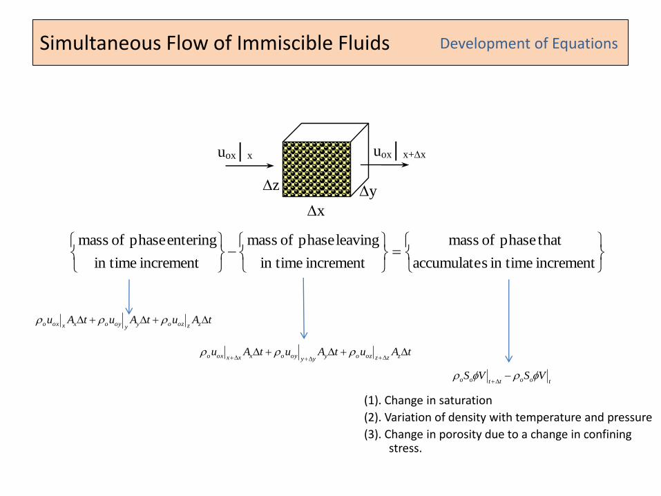
(1). Change in saturation
(2). Variation of density with temperature and pressure
(3). Change in porosity due to a change in confining stress.
increment in time saccumulate
thatphase of mass
increment in time
leaving phase of mass
increment in time
entering phase of mass
uox│x uox│x+x
x
y z
Development of Equations
tAutAutAu zzozoyyoyoxxoxo
tAutAutAu zzzozoyyyoyoxxxoxo
toottoo VSVS
Simultaneous Flow of Immiscible Fluids
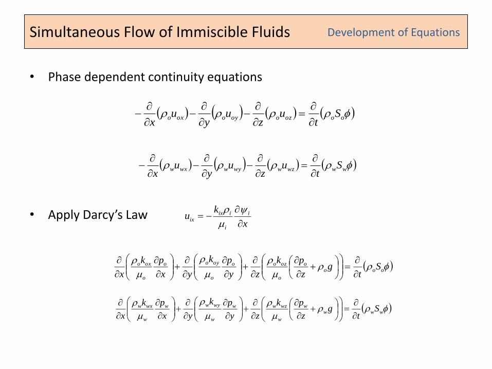
• Phase dependent continuity equations
• Apply Darcy’s Law
Development of Equations
ooozooyooxo St
uz
uy
ux
wwwzwwywwxw St
uz
uy
ux
x
ku i
i
iixix
ooo
o
o
ozoo
o
oyoo
o
oxo St
gz
pk
zy
pk
yx
pk
x
www
w
w
wzww
w
wyww
w
wxw St
gz
pk
zy
pk
yx
pk
x
Simultaneous Flow of Immiscible Fluids
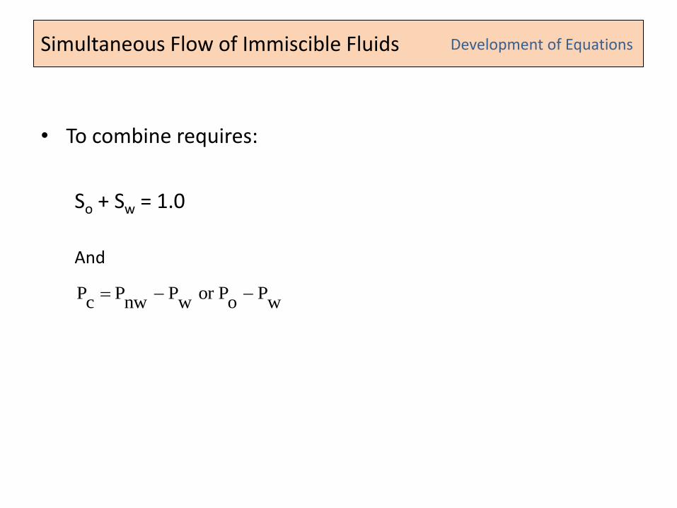
• To combine requires:
So + Sw = 1.0
And
Development of Equations
wP
oPor
wP
nwP
cP
Simultaneous Flow of Immiscible Fluids
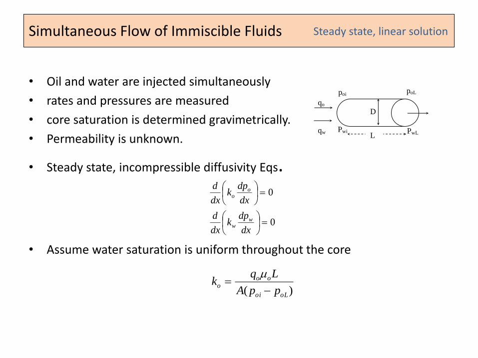
• Oil and water are injected simultaneously
• rates and pressures are measured
• core saturation is determined gravimetrically.
• Permeability is unknown.
• Steady state, incompressible diffusivity Eqs.
• Assume water saturation is uniform throughout the core
Steady state, linear solution
qo
qw L
poi
Pwi
poL
PwL
D
0
0
dx
dpk
dx
d
dx
dpk
dx
d
ww
oo
)( oLoi
ooo
ppA
Lqk
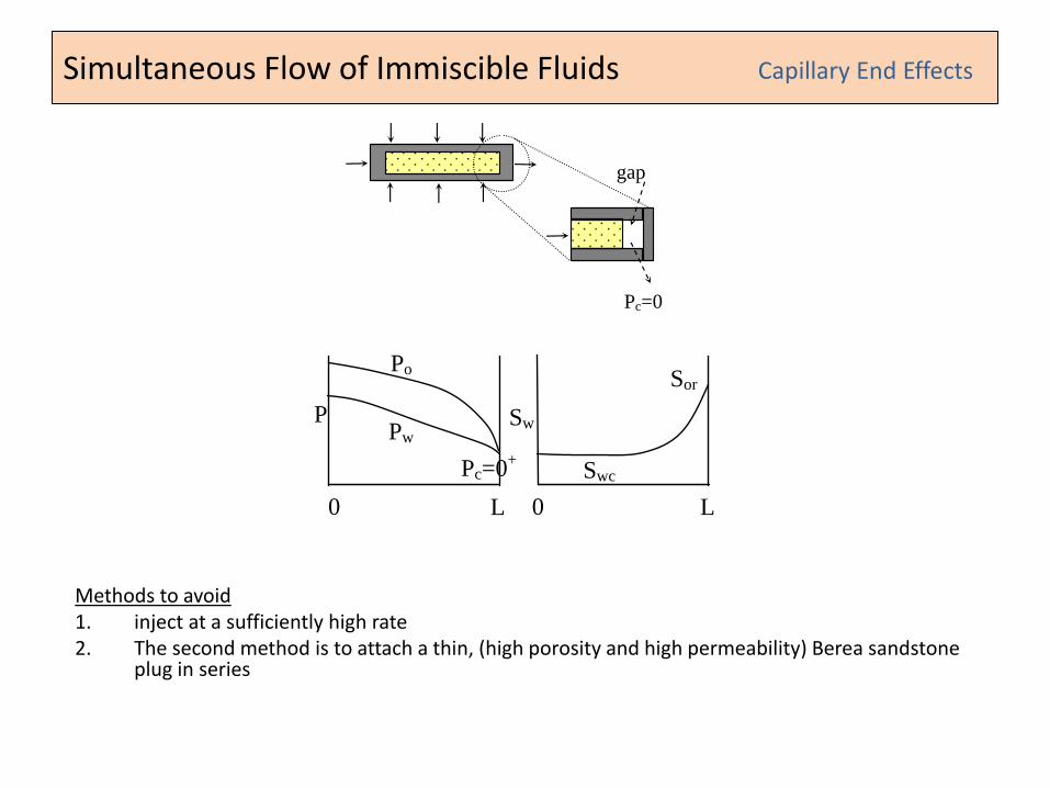
Simultaneous Flow of Immiscible Fluids
Methods to avoid 1. inject at a sufficiently high rate 2. The second method is to attach a thin, (high porosity and high permeability) Berea sandstone
plug in series
Capillary End Effects
gap
Pc=0
Sw
0 0 L L
Po
Pw
Pc=0+ Swc
Sor
P
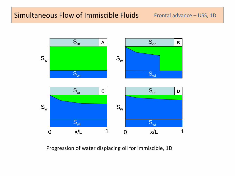
Simultaneous Flow of Immiscible Fluids Frontal advance – USS, 1D
Swi
Sor
Sw
A
Swi
Sor
Sw
C
0 1x/L
Swi
Sor
Sw
B
Swi
Sor
Sw
D
0 1x/L
Swi
Sor
Sw
A
Swi
Sor
Sw
A
Swi
Sor
Sw
C
0 1x/L
Swi
Sor
Sw
B
Swi
Sor
Sw
B
Swi
Sor
Sw
D
0 1x/L
Progression of water displacing oil for immiscible, 1D
Simultaneous Flow of Immiscible Fluids
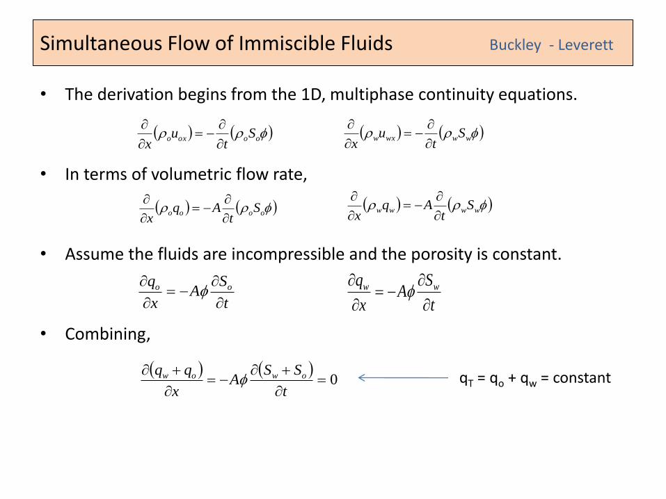
• The derivation begins from the 1D, multiphase continuity equations.
• In terms of volumetric flow rate,
• Assume the fluids are incompressible and the porosity is constant.
• Combining,
Buckley - Leverett
oooxo St
ux
wwwxw S
tu
x
t
SA
x
q oo
t
SA
x
q ww
oooo St
Aqx
wwww St
Aqx
0
t
SSA
x
qq owow qT = qo + qw = constant
Simultaneous Flow of Immiscible Fluids
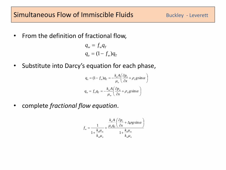
• From the definition of fractional flow,
• Substitute into Darcy’s equation for each phase,
• complete fractional flow equation.
Buckley - Leverett
Two
Tww
qfq
qfq
)1(
sin)1( gx
pAkqfq o
o
o
oTwo
singx
pAkqfq w
w
w
wTww
ow
wo
c
To
o
ow
wow
k
k
gx
p
q
Ak
k
kf
1
sin
1
1
Simultaneous Flow of Immiscible Fluids
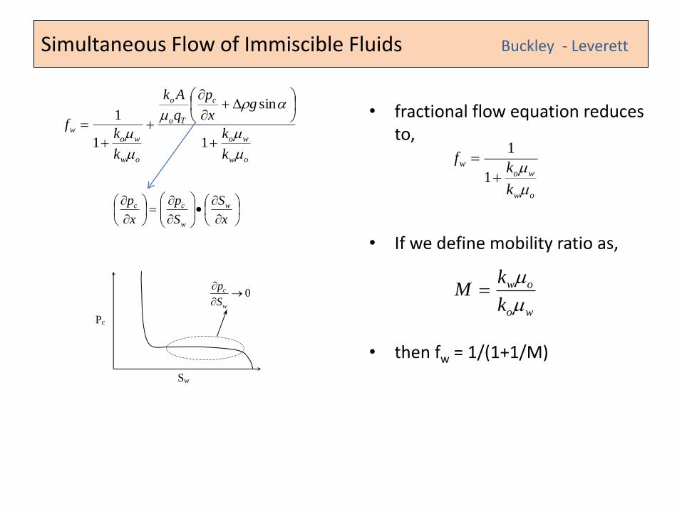
• fractional flow equation reduces to,
• If we define mobility ratio as,
• then fw = 1/(1+1/M)
Buckley - Leverett
ow
wo
c
To
o
ow
wow
k
k
gx
p
q
Ak
k
kf
1
sin
1
1
x
S
S
p
x
p w
w
cc
Sw
Pc
0
w
c
S
p
ow
wow
k
kf
1
1
wo
ow
k
kM
Simultaneous Flow of Immiscible Fluids
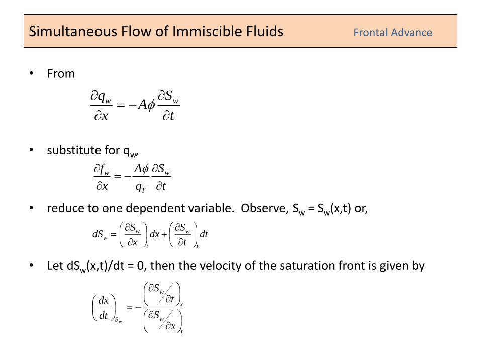
• From
• substitute for qw,
• reduce to one dependent variable. Observe, Sw = Sw(x,t) or,
• Let dSw(x,t)/dt = 0, then the velocity of the saturation front is given by
Frontal Advance
t
SA
x
q ww
t
S
q
A
x
f w
T
w
dtt
Sdx
x
SdS
t
w
t
ww
t
w
x
w
S
xS
tS
dt
dx
w
Simultaneous Flow of Immiscible Fluids
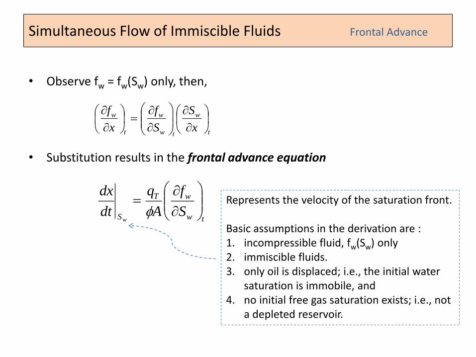
• Observe fw = fw(Sw) only, then,
• Substitution results in the frontal advance equation
Frontal Advance
t
w
tw
w
t
w
x
S
S
f
x
f
tw
wT
S S
f
A
q
dt
dx
w
Represents the velocity of the saturation front. Basic assumptions in the derivation are : 1. incompressible fluid, fw(Sw) only 2. immiscible fluids. 3. only oil is displaced; i.e., the initial water
saturation is immobile, and 4. no initial free gas saturation exists; i.e., not
a depleted reservoir.
Simultaneous Flow of Immiscible Fluids
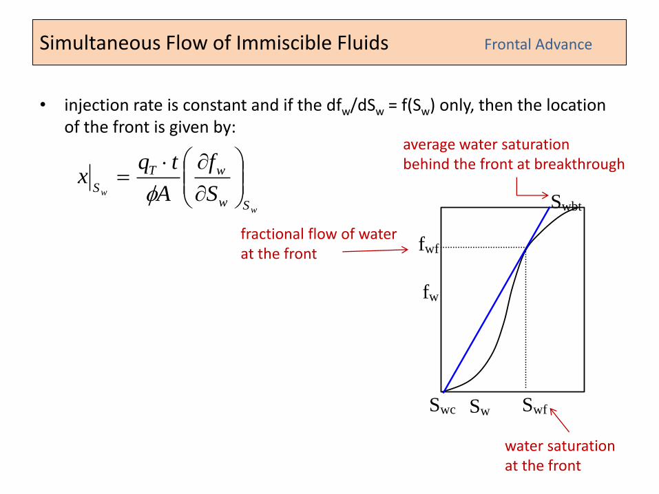
• injection rate is constant and if the dfw/dSw = f(Sw) only, then the location of the front is given by:
Frontal Advance
Swf Sw Swc
fw
fwf
Swbt w
w
Sw
wT
S S
f
A
tqx
fractional flow of water at the front
water saturation at the front
average water saturation behind the front at breakthrough
Simultaneous Flow of Immiscible Fluids
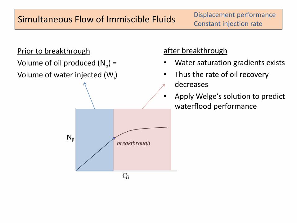
Prior to breakthrough
Volume of oil produced (Np) =
Volume of water injected (Wi)
Displacement performance Constant injection rate
Np
Qi
breakthrough
after breakthrough
• Water saturation gradients exists
• Thus the rate of oil recovery decreases
• Apply Welge’s solution to predict waterflood performance
Simultaneous Flow of Immiscible Fluids
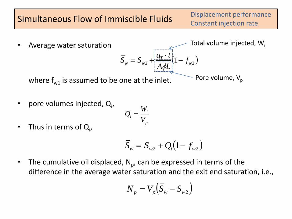
• Average water saturation
where fw1 is assumed to be one at the inlet.
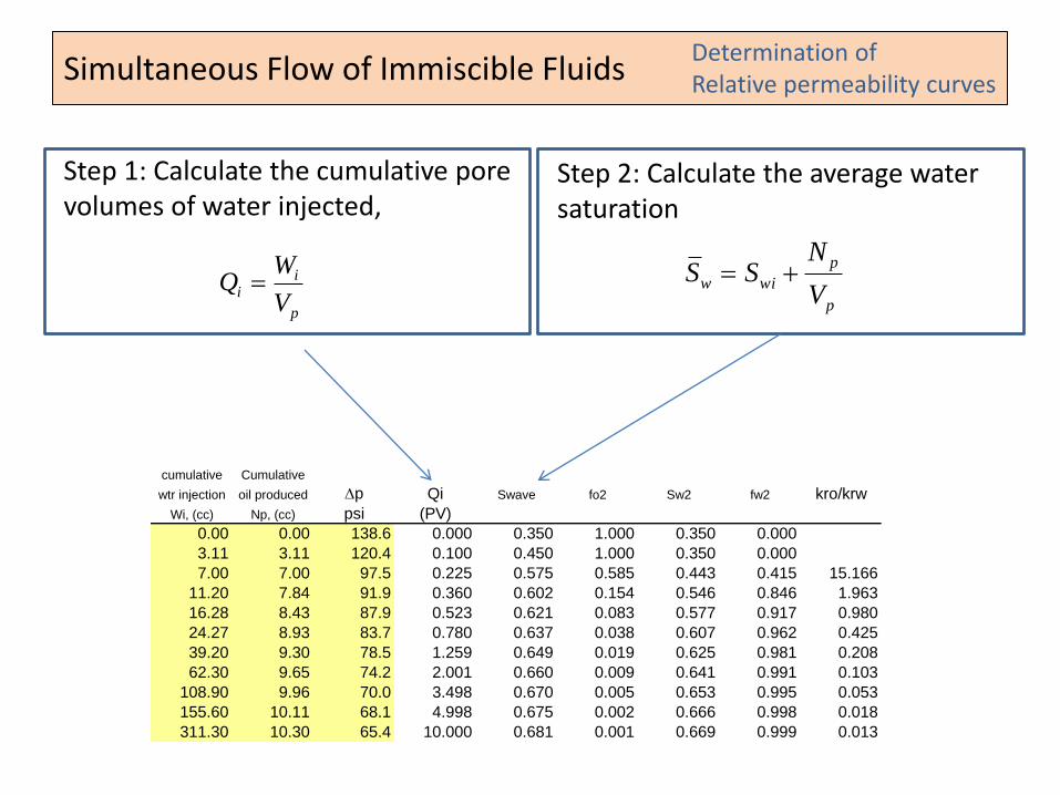
• pore volumes injected, Qi,
• Thus in terms of Qi,
• The cumulative oil displaced, Np, can be expressed in terms of the difference in the average water saturation and the exit end saturation, i.e.,
Displacement performance Constant injection rate
22 1 wT
ww fLA
tqSS
p
ii
V
WQ
22 1 wiww fQSS
2wwpp SSVN
Total volume injected, Wi
Pore volume, Vp
Simultaneous Flow of Immiscible Fluids
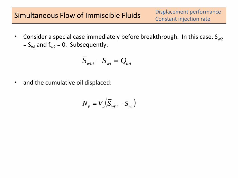
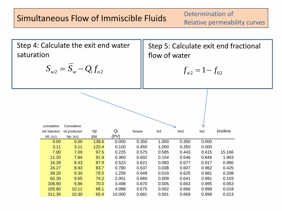
• Consider a special case immediately before breakthrough. In this case, Sw2 = Swi and fw2 = 0. Subsequently:
• and the cumulative oil displaced:
Displacement performance Constant injection rate
ibtwiwbt QSS
wiwbtpp SSVN
Simultaneous Flow of Immiscible Fluids
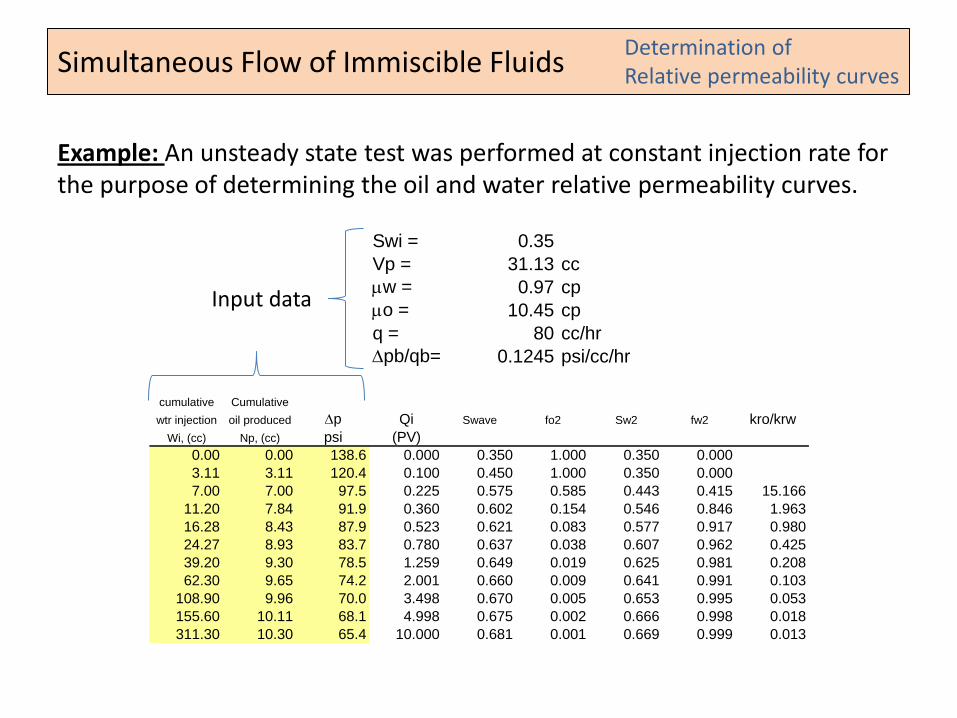
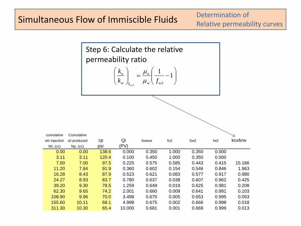
Example: An unsteady state test was performed at constant injection rate for the purpose of determining the oil and water relative permeability curves.
Determination of Relative permeability curves
Swi = 0.35
Vp = 31.13 cc
w = 0.97 cp
o = 10.45 cp
q = 80 cc/hr
pb/qb= 0.1245 psi/cc/hr
cumulative Cumulative
wtr injection oil produced p Qi Swave fo2 Sw2 fw2 kro/krw
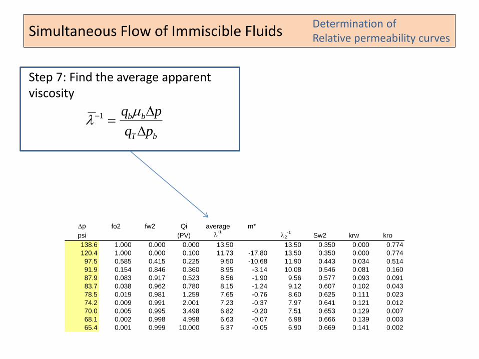
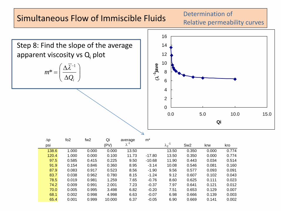
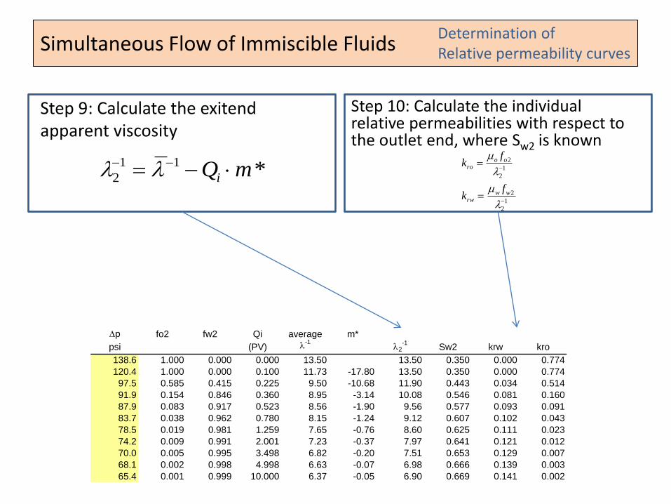
Step 10: Calculate the individual relative permeabilities with respect to the outlet end, where Sw2 is known
*11
2 mQi 1
2
2
1
2
2
wwrw
ooro
fk
fk
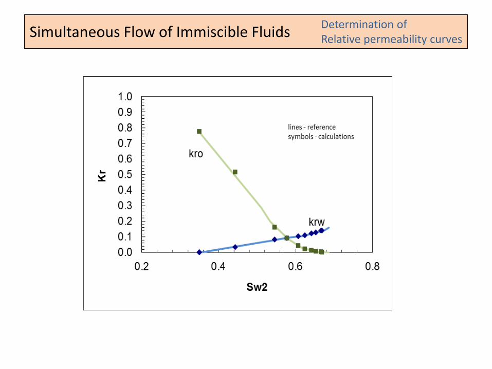
Simultaneous Flow of Immiscible Fluids Determination of Relative permeability curves
Simultaneous Flow of Immiscible Fluids
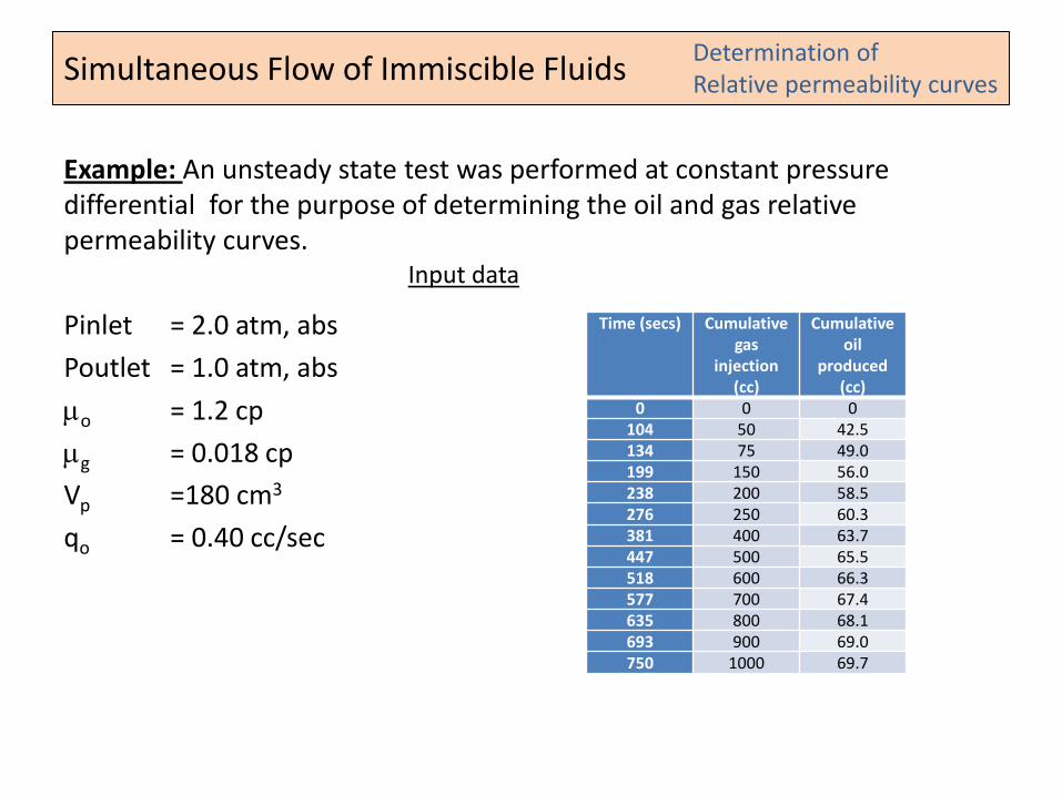
Example: An unsteady state test was performed at constant pressure differential for the purpose of determining the oil and gas relative permeability curves.
Pinlet = 2.0 atm, abs
Poutlet = 1.0 atm, abs
o = 1.2 cp
g = 0.018 cp
Vp =180 cm3
qo = 0.40 cc/sec
Determination of Relative permeability curves
Input data
Time (secs) Cumulative gas
injection (cc)
Cumulative oil
produced (cc)
0 0 0
104 50 42.5
134 75 49.0
199 150 56.0
238 200 58.5
276 250 60.3
381 400 63.7
447 500 65.5
518 600 66.3
577 700 67.4
635 800 68.1
693 900 69.0
750 1000 69.7
Simultaneous Flow of Immiscible Fluids
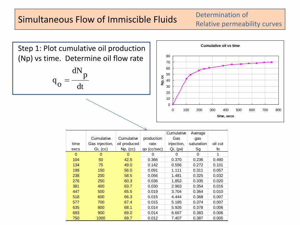
Step 1: Plot cumulative oil production (Np) vs time. Determine oil flow rate
Determination of Relative permeability curves
time
secs
Cumulative
Gas injection,
Gi, (cc)
Cumulative
oil produced
Np, (cc)
production
rate
qo (cc/sec)
Cumulative
Gas
injection,
Qi, (pv)
Average
gas
saturation
Sg
oil cut
fo
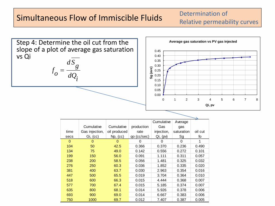
0 0 0 0 0 0 1
104 50 42.5 0.366 0.370 0.236 0.490
134 75 49.0 0.142 0.556 0.272 0.101
199 150 56.0 0.091 1.111 0.311 0.057
238 200 58.5 0.056 1.481 0.325 0.032
276 250 60.3 0.036 1.852 0.335 0.020
381 400 63.7 0.030 2.963 0.354 0.016
447 500 65.5 0.019 3.704 0.364 0.010
518 600 66.3 0.015 4.444 0.368 0.007
577 700 67.4 0.015 5.185 0.374 0.007
635 800 68.1 0.014 5.926 0.378 0.006
693 900 69.0 0.014 6.667 0.383 0.006
750 1000 69.7 0.012 7.407 0.387 0.005
dt
pdN
oq
Cumulative oil vs time
0
10
20
30
40
50
60
70
80
0 100 200 300 400 500 600 700 800
time, secs
Np
, cc
Simultaneous Flow of Immiscible Fluids
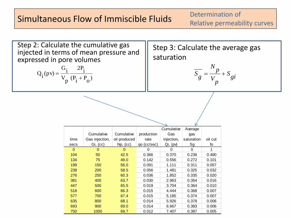
Step 2: Calculate the cumulative gas injected in terms of mean pressure and expressed in pore volumes
Determination of Relative permeability curves
Step 3: Calculate the average gas saturation
time
secs
Cumulative
Gas injection,
Gi, (cc)
Cumulative
oil produced
Np, (cc)
production
rate
qo (cc/sec)
Cumulative
Gas
injection,
Qi, (pv)
Average
gas
saturation
Sg
oil cut
fo
0 0 0 0 0 0 1
104 50 42.5 0.366 0.370 0.236 0.490
134 75 49.0 0.142 0.556 0.272 0.101
199 150 56.0 0.091 1.111 0.311 0.057
238 200 58.5 0.056 1.481 0.325 0.032
276 250 60.3 0.036 1.852 0.335 0.020
381 400 63.7 0.030 2.963 0.354 0.016
447 500 65.5 0.019 3.704 0.364 0.010
518 600 66.3 0.015 4.444 0.368 0.007
577 700 67.4 0.015 5.185 0.374 0.007
635 800 68.1 0.014 5.926 0.378 0.006
693 900 69.0 0.014 6.667 0.383 0.006
750 1000 69.7 0.012 7.407 0.387 0.005
)o
Pi
P(
iP2
pV
iG
)pv(i
Q
gi
S
pV
pN
gS
Simultaneous Flow of Immiscible Fluids
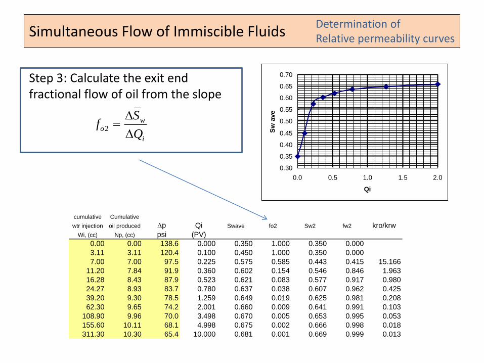
Step 4: Determine the oil cut from the slope of a plot of average gas saturation vs Qi
Determination of Relative permeability curves
time
secs
Cumulative
Gas injection,
Gi, (cc)
Cumulative
oil produced
Np, (cc)
production
rate
qo (cc/sec)
Cumulative
Gas
injection,
Qi, (pv)
Average
gas
saturation
Sg
oil cut
fo
0 0 0 0 0 0 1
104 50 42.5 0.366 0.370 0.236 0.490
134 75 49.0 0.142 0.556 0.272 0.101
199 150 56.0 0.091 1.111 0.311 0.057
238 200 58.5 0.056 1.481 0.325 0.032
276 250 60.3 0.036 1.852 0.335 0.020
381 400 63.7 0.030 2.963 0.354 0.016
447 500 65.5 0.019 3.704 0.364 0.010
518 600 66.3 0.015 4.444 0.368 0.007
577 700 67.4 0.015 5.185 0.374 0.007
635 800 68.1 0.014 5.926 0.378 0.006
693 900 69.0 0.014 6.667 0.383 0.006
750 1000 69.7 0.012 7.407 0.387 0.005
idQ
gSd
of
Average gas saturation vs PV gas injected
0.00
0.05
0.10
0.15
0.20
0.25
0.30
0.35
0.40
0.45
0 1 2 3 4 5 6 7 8
Qi, pv
Sg
(av
e)
Simultaneous Flow of Immiscible Fluids
Step 5: Determine the relative permeability ratio
Determination of Relative permeability curves
Step 6: Calculate the saturation at the outflow face
o
g
of
of1
rok
rgk
of
iQ
gS
gS *
2
Cumulative
Gas injection,
Qi, (pv)
Average gas
saturation
Sg krg/kro ratio
Exit end
saturation
Sg2
Exit end
saturation
So2 Kro Krg
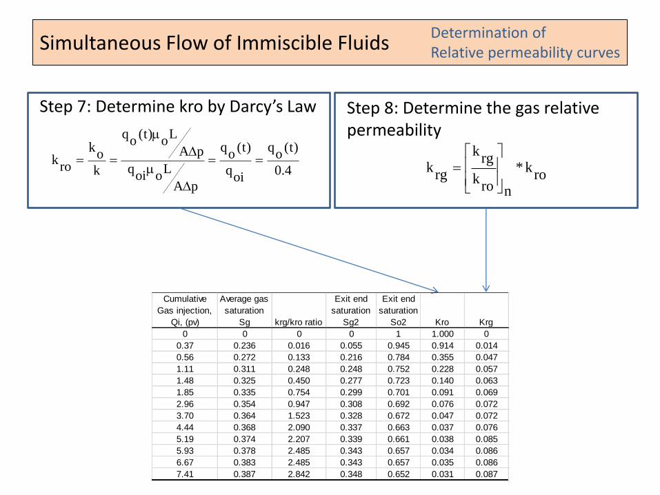
0 0 0 0 1 1.000 0
0.37 0.236 0.016 0.055 0.945 0.914 0.014
0.56 0.272 0.133 0.216 0.784 0.355 0.047
1.11 0.311 0.248 0.248 0.752 0.228 0.057
1.48 0.325 0.450 0.277 0.723 0.140 0.063
1.85 0.335 0.754 0.299 0.701 0.091 0.069
2.96 0.354 0.947 0.308 0.692 0.076 0.072
3.70 0.364 1.523 0.328 0.672 0.047 0.072
4.44 0.368 2.090 0.337 0.663 0.037 0.076
5.19 0.374 2.207 0.339 0.661 0.038 0.085
5.93 0.378 2.485 0.343 0.657 0.034 0.086
6.67 0.383 2.485 0.343 0.657 0.035 0.086
7.41 0.387 2.842 0.348 0.652 0.031 0.087
Simultaneous Flow of Immiscible Fluids
Step 7: Determine kro by Darcy’s Law
Determination of Relative permeability curves
Step 8: Determine the gas relative permeability
Cumulative
Gas injection,
Qi, (pv)
Average gas
saturation
Sg krg/kro ratio
Exit end
saturation
Sg2
Exit end
saturation
So2 Kro Krg
0 0 0 0 1 1.000 0
0.37 0.236 0.016 0.055 0.945 0.914 0.014
0.56 0.272 0.133 0.216 0.784 0.355 0.047
1.11 0.311 0.248 0.248 0.752 0.228 0.057
1.48 0.325 0.450 0.277 0.723 0.140 0.063
1.85 0.335 0.754 0.299 0.701 0.091 0.069
2.96 0.354 0.947 0.308 0.692 0.076 0.072
3.70 0.364 1.523 0.328 0.672 0.047 0.072
4.44 0.368 2.090 0.337 0.663 0.037 0.076
5.19 0.374 2.207 0.339 0.661 0.038 0.085
5.93 0.378 2.485 0.343 0.657 0.034 0.086
6.67 0.383 2.485 0.343 0.657 0.035 0.086
7.41 0.387 2.842 0.348 0.652 0.031 0.087
4.0
)t(o
q
oiq
)t(o
q
pA
Looi
q
pA
Lo
)t(o
q
k
ok
rok
ro
k*
nrok
rgk
rgk
Simultaneous Flow of Immiscible Fluids Determination of Relative permeability curves
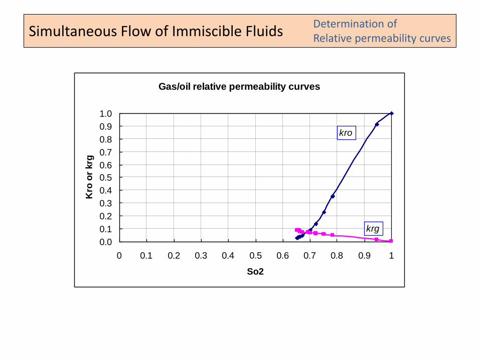
Gas/oil relative permeability curves
0.0
0.1
0.2
0.3
0.4
0.5
0.6
0.7
0.8
0.9
1.0
0 0.1 0.2 0.3 0.4 0.5 0.6 0.7 0.8 0.9 1
So2
Kro
or
krg
krg
kro
Simultaneous Flow of Immiscible Fluids
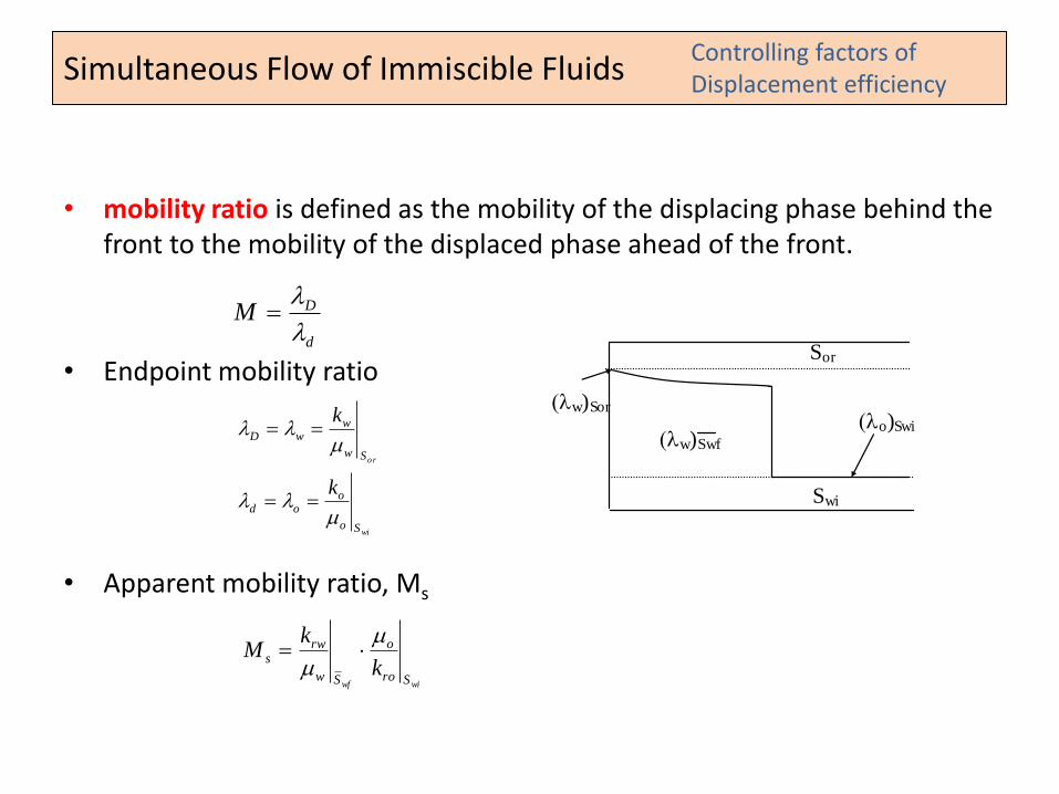
• mobility ratio is defined as the mobility of the displacing phase behind the front to the mobility of the displaced phase ahead of the front.
• Endpoint mobility ratio
• Apparent mobility ratio, Ms
Controlling factors of Displacement efficiency
Sor
Swi
w)Sor
w)Swf o)Swi
d
DM
wi
or
So
ood
Sw
wwD
k
k
wiwf Sro
o
Sw
rws
k
kM
Simultaneous Flow of Immiscible Fluids
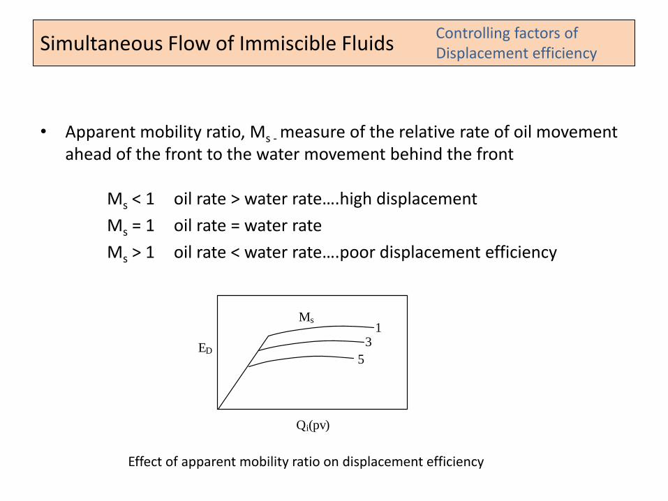
• Apparent mobility ratio, Ms - measure of the relative rate of oil movement ahead of the front to the water movement behind the front
Ms < 1 oil rate > water rate….high displacement
Ms = 1 oil rate = water rate
Ms > 1 oil rate < water rate….poor displacement efficiency
Controlling factors of Displacement efficiency
ED
Qi(pv)
Ms
3 1
5
Effect of apparent mobility ratio on displacement efficiency
Simultaneous Flow of Immiscible Fluids
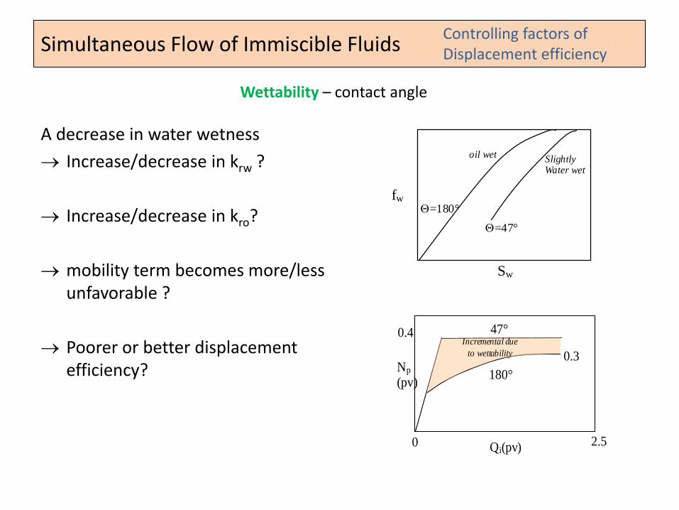
A decrease in water wetness
Increase/decrease in krw ?
Increase/decrease in kro?
mobility term becomes more/less unfavorable ?
Poorer or better displacement efficiency?
Controlling factors of Displacement efficiency
Sw
=47°
Slightly Water wet
fw
oil wet
=180°
Np
(pv)
Qi(pv)
47°
2.5
0.4
0
0.3
180°
Incremental due
to wettability
Wettability – contact angle
Simultaneous Flow of Immiscible Fluids
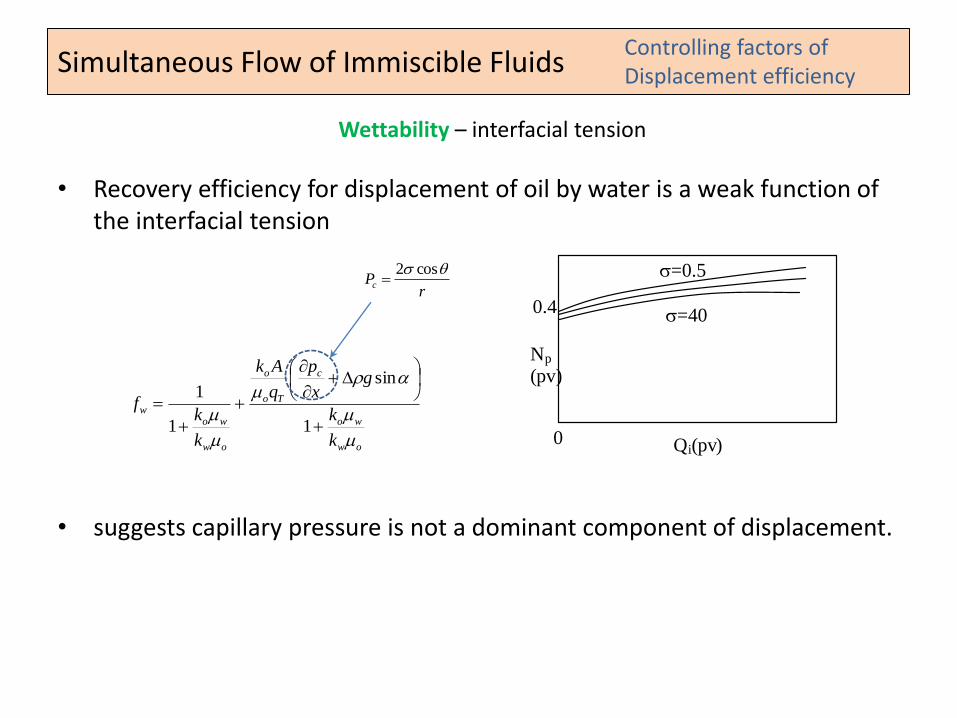
• Recovery efficiency for displacement of oil by water is a weak function of the interfacial tension
• suggests capillary pressure is not a dominant component of displacement.
Controlling factors of Displacement efficiency
Wettability – interfacial tension
Np
(pv)
Qi(pv)
=0.5
0.4
0
=40
ow
wo
c
To
o
ow
wow
k
k
gx
p
q
Ak
k
kf
1
sin
1
1
rPc
cos2
Simultaneous Flow of Immiscible Fluids Controlling factors of Displacement efficiency
Sw
o/w= fw
100 10 1
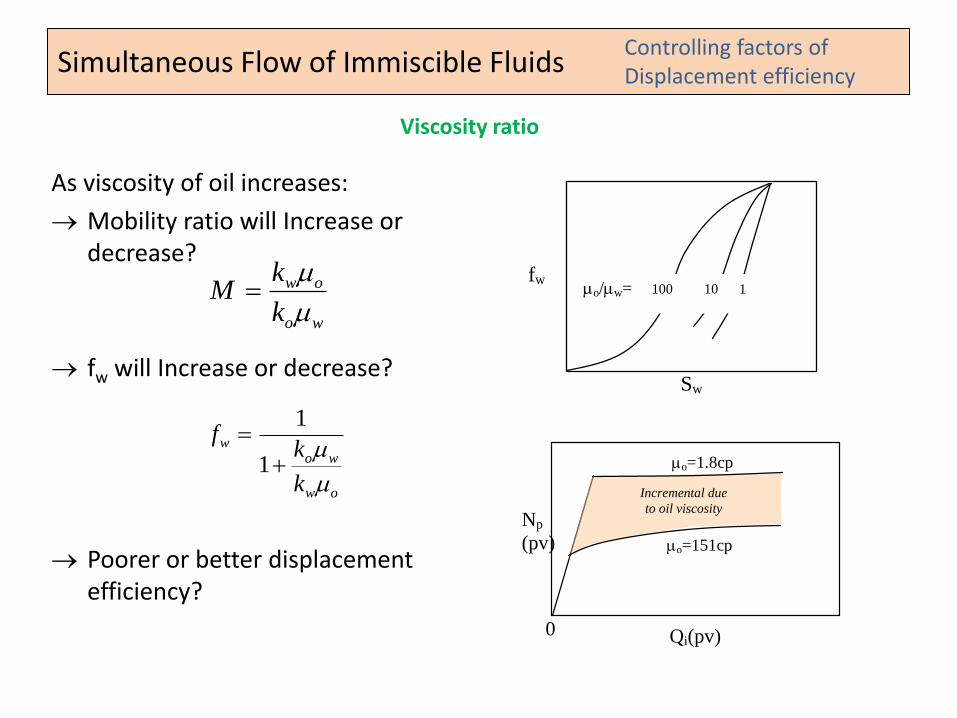
Viscosity ratio
Np
(pv)
Qi(pv)
o=1.8cp
0
Incremental due
to oil viscosity
o=151cp
wo
ow
k
kM
As viscosity of oil increases:
Mobility ratio will Increase or decrease?
fw will Increase or decrease?
Poorer or better displacement efficiency?
ow
wow
k
kf
1
1
Simultaneous Flow of Immiscible Fluids
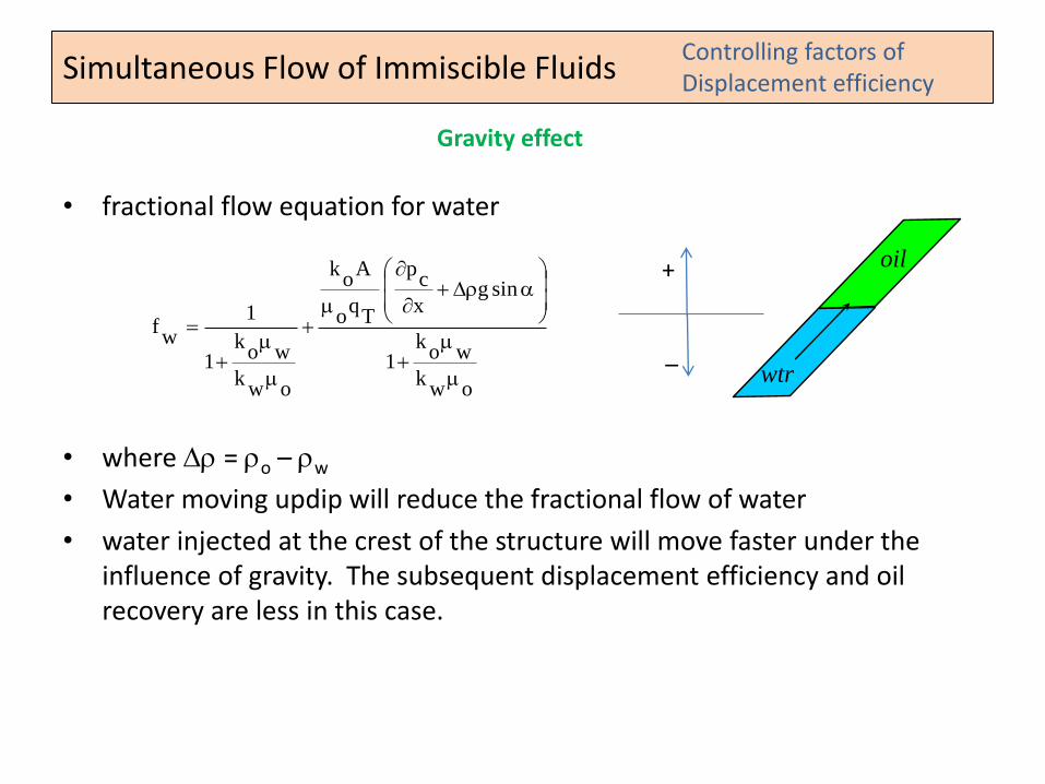
• fractional flow equation for water
• where = o – w
• Water moving updip will reduce the fractional flow of water
• water injected at the crest of the structure will move faster under the influence of gravity. The subsequent displacement efficiency and oil recovery are less in this case.
Controlling factors of Displacement efficiency
Gravity effect
wtr
oil
owk
wok
1
singx
cp
Tq
o
Ao
k
owk
wok
1
1w
f
+
_
Simultaneous Flow of Immiscible Fluids
• ROS is dependent upon: – Wettability
– Pore size distribution
– Hetergeneity
– Properties of displacing fluid
• Importance of ROS: – Establishes the maximum efficiency for the displacement of oil by water on a
microscopic level
– It is the initial saturation for EOR processes in regions of a reservoir previously swept by a waterflood
Controlling factors of Displacement efficiency
Residual Oil Saturation
Simultaneous Flow of Immiscible Fluids
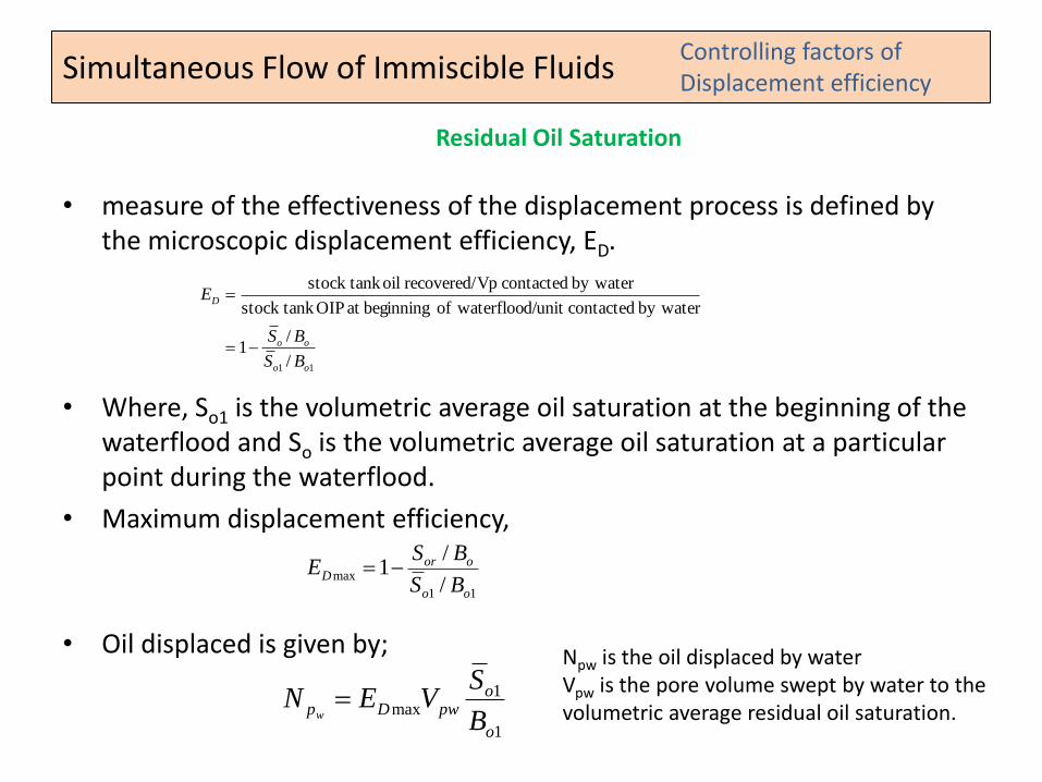
• measure of the effectiveness of the displacement process is defined by the microscopic displacement efficiency, ED.
• Where, So1 is the volumetric average oil saturation at the beginning of the waterflood and So is the volumetric average oil saturation at a particular point during the waterflood.
• Maximum displacement efficiency,
• Oil displaced is given by;
Controlling factors of Displacement efficiency
Residual Oil Saturation
11 /
/1
by water contactedd/unit waterflooof beginningat OIP stock tank
by water contacted Vprecovered/ oil stock tank
oo
oo
D
BS
BS
E
1
1max
o
opwDp
B
SVEN
w
11
max/
/1
oo
oorD
BS
BSE
Npw is the oil displaced by water Vpw is the pore volume swept by water to the volumetric average residual oil saturation.
Simultaneous Flow of Immiscible Fluids
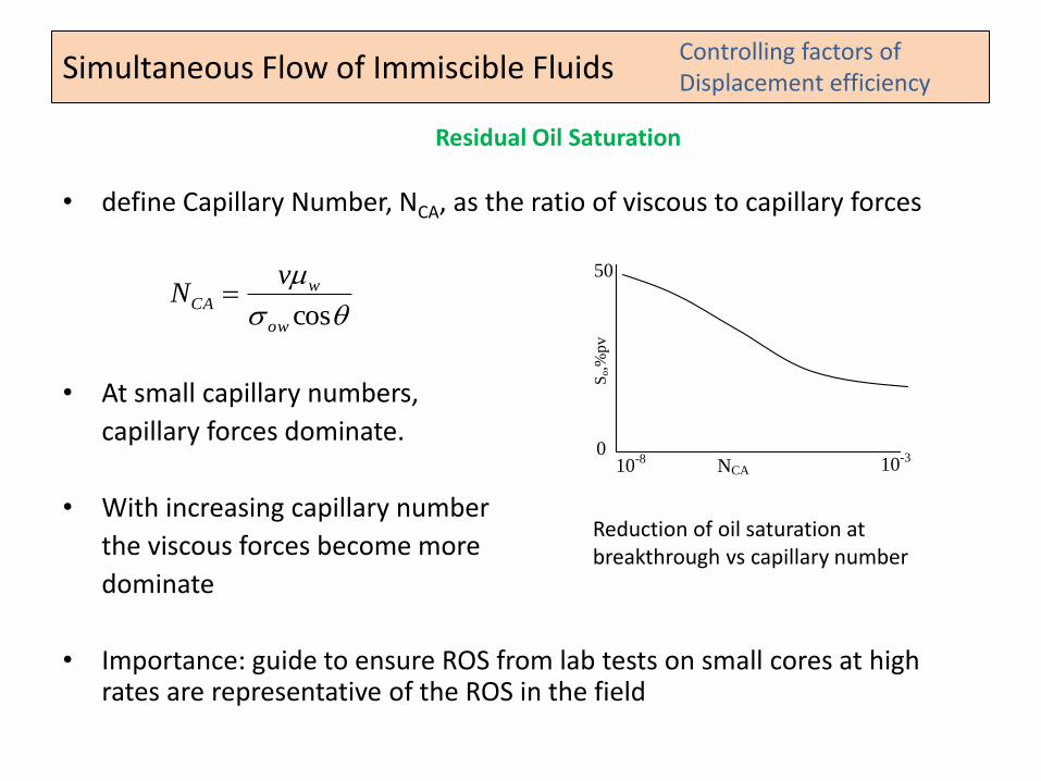
• define Capillary Number, NCA, as the ratio of viscous to capillary forces
• At small capillary numbers,
capillary forces dominate.
• With increasing capillary number
the viscous forces become more
dominate
• Importance: guide to ensure ROS from lab tests on small cores at high rates are representative of the ROS in the field
Controlling factors of Displacement efficiency
Residual Oil Saturation
cosow
wCA
vN
0 NCA 10
-8 10
-3
50
So,%
pv
Reduction of oil saturation at breakthrough vs capillary number
Simultaneous Flow of Immiscible Fluids
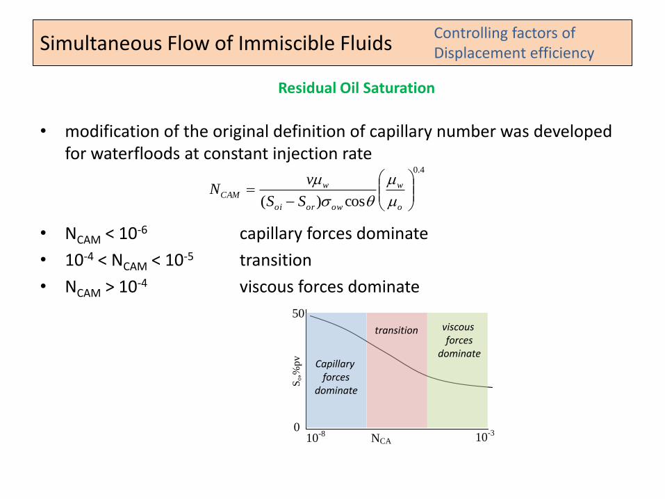
• modification of the original definition of capillary number was developed for waterfloods at constant injection rate
• NCAM < 10-6 capillary forces dominate
• 10-4 < NCAM < 10-5 transition
• NCAM > 10-4 viscous forces dominate
Controlling factors of Displacement efficiency
Residual Oil Saturation
4.0
cos)(
o
w
oworoi
wCAM
SS
vN
0 NCA 10
-8 10
-3
50
So,%
pv
Capillary forces
dominate
viscous forces
dominate
transition
Simultaneous Flow of Immiscible Fluids
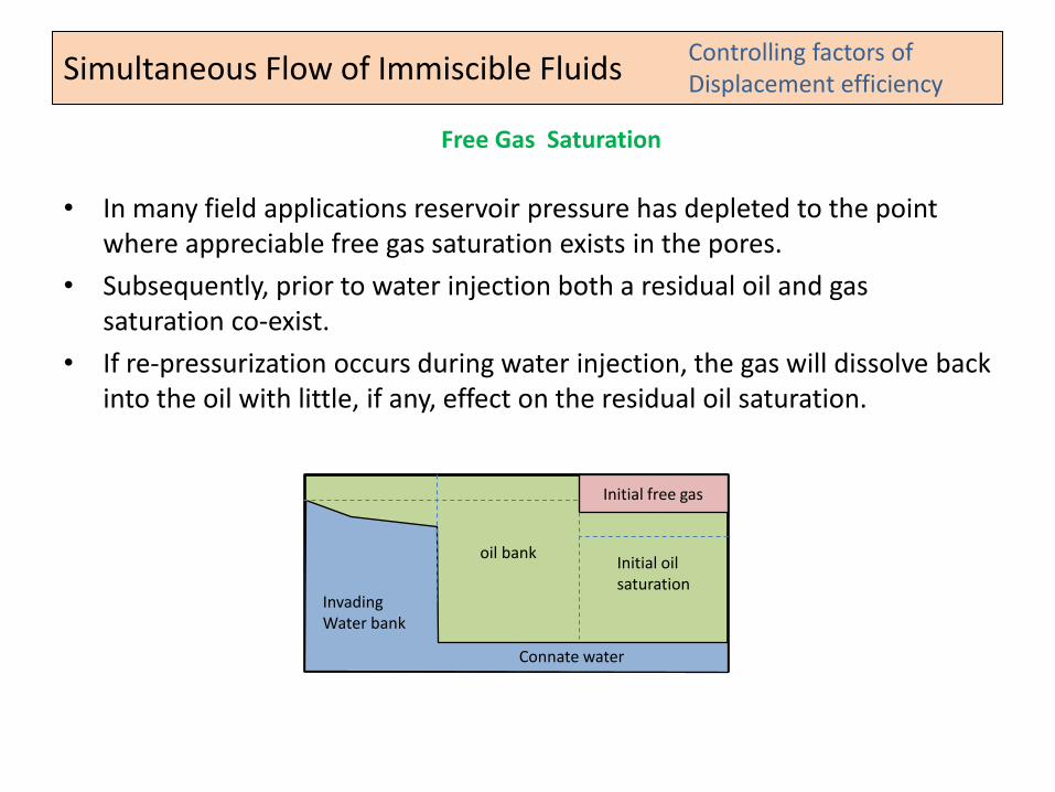
• In many field applications reservoir pressure has depleted to the point where appreciable free gas saturation exists in the pores.
• Subsequently, prior to water injection both a residual oil and gas saturation co-exist.
• If re-pressurization occurs during water injection, the gas will dissolve back into the oil with little, if any, effect on the residual oil saturation.
Controlling factors of Displacement efficiency
Free Gas Saturation
Invading Water bank
Connate water
Initial free gas
Initial oil saturation
oil bank
Simultaneous Flow of Immiscible Fluids
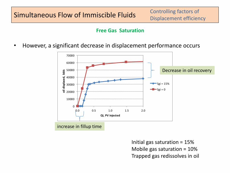
• However, a significant decrease in displacement performance occurs
Controlling factors of Displacement efficiency
Free Gas Saturation
0
10000
20000
30000
40000
50000
60000
70000
0.0 0.5 1.0 1.5 2.0
oil
dis
pla
ced
, b
bls
Qi, PV injected
Sgi = 15%
Sgi = 0
Decrease in oil recovery
increase in fillup time
Initial gas saturation = 15% Mobile gas saturation = 10% Trapped gas redissolves in oil
Simultaneous Flow of Immiscible Fluids
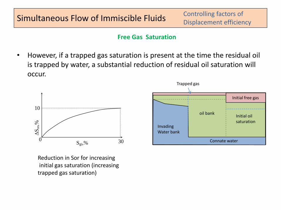
• However, if a trapped gas saturation is present at the time the residual oil is trapped by water, a substantial reduction of residual oil saturation will occur.
Controlling factors of Displacement efficiency
Free Gas Saturation
Sgi,%
10
0 30
S
or,%
Reduction in Sor for increasing initial gas saturation (increasing trapped gas saturation)
Invading Water bank
Connate water
Initial free gas
Initial oil saturation
oil bank
Trapped gas
Simultaneous Flow of Immiscible Fluids
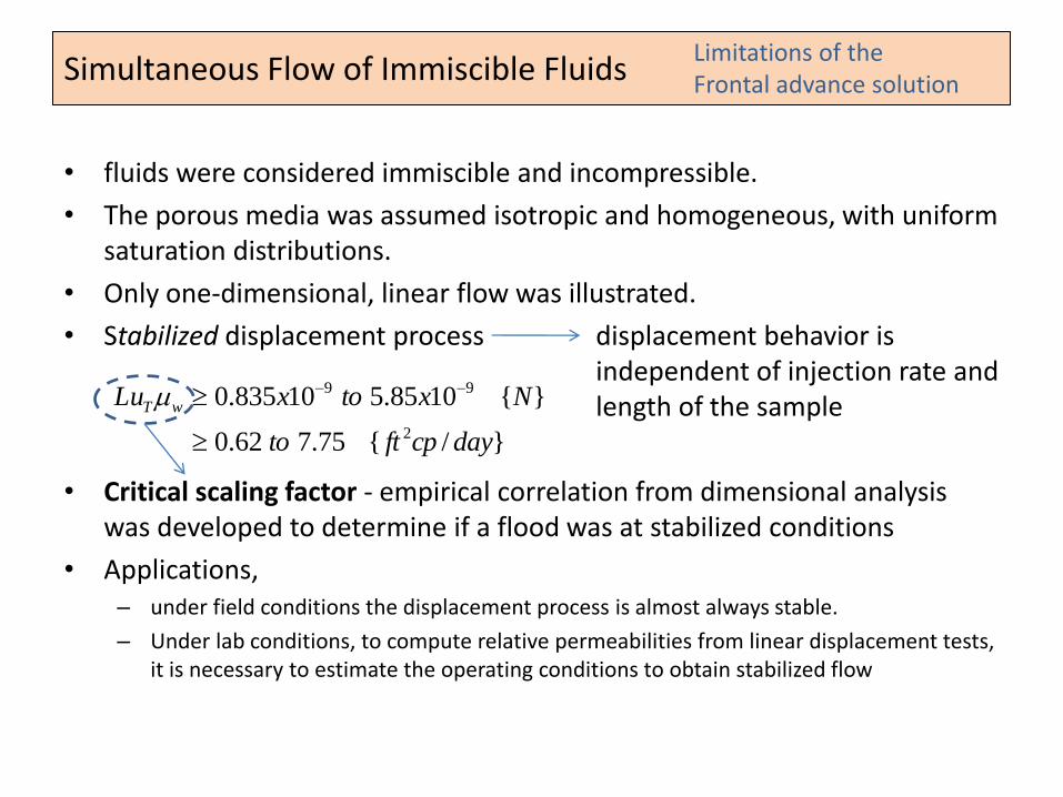
• fluids were considered immiscible and incompressible.
• The porous media was assumed isotropic and homogeneous, with uniform saturation distributions.
• Only one-dimensional, linear flow was illustrated.
• Stabilized displacement process displacement behavior is independent of injection rate and length of the sample
• Critical scaling factor - empirical correlation from dimensional analysis was developed to determine if a flood was at stabilized conditions
• Applications, – under field conditions the displacement process is almost always stable.
– Under lab conditions, to compute relative permeabilities from linear displacement tests, it is necessary to estimate the operating conditions to obtain stabilized flow
Limitations of the Frontal advance solution
}/{75.762.0
}{1085.510835.0
2
99
daycpftto
NxtoxLu wT
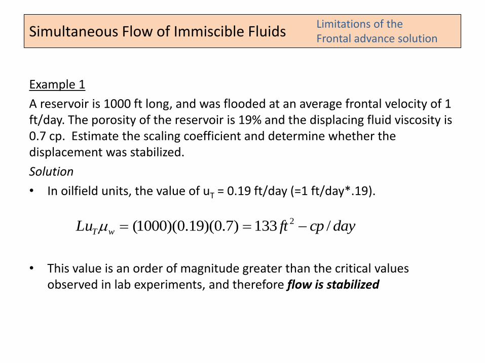
Simultaneous Flow of Immiscible Fluids
Example 1
A reservoir is 1000 ft long, and was flooded at an average frontal velocity of 1 ft/day. The porosity of the reservoir is 19% and the displacing fluid viscosity is 0.7 cp. Estimate the scaling coefficient and determine whether the displacement was stabilized.
Solution
• In oilfield units, the value of uT = 0.19 ft/day (=1 ft/day*.19).
• This value is an order of magnitude greater than the critical values observed in lab experiments, and therefore flow is stabilized
Limitations of the Frontal advance solution
daycpftLu wT /133)7.0)(19.0)(1000( 2
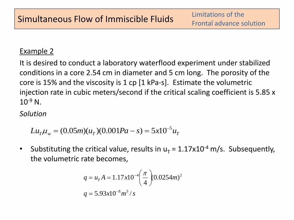
Simultaneous Flow of Immiscible Fluids
Example 2
It is desired to conduct a laboratory waterflood experiment under stabilized conditions in a core 2.54 cm in diameter and 5 cm long. The porosity of the core is 15% and the viscosity is 1 cp [1 kPa-s]. Estimate the volumetric injection rate in cubic meters/second if the critical scaling coefficient is 5.85 x 10⁻⁹ N.
Solution
• Substituting the critical value, results in uT = 1.17x10⁻⁴ m/s. Subsequently, the volumetric rate becomes,


![Viscoelastic Immiscible Double Layer Fluid Flow over ... › pdf › JAEBS › J. Appl. Environ...Later on Kapur et al. [8] discuss the flow of immiscible fluids between two plates](https://static.documents.pub/doc/80x56/60c5b1307b6f4638b529e93b/viscoelastic-immiscible-double-layer-fluid-flow-over-a-pdf-a-jaebs-a-j.jpg)


