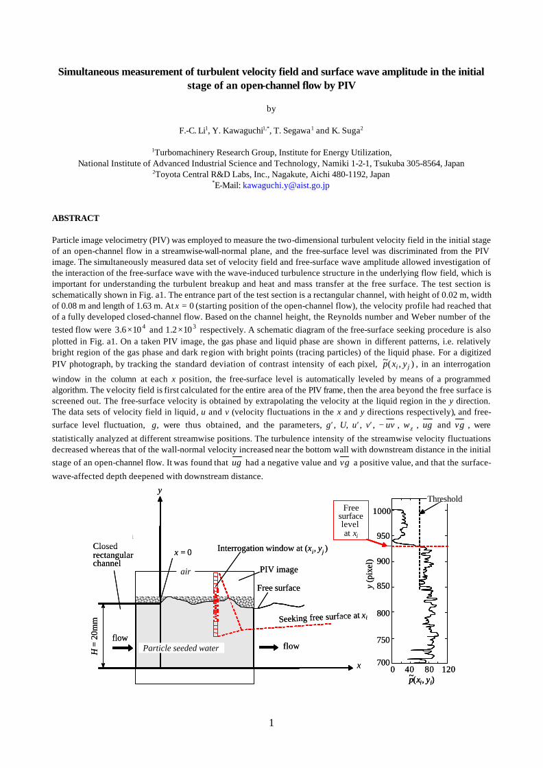
1 Simultaneous measurement of turbulent velocity field and surface wave amplitude in the initial stage of an open-channel flow by PIV by F.-C. Li 1 , Y. Kawaguchi 1,* , T. Segawa 1 and K. Suga 2 1 Turbomachinery Research Group, Institute for Energy Utilization, National Institute of Advanced Industrial Science and Technology, Namiki 1-2-1, Tsukuba 305-8564, Japan 2 Toyota Central R&D Labs, Inc., Nagakute, Aichi 480-1192, Japan * E-Mail: [email protected]ABSTRACT Particle image velocimetry (PIV) was employed to measure the two-dimensional turbulent velocity field in the initial stage of an open-channel flow in a streamwise-wall-normal plane, and the free-surface level was discriminated from the PIV image. The simultaneously measured data set of velocity field and free-surface wave amplitude allowed investigation of the interaction of the free-surface wave with the wave-induced turbulence structure in the underlying flow field, which is important for understanding the turbulent breakup and heat and mass transfer at the free surface. The test section is schematically shown in Fig. a1. The entrance part of the test section is a rectangular channel, with height of 0.02 m, width of 0.08 m and length of 1.63 m. At x = 0 (starting position of the open-channel flow), the velocity profile had reached that of a fully developed closed-channel flow. Based on the channel height, the Reynolds number and Weber number of the tested flow were 4 10 6 . 3 × and 3 10 2 . 1 × respectively. A schematic diagram of the free-surface seeking procedure is also plotted in Fig. a1. On a taken PIV image, the gas phase and liquid phase are shown in different patterns, i.e. relatively bright region of the gas phase and dark region with bright points (tracing particles) of the liquid phase. For a digitized PIV photograph, by tracking the standard deviation of contrast intensity of each pixel, ) , ( ~ j i y x p , in an interrogation window in the column at each x position, the free-surface level is automatically leveled by means of a programmed algorithm. The velocity field is first calculated for the entire area of the PIV frame, then the area beyond the free surface is screened out. The free-surface velocity is obtained by extrapolating the velocity at the liquid region in the y direction. The data sets of velocity field in liquid, u and v (velocity fluctuations in the x and y directions respectively), and free- surface level fluctuation, g, were thus obtained, and the parameters, g′ , U, u′ , v′ , uv - , z w , ug and vg , were statistically analyzed at different streamwise positions. The turbulence intensity of the streamwise velocity fluctuations decreased whereas that of the wall-normal velocity increased near the bottom wall with downstream distance in the initial stage of an open-channel flow. It was found that ug had a negative value and vg a positive value, and that the surface- wave-affected depth deepened with downstream distance. PIV image flow x y Run B Free surface H = 20mm Region B Closed rectangular channel x = 0 flow 700 750 800 850 900 950 1000 y (pixel) 0 40 80 120 p( x i , y j ) ~ Interrogation window at (x i , y j ) Seeking free surface at x i PIV image P1 P2 P3 P4 P5 P6 4.6 4.6 flow x y Run B Free surface H = 20mm Region B Closed rectangular channel x = 0 flow 700 750 800 850 900 950 1000 y (pixel) 0 40 80 120 p( x i , y j ) ~ p( x i , y j ) ~ Threshold Particle seeded water Interrogation window at (x i , y j ) Free surface level at x i Seeking free surface at x i air
Transcript
1
Simultaneous measurement of turbulent velocity field and surface wave amplitude in the initial stage of an open-channel flow by PIV
by
F.-C. Li1, Y. Kawaguchi1,*, T. Segawa1 and K. Suga2
1Turbomachinery Research Group, Institute for Energy Utilization, National Institute of Advanced Industrial Science and Technology, Namiki 1-2-1, Tsukuba 305-8564, Japan
2Toyota Central R&D Labs, Inc., Nagakute, Aichi 480-1192, Japan *E-Mail: [email protected]
ABSTRACT
Particle image velocimetry (PIV) was employed to measure the two-dimensional turbulent velocity field in the initial stage of an open-channel flow in a streamwise-wall-normal plane, and the free-surface level was discriminated from the PIV image. The simultaneously measured data set of velocity field and free-surface wave amplitude allowed investigation of the interaction of the free-surface wave with the wave-induced turbulence structure in the underlying flow field, which is important for understanding the turbulent breakup and heat and mass transfer at the free surface. The test section is schematically shown in Fig. a1. The entrance part of the test section is a rectangular channel, with height of 0.02 m, width of 0.08 m and length of 1.63 m. At x = 0 (starting position of the open-channel flow), the velocity profile had reached that of a fully developed closed-channel flow. Based on the channel height, the Reynolds number and Weber number of the tested flow were 4106.3 × and 3102.1 × respectively. A schematic diagram of the free-surface seeking procedure is also plotted in Fig. a1. On a taken PIV image, the gas phase and liquid phase are shown in different patterns, i.e. relatively bright region of the gas phase and dark region with bright points (tracing particles) of the liquid phase. For a digitized PIV photograph, by tracking the standard deviation of contrast intensity of each pixel, ),(~
ji yxp , in an interrogation
window in the column at each x position, the free-surface level is automatically leveled by means of a programmed algorithm. The velocity field is first calculated for the entire area of the PIV frame, then the area beyond the free surface is screened out. The free-surface velocity is obtained by extrapolating the velocity at the liquid region in the y direction. The data sets of velocity field in liquid, u and v (velocity fluctuations in the x and y directions respectively), and free-surface level fluctuation, g, were thus obtained, and the parameters, g′, U, u′, v′, uv− , zω , ug and vg , were
statistically analyzed at different streamwise positions. The turbulence intensity of the streamwise velocity fluctuations decreased whereas that of the wall-normal velocity increased near the bottom wall with downstream distance in the initial stage of an open-channel flow. It was found that ug had a negative value and vg a positive value, and that the surface-
wave-affected depth deepened with downstream distance.
PIV image
P1 P2 P3 P4 P5 P6
4.8 4.6 4.6 4.6 4.6 4.6 flow
x
y
Run B
Unit: mm
Free surface
H=
20m
m
Region B
Closed rectangularchannel
x = 0
flow
700
750
800
850
900
950
1000
y (p
ixel
)
0 40 80 120p(xi, yj)~
Threshold
Particle seeded water
Interrogation window at (xi, yj )
Freesurfacelevel at xi
Seeking free surface at xi
air PIV image
P1 P2 P3 P4 P5 P6
4.8 4.6 4.6 4.6 4.6 4.6 flow
x
y
Run B
Unit: mm
Free surface
H=
20m
m
Region B
Closed rectangularchannel
x = 0
flow
700
750
800
850
900
950
1000
y (p
ixel
)
0 40 80 120p(xi, yj)~p(xi, yj)~
Threshold
Particle seeded water
Interrogation window at (xi, yj )
Freesurfacelevel at xi
Seeking free surface at xi
air
2
Fig. a1 Schematic of flow, PIV image, coordinates system and free-surface tracking procedure
3
1. INTRODUCTION
Free-surface flow with interfacial transport processes is a subject of great interest since its effects can be seen both in nature and in practical devices, such as the air-sea interface, ship wakes, and chemical processes like gas-absorption equipment. While free-surface turbulence has been studied by many researchers, mo st of the investigations were limited to a free-surface flow with no shear or negligible surface deformation under shear and/or at low Reynolds numbers (Fulgosi et al. 2003, Kunugi et al. 2001, Kumar et al. 1998, Triantafyllou and Dimas 1989, Komori et al. 1982) due to the difficulty of measuring turbulent velocity close to a moving and deformed free surface in experimental studies and the impracticality today of performing direct numerical simulation of turbulent flow at moderate to high Reynolds numbers in numerical studies (Rashidi et al. 1992, Shi et al. 2000). For a free-surface flow with non-negligible surface deformation (wavy surface), there arise additional issues concerning the wave-turbulence interaction, and also the difficulty of measuring such flow since the investigation of wave-turbulence interaction requires simultaneous measurement of the turbulent velocity field and surface waves.
There have been very few experimental studies on a free-surface flow with significant deformed surface through simultaneously acquiring the velocity field and surface deformation compared with studies on a free-surface flow with no shear or negligible surface deformation. Rashidi et al. (1992) studied the wave-turbulence interaction in turbulent open-channel flow using microbubble tracers and visualization. Two cameras recording simultaneously were used in their study, one for viewing the wall structures and their interactions with the wavy interfaces and the other for recording the wave characteristics at the interface. They showed that the frequency of turbulent ejection occurring near the bottom wall increased as the surface wave amplitude increased, and that the wall shear stress increased under surface wave crests and diminished under wave troughs with the average remaining about the same as in the case with no surface waves. In the work of Dabiri and Gharib (2001), a free-surface flow with a vertical shear layer intersecting the free surface was investigated by simultaneously measuring the turbulent velocity field in a streamwise-spanwise plane near the free surface by digital particle image velocimetry (PIV) and the free-surface elevation with the reflective mode of the free-surface gradient detector technique. They found that the near-surface deformation best correlated with the near-surface normal-component-vorticity field. The laser specklegram method and stereo-PIV were used by Tanaka et al. (2002) to simultaneously measure the three-dimensional free-surface shape and three velocity components beneath the free surface, respectively, in order to investigate the interaction of a horizontal jet and free surface. They concluded that the vertical component of the jet had a strong effect on the free-surface waves.
In the present work, we report a simple but new non-intrusive approach for simultaneously measuring the free-surface level and turbulent velocity field beneath the surface for which no additional apparatus other than PIV is needed. The approach is described and demonstrated by measuring the correlations between the free-surface level and turbulent velocity in the liquid phase in the initial stage of an open-channel flow. PIV was used to measure the two-dimensional turbulent velocity field in a plane parallel to the streamwise direction and normal to the bottom wall, and the free-surface level was discriminated from the PIV image simultaneously. The interaction of the free-surface wave with the turbulence structure in the underlying flow field could thus be investigated, which is important for understanding the turbulent breakup and heat and mass transfer at the free surface at moderate to high Reynolds numbers.
2. EXPERIMENTAL METHOD AND PROCEDURES
2.1 Test Facility
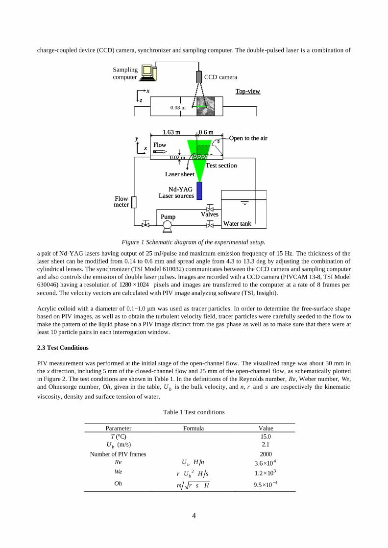
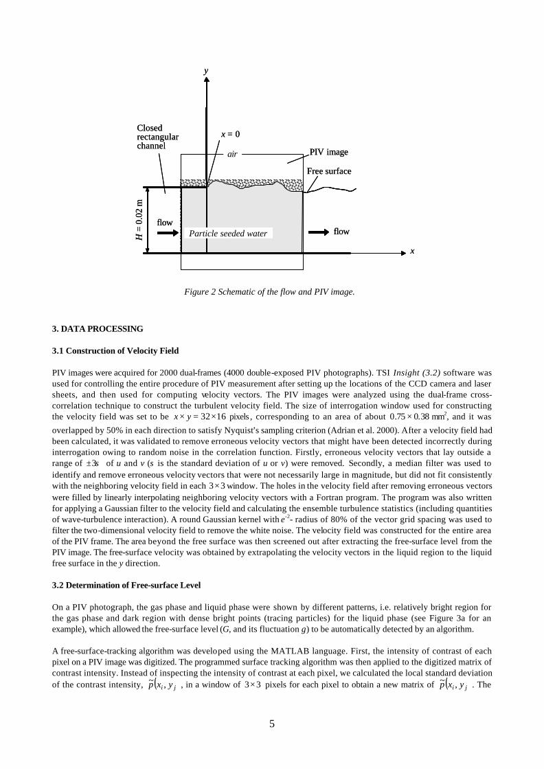
Figure 1 shows the experimental setup, composed of a circulating pump, electromagnetic flow meter, test section, water tank and pipelines and valves. The entrance part of the test section made of transparent acrylic resin is a closed rectangular channel with height (H) of 0.02 m, width of 0.08 m and length of 1.63 m; the latter part is an open channel with the same width and 0.6 m long. The starting position of the open channel (outlet of the closed channel) is located at 81.5H downstream from the channel inlet where the flow is fully developed for a Newtonian fluid. In the Cartesian coordinate system shown in Figure 1, x is the streamwise direction, y is normal to the bottom wall and z is the spanwise direction. Tap water was used as the working fluid.
2.2 PIV System
PIV was employed to simultaneously measure the deformed free-surface level and the turbulent velocity field of the liquid phase in the streamwise-wall-normal (x-y) plane. The PIV system included a double-pulsed laser, laser sheet optics,
4
charge-coupled device (CCD) camera, synchronizer and sampling computer. The double-pulsed laser is a combination of
a pair of Nd-YAG lasers having output of 25 mJ/pulse and maximum emission frequency of 15 Hz. The thickness of the laser sheet can be modified from 0.14 to 0.6 mm and spread angle from 4.3 to 13.3 deg by adjusting the combination of cylindrical lenses. The synchronizer (TSI Model 610032) communicates between the CCD camera and sampling computer and also controls the emission of double laser pulses. Images are recorded with a CCD camera (PIVCAM 13-8, TSI Model 630046) having a resolution of 10241280 × pixels and images are transferred to the computer at a rate of 8 frames per second. The velocity vectors are calculated with PIV image analyzing software (TSI, Insight).
Acrylic colloid with a diameter of 0.1−1.0 µm was used as tracer particles. In order to determine the free-surface shape based on PIV images, as well as to obtain the turbulent velocity field, tracer particles were carefully seeded to the flow to make the pattern of the liquid phase on a PIV image distinct from the gas phase as well as to make sure that there were at least 10 particle pairs in each interrogation window.
2.3 Test Conditions
PIV measurement was performed at the initial stage of the open-channel flow. The visualized range was about 30 mm in the x direction, including 5 mm of the closed-channel flow and 25 mm of the open-channel flow, as schematically plotted in Figure 2. The test conditions are shown in Table 1. In the definitions of the Reynolds number, Re, Weber number, We, and Ohnesorge number, Oh, given in the table, bU is the bulk velocity, and ν, ρ and σ are respectively the kinematic
viscosity, density and surface tension of water.
Table 1 Test conditions
Parameter Formula Value T (°C) 15.0
bU (m/s) 2.1
Number of PIV frames 2000 Re νHUb ⋅ 4106.3 × We σρ HUb ⋅⋅ 2 3102.1 ×
Oh H⋅⋅σρµ 4105.9 −×
Figure 1 Schematic diagram of the experimental setup.
Samplingcomputer
xz
x
y
0.02 m
CCD camera
Top-view
Flow
1.63 m 0.6 m
Pump
Flowmeter
Nd-YAG Laser sources
Valves
Test section
Open to the air
Water tank
Laser sheet
0.08 m
Samplingcomputer
xz
x
y
0.02 m
CCD camera
Top-view
Flow
1.63 m 0.6 m
Pump
Flowmeter
Nd-YAG Laser sources
Valves
Test section
Open to the air
Water tank
Laser sheet
0.08 m
Samplingcomputer
xz
x
y
0.02 m
CCD camera
Top-view
Flow
1.63 m 0.6 m
Pump
Flowmeter
Nd-YAG Laser sources
Valves
Test section
Open to the air
Water tank
Laser sheet
0.08 m
Samplingcomputer
xz
x
y
0.02 m
CCD camera
Top-view
Flow
1.63 m 0.6 m
Pump
Flowmeter
Nd-YAG Laser sources
Valves
Test section
Open to the air
Water tank
Laser sheet
0.08 m
5
3. DATA PROCESSING
3.1 Construction of Velocity Field
PIV images were acquired for 2000 dual-frames (4000 double-exposed PIV photographs). TSI Insight (3.2) software was used for controlling the entire procedure of PIV measurement after setting up the locations of the CCD camera and laser sheets, and then used for computing velocity vectors. The PIV images were analyzed using the dual-frame cross-correlation technique to construct the turbulent velocity field. The size of interrogation window used for constructing the velocity field was set to be 1632×=× yx pixels , corresponding to an area of about 38.075.0 × mm2, and it was
overlapped by 50% in each direction to satisfy Nyquist’s sampling criterion (Adrian et al. 2000). After a velocity field had been calculated, it was validated to remove erroneous velocity vectors that might have been detected incorrectly during interrogation owing to random noise in the correlation function. Firstly, erroneous velocity vectors that lay outside a range of σ3± of u and v (σ is the standard deviation of u or v) were removed. Secondly, a median filter was used to identify and remove erroneous velocity vectors that were not necessarily large in magnitude, but did not fit consistently with the neighboring velocity field in each 33× window. The holes in the velocity field after removing erroneous vectors were filled by linearly interpolating neighboring velocity vectors with a Fortran program. The program was also written for applying a Gaussian filter to the velocity field and calculating the ensemble turbulence statistics (including quantities of wave-turbulence interaction). A round Gaussian kernel with e-2- radius of 80% of the vector grid spacing was used to filter the two-dimensional velocity field to remove the white noise. The velocity field was constructed for the entire area of the PIV frame. The area beyond the free surface was then screened out after extracting the free-surface level from the PIV image. The free-surface velocity was obtained by extrapolating the velocity vectors in the liquid region to the liquid free surface in the y direction.
3.2 Determination of Free-surface Level
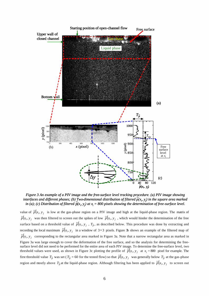
On a PIV photograph, the gas phase and liquid phase were shown by different patterns, i.e. relatively bright region for the gas phase and dark region with dense bright points (tracing particles) for the liquid phase (see Figure 3a for an example), which allowed the free-surface level (G, and its fluctuation g) to be automatically detected by an algorithm.
A free-surface-tracking algorithm was developed using the MATLAB language. First, the intensity of contrast of each pixel on a PIV image was digitized. The programmed surface tracking algorithm was then applied to the digitized matrix of contrast intensity. Instead of inspecting the intensity of contrast at each pixel, we calculated the local standard deviation of the contrast intensity, ( )ji yxp ,~ , in a window of 33× pixels for each pixel to obtain a new matrix of ( )ji yxp ,~ . The
Figure 2 Schematic of the flow and PIV image.
PIV image
P1 P2 P3 P4 P6
4.8 4.6 4.6 4.6 4.6 4.6 flow
x
y
Free surface
H=
0.02
mClosed rectangularchannel
x = 0
flowParticle seeded water
air PIV image
P1 P2 P3 P4 P6
4.8 4.6 4.6 4.6 4.6 4.6 flow
x
y
Free surface
H=
0.02
mClosed rectangularchannel
x = 0
flowParticle seeded water
air
6
value of ( )ji yxp ,~ is low at the gas-phase region on a PIV image and high at the liquid-phase region. The matrix of
( )ji yxp ,~ was then filtered to screen out the spikes of low ( )ji yxp ,~ , which would hinder the determination of the free
surface based on a threshold value of ( )ji yxp ,~ , pT~ , as described below. This procedure was done by extracting and
recording the local maximum ( )ji yxp ,~ in a window of 33× pixels. Figure 3b shows an example of the filtered map of
( )ji yxp ,~ corresponding to the rectangular area marked in Figure 3a. Note that a narrow rectangular area as marked in
Figure 3a was large enough to cover the deformation of the free surface, and so the analysis for determining the free-surface level did not need to be performed for the entire area of each PIV image. To determine the free-surface level, two threshold values were used, as shown in Figure 3c plotting the profile of ( )ji yxp ,~ at 800=ix pixel for example. The
first threshold value pT~ was set ( 60~ =pT for the tested flow) so that ( )ji yxp ,~ was generally below pT~ at the gas-phase
region and mostly above pT~ at the liquid-phase region. Although filtering has been applied to ( )ji yxp ,~ to screen out
(a)
Bottom wall
Upper wall ofclosed channel
Starting position of open-channel flow
Gas phase
Liquid phase
Free surface
(a)
Bottom wall
Upper wall ofclosed channel
Starting position of open-channel flow
(a)
Bottom wall
Upper wall ofclosed channel
Starting position of open-channel flow
Gas phase
Liquid phase
Free surface
x (pixel)
y(p
ixel
)
x (pixel)
y(p
ixel
)
(b)
(c)700
750
800
850
900
950
1000y
(pix
el)
0 40 80 120p(xi, yj)~p(xi, yj)~
Freesurfacelevel at xi
pT~
yT∆
(c)700
750
800
850
900
950
1000y
(pix
el)
0 40 80 120p(xi, yj)~p(xi, yj)~
Freesurfacelevel at xi
pT~pT~
yT∆
y∆y∆
Figure 3 An example of a PIV image and the free-surface level tracking procedure. (a) PIV image showing interfaces and different phases; (b) Two-dimensional distribution of filtered p(xi, yj) in the square area marked
in (a); (c) Distribution of filtered p(xi, yj) at xi = 800 pixels showing the determination of free-surface level.~~
7
the low-value spikes, points at which ( )ji yxp ,~ is lower than pT~ may still remain, which calls for the second threshold
value, yT∆ ( 20=∆yT pixels), as shown in Figure 3c. y∆ is the interval in which the points have the ( )ji yxp ,~ value
lower than pT~ and out of which ( )ji yxp ,~ values are larger than pT~ . Based on these two threshold values, the free-
surface level ( jy ) at ix satisfies the following constraints:
( ) pji Tyxp ~1 ,~ >− (1)
( ) ypkji TkTyxp ∆+ ⋅⋅⋅⋅⋅⋅=< , 2, ,1 , ,~ ~ (2)
The obtained profile of free-surface level at all the streamwise locations was then smoothed by using the zero-phase filter. The position of the bottom wall of the channel, upper wall of the closed channel and the starting point of the open-channel flow can be directly determined from the PIV image, as shown in Figure 3a. Figure 4a shows successful tracking of the free-surface level (blue curve) and the bottom wall, upper wall and position of the outlet of the closed channel (green lines). Note that the liquid surface of the open-channel flow was randomly deformed although the surface wave can be treated two-dimensionally in the x-y plane in a statistical sense. This random deformation of the liquid surface results in random reflection of the laser sheet at the free surface. In some frames, the reflection of laser light could contaminate the PIV image, causing extremely bright spots at the free surface and making the criteria for determining the free-surface level invalid, resulting in unusual representations of the profiles of the free-surface level as shown in Figure 4b for example. These frames with peculiar representations of the free-surface level were simply extracted and removed from the entire 2000 frames. Actually, the velocity field constructed at such spots with extremely high brightness caused by reflection of laser light was also significantly contaminated. In total, 163 contaminated frames were extracted from 2000 representations.
Figure 4 Examples of representations of tracking the free-surface level. 163 contaminated ones were found in 2000 representations.
3.3 Accuracy and resolution
By zooming-in the PIV image using Photoshop software, the number of pixels for each particle image appearing in the PIV image can be counted. In this way, about 3.9 pixels (91 µm) on average for each particle image were yielded for the present measurement. Prasad et al. (1992) showed that when particle images are well resolved so that the ratio of particle-image diameter pard to the size of a CCD pixel on the photograph pixd is 4~3>pixpar dd , the uncertainty of the
measurements is roughly one-tenth to one-twentieth of the particle-image diameter. This indicates that the particle images were adequately resolved for the present experiment, and the uncertainty in the measured displacement can be expected to be roughly less than one-tenth the diameter of the particle image, or about 9.1 µm. During the experiment, we judged the PIV image to be adequate based on a particle displacement of about 7 pixels on average by inspecting the same particle in the double images. Normalizing the uncertainty of measurement with this mean displacement of the particles (Adrian et al. 2000) yields a relative error of less than 5.6%.
(a) An example of a successful result (b) An example of a contaminated result
Contamination by random reflection of laser light
8
The spatial resolution of the velocity field is determined by the size of interrogation window. The interrogation area chosen for constructing the velocity field was about 38.075.0 × mm2 with 50% overlap in both directions, and so the spacing between adjacent velocity vectors was about 0.38 mm in the streamwise direction and 0.19 mm normal to the bottom wall. The spatial resolution of the free-surface level is similarly determined by the dimension of interrogation window used in the free-surface-level tracking algorithm. As described previously, first the local standard deviation of contrast intensity of each pixel on a PIV image was calculated and then ( )ji yxp ,~ was filtered in a 33× pixel window.
Hence, the spatial resolution of ( )ji yxp ,~ , which is directly associated with the spatial resolution of the free-surface level,
was 3 pixels or about 0.07 mm in either direction. Since the principal purpose of the simultaneous measurement of turbulent velocity field and the free-surface level was to investigate the free-surface wave-turbulence interaction, the data of free-surface level was also adjusted to fit the streamwise spacing between velocity vectors, so as to obtain the data sets of (u, g) and (v, g). Comparing the measured streamwise resolutions of g and u or v, 238.007.0 < , which
satisfies Nyquist’s sampling criterion when interpolating the data of g to fit the streamwise spacing of velocity vectors.
4. RESULTS AND DISCUSSION
Figure 5 plots an example of the processed PIV frame. The turbulent velocity field and its boundaries, solid wall and liquid free surface are simultaneously shown in the figure. The turbulence structures such as the coherent vortical structure near the bottom wall and its modification after released from the no-slip boundary condition near the free surface of the open-channel flow, and the evolvement of the free-surface wave can be seen from Figure 5. Statistical analyses of the measured turbulent velocity field and surface-level fluctuation are illustrated below. Note that to depict the evolvement of the turbulence structure and correlations between the turbulent velocity field and fluctuation of free-
Figure 5 An example of the processed PIV frame, including turbulent velocity field and the position of the wavy free surface.
10 20
0
5
10
15
20
25
2.62.32.01.71.41.20.90.60.30.0
x (mm)
y(m
m)
U (m/s)
Starting point of open channel flow
Free surface
Bottom wall
Upper wallof channel
10 20
0
5
10
15
20
25
2.62.32.01.71.41.20.90.60.30.0
x (mm)
y(m
m)
U (m/s)
Starting point of open channel flow
Free surface
Bottom wall
Upper wallof channel
0 0.5 1 1.50
0.01
0.02
x/H
g'/H
Figure 6 Fluctuation intensity of free-surface level.
9
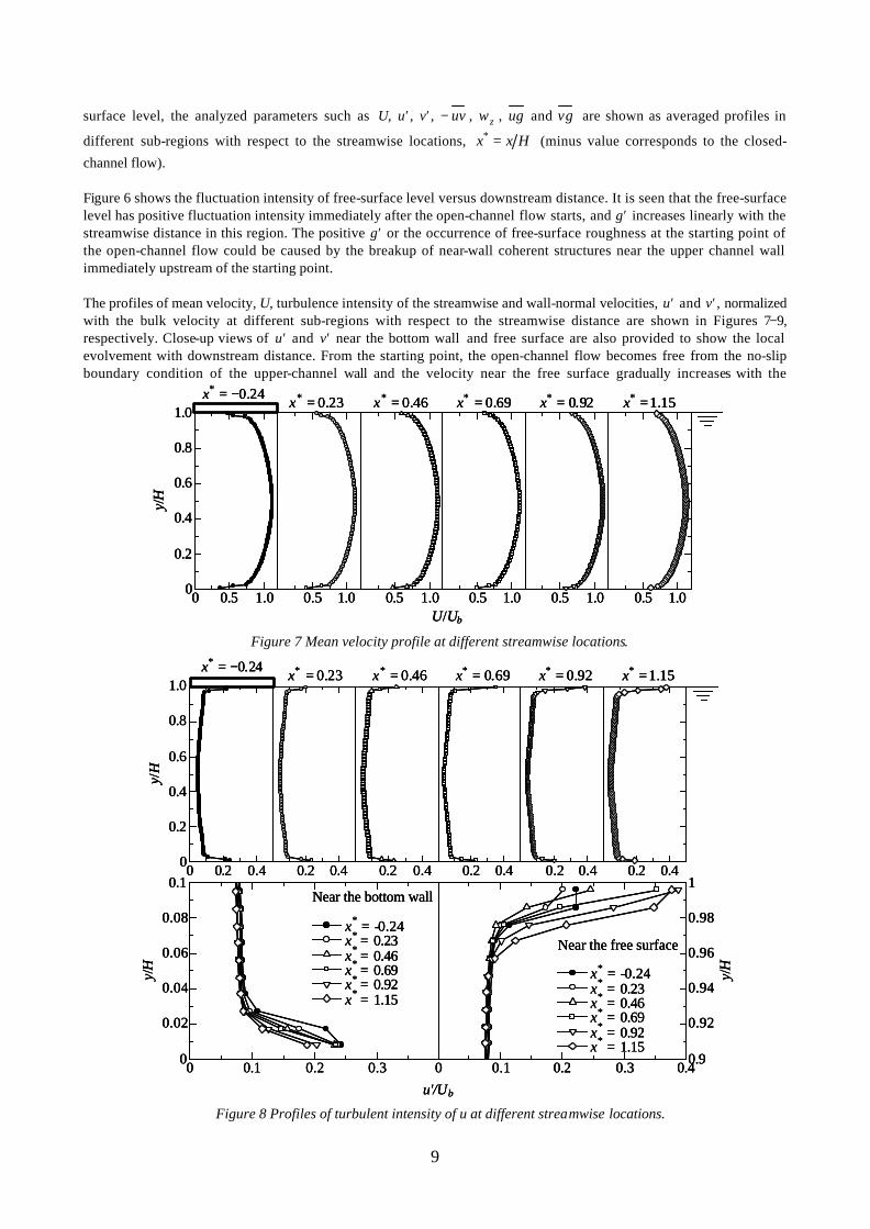
surface level, the analyzed parameters such as U, u′, v′, uv− , zω , ug and vg are shown as averaged profiles in
different sub-regions with respect to the streamwise locations, Hxx =* (minus value corresponds to the closed-
channel flow).
Figure 6 shows the fluctuation intensity of free-surface level versus downstream distance. It is seen that the free-surface level has positive fluctuation intensity immediately after the open-channel flow starts, and g′ increases linearly with the streamwise distance in this region. The positive g′ or the occurrence of free-surface roughness at the starting point of the open-channel flow could be caused by the breakup of near-wall coherent structures near the upper channel wall immediately upstream of the starting point.
The profiles of mean velocity, U, turbulence intensity of the streamwise and wall-normal velocities, u′ and v′, normalized with the bulk velocity at different sub-regions with respect to the streamwise distance are shown in Figures 7−9, respectively. Close-up views of u′ and v′ near the bottom wall and free surface are also provided to show the local evolvement with downstream distance. From the starting point, the open-channel flow becomes free from the no-slip boundary condition of the upper-channel wall and the velocity near the free surface gradually increases with the
Figure 7 Mean velocity profile at different streamwise locations.
streamwise distance (Figure 7). The turbulence intensity of the streamwise velocity near the free surface decreases in the immediate vicinity of the starting point of open-channel flow and then increases gradually with downstream location in the measured region (Figure 8). However, near the bottom wall, u′ monotonically decreases with the streamwise distance. Figure 9 shows that v′ increases near the bottom wall and then decreases in the bulk region when the flow moves downstream from the starting point of the open-channel flow. Near the free surface, the variance tendency of v′ is not clear. Figure 10 plots the dimensionless turbulent shear stress, 2
bUuv− , at different streamwise locations. Near the free
surface, 2bUuv− shows a decreasing tendency moving downward; near the bottom wall, the profile of 2
bUuv−
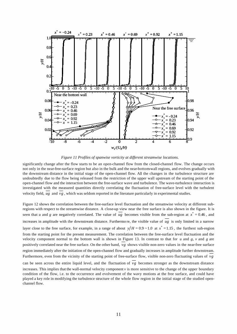
changes with the downstream distance without an obvious tendency. The spanwise vorticity, zω , calculated from the
two-dimensional velocity field in the x-y plane, is plotted in Figure 11 with close-up views near the bottom wall and liquid surface. It is clearly seen that the amplitude of vorticity gradually decreases both near the bottom wall and near the free surface with the streamwise distance, but the rate of decrease is higher near the free surface.
The phenomena appearing in the above-illustrated characteristic quantities indicate that the turbulence structures
Figure 9 Profiles of turbulent intensity of v at different streamwise locations.
significantly change after the flow starts to be an open-channel flow from the closed-channel flow. The change occurs not only in the near-free-surface region but also in the bulk and the near-bottom-wall regions, and evolves gradually with the downstream distance in the initial stage of the open-channel flow. All the changes in the turbulence structure are undoubtedly due to the flow being released from the restriction of the upper wall upstream of the starting point of the open-channel flow and the interaction between the free-surface wave and turbulence. The wave-turbulence interaction is investigated with the measured quantities directly correlating the fluctuation of free-surface level with the turbulent velocity field, ug and vg , which was seldom reported in the literature particularly in experimental studies.
Figure 12 shows the correlation between the free-surface level fluctuation and the streamwise velocity at different sub-regions with respect to the streamwise distance. A close-up view near the free surface is also shown in the figure. It is seen that u and g are negatively correlated. The value of ug becomes visible from the sub-region at 46.0* =x , and
increases in amplitude with the downstream distance. Furthermo re, the visible value of ug is only limited in a narrow
layer close to the free surface, for example, in a range of about 0.1~9.0=Hy at 15.1* =x , the furthest sub-region
from the starting point for the present measurement. The correlation between the free-surface level fluctuation and the velocity component normal to the bottom wall is shown in Figure 13. In contrast to that for u and g, v and g are positively correlated near the free surface. On the other hand, vg shows visible non-zero values in the near-free surface
region immediately after the initiation of the open-channel flow and gradually increases in amplitude further downstream. Furthermore, even from the vicinity of the starting point of free-surface flow, visible non-zero fluctuating values of vg
can be seen across the entire liquid level, and the fluctuation of vg becomes stronger as the downstream distance
increases. This implies that the wall-normal velocity component v is more sensitive to the change of the upper boundary condition of the flow, i.e. to the occurrence and evolvement of the wavy motions at the free surface, and could have played a key role in modifying the turbulence structure of the whole flow region in the initial stage of the studied open-channel flow.
Figure 11 Profiles of spanwise vorticity at different streamwise locations.
A simple but new experimental technique for simultaneously measuring the free-surface level and turbulent velocity field beneath the surface was presented, which employs a PIV system only to obtain the two-dimensional velocity field in a plane intersecting the liquid free surface while tracing the liquid surface from the PIV image. This technique was used to study the wave-turbulence interaction and the wave-induced turbulence structure in the initial stage of an open-channel flow by making PIV measurements in a plane parallel to the streamwise direction and normal to the channel bottom wall. Since it constructs the turbulent velocity field crossing the entire liquid level and profile of the wavy liquid free-surface over the velocity field, the technique provides an effective tool for investigating the wave phenomenon on the liquid surface, turbulence structures near both the bottom wall and free surface and wave-turbulence interaction. Preliminary results showed that the upstream no-slip boundary condition of the open-channel flow causes an immediate occurrence of the free-surface roughness. The measured turbulence statistics revealed that the turbulence structures in the entire flow region are modified from the start of free-surface flow and with the evolvement of free-surface waves. Near the free
13
surface, the free-surface level fluctuation is negatively correlated with the streamwise turbulent velocity whereas it is positively correlated with the velocity component normal to the bottom wall. It appears that the wall-normal turbulent velocity is more sensitive to the occurrence and evolvement of the free-surface waves.
ACKNOWLEDGMENT
The authors would like to thank Dr. N. Hutchins, Department of Aerospace Engineering and Mechanics, University of Minnesota, for his help in MATLAB programming of the algorithm of free-surface detection.
REFERENCES
Adrian, R.J., Meinhart C.D. and Tomkins, C.D. (2000) “Vortex Organization in the Outer Region of the Turbulent Boundary Layer”, J. Fluid Mech. 422, 1-54.
Dabiri, D. and Gharib, M. (2001) “Simultaneous Free-surface Deformation and Near-surface Velocity Measurements”, Exp. Fluids 30, 381-390.
Komori, S., Ueda, H., Ogino, F. and Mizushina, T. (1982) “Turbulence Structure and Transport Mechanism at the Free Surface in an Open Channel Flow”, Int. J. Heat Mass Transfer 25(4), 513-522.
Fulgosi, M., Lakehal, D., Banerjee, S. and De Angelis, V. (2003) “Direct Numerical Simulation of Turbulence in a Sheared Air-water Flow with a Deformable Interface”, J. Fluid Mech. 482, 319-345.
Kumar, S., Gupta, R. and Banerjee, S. (1998) “An Experimental Investigation of the Characteristics of Free-surface Turbulence in Channel Flow”, Phys. Fluids 10(2), 437-456.
Kunugi, T., Satake, S. and Ose, Y. (2001) “Direct Numerical Simulation of Carbon-dioxide Gas Absorption Caused by Turbulent Free-surface Flow”, Int. J. Heat Fluid Flow 22, 245-251.
Prasad, A.K., Adrian, R.J., Landreth, C.C. and Offutt, P.W. (1992) “Effect of Resolution on the Speed and Accuracy of Particle Image Velocimetry Interrogation”, Exp. Fluids 13, 105-116.
Rashidi, M., Hetsroni, G. and Banerjee, S. (1992) “Wave-turbulence Interaction in Free-surface Channel Flows”, Phys. Fluids A4(12), 2727-2738.
Shi, J., Thomas, T.G. and Williams, J.J.R. (2000) “Free-surface Effects in Open Channel Flow at Moderate Froude and Reynolds Numbers”, J. Hydraulic Res. 38(6), 465-474.
Tanaka, G., Ishitsu, Y., Okamoto, K. and Madarame, H. (2002) “Simultaneous Measurements of Free-surface and Turbulence Interaction Using Specklegram Method and Stereo-PIV”, Proc. 11th Int. Symp. App. Laser Tech. Fluid Mech., Lisbon, Portugal.
Triantafyllou, G.S. and Dimas, A.A. (1989) “Interaction of Two-dimensional Separated Flows with a Free Surface at Low Froude Numbers”, Phys. Fluids A1(11), 1813-1821.