Wright State University Wright State University CORE Scholar CORE Scholar Browse all Theses and Dissertations Theses and Dissertations 2008 Simultaneous RF/EO Tracking and Characterization of Dismounts Simultaneous RF/EO Tracking and Characterization of Dismounts Jason M. Blackaby Wright State University Follow this and additional works at: https://corescholar.libraries.wright.edu/etd_all Part of the Electrical and Computer Engineering Commons Repository Citation Repository Citation Blackaby, Jason M., "Simultaneous RF/EO Tracking and Characterization of Dismounts" (2008). Browse all Theses and Dissertations. 829. https://corescholar.libraries.wright.edu/etd_all/829 This Thesis is brought to you for free and open access by the Theses and Dissertations at CORE Scholar. It has been accepted for inclusion in Browse all Theses and Dissertations by an authorized administrator of CORE Scholar. For more information, please contact [email protected].
Transcript
Wright State University Wright State University
CORE Scholar CORE Scholar
Browse all Theses and Dissertations Theses and Dissertations
2008
Simultaneous RF/EO Tracking and Characterization of Dismounts Simultaneous RF/EO Tracking and Characterization of Dismounts
Jason M. Blackaby Wright State University
Follow this and additional works at: https://corescholar.libraries.wright.edu/etd_all
Part of the Electrical and Computer Engineering Commons
Repository Citation Repository Citation Blackaby, Jason M., "Simultaneous RF/EO Tracking and Characterization of Dismounts" (2008). Browse all Theses and Dissertations. 829. https://corescholar.libraries.wright.edu/etd_all/829
This Thesis is brought to you for free and open access by the Theses and Dissertations at CORE Scholar. It has been accepted for inclusion in Browse all Theses and Dissertations by an authorized administrator of CORE Scholar. For more information, please contact [email protected].
SIMULTANEOUS RF/EO TRACKINGAND CHARACTERIZATION OF
DISMOUNTS
A thesis submitted in partial fulfillmentof the requirements for the degree of
Master of Science in Engineering
by
JASON M. BLACKABYDepartment of Electrical Engineering
Wright State University
2008Wright State University
WRIGHT STATE UNIVERSITY
SCHOOL OF GRADUATE STUDIES
May 27, 2008
I HEREBY RECOMMEND THAT THE THESIS PREPARED UNDER MY SU-PERVISION BY Jason M. Blackaby ENTITLED Simultaneous RF/EO Tracking andCharacterization of Dismounts BE ACCEPTED IN PARTIAL FULFILLMENT OFTHE REQUIREMENTS FOR THE DEGREE OF Master of Science in Engineering.
Brian D. Rigling, Ph.D.Thesis Director
Fred Garber, Ph.D.Department Chair
Committee onFinal Examination
Brian D. Rigling, Ph.D.
Fred Garber, Ph.D.
Xiaodong Zhang, Ph.D.
Joseph F. Thomas, Jr., Ph.D.Dean, School of Graduate Studies
ABSTRACT
Blackaby, Jason M. M.S. Egr., Department of Electrical Engineering, 2008.Simultaneous RF/EO Tracking and Characterization of Dismounts.
This thesis discusses the fusion of radar frequency(RF) data and electro-optical
(EO) data for tracking and characterization of dismounts (i.e., humans). Each of
these sensor modalities provides unique information about the location, structure,
and movement of a dismount. The person’s location is tracked on the 2D ground
plane using RF data for range measurements and EO data for angle measurements.
Using this information, measurements are made on the structure and dynamic motion
(gait) of the person. An imaging approach is used to create spatio-temporal activity
maps along with a three-dimensional reconstruction of the dismount.
I would first like to think my advisor, Brian Rigling, for all of his help and direc-
tion. I would like to thank the Air Force Research Laboratory’s Sensors Directorate,
Automatic Target Recognition Division (AFRL/RYA) for funding this research. I
would like to individually thank William Pierson, formerly AFRL; Kyle Erickson,
AFRL; Philip Hanna, AFRL; Gregory Arnold, AFRL; and Erik Blasch, AFRL for
their technical input as well as their help with administrative tasks. Finally, I would
like to thank my family for all of their help and support.
viii
CHAPTER 1
INTRODUCTION
Remote sensing and characterization of articulated humans undergoing movement
is a fairly new and challenging task. While remote sensing of large rigid objects, such
as aircraft and ground vehicles has existed for some time, the continuing advancement
in digital computing in recent years has thrust remote sensing into new areas. Ar-
ticulated human motion presents a number of new challenges that do not exist with
large rigid objects.
Specifically, humans are smaller relative to the objects largely sensed in the past,
thus requiring finer sensor resolution. Humans are made up of an articulated struc-
ture with a range of possible poses, while most recongnition algorithms are heavily
dependent on shape. Humans can perform a wide range of motions making them dif-
ficult to model. A vehicle generally moves forward or backward at a variable velocity,
where a human can change directions quickly at any time. Human sensing often must
be done in the presence of significant structural clutter (e.g. buildings, trees, etc.).
Apart from dense urban environments, clutter is less of a problem in vehicle sensing.
1.1 Previous Work
Dismount tracking and characterization has received much attention in recent
years. With the advancement in computing power, real-time video processing for
human tracking has become possible. A number of studies have looked at the viability
of using human gait as a biometric. Studies have shown that human observers can
1
2
recognize people and their gender by gait [1][2][3]. The problem of automating this
process has been the subject of much research in the areas of signal processing and
automatic target recognition. Visual information from EO sensors is the basis for
most automated human characterization methods. In most cases, the background of
a video sequence is removed leaving just pixels on the person. The resulting binary
silhouette and its dynamics is input to a classification or recognition algorithm. The
authors of [4] provide a good overview of the state of the art in human gait recognition
using EO sensors.
While sensing humans with EO sensors is well developed, RF human sensing is
relatively new. Time-frequency analysis of micro-Doppler signatures has been exam-
ined [5][6]. Independent component analysis of micro-Doppler signatures has been
used to characterize the human gait [7]. Others have looked at the micro-Doppler
phenomenon in general [8][9][10]. The authors of [11] used a human walking model
to simulate radar signatures and estimate walking parameters from radar data. A
simple detector for dismounts using a continuous wave radar was developed in [12].
Some have looked at challenges for ISAR imaging in the presence of micro-Doppler
by separating micro-Doppler returns from those from the gross target motion [13][14].
1.2 Outline
This paper considers new methods to characterize humans as they move through
a scene. Measured radio-frequency and passive electro-optical sensor dismount data
is used as demonstration. A non-scanning, wide angle RF sensor provides good reso-
lution along the range dimension, but little or no resolution in azimuth or elevation.
Conversely, an EO sensor provides resolution in the azimuth and elevation dimen-
sions, but little or no resolution in range. By fusing information from both sensors,
the dismount can be resolved in azimuth, elevation, and range, which in turn can be
mapped to the x, y, z Cartesian space.
3
Some processing is required before a dismount can be imaged. The RF data
contains a large amount of ground clutter that is removed using a standard moving
target indicator (MTI) filter. The person is segmented in the video using background
and shadow subtraction techniques. The quality of the segmentation is a key part
of the process since much of the tracking and imaging is directly based upon it.
With the dismount returns isolated in both sensor domains, position measurements
are made and registered in time and space. The dismount position is tracked using
an extended kalman filter (EKF). The tracking information is used for dismount
motion compensation. With the gross motion of the dismount removed, some imaging
techniques can be employed. RF activity maps capture the micro-motion, motion
apart from the gross dismount motion (i.e., arms and legs) of the dismount in a
single image. Tomography is used to form a 3-D reconstruction of the dismount. EO
tomosynthesis and RF back-projection are performed on the motion-compensated
sensor data to form a 3-D map of the dismount.
The remainder of this paper is outlined as follows. Chapter 2 explains the mea-
sured data set and the data models for each sensor modality. Chapter 3 discusses the
suppression of background and non-dismount sensor returns. Chapter 4 describes a
joint RF/EO dismount tracking system. Chapter 5 explains the creation of spatio-
temporal activity maps to capture the nature of dismount motion in a single image.
Chapter 6 discusses 3-D imaging techniques for each sensor modality and their fusion
to form dismount images.
CHAPTER 2
MEASURED DATA SET
The data used in this study is unique in that it contains fine resolution radar and
video measurements of a number of dismount scenarios. The radar is a coherent,
pulse-Doppler radar operating in the X (fc = 10 GHz) and Ku (fc = 15 GHz) bands.
The radar has a pulse repetition frequency (PRF) of 1000 Hz and a bandwidth of
4 GHz, giving a range resolution of 1.48 inches. This is important for dismount
characterization as the motion of the arms and legs can be resolved from the torso.
The radar has a beamwidth of roughly 45◦, so it provides very little angle resolution.
Figure 2.1 shows the geometry of the scene in the data collection. The radar was
fourteen feet above the ground, which produces the positive effect of separating the
dismount returns from head to feet in range.
The EO data was captured with a standard NTSC camera with 720x480 pixel
resolution at 30 frames per second. The camera was situated directly below the radar
antenna, about five feet above the ground. The camera parameters were unknown
and were estimated based on known positions in the scene.
A number of scenarios are contained in the data, including dismounts walking,
jogging, running, carrying, standing, and limping. These actions are performed along
various paths relative to the sensor platform. RF and EO data were captured simul-
taneously and can be easily registered in time.
4
5
Sensor Platform
8.23 m
1.70 m0.15 m
2.37 m
3.18 m
2.92 m
2.67 m
5.84 m
0.03
X
Y
5.13 m
27.4° 55.6°
2.92 m
4.27 m
1.52 m
RF
EO
Y
Z
Figure 2.1: Data Collection Setup. This figure denotes the ground truth dimen-sions of the measured data set. The dismounts followed pre-defined paths on theground plane. The RF and EO sensors were located in the same location, but atdifferent heights. Note that the ground truth is not drawn to scale as the star patternis not symmetric.
2.1 EO Data Model
A basic EO system projects points in 3-D space onto a 2-D image surface. Figure
2.2 illustrates the projective camera geometry and image formation. Let γ represent
a point in 3-D space and γ represent the corresponding projected point on the focal
plane. The 3-D point is projected onto the focal plane by the projective camera
matrix P,
γ = Pγ (2.1)
6
u
vf
Z
X Y
Image Plane
Figure 2.2: Projective Camera Geometry. This figure shows the projective EOsystem geometry with respect to camera center c. The line formed by the cameracenter and the point γ intersects the image plane at the point γ.
where P is a 3×4 projection matrix determined by the camera characteristics, position,
and orientation. A homogenous coordinate system is used such that
γ =
X
Y
Z
1
and γ =
U
V
1
(2.2)
The common pinhole camera assumption is made in which the camera is represented
by a single point, c, in 3-D space. Any point, γ, and c form a line containing the
points [15]
γ(λ) = λγ + (1− λ)c (2.3)
As λ varies, γ(λ) traverses the line formed by γ and c. One point on this line will occur
at the intersection of the image plane with the line. This point, γ is the projected
point on the 2-D image image plane of all other points on the line, γ(λ), so (2.1) can
7
be extended to
γ = Pγ(λ) (2.4)
This indicates that in a perspective EO system, each 2-D image point can be the
projection of any point along a line in 3-D space. Consequently, the 3-D point cor-
responding to an image point cannot be determined completely by the image point.
However, an image point does provide the azimuth(φ) and elevation(θ) angle of the 3-
D ray on which the corresponding 3-D point lies if the camera parameters are known.
We define
φ(U) = arctanU
f(2.5a)
θ(V ) = arctanV
f(2.5b)
where U and V are the coordinates on the image plane with (U, V ) = (0, 0) at the
center of the image. The variable f is the focal length of the camera lens. The focal
length and the image size may not be known in many instances, but φ and θ can
also be determined from the field of view of the camera as well. The field of view
is given by the horizontal (Φ) and vertical (Θ) angles covered by the extents of the
image. The field of view is defined completely by the focal length and image size,
but the focal length and image size cannot necessarily be retrieved from the field of
view. The field of view can be estimated much easier than the focal length. If the
dimensions and range of an object in the scene are known, the field of view can be
estimated. However, determining the focal length usually requires calibration based
on a complex object such as a checkerboard cube. Assuming there is no skew or
8
distortion in the image, φ and θ linearly span Φ and Θ.
φ(U) =U
LUΦ (2.6a)
θ(V ) =V
LVΘ (2.6b)
where LU and LV are the horizontal and vertical lengths of the image plane. The
value of this representation can be seen in the digital image domain. Let u and v
represent the horizontal and vertical pixel indexes with (u, v) = (0, 0) occuring at the
center of the image. In this case, φ and θ are determined by
φ(u) =u
Nu
Φ (2.7a)
θ(v) =v
Nv
Θ (2.7b)
where Nu and Nv are the number of horizontal and vertical pixels respectively. This
indicates that knowledge of the field of view of the camera allows us to determine
the projection angles for each pixel in a digital image without additional information.
Knowledge of the projection angles is key to the dismount tracking process in Chapter
4 and the back-projection of γ to γ(λ) used in the tomosynthesis process discussed
in Chapter 6.
2.1.1 RF Data Model
A pulse Doppler radar generally consists of a transmitter that radiates an electro-
magnetic wave and a receiver that captures the reflections from objects in a scene. In
the monostatic case, the transmitter and receiver are in the same location and usually
share the same antenna. Many transmission waveforms are used in radar systems,
depending on the application.
For the measured data in this study, a stepped frequency system was employed,
9
resulting in measured returns well-modeled by
S(fi, τk) =∑m
Am exp
[−j2πfi
2Rm(τk)
c
](2.8)
where τk represents the time of the kth pulse, Rm(τk) is the range to the mth scatterer
at time τk, c is the speed of light, fi is the ith returned frequency sample, and Am
is the reflection coefficient of the mth scatterer. The discrete frequency samples are
evenly spaced throughout the bandwidth
fi = f0 +iB
Nf
, i = 0, 1, ...Nf − 1 (2.9)
where B is the bandwidth of the transmitted signal, f0 is the starting frequency of
the band, and Nf is the number of frequency samples within the band.
Range Compression
After frequency sampling, energy returned from a single range is spread over
multiple frequency samples in the form of a complex exponential. Range compression
attempts to consolidate the energy from a single range into a distinct sample. Range
compresssion is peformed using a matched filter. The frequency sampled signal is
simply matched with complex exponentials known to be the result of returns from
each range.
Thus, matched filtering can be performed on the discrete frequency-sampled signal
given in (2.8) by computing the sum
s(r, τk) =
Nf−1∑i=0
S(fi, τk) exp
[j2πfi
2r
c
](2.10)
10
Fast-time, t = 2rc
is sampled according to
∆t =2∆R
c=
1
B(2.11)
t =2r
c= n∆t =
n
B, (2.12)
where ∆R is the range resolution determined by the bandwidth. The frequency
samples are replaced with the values given by (2.9) giving the discrete-time and
frequency matched filter,
s(n, τk) =
Nf−1∑i=0
S(fi, τk) exp
[j2π
(f0 +
iB
Nf
)( nB
)](2.13a)
=
Nf−1∑i=0
S(fi, τk) exp
[j2π
f0n
B
]exp
[j2π
in
Nf
](2.13b)
= exp
[j2π
f0n
B
]Nf−1∑i=0
S(fi, τk) exp
[j2π
in
Nf
](2.13c)
The term, exp[j2π f0n
B
], is a focusing phase with a magnitude of one, so it is often
discarded when considering the magnitude response. The inner sum is the inverse
DFT (IDFT) that can be computed efficiently via Fast Fourier Transform (FFT)
algorithm. The n-indexed samples of s(n, τk) are representative of range bins. The
range of each sample is given by
rn =cn
2B(2.14)
Because the IDFT is performed over a finite number of samples, sidelobes emerge in
the output. A windowing function can be applied to the phase history before the
DFT to reduce the sidelobes [16].
So, a range-time image is now achievable by performing range compression on
11
each pulse.
s(rn, τk) =
Nf−1∑i=0
S(fi, τk) exp
[j2π
in
Nf
](2.15)
Doppler Processing
The Doppler effect refers to the change in frequency that occurs when an electro-
magnetic wave comes in contact with a moving object. With a coherent radar, these
frequency changes can be determined, giving a range-rate measurement in addition
to the range measurement. Most pulsed Doppler radars do not directly measure the
Doppler frequency shift since it is insignificant in comparison to the carrier frequency.
Doppler frequency shift measurements are made by calculating the rate of change of
the phase of the returned signal
fd =1
2π
dψ
dt(2.16)
Consider the phase history of a single scatterer over a series of pulses:
Sm(fi, τk) = Am exp
[−j4πfi
Rm(τk)
c
](2.17)
Using (2.16), the Doppler frequency shift is given by
fd(fi, τk) =−2fic
dRm(τk)
dt(2.18)
which shows that the Doppler frequency shift is directly dependent on the radial
velocity with respect to time, dR(τk)dt
.
Doppler processing is often performed on range compressed data in order to pro-
duce a range-Doppler image. Doppler processing simply involves extracting the rate of
change of the phase with respect to slow-time. Since dψdt
represents the frequency, the
12
DFT can be applied to transform the range compressed data into the range-Doppler
image, S(rn, fq).
S(rn, fq) =
Nd−1∑k=0
s(rn, τk) exp
[−j2π kq
Nd
](2.19)
Here, fq are the samples in the Doppler frequency domain, and Nd is the number of
slow-time pulses over which the DFT is performed and therefore equals the number of
Doppler frequency samples obtained. The Doppler frequency samples are dependent
on the PRF (fp)
fq =qfpNd
, q = −Nd
2, ..., 0, ...
Nd
2− 1 (2.20)
This indicates that the quality of a range-Doppler image is directly related to the
number of pulses used in the slow-time DFT. The Doppler resolution is given by
∆fq =fpNd
(2.21)
so as Nd is increased with a fixed PRF, a finer resolution is achieved. Note that
regardless of the number of Doppler frequency samples, fq covers the same bandwidth;
fq ∈[−fp
2, fp
2
).
CHAPTER 3
BACKGROUND SUPPRESSION
Here we seek to separate the sensor returns that originate from the dismount from
those that pertain to noise, background, or other sources. All subsequent processing
hinges on the quality of the segmentation in each sensor domain. In the RF domain,
segmentation involves clutter removal; while in the EO domain, segmentation involves
background removal.
3.1 EO Segmentation
Segmenting a moving object from a static background video frame is a common
task in computer vision. Since the background is static, background modeling tech-
niques are used. Each frame is compared to the background model, and regions that
are not similar to the model are marked as foreground. Let the sequence of EO frames
be represented as
ik(u, v) =
rk(u, v)
gk(u, v)
bk(u, v)
(3.1)
where k is the frame index and rk, gk, and bk are the red, green, and blue color
components.
Many approaches have been proposed in the literature for background modeling.
The simplest form of background modeling is frame differencing. In this method, the
13
14
previous frame is considered as the background. Simple frame differencing provides
poor results when the object is moving slowly enough to occupy some of the same
pixel region in sequential frames. In this case, only the leading edges of the object
are sensed as different from the background. A better background model uses the
median pixel value over a sequence of frames as the background model [17] [18]. Let
b represent the background RGB image. The median background is given by
b(u, v) =Mk
(ik(u, v)
)(3.2)
where Mk represents the median function over k. The median model assumes that
any given pixel takes on the background value for a longer period of time than the
foreground value over the sequence of frames. The median value is used as opposed to
the mean value since it provides a value that actually occurs in the image sequence.
The mean pixel value over a sequence of frames is affected not only by the background,
but the foreground as well, resulting in a slightly skewed background estimation for
pixels that contain foreground values for some of the frames in the sequence.
Some other background modeling techniques include mixture of Gaussians [19] and
Eigenbackgrounds [20]. These methods provide better performance in the presence
of noise and non-stationary backgrounds; however, they increase complexity. Median
background modeling produces similar results to the mixture of Gaussian and Eigen-
background techniques in the data used in this research; however, a dynamic scene
might require one of these advanced methods.
After the background image is calculated, it is compared with each frame of the
image sequence to determine foreground and background regions. To reduce the effect
of noise, the neighborhood around each pixel is also factored into the difference. The
luminance (intensity) difference, Lk(u, v) between each frame and the background is
15
computed as
Lk(u, v) =
u+M∑m=u−M
v+M∑n=v−M
w(m,n) |B(m,n)− Ik(m,n)|
(2M + 1)2(3.3)
where I and B represent the intensity values of the foreground and background,
respectively. The intensity value is a scalar that can be calculated from the color
vector
Ik(u, v) = [0.299 0.587 0.114] ik(u, v) (3.4)
The size of the neighborhood around each pixel to be processed is denoted by M and
w(m,n) is a weighting factor for each pixel within the neighborhood. The weighting
should have the highest weight for the center pixel (m = n) and should reduce as
the distance from the center pixel increases. A two-dimensional Gaussian function
is used for w(m,n). While not necessary,∑
mnw(m,n) = 1 will maintain the same
scaling as the original intensity image. Equation (3.3) can also be calculated using
Lk(u, v) = [B(u, v)− Ik(u, v)] ∗ w(m,n) (3.5)
where ∗ denotes two-dimensional convolution. This is essentially a blurring of the
difference between the foreground and background intensities.
A binary mask, Dk(u, v), is created that contains 1’s for foreground pixels and 0’s
for background pixels. A threshold, ε, is applied to Lk(u, v) to create the mask. The
threshold is set empirically, and depends on the scene and the noise present. In this
case, ε = 0.04 was chosen.
Dk(u, v) = |Lk(u, v)|
1
≷
0
ε (3.6)
16
Table 3.1: Segmentation Refinement Algorithm
1 Binary Clean; 2 times2 Binary Majority; 2 times3 Binary Close; 5x54 Label Regions5 Keep Largest Region6 Fill Holes7 Binary Dilation; 3x3, 3 times8 Binary Erosion; 3x3, 2 times
The foreground mask, Dk(u, v), will typically contain a number of false foreground
classifications and missed foreground detections, so additional processing is needed to
segment out a single contiguous region representing the dismount. The assumption
is made that there is a single dismount present in the scene, so the largest group of
pixels classified as foreground is assumed to represent the dismount. A morphological
region merging and segmentation algorithm is used to form a single contiguous region.
The refinement algorithm is shown in Table 3.1. Let Dk(u, v) represent the refined
foreground mask.
The primary shortcoming of this background subtraction technique is that shad-
ows cast by the dismount are also classified as foreground pixels. A seperate process
is needed to remove the shadow from the frame. Shadow removal exploits the fact
that shadows are similar in color to the background, but have a lower intensity value.
To test for color similarity, a colorspace invariant to intensity changes is used. A
number of intensity invariant colorspaces exist. A proposed [21] colorspace invariant
to shading and intensity changes in matte surfaces is given by
c1 = arctan
(r
max(g, b)
)(3.7a)
c2 = arctan
(g
max(r, b)
)(3.7b)
c3 = arctan
(b
max(r, g)
)(3.7c)
17
Let ik be the kth frame in the invariant colorspace, and let b denote the background
image in the invariant colorspace. A pixel is classified as a shadow if it has a similar
value to the background in the c1, c2, c3-colorspace and has a lower intensity value
than the background. Difference in the c1, c2, c3-colorspace is measured as the sum of
squared differences:
Ck(u, v) = ‖b(u, v)− ik(u, v)‖ ∗ w(m,n) (3.8)
Again, the difference is convolved with a weighting function to allow adjacent pixels
to affect the difference value of each pixel.
A shadow mask is created with ones representing shadow pixels and zeros repre-
senting foreground pixels with the following boolean function
Sk(u, v) = [Ck(u, v) < εc]∩
[ε1 < Lk(u, v) < ε2]∩
[Dk(u, v)] (3.9)
where ∩ denotes the intersection of binary masks. The thresholds, ε1 and ε2, are lower
and upper bounds on the intensity difference between the frame and the background.
The intensity difference is upper and lower thresholded since shadow areas usually
lower the background intensity by a constant value. If the intensity is lowered by a
larger amount than the upper threshold, the pixel is most likely in the foreground.
The color difference between the foreground and background is thresholded by εc.
Equation (3.9) indicates that a shadow is declared if the color difference between frame
and background is lower than a threshold, and the frame has a lower intensity than
the background within some bounds. Shadow pixels must also have been declared
foreground pixels in Dk(u, v).
Using the knowledge that the shadow cast by a dismount will be a single region,
18
Figure 3.1: EO Segmentation Results. Pixels classified as foreground are high-lighted and pixels classified as shadow are shaded. The edges of the foreground andshadow sections are marked. Note that the image is zoomed and does not representthe full extent of the view
the region refinement algorithm can be used to select a single contiguous shadow
region. Let Sk(u, v) denote the shadow mask after region refinement.
A single binary mask, Gk(u, v) is formed that contains only foreground pixels that
are not classified as shadow:
Gk(u, v) = Dk(u, v) ∩ Sk(u, v)′ (3.10)
where (...)′ denotes binary negation. The result Gk ideally contains only pixels that
lie on the dismount. Figure 3.1 Shows the EO segmentation results for a single frame.
3.2 RF Clutter Suppression
Segmentation in the RF domain is better described as clutter suppression. The
aim is to reject all radar returns that do not originate from the dismount. MTI
filtering is widely used in the Doppler domain to reject returns from objects with
zero radial velocity with respect to the radar. Coherent subtraction is also useful for
19
clutter suppression, however, it requires a stable radar platform and effective motion-
compensation. Coherent subtraction has the advantage that it preserves radar returns
with zero velocity. In many moving target applications, zero radial velocity returns
do not offer much useful information, but when extracting features from dismount
motion, zero radial velocity returns are important. The feet have zero velocity when
in contact with the ground, and the arms usually show negative velocities on their
back swing.
MTI filtering is accomplished by simply applying a notched filter in the Doppler
domain. The notch occurs at fd = 0, which represents zero radial velocity. The most
common way to apply the filter is a sinusoid (single delay-line canceller [22]) with the
magnitude response,
HMTI(rn, fq) = 2 sin(2πfqTp) (3.11)
This gives zeros at frequency multiples of ± iTp
= ifp for i = 0, 1, 2, .... Note that the
MTI filter does not depend on rn so the same filter is applied for each range cell. MTI
filtering is performed by
sm(rn, τk) = sm(rn, τk) ◦ hMTI(rn, τk) (3.12)
where ◦ denotes 1-D convolution across slow-time and hMTI(rn, τk) is the slow time
domain representation of HMTI(rn, fq). For faster performance, MTI filtering is per-
formed in the discrete Doppler frequency domain where convolution is replaced by
multiplication.
Sm(rn, fq) = Sm(rn, fq)HMTI(rn, fq) (3.13)
Here, HMTI is constant with respect to rn. Beyond clutter removal, Doppler filtering
20
Time (s)
Ran
ge(m
)
2 3 4 56
7
8
9
10
11
12
Forward foot motion
Forward hand motion
Figure 3.2: Doppler Filtering. Here, all returns but those from the hands and feetare suppressed based on their Doppler shifts. The dismount is performing a standardwalking motion while moving toward the sensor platform. The forward motion of thehands and feet can be seen.
is used to separate dismount parts based on radial velocity. By filtering out all slow
moving returns, the forward motion of the hands and feet are isolated as shown in
Figure 3.2. This can obviously be used for very accurate gait measurements such
as step frequency and stride length. Note that since the radar is 14 feet above the
ground, returns from the feet occur at a range farther than those of the hands relative
to the radar. Doppler frequency filters are designed using common FIR digital filter
design techniques[23].
CHAPTER 4
JOINT POSITION TRACKING
Tracking the dismount on the two-dimensional ground plane is accomplished using
the radar for a range measurement and the video for an azimuth angle measurement.
It is assumed that there is no variation in elevation since the dismount is walking
along the ground plane. Since the radar is stationary, has a wide beamwidth, and does
not scan, it provides almost no azimuth resolution. The video along with the camera
parameters give fairly accurate azimuth information. Using both of the sensors allows
for accurate position tracking of a dismount. To join the RF and EO data and track
the dismount, an extended Kalman filter is used.
4.1 Detection
Range and range rate measurements are detected from the RF data and an angle
measurement is detected from the EO data. Since the data is received at two differing
rates (30 Hz for EO and 1000-1200 Hz for RF), the measurment period is set to the
slowest rate, T = 130
. Range and range rate are detected in the range-Doppler domain.
Doppler processing is performed on a window centered at the pulse that corresponds
in time with the current EO frame. Range is detected as the farthest range with a
radar return above a threshold. Since the radar is above the ground, the farthest
range on the dismount corresponds with the foot in contact with the ground plane.
Detecting range to the point on the ground plane allows the range vector to be
21
22
accurately projected onto the ground.
r =√r2d − h2
r (4.1)
where rd is the detected range from radar to foot, r is the length of the projection of
rd onto the ground plane, and hr is the height of the radar.
Dismount Doppler frequency is detected from the range-Doppler data as the
Doppler frequency of the intensity centroid. Radial velocity is then calculated from
the Doppler shift:
rd =fdc
2fc(4.2)
Range rate is also projected onto the ground plane with the same ratio as the range
measurement,
r = rdr
rd(4.3)
The angle, φ is detected as the azimuth angle of the ray formed by the camera
center and the centroid pixel of the EO mask, Gk. Equation (2.7a) relates the centoid
pixel position (u, v) to azimuth angle φ.
4.2 Extended Kalman Filter
The Kalman filter estimates the state of a dynamic system when the measurements
are corrupted by noise. The Kalman filter is recursive, making it computationally ef-
ficient for real-time tracking [24]. The extended Kalman filter (EKF) is an extention
of the Kalman filter used in the case of a non-linear relationship between the mea-
surement space and the state space or a non-linear state update equation. The EKF
is used in this case because of the non-linear conversion from the polar measurement
23
space to the Cartesian state space.
Let the state vector x represent the state estimate vector. In this case, a state
estimate is made for each EO frame, so the index k is use for the discrete time instance.
The state vector, x, and the measurement vector, z, are structured as follows
x =
x
x
y
y
z =
r
r
φ
(4.4)
where x and y are the Cartesian coordianates of the dismount on the ground plane.
The Kalman filter can broken into two parts: prediction and innovation. In the
prediction stage, the previous estimate and covariance information is used along with
the dynamic model to predict the next state and state covariance. Prediction gives
xk|k−1 and Pk|k−1, which are the state estimates based on all of the previous mea-
surements, but not the current measurement. Innovation involves using the current
measurement to update the estimate and estimate covariance. The subscript nota-
tion, xp|q denotes the state estimate at discrete time instant p based on measurements
1, 2, ..., q. The extended Kalman filter equations are as follows.
Prediction:
xk|k−1 = Fxk−1|k−1 (4.5a)
Pk|k−1 = FPk−1|k−1FT + Q (4.5b)
zk = h(xk|k−1) (4.5c)
Hk =∂h
∂x
∣∣∣x=xk|k−1
(4.5d)
24
Innovation:
Kk = Pk|k−1HTk
(HkPk|k−1H
Tk + R
)−1(4.5e)
xk|k = xk|k−1 + Kk (zk − zk) (4.5f)
Pk|k = (I−KkHk) Pk|k−1 (4.5g)
Above, F is the dynamic state model, P is the state error covariance, Q is the
covariance of the system noise, z is the measurement prediction, H is the measurement
matrix, R is the measurement noise covariance, K is the Kalman gain, and I is the
identity matrix.
Matrix, F, is the dynamic model for state estimation. This model describes the
motion of the dismount based on the previous estimate. A constant velocity model
is used:
F =
1 T 0 0
0 1 0 0
0 0 1 T
0 0 0 1
(4.6)
where T is the sampling period of the system (T = 130
seconds per frame), and Q is
the covariance matrix of the noise in the system. For the constant velocity model,
Q =
T 4
4T 3
20 0
T 3
2T 2 0 0
0 0 T 4
4T 3
2
0 0 T 3
2T 2
σ2 (4.7)
where σ2 is the variance of the system. A lower system variance results in more
reliance on the model than the measurement and a high model variance results in more
reliance on the measurement to make the state estimate. In this case, an analytical
25
solution for σ2 is not possible since the nature of the dismount motion cannot be
predicted, therefore Q is chosen empirically, based on the type of movement being
tracked.
Equations (4.5c) and (4.5d) present the extension of the Kalman filter for the
non-linear relationship between x and z. In this case, h(x) is a function that converts
an estimate in state coordinates to measurement coordinates.
h(x) = h
x
x
y
y
=
√x2 + y2
xx+yy√x2+y2
arctan(y/x)
(4.8)
Since calculation of the Kalman gain, Kk, and the estimate error covariance, Pk|k,
require a matrix as a linear operator, Hk must be estimated by a Jacobian matrix.
Thus, (4.5d) is evaluated as
∂h(x)
∂x=
∂r∂x
∂r∂x
∂r∂y
∂r∂y
∂r∂x
∂r∂x
∂r∂y
∂r∂y
∂θ∂x
∂θ∂x
∂θ∂y
∂θ∂y
=
xr
0 yr
0
0 xr
0 yr
yr2
0 −xr2
0
(4.9)
Here, ∂r∂x
= ∂r∂y
= 0 according to the formulation of the alternative EKF in [25] where
the authors show that this linearization is less succeptible to numerical error. The
measurement noise covariance R is difficult to quantify analytically since the quality
of the measurements depend on the sensor noise, the quality of the segmentation, and
accuracy of the sensors. In this case, R is determined by empirical results. Figure
4.1 shows the filtered track as well as the noisy measurements.
26
XY Position
Y(m
)
X(m)-3 -2 -1 0 1 2 3
4
5
6
7
8
9
10
11
12
Figure 4.1: Tracking Results. The track on the ground plane is represented by thebold line while the measurements are shown by the thin line. The dashed star patternrepresents the ground truth markings that can be seen in Figures 2.1 and 3.1.
CHAPTER 5
SPATIO-TEMPORAL ACTIVITY MAPS
Spatio-temporal activity maps capture dynamic motion in a single image. Activity
maps are used as a first step in measuring the dynamic movement of the dismount
since the method is fairly simple to implement and once a single image is obtained,
standard image pattern recognition algorithms can be employed. Spatio-temporal
images formed using silhouette sequences have been considered in recent literature.
The same technique can be applied in the RF domain. An RF activity map is formed
by performing range-doppler processing over a CPI that contains an entire gait cycle.
A CPI of this length results in some phase errors, so the short time Fourier transform
(STFT) is used to integrate smaller windows non-coherently.
5.1 EO Activity Maps
Several spatio-temporal representations of dismount masks have been introduced
in recent literature. A motion history image (MHI) was presented in [26] where
MHI pixel intensity corresponds with how recent motion in that pixel occurred. The
gait energy image (GEI) proposed in [27] is simply the time average of the binary
silhouette. The authors of [28] combine the MHI and GEI to form the gait history
image (GHI). The gait moment image (GMI) presented in [29] uses a number of
moments as features in addition to the GEI. The results from these studies will not
be reproduced in this thesis.
27
28
5.2 RF Activity Maps
A range alignment process must be completed before the activity map can be
formed. Without alignment, integration over time results in smearing since the dis-
mount is moving through the scene.
5.2.1 RF Range Alignment
Range alignment is performed in two steps. A coarse adjustment is performed
using the tracking information. Sub-pixel range errors are then corrected using an
entropy-based alignment.
The coarse range alignment is performed on the phase history data using the
tracking information. The phase correction is constant over a single pulse.
Sra(fi, τk) = S(fi, τk) exp
[−2πfi
(2Rc(τk)
c
)](5.1)
where
Rc(τk) =√x(τk)2 + y(τk)2 + z2 − r0 (5.2)
is the range correction for the pulse at τk. Above, x and y are provided by the position
track (x) and z is simply the constant radar height. The variable r0 is the range where
the dismount returns are to be centered after alignment.
Entropy-based range alignment [30] involves reducing the entropy of the range
profile through an unconstrained optimization procedure. A polynomial range error
function is optimized to produce the lowest entropy, and thereby concentrates energy
into a minimal number of range bins. The range error is considered constant within
each pulse, and is therefore a function of slow-time, τk. The range error polynomial
29
is given by
re(k) = rTk (5.3)
where
r = [rn, rn−1, ..., r1, r0]T (5.4)
k =[kn, kn−1, ..., k, 1
]T(5.5)
such that r is the coefficient vector of the n-degree range error polynomial. The phase
shift is a function of r given by
Ψ(r) = −j4πfirTk
c(5.6)
The coefficient vector that minimizes the entropy is calculated by
rc = arg minr
H
(Nτ−1∑k=0
∣∣∣IDFTi
{Sra(fi, τk)e
Ψ(r)} ∣∣∣2) (5.7)
where H is the entropy function is given by
H(X) =Nx∑i=1
pi log pi , pi =|xi|||X||
(5.8)
and IDFTi is the IDFT over the frequency dimension (range compression). After
range compression, the data is summed along the slow-time dimension, producing
a one-dimensional range profile. Radar returns in fewer range bins result in higher
peaks, less spread, and therefore lower entropy in this range profile. The minimization
is performed using the MATLABTM Optimization Toolbox for unconstrained mini-
mization. It is difficult to anticipate the nature of the range error, and therefore is
difficult to choose the optimal order of the range error polynomial over which to min-
30
imize the entropy. One solution is to iterate over polynomials of different order, each
iteration refining the range-time image through the entropy-based range alignment.
The entropy-based range aligned data is given by
sera(rn, τk) = IDFTi
{Sra(fi, τk)e
Ψ(rc)}
(5.9)
5.2.2 RF Activity Map
The RF activity map is produced by Doppler processing with the STFT. The
STFT provides Doppler frequency information localized in time. A version of the
discrete STFT is given by
STF(n, q, k) =Nw−1∑i=0
sera
(n, k + i− Nw
2
)g(i) exp
[−j2π iq
Nw
](5.10)
where n denotes the range index (rn), q denotes the Doppler frequency index (fq), and
k denotes the pulse index (τk). The function g(i) is a discrete windowing function
(such as Hamming or Gaussian) of length Nw (assumed to be even). The STFT
amounts to sliding a window across the slow-time dimension of range-time data and
performing the DFT within the window. Here, k indicates the center pulse of the
window, so the range-Doppler image obtained at a given pulse, k, is the integration
of all Doppler returns within the window surrounding pulse k. It is important to note
that clutter suppression is performed by coherent subtraction in the activity map
formation process. MTI filtering has the consequence of suppressing arm and leg
motions near zero-velocity, therefore destroying much of the important information
provided by the activity map.
A tradeoff between time and frequency resolution exists when choosing the window
length. A shorter window length provides better time resolution, but only a small
number of frequency samples to cover the Doppler bandwidth. Increasing the window
31
length results in more frequency samples and therefore finer frequency resolution,
but the frequency samples cannot be localized in time within the window, so time
resolution suffers. In the case of a dismount, the arms and legs produce highly
dynamic Doppler shifts. A long window(∼ 1 sec) may result in a range-Doppler map
with Doppler shifts from an entire gait cycle. The time within the window that each
of the Doppler shifts occurred cannot be obtained, so time resolution is poor for a
long window length.
The goal of the activity map is to capture all of the Doppler information for a
single dismount gait cycle. Here, we will sacrifice time resolution to produce a single
image that captures dynamic movement information for an entire gait cycle. The ideal
method to produce this map is to perform Doppler processing over a single window
covering the gait cycle. The results of this direct method are not desirable because
of small phase errors in the data or arising from the range alignment process. The
coherent integration of an entire gait cycle results in a heavily distorted image. The
solution is to non-coherently integrate Doppler returns from shorter window lengths.
In this way, the activity map is given by
A(rn, fq) =∑k∈κ
∣∣STF(rn, fq, τk)∣∣2 (5.11)
where κ is a set of evenly spaced pulse indexes that cover a single gait cycle.
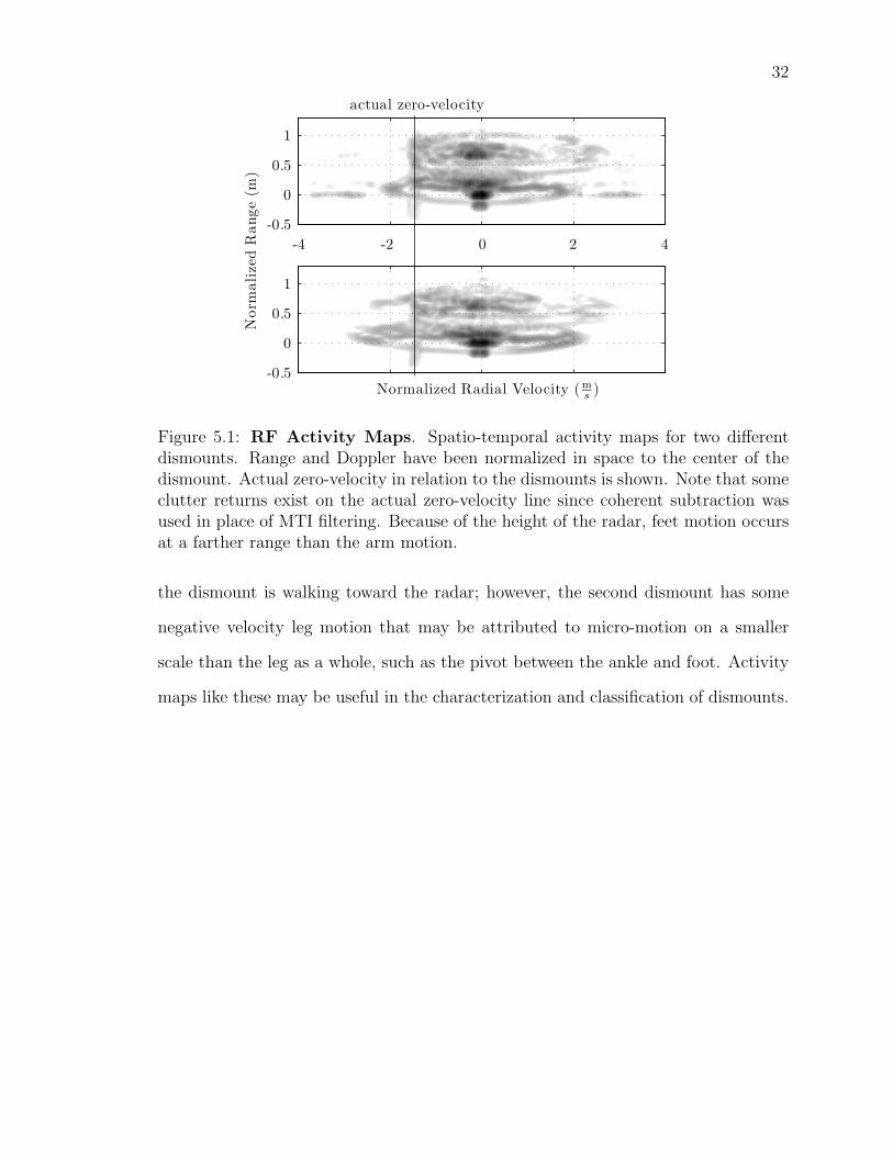
Figure 5.1 shows activity maps of two different dismounts undergoing a standard
walking motion toward the radar. The activity maps were formed by integrating over
a single gait cycle with window lengths of 256 pulses and an overlap of 200 pulses.
The motion of the arms and legs and their radial velocities can clearly be seen. The
second dismount appears to walk with higher velocity arm and leg motions relative
to the torso than the first dismount. Note that the arms swing past actual zero-
velocity, indicating they move away from the radar on their back-swing. Generally,
the feet come in contact with the ground and do not move away from the radar when
32
-4 -2 0 2 4
-0.5
0
0.5
1
Normalized Radial Velocity (ms )
Nor
mal
ized
Ran
ge(m
)
-0.5
0
0.5
1
actual zero-velocity
Figure 5.1: RF Activity Maps. Spatio-temporal activity maps for two differentdismounts. Range and Doppler have been normalized in space to the center of thedismount. Actual zero-velocity in relation to the dismounts is shown. Note that someclutter returns exist on the actual zero-velocity line since coherent subtraction wasused in place of MTI filtering. Because of the height of the radar, feet motion occursat a farther range than the arm motion.
the dismount is walking toward the radar; however, the second dismount has some
negative velocity leg motion that may be attributed to micro-motion on a smaller
scale than the leg as a whole, such as the pivot between the ankle and foot. Activity
maps like these may be useful in the characterization and classification of dismounts.
CHAPTER 6
THREE-DIMENSIONALRECONSTRUCTION
Here, a three-dimensional map is created using the fusion of RF and EO data.
Tomographic algorithms exist in RF and EO domains; however, they each require a
large sweep angle of measurements. By combining the output from the two sensors,
a 3-D map of a walking dismount is formed; however, the micro-motion of the dis-
mount will cause smearing in certain areas of the map. EO tomosynthesis and RF
back-projection are similar algorithms for each of their sensor domains. Each uses
measurments from multiple look angles to create a three-dimensional estimate of the
object of interest.
6.1 RF Back-projection
The ideal image formation process for ISAR imaging involves matched filtering of
the phase history data. A volume in Cartesian space is chosen over which to image.
Continue to let x(τk), y(τk), and z(τk) represent the estimated dismount track in world
coordinates(origin at EO camera center). Let x, y, and z represent the coordinates
with the origin at the center of the 3-D image volume. Assume the coordinate axes of
the image volume are oriented in the same way as the tracking(world) axes such that
conversion between the two coordinate systems is purely translational. The origin of
the image volume is maintained as the center of the dismount returns, so it varies with
respect to slow-time. At a point (x, y, z) in the volume, the matched filter response
33
34
is
P (x, y, z) =1
NfNτ
Nf−1∑i=0
Nτ−1∑k=0
S(fi, τk)ej4πfi
Rxyz(τk)
c (6.1)
where Rxyz(τk) is the range to the imaging point, (x, y, z) at pulse τk. The motion
of the dismount must be compensated for when determining the range to the image
center. The range from the radar to the image center is simply the tracked range of
the dismount given by
R000(τk) =√x(τk)2 + y(τk)2 + z(τk)2 (6.2)
Adjusting (6.2) with the imaging point in the image coordinates gives the range from
the radar to the image point, (x, y, z),
Rxyz(τk) =
√(x+ x(τk))
2 + (y + y(τk))2 + (z + z(τk))
2 (6.3)
Substituting (2.9) into (6.1) and substituting the time delay Txyx = 2Rxyz/c , the
matched filter output is given by
P (x, y, z) =1
NfNτ
Nf−1∑i=0
Nτ−1∑k=0
S(fi, τk)ej2π
„f0+ iB
Nf
«Txyz(τk)
=1
NfNτ
Nτ−1∑k=0
ej2πf0Txyz(τk)
Nf−1∑i=0
S(fi, τk)ej2π iB
NfTxyz(τk)
=1
Nτ
Nτ−1∑k=0
ej2πf0Txyz(τk)U(Txyz(τk)
)(6.4)
where
U(Txyz(τk)
)=
1
Nf
Nf−1∑i=0
S(fi, τk) exp
[j2π
iB
Nf
Txyz(τk)
](6.5)
35
To allow for digital processing, the time delay, Txyz(τk), can be sampled into discrete
values according to
Txyz(τk) =n
B
Nf
NR
(6.6)
where NR is the number of samples in range. Then, U becomes a function of n and
is given by
U(n, τk) =1
Nf
Nf−1∑i=0
S(fi, τk) exp
[j2π
in
NR
], (6.7)
which is the IDFT of the phase history data in the fast-time dimension. The back-
projection algorithm can therefore be performed by (6.4) using the IFFT of the phase
history in fast-time multiplied by the focusing phase, exp [j2πf0Txyz(τk)].
The image P (x, y, z) can be computed at any point in 3-D space; however, a
volume surrounding the dismount is sampled with discrete coordinates, xi, yj, zl.
U(n, τk) provides data sampled along the range dimension; however, P (xi, yj, zl) is
sampled in Cartesian coordinates. Linear interpolation is used to obtain the sam-
ples for U(Txyz(τk)
)from U(n, τk). Because of the use of simple linear interpolation,
range must be oversampled to minimize errors introduced by interpolation and to
maintain phase coherence. In this case, range is oversampled by a factor of 64, giving
NR = 64Nf . Oversampling of U(n) is implemented as zero-padding when performing
the FFT of the phase history data.
6.2 EO Tomosynthesis
Tomosynthesis[31] is analogous to RF back-projection in the EO domain. To-
mosynthesis differs from traditional computed tomography (CT) in a few ways [32].
CT methods usually reconstruct a volume with a large number of projections, where
36
−10
1−1
0
1−1.5
−1
−0.5
0
0.5
1
1.5
yx
z
Figure 6.1: RF Back-projection Results. Radar returns for 1024 pulses are back-projected into 3-D space. Since the dismount sweeps through a small angular range,azimuth resolution is not noticably improved. Results are shown on a dB scale withdarker areas representing stronger returns.
tomosynthesis uses a relatively small number of projections. CT methods also use
a wide range of aspect angles(sometimes full 360◦), while tomosynthesis uses projec-
tions over a small range of aspect angles. For these reasons, CT is well suited for
cooperative subjects and controlled sensor configuration applications, such as medical
imaging, while tomosynthesis is well suited for non-cooperative surveillence applica-
tions where there is insufficient information for CT methods.
Tomosynthesis amounts to back-projecting the image point, γ, to the line, γ(λ)
in 3-space. Back-projection is performed for each pixel in a frame, giving a set of
rays that represent possible locations for the 3-D point that was projected into each
image point. EO back-projection is theoretically defined by
γ(λ) = P+γ + λc (6.8)
37
where P+ is the pseudo-inverse of the camera matrix, P. P+γ converts the image
point, γ, from image coordinates to the 3-D world coordinate system while λc forms
the line between c and γ as λ varies.
Tomosynthesis involves a camera moving around a static object and capturing
views from different aspect angles. In this case, inverse tomosynthesis is used, where
the camera is static and the image volume is moving through the scene. Similar to
RF back-projection imaging, the 3-D image coordinate center, (x, y, z) = (0, 0, 0),
is held at the center of the dismount over time. Therefore, the camera coordinate
system remains static, but the 3-D image coordinate system moves along with the
dismount. The movement of the 3-D image coordinate system is purely translational
so as to preserve the back-projection angles. The 3-D image coordinate axis maintains
the same orientation as the world coordinate system in the RF case. The camera
orientation or position never changes, but as the dismount moves through the frame,
the azimuth angles of the rays formed by the back-projection of the pixels on the
dismount change. Since the camera is static and the dismount is moving along the
ground plane, it is assumed that the projected rays are changing only in azimuth
angle as the dismount moves through the scene. This assumption simplifies the back-
projection process.
Equation (2.7) shows that the azimuth and elevation angles of back-projected rays
can be determined with knowledge of the camera field of view. For each EO frame,
the dismount mask, Gk(u, v), given by (3.10), is back-projected to form a set of rays
in 3-D space. These rays are completely defined by their azimuth (φ) and elevation
(θ) angles and the camera center, through which each ray passes. The camera center
occurs at the origin of the world coordinate system, and the angles are determined
by equation (2.7). The dismount track is used to locate the center of the 3-D image
38
volume to be sampled. Let w represent the 3-D image origin in world space given by
w =
x(k)
y(k)
0
(6.9)
Within the 3-D image volume, the back-projected rays are sampled on the same
discrete Cartisian grid used in RF back-projection, (xi, yj, zl). Each of the rays is
first sampled along the ray at the grid values for y. The sample locations are given
by.
x =(yk + y) arctan [φ(u)]− xk (6.10a)
z =√
(xk + y)2 + (yk + y)2 arctan [θ(v)] (6.10b)
This gives a set of (x, y, z) samples in the 3-D image volume. Each of the samples
corresponds to a binary value that indicates whether or not the ray on which the
sample lies intersected the dismount mask. The sampled rays are interpolated onto
the 3-D image grid using linear interpolation.
Back-projection and interpolation is performed for a sequence of frames, over
which the aspect angle changes, providing different views of the dismount. The 3-D
maps obtained from each frame are on the same coordinate system in relation to
the dismount, so they can simply be integrated. The integration has the effect of
enforcing voxels that lie on the dismount. Let T (xi, yj, zl) represent the sampled
tomosynthesis output given by
T (xi, yj, zl) =∑k
Tk(xi, yj, zl) (6.11)
where Tk is the interpolated back-projection for a single frame.
As in RF back-projection, dismount micro-motion causes blurring in certain areas
39
−10
1−1
0
1−1.5
−1
−0.5
0
0.5
1
1.5
yx
z
Figure 6.2: EO Tomosynthesis Results. Five EO frames containing the samedismount pose are back-projected into 3-D space. Note that some range resolution isachieved. This can be seen as the right and left legs appear to be separated in range.Results are shown on an intensity scale.
since the arms and legs are not integrated into the same location from frame to frame.
By using only EO frames from a single dismount pose, this can be minimized at the
expense of some cross-range resolution. Figure 6.2 shows the tomosynthesis output
using one frame per gait cycle. It is clear that the dismount only sweeps through
enough look angles to remove a fraction of the range ambiguity.
6.3 RF and EO Fusion
The RF and EO 3-D images are fused to form a single 3-D map of the dismount.
A common coordinate system was used in the formation of the RF and EO images,
so the images are already registered in 3-D space. Voxels on the dismount are those
in the intersection of the 3-D maps obtained from the RF and EO imaging. The RF
intensity and EO images are normalized to values from 0 to 1. The final 3-D image is
40
−10
1−1
0
1−1.5
−1
−0.5
0
0.5
1
1.5
yx
z
Figure 6.3: Fused 3-D image. EO and RF back-projected points are fused toform a single 3-D image. The image clearly shows the shape of the dismount andthe extension of the carried object. Results are shown in dB with higher valuescorresponding to darker points.
formed by the voxel-wise multiplication of the normalized RF and EO images. Much
of the ambiguity that exists in the RF and EO images alone is removed in the fused
image.
CHAPTER 7
CONCLUSION
The simultaneous use of RF and EO sensors for dismount characterization and
imaging provides some advantages over the use of each sensor individually. By ex-
ploiting the range information from an RF sensor and the azimuth and elevation
information from an EO sensor, the ambiguities of each of the sensors are diminished.
RF and EO processing techniques were presented as well as a fused tracking algorithm.
3-D images of dismounts were formed using the fusion of tomographic techniques in
the RF and EO domains. Imaging dismounts presents a number of problems because
of their articulated motion. Standard tomographic techniques perform relatively well,
but there is still a need to better compensate for dismount micro-motion when imag-
ing. Future research in this area will involve refining the 3-D imaging techniques to
better handle the human micro-motion and form more accurate images for each time
instant. An accurate 3-D image of a dismount will provide information on dismount
structure and motion.
41
REFERENCES
[1] C. Barclay, J. Cutting, and L. Kozlowski, “Temporal and spatial factors in gaitperception that influence gender recognition.” Percept Psychophys, vol. 1978, pp.145–52, 2002.
[2] J. Cutting and L. Kozlowski, “Recognition of friends by their walk,” Bulletin ofthe Psychonomic Society, vol. 9, pp. 353–356, 1977.
[3] N. Troje, C. Westhoff, and M. Lavrov, “Person identification from biologicalmotion: Effects of structural and kinematic cues,” Perception & Psychophysics,vol. 67, no. 4, pp. 667–675, 2005.
[4] N. V. Boulgouris, D. Hatzinakos, and K. N. Plataniotis, “Gait recognition: achallenging signal processing technology for biometric identification,” IEEE Sig-nal Processing Magazine, vol. 22, no. 6, pp. 78–90, Nov. 2005.
[5] V. C. Chen, “Analysis of radar micro-doppler with time-frequency transform,”in Statistical Signal and Array Processing, 2000. Proceedings of the Tenth IEEEWorkshop on, Pocono Manor, PA, Aug. 2000, pp. 463–466.
[6] V. C. Chen, R. Lipps, and M. Bottoms, “Advanced synthetic aperture radarimaging and feature analysis,” in Radar Conference, 2003. Proceedings of theInternational, Sep. 2003, pp. 22–29.
[7] V. C. Chen, “Spatial and temporal independent component analysis of micro-doppler features,” in Radar Conference, 2005 IEEE International, May 2005,pp. 348–353.
[8] T. Thayaparan, S. Abrol, E. Riseborough, L. Stankovic, D. Lamothe, andG. Duff, “Analysis of radar micro-doppler signatures from experimental heli-copter and human data,” Radar, Sonar & Navigation, IET, vol. 1, no. 4, pp.289–299, Aug. 2007.
[9] J. E. Gray and S. R. Addison, “Effect of nonuniform target motion on radarbackscattered waveforms,” in Radar, Sonar and Navigation, IEE Proceedings -,vol. 150, Aug. 2003, pp. 262–70.
[10] V. C. Chen, F. Li, S. S. Ho, and H. Wechsler, “Micro-doppler effect in radar:phenomenon, model, and simulation study,” IEEE Transactions on Aerospaceand Electronic Systems, vol. 42, no. 1, pp. 2–21, Jan. 2006.
42
43
[11] P. van Dorp and F. C. A. Groen, “Human walking estimation with radar,” Radar,Sonar and Navigation, IEE Proceedings -, vol. 150, no. 5, pp. 356–365, Oct. 2003.
[12] M. Otero, “Application of a continuous wave radar for human gait recognition,”Proc. SPIE, vol. 5809, pp. 538–548, 2005.
[13] J. Li and H. Ling, “Application of adaptive chirplet representation for ISARfeature extraction from targets with rotating parts,” in Radar, Sonar and Navi-gation, IEE Proceedings -, vol. 150, Aug. 2003, pp. 284–91.
[14] S. Stankovic, I. Djurovic, and T. Thayaparan, “Separation of target rigid bodyand micro-doppler effects in ISAR imaging,” IEEE Transactions on Aerospaceand Electronic Systems, vol. 42, no. 4, pp. 1496–1506, Oct. 2006.
[15] R. Hartley and A. Zisserman, Multiple View Geometry in Computer Vision.Cambridge University Press, 2003.
[16] F. J. Harris, “On the use of windows for harmonic analysis with the discretefourier transform,” Proceedings of the IEEE, vol. 66, no. 1, pp. 51–83, Jan. 1978.
[17] B. Gloyer, H. Aghajan, K. Siu, and T. Kailath, “Video-based freeway-monitoringsystem using recursive vehicle tracking,” Proc. SPIE, vol. 2421, pp. 173–180,1995.
[18] B. P. L. Lo and S. A. Velastin, “Automatic congestion detection system forunderground platforms,” in Intelligent Multimedia, Video and Speech Processing,2001. Proceedings of 2001 International Symposium on, Hong Kong, China, 2001,pp. 158–161.
[19] C. Stauffer and W. E. L. Grimson, “Adaptive background mixture models forreal-time tracking,” in Computer Vision and Pattern Recognition, 1999. IEEEComputer Society Conference on., vol. 2, Fort Collins, CO, USA, 1999.
[20] N. M. Oliver, B. Rosario, and A. P. Pentland, “A bayesian computer visionsystem for modeling human interactions,” Transactions on Pattern Analysis andMachine Intelligence, vol. 22, no. 8, pp. 831–843, Aug. 2000.
[21] T. Gevers and A. Smeulders, “Color-based object recognition,” Pattern Recog-nition, vol. 32, no. 3, pp. 453–464, 1999.
[22] M. I. Skolnik, Introduction to radar systems, 1980.
[23] J. Proakis and D. Manolakis, Digital signal processing: principles, algorithms,and applications. Prentice-Hall, Inc. Upper Saddle River, NJ, USA, 1996.
[24] S. Blackman, Multiple-target tracking with radar applications(Book). Dedham,MA, Artech House, Inc., 1986.
44
[25] D. F. Bizup and D. E. Brown, “The over-extended kalman filter - don’t use it!”in Information Fusion, 2003. Proceedings of the Sixth International Conferenceof, vol. 1, 2003, pp. 40–46.
[26] A. F. Bobick and J. W. Davis, “The recognition of human movement usingtemporal templates,” IEEE Transactions on Pattern Analysis and Machine In-telligence, vol. 23, no. 3, pp. 257–267, Mar. 2001.
[27] J. Man and B. Bhanu, “Individual recognition using gait energy image,” IEEETransactions on Pattern Analysis and Machine Intelligence, vol. 28, no. 2, pp.316–322, Feb. 2006.
[28] J. Liu and N. Zheng, “Gait history image: A novel temporal template for gaitrecognition,” in Multimedia and Expo, 2007 IEEE International Conference on,Beijing, China, Jul. 2007, pp. 663–666.
[29] Q. Ma, S. Wang, D. Nie, and J. Qiu, “Recognizing humans based on gait mo-ment image,” in Software Engineering, Artificial Intelligence, Networking, andParallel/Distributed Computing, 2007. SNPD 2007. Eighth ACIS InternationalConference on, vol. 2, Qingdao, China, Jul./Aug. 2007, pp. 606–610.
[30] G. Wang and Z. Bao, “The minimum entropy criterion of range alignment inISAR motioncompensation,” in Radar 97 (Conf. Publ. No. 449), Edinburgh,UK, Oct. 1997, pp. 236–239.
[31] D. G. Grant, “Tomosynthesis: A three-dimensional radiographic imaging tech-nique,” IEEE Transactions on Biomedical Engineering, vol. 19, no. 1, pp. 20–28,Jan. 1972.
[32] T. Persons, P. Hemler, and R. Plemmons, “3d iterative restoration of tomosyn-thetic images.”
[33] J. Lei, “Pattern recognition based on time-frequency distributions of radar micro-doppler dynamics,” in Software Engineering, Artificial Intelligence, Networkingand Parallel/Distributed Computing, 2005 and First ACIS International Work-shop on Self-Assembling Wireless Networks. SNPD/SAWN 2005. Sixth Interna-tional Conference on, May 2005, pp. 14–18.
[34] N. Willis and H. Griffiths, Advances in Bistatic Radar. SciTech Pub, 2007.
[35] N. V. Boulgouris and Z. X. Chi, “Gait recognition using radon transform andlinear discriminant analysis,” IEEE Transactions on Image Processing, vol. 16,no. 3, pp. 731–740, Mar. 2007.