Since the free-vibration response x t ( ) One Degree of ...pirun.ku.ac.th/~fengwtc/Teaching/208322...

208322 Mechanical Vibrations Lesson 6

1 Copyright 2007 by Withit Chatlatanagulchai

One Degree of Freedom, Harmonically Excited Vibrations

1 Forced Harmonic Vibration A mechanical system is said to undergo forced vibration whenever external energy is supplied to the system during vibration. External energy can be from either an applied force or an imposed displacement excitation. The applied force or displacement excitation may be harmonic, nonharmonic but periodic, nonperiodic, or random. Harmonic excitations are of the forms, for example,

( ) ( )

( ) ( )( ) ( )

0

0

0

,

cos ,

sin ,

i tF t F e

F t F t

F t F t

ω

ω

ω

+Φ=

= +Φ

= +Φ

where 0F is the amplitude, ω is the frequency, and Φ is the phase angle

usually taken to be zero. Under a harmonic excitation, the response of the system will also be harmonic with the same frequency as the excitation frequency. If the frequency of the harmonic excitation is close to the system natural frequency, the beating phenomenon will happen. This condition, known as resonance, is to be avoided to prevent failure of the system. Consider a system in Figure 1. The equation of motion is

( ).mx cx kx F t+ + =��

Its general solution is

( ) ( ) ( ) ,h px t x t x t= +

where ( )hx t is the homogeneous solution (the solution when ( ) 0F t = as

was studied in the free vibration) and ( )px t is the particular solution.

Since the free-vibration response ( )hx t dies out with time under each of

the three conditions of damping (underdamping, critical damping, and overdamping), the general solution eventually reduces to the particular

solution ( ) ,px t which represents the steady-state vibration. Figure 2

shows homogeneous, particular, and general solutions for the underdamped case.

Figure 1: A spring-mass-damper system.

Figure 2: Homogeneous, particular, and

general solutions for the underdamped case.



1.1 Undamped System under 0 cosF tω

Consider the system in Figure 1 but without damper. If a force

( ) 0 cosF t F tω= acts on the mass m, the equation of motion is given by

0 cos .mx kx F tω+ =�� (1)

The solution is

( ) ( ) ( ) ,h px t x t x t= +

where

( )( )

1 2cos sin ,

cos .

h n n

p

x t C t C t

x t X t

ω ω

ω

= +

= (2)

Applying initial conditions ( ) 00x x= and ( ) 00 ,x x=� � and by substituting

(2) into (1), the three unknowns 1 2, ,C C and X can be solved, then the

solution becomes

( ) 0 0 00 2 2

cos sin cos .n n

n

F x Fx t x t t t

k m k mω ω ω

ω ω ω = − + + − −

�

Letting 0 /st

F kδ = denote the static deflection of the mass under a

force 0 ,F we have

2

1.

1st

n

X

δ ωω

=

−

(3)

The quantity /st

X δ represents the ratio of the dynamic to the static

amplitude of motion and is called amplitude ratio.

The total response (2) can also be written in three cases as follows:

1) For / 1,n

ω ω < we have

( ) ( ) 2cos cos .

1

stn

n

x t A t tδ

ω ωωω

= −Φ +

−

2) For / 1,n

ω ω > we have

( ) ( ) 2cos cos .

1

stn

n

x t A t tδ

ω ωωω

= −Φ −

−

3) For ,n

ω ω≈ we have a beating phenomenon. Letting 0 0 0,x x= =� we

have

( ) ( ) ( )

( )

0

2 2

0

2 2

/cos cos

/2sin sin .

2 2

n

n

n n

n

F mx t t t

F mt t

ω ωω ω

ω ω ω ωω ω

= −−

+ − = ⋅ −

(4)

Let the forcing frequency ω be slightly less than the natural frequency:

2 .n

ω ω ε− = (5)

Then n

ω ω≈ we have

2 .n

ω ω ω+ ≈ (6)

Using (5) and (6), (4) becomes



( ) 0 /sin sin .

2

F mx t t tε ω

εω =

Define period of beating to be ( )2 / 2 2 / .b n

τ π ε π ω ω= = − Define

frequency of beating to be 2 .b n

ω ε ω ω= = −

The plots of the total responses of all three cases are given in Figure 3.

Figure 3: Plots of total responses of the three

cases.



☻ Example 1: [1] A reciprocating pump with mass 68 kg is mounted as shown below at the middle of a steel plate of thickness 1 cm, width 50 cm, and length 250 cm. During operation, the plate is subjected to a harmonic

force ( ) 220 cos62.832F t t= N. Find the amplitude of vibration of the

plate.

Solution The plate can be modeled as a fixed-fixed beam with equivalent spring constant

( ) ( )( )

( )

3

39 2 2

32

192

1192 200 10 50 10 10

12

250 10

102400.82 / .

EIk

l

N m

− −

−

=

× × =

×

=

From (3), we have

0

2

2

/

1

220 /102400.82

62.8321

102400.82 / 68

0.001325 .

n

F kX

m

ωω

=

−

=

−

= −

The negative sign indicates that the response ( )x t is out of phase

with the excitation ( ).F t



1.2 Damped System under 0 cosF tω

For the damped system, the equation of motion becomes

0 cos .mx cx kx F tω+ + =�� (7)

Assume the particular solution in the form

( ) ( )cos ,p

x t X tω= −Φ

where X and Φ are unknown constants to be determined. Substituting

into (7) and equating the coefficients of cos tω and sin tω on both sides,

we obtain

( )0

1/ 22

2 2 2

FX

k m cω ω= − +

and

1

2tan .

c

k m

ωω

− Φ = −

Figure 4 shows plots of forcing function and particular solution.

Recall that /n

k mω = = undamped natural frequency,

/ / 2 ,c n

c c c mζ ω= = 0 /st

F kδ = = deflection under the static force 0 ,F

and /n

r ω ω= = frequency ratio. The amplitude ratio and the phase angle

is given by

1/ 2 2 2 22

2 2

1 1

(1 ) (2 )

1 2

st

n n

X

r rδ ζω ω

ζω ω

= =− + − +

(8)

Figure 4: Representation of forcing function

and response. and

1 1

2 2

22

tan tan1

1

n

n

r

r

ωζω ζ

φωω

− −

= = − −

The plots of amplitude ratio and phase angle versus frequency ratio are given in Figure 5 and Figure 6 respectively. The total response is given by

( ) ( ) ( ).h px t x t x t= +

For an underdamped system, we have

0 0( ) cos( ) cos( )nt

dx t X e t X t

ζω ω φ ω φ−= − + −



where 21 .

d nω ζ ω= − 0X and 0Φ are unknown constants to be

determined from initial conditions. For the initial conditions ( ) 00x x= and

( ) 00 ,x x=� � we have two equations to solve for two unknowns

0 0 0

0 0 0 0 0 0

cos cos ,

cos sin sin .n d

x X X

x X X X

φ φ

ζω φ ω φ ω φ

= +

= − + +� (9)

Figure 5: Variation of /st

X δ with .r

Figure 6: Variation of Φ with .r



☻ Example 2: [1] Find the total response of a single degree of freedom

system with 010 , 20 / , 4000 / , 0,m kg c N s m k N m x= = − = =� and

0 0.01x = under an external force ( ) 0 cosF t F tω= with 0 100F N= and

10 / .rad sω =

Solution From the data, we have

( )( )

( ) ( )

0

22

/ 4000 /10 20 / ,

/ 100 / 4000 0.025 ,

/ / 2 20 / 2 4000 10 0.05,

1 1 0.05 20 19.97 / ,

/ 10 / 20 0.5.

n

st

c

d n

n

k m rad s

F k m

c c c km

rad s

r

ω

δ

ζ

ω ζ ω

ω ω

= = =

= = =

= = = =

= − = − =

= = =

1/ 22 2 2 2 2 2

0.0250.03326m

(1 ) (2 ) (1 0.05 ) (2 0.5 0.5)

stXr r

δ

ζ= = =

− + − + ⋅ ⋅

1 1

2 2

2 2 0.05 0.5tan tan 3.814075

1 1 0.5

r

r

ζφ − − ⋅ ⋅ = = = ° − −

Substituting the data above into (9), we get

0 0.0233X = and 0 5.587 .Φ = �

For small values of damping, we can take

max

1

2n

st st

X XQ

ω ωδ δ ζ

=

≈ = =

. (10)

The difference between the frequencies associated with the half power

( / 2Q ) points 1R and 2R is called bandwidth of the system.

/ stX δ

/ nω ω2R1.01R

1

2Q

ζ=

2

Q

Bandwidth

Figure 7: Harmonic response curve showing half power points and bandwidth.

To find 1R and 2R , we set / / 2st

X Qδ = in (8) to obtain

4 2 2 2(2 4 ) (1 8 ) 0r r ζ ζ− − + − =

whose solutions are



2 2

2 2 2 21 21 1 2 2

1 2 , 1 2n n

r R r Rω ω

ζ ζω ω

= = ≈ − = = ≈ +

.

Using the relation 2 1 2n

ω ω ω+ = and

2 2 2 2 2 2

2 1 2 1 2 1 2 1( )( ) ( ) 4n n

R Rω ω ω ω ω ω ω ζω− = + − = − ≈ , we have that

the bandwidth is given by

2 1 2 .n

ω ω ω ζω∆ = − ≈

Combining the bandwidth equation with (10), we obtain

2 1

1

2

nQω

ζ ω ω≈ ≈

−.

It can be seen that Q can be used for estimating the equivalent viscous

damping and the natural frequency in mechanical systems.

1.3 Damped System under 0

i tF e

ω

Let the harmonic forcing function be represented in complex form

as ( ) 0 .i t

F t F eω= The equation of motion becomes

0 .i t

mx cx kx F eω+ + =�� (11)

Assume the particular solution

( ) .i t

px t Xe

ω=

Substituting into (11), we have

0

2

2

0 2 2 2 2 2 2 2 2

0

1/ 22 2 2 2

( )

( ) ( )

,( )

i

FX

k m ic

k m cF i

k m c k m c

Fe

k m c

φ

ω ω

ω ωω ω ω ω

ω ω−

=− +

−= − − + − +

= − +

where

1

2tan .

c

k m

ωφ

ω− = −

Thus, the particular solution (or steady-state solution) becomes

( )0

1/ 22 2 2

( )( ) ( )

i t

p

Fx t e

k m c

ω φ

ω ω−=

− +

. (12)

The complex frequency response of the system is defined to be

2

0

1( )

/ 1 2

XH i

F k r i rω

ζ≡ =

− +

whose magnitude is given by

( )( ) ( )

1/ 22 220

1.

1 2

kXH i

Fr r

ωζ

= = − +

( )H iω can be used in the experimental determination of the system

parameters ( , ,m c and .)k



If ( ) 0 cos ,F t F tω= the corresponding particular solution is the

real part of (12), which is

0

1/ 22 2 2

( ) cos( ).( ) ( )

p

Fx t t

k m cω φ

ω ω= − − +

If ( ) 0 sin ,F t F tω= the corresponding particular solution is the imaginary

part of (12), which is

0

1/ 22 2 2

( ) sin( ).( ) ( )

p

Fx t t

k m cω φ

ω ω= − − +

(13)

2 Support Motion Sometimes the base or support of a spring-mass-damper system undergoes harmonic motion, as shown in Figure 8.

Figure 8: Base excitation.

The equation of motion is given by

( ) ( ) 0.mx c x y k x y+ − + − =��

Supposing that ( ) sin ,y t Y tω= the equation of motion becomes

sin cos

sin( ),

mx cx kx ky cy kY t c Y t

A t

ω ω ωω α

+ + = + = +

= −

��

where 2 2 1( ) and tan

cA Y k c

k

ωω α − = + = −

. This is similar to

having the forcing function ( ) 0 sinF t F tω= acting on the system and the

same analysis as the previous section can be applied. The particular solution is similar to (13) and is given by

( )

1

2 2

11/ 22 2 2

( ) sin( )

( )sin( )

( ) ( )

sin ,

px t X t

Y k ct

k m c

X t

ω φ α

ωω φ α

ω ω

ω φ

= − −

+= − − − +

= −

,

where 1

1 2tan

c

k m

ωφ

ω− = −

and

3 31 1

2 2 2 2

2tan tan .

( ) ( ) 1 (4 1)

mc r

k k m c r

ω ζφ

ω ω ζ− −

= = − + + −

2.1 Displacement Transmissibility

The ratio of the amplitude of the response ( )px t to that of the

base motion ( )y t , X

Y, is called the displacement transmissibility. The

ratio is given by



1/ 2 1/ 22 2 2

2 2 2 2 2

( ) 1 (2 ).

( ) ( ) (1 ) (2 )

X k c r

Y k m c r r

ω ζω ω ζ

+ += = − + − +

The plots between /X Y and φ versus frequency ratio /n

r ω ω= is given

in Figure 9.

Figure 9: The plots between /X Y and φ

versus frequency ratio /n

r ω ω= .

2.2 Force Transmissibility Let F be the force transmitted to the base or support due to the reactions from the spring and the dashpot. We have

( ) ( )F k x y c x y mx= − + − = −� � ��.

The steady-state solution ( )px t was found to be ( ) ( )sin .

px t X tω φ= −

Therefore,

2 sin( ) sin( )T

F m X t F tω ω φ ω φ= − = − .

TF is called dynamic force amplitude. The ratio /

TF kY is called the force

transmissibility and is given by



1/ 22

2

2 2 2

1 (2 )

(1 ) (2 )

TF r

rkY r r

ζζ

+= − +

.

Figure 10 shows the force transmissibility. The force transmissibility concept is used in the design of vibration isolation systems.

Figure 10: Force transmissibility.

2.3 Relative Motion Let z x y= − denote the motion of the mass relative to the base.

The equation of motion becomes

2 sin .mz cz kz my m Y tω ω+ + = − =��

The steady-state solution is given similar to (13) by

2

111/ 2

2 2 2

sin( )( ) sin( )

( ) ( )

m Y tz t Z t

k m c

ω ω φω φ

ω ω

−= = − − +

,

where 2 2

2 2 2 2 2 2( ) ( ) (1 ) (2 )

m Y rZ Y

k m c r r

ω

ω ω ζ= =

− + − +,

1 1

1 2 2

2tan tan

1

c r

k m r

ω ζφ

ω− − = = − −

.

The ratio /Z Y is shown in Figure 11 and plot of 1φ is in Figure 6.

Figure 11: Relative Motion plot.



☻ Example 3: [1] Consider a simple model of a motor vehicle below. The vehicle has a mass of 1200 kg. The spring constant is 400 kN/m and the damping ratio of 0.5.ζ = If the vehicle speed is 20 km/hr, determine the

displacement amplitude of the vehicle. The road surface varies sinusoidally

with an amplitude of 0.05Y m= and a wavelength of 6 m.

Solution From the given data, we can compute the following quantities:

20 1000 12 2 0.291 / ,

3600 6f rad sω π π

× = = =

1/ 23

400 1018.2574 rad/s,

1200n

k

mω

×= = =

5.817780.318653

18.2574n

rωω

= = = ,

1/ 22

2 2 2

1/ 22

2 2

1 (2 )

(1 ) (2 )

1 (2 0.5 0.318653),

(1 0.318653) (2 0.5 0.318653)

X r

Y r r

ζζ

+=

− +

+ × ×=

− + × ×

1.469237 1.469237(0.05) 0.073462 m.X Y= = =



☻ Example 4: [1] A heavy machine, weighing 3000 N, is supported on a

resilient foundation. The foundation has spring stiffness 40,000 / .k N m=

The machine vibrates with an amplitude of 1 cm when the base of the foundation is subjected to harmonic oscillation at the undamped natural frequency of the system with an amplitude of 0.25 cm. Find (a) the damping constant of the foundation, (b) the dynamic force amplitude on the base, and (c) the amplitude of the displacement of the machine relative to the base. Solution

a) Since ,n

ω ω= we have 1.r = Therefore,

( )( )

1/ 22

2

1 20.014 .

0.0025 2

X

Y

ζ

ζ

+= = =

We then have 0.1291.ζ = The damping constant is given by

2 903.05 / .c

c c km N s mζ ζ= ⋅ = = −

b)

1/ 22

2

1 4400 .

4T

F Yk Nζ

ζ +

= =

c) ( )0.0025

0.009682 2 0.1291

YZ m

ζ= = = .

3 Rotating Unbalance Consider a machine with rotating unbalanced masses in Figure 12.

Figure 12: A machine with rotating

unbalanced masses.



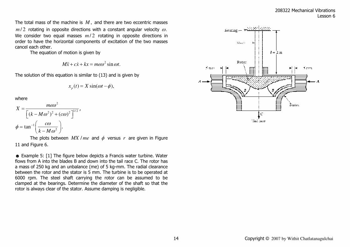
The total mass of the machine is ,M and there are two eccentric masses

/ 2m rotating in opposite directions with a constant angular velocity .ω

We consider two equal masses / 2m rotating in opposite directions in

order to have the horizontal components of excitation of the two masses cancel each other. The equation of motion is given by

2 sin .Mx cx kx me tω ω+ + =��

The solution of this equation is similar to (13) and is given by

( ) sin( ),p

x t X tω φ= −

where 2

1/ 22 2 2( ) ( )

meX

k M c

ω

ω ω= − +

,

1

2tan

c

k M

ωφ

ω− = −

.

The plots between /MX me and φ versus r are given in Figure

11 and Figure 6. ☻ Example 5: [1] The figure below depicts a Francis water turbine. Water flows from A into the blades B and down into the tail race C. The rotor has a mass of 250 kg and an unbalance (me) of 5 kg-mm. The radial clearance between the rotor and the stator is 5 mm. The turbine is to be operated at 6000 rpm. The steel shaft carrying the rotor can be assumed to be clamped at the bearings. Determine the diameter of the shaft so that the rotor is always clear of the stator. Assume damping is negligible.



Solution Setting 0,c = we have

2

2

2

2

3 2

2

6 2

( )

(1 )

(5.0 10 ) (200 )0.005

(200 )1

0.004

10.04 10 N/m.

meX

k M

me

k r

kk

k

ωω

ω

ππ

π

−

=−

=−

× ×=

−

= ×

Since for the steel beam,

4

3 3

3 3,

64

EI E dk

l l

π = =

we have

3 4 2 34 4 4

11

64 (64)(10.04 10 )(2 )2.6005 10 m

3 3 (2.07 10 )

kld

E

ππ π

−×= = = ×

× and

0.1270 m 127 mm.d = =

Lesson 6 Homework Problems 3.19, 3.20, 3.30, 3.39, 3.47, 3.52. Homework problems are from the required textbook (Mechanical Vibrations, by Singiresu S. Rao, Prentice Hall, 2004)

References [1] Mechanical Vibrations, by Singiresu S. Rao, Prentice Hall, 2004

Date post:	17-Mar-2018
Category:	Documents
Upload:	ngodang
View:	220 times
Download:	3 times

Since the free-vibration response x t ( ) One Degree of ...pirun.ku.ac.th/~fengwtc/Teaching/208322...

Documents