Single-Model Case Study: AQ Modeling for PM2.5 NAAQS Regulatory Impact Analysis

James T. Kelly Office of Air Quality Planning & Standards US Environmental Protection Agency

1

Outline

I. Background on air quality models II. Single-model case study: PM2.5 NAAQS RIA III. Key considerations in single-model air quality projections IV. Considerations in potential use of multiple models V. Final thoughts

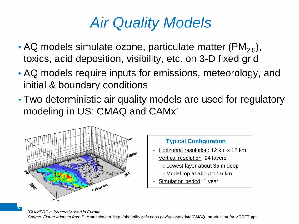
Air Quality Models • AQ models simulate ozone, particulate matter (PM2.5), toxics, acid deposition, visibility, etc. on 3-D fixed grid

• AQ models require inputs for emissions, meteorology, and initial & boundary conditions

• Two deterministic air quality models are used for regulatory modeling in US: CMAQ and CAMx*

*CHIMERE is frequently used in Europe Source: Figure adapted from S. Arunachalam, http://airquality.gsfc.nasa.gov/uploads/data/CMAQ-Introduction-for-ARSET.ppt

2

• Horizontal resolution: 12 km x 12 km • Vertical resolution: 24 layers

oLowest layer about 35 m deep oModel top at about 17.6 km

• Simulation period: 1 year

Typical Configuration

Case Study Overview PM2.5 NAAQS Regulatory Impact Analysis

3

• In December 2012, US EPA strengthened the annual PM2.5 National Ambient Air Quality Standards from 15 µg/m3 to 12 µg/m3

• US EPA was required to estimate the costs and benefits of the rule as part of a Regulatory Impact Analysis (RIA) – AQ modeling provided key inputs to the cost-benefit calculations

performed in the RIA

• The purpose of the RIA is to provide information rather than to form the basis of AQ management decisions*

– However, similar general approaches are used by states in air quality management decision-making for attaining AQ standards

*NAAQS levels are set based on health effects, not cost considerations

AQ Modeling for the PM2.5 NAAQS RIA

4

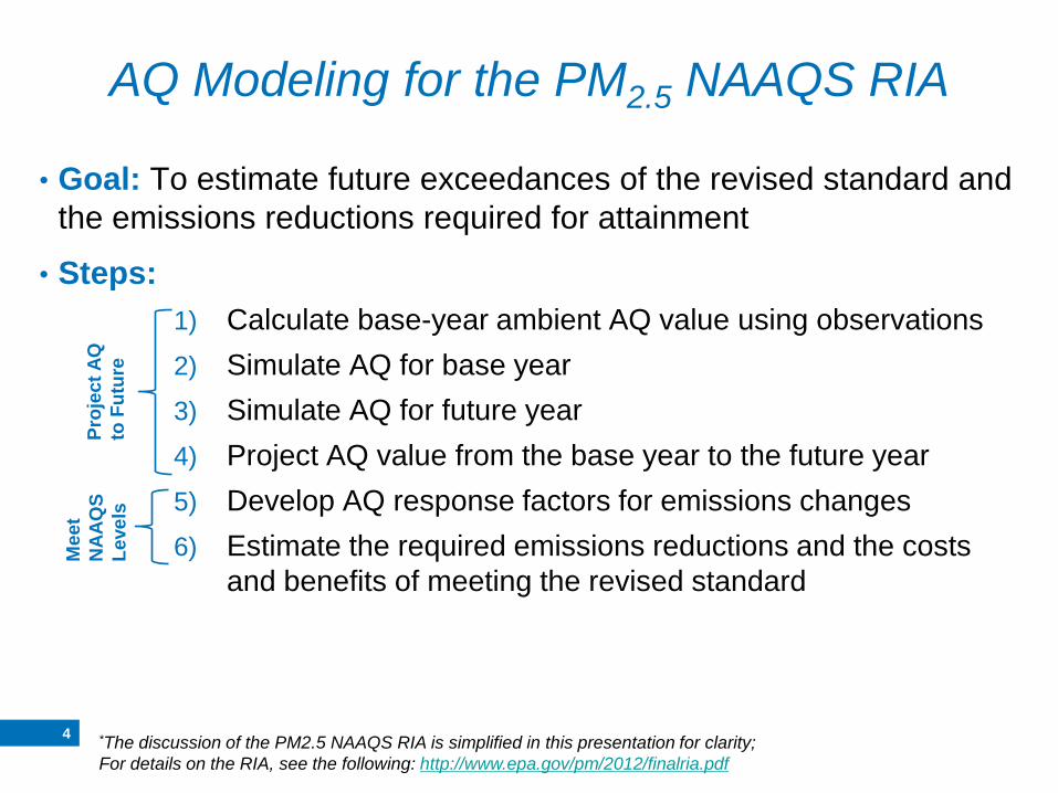
1) Calculate base-year ambient AQ value using observations 2) Simulate AQ for base year 3) Simulate AQ for future year 4) Project AQ value from the base year to the future year 5) Develop AQ response factors for emissions changes 6) Estimate the required emissions reductions and the costs

and benefits of meeting the revised standard

• Goal: To estimate future exceedances of the revised standard and the emissions reductions required for attainment

• Steps:

Proj

ect A

Q

to F

utur

e

Mee

t N

AA

QS

Leve

ls

*The discussion of the PM2.5 NAAQS RIA is simplified in this presentation for clarity; For details on the RIA, see the following: http://www.epa.gov/pm/2012/finalria.pdf

5

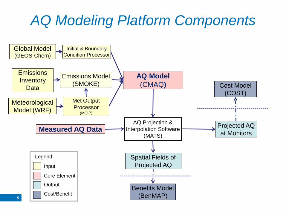
Emissions Inventory

Data

Meteorological Model (WRF)

Emissions Model (SMOKE)

Met Output Processor

(MCIP)

AQ Model (CMAQ)

AQ Projection & Interpolation Software

(MATS) Measured AQ Data Projected AQ

at Monitors

Spatial Fields of Projected AQ

Benefits Model (BenMAP)

Cost Model (COST)

Global Model (GEOS-Chem)

Initial & Boundary Condition Processor

AQ Modeling Platform Components

Input

Output

Core Element

Cost/Benefit

Legend

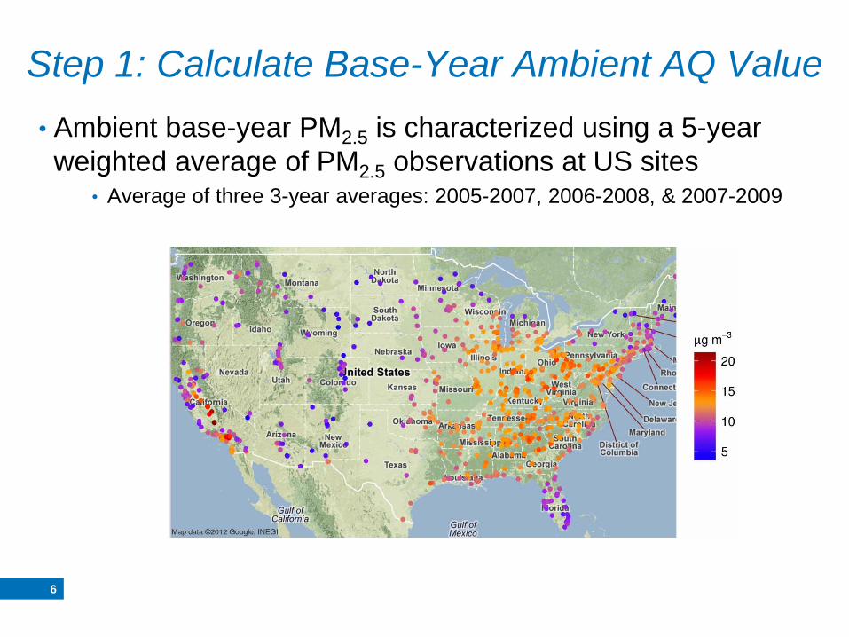
Step 1: Calculate Base-Year Ambient AQ Value

6

• Ambient base-year PM2.5 is characterized using a 5-year weighted average of PM2.5 observations at US sites

• Average of three 3-year averages: 2005-2007, 2006-2008, & 2007-2009

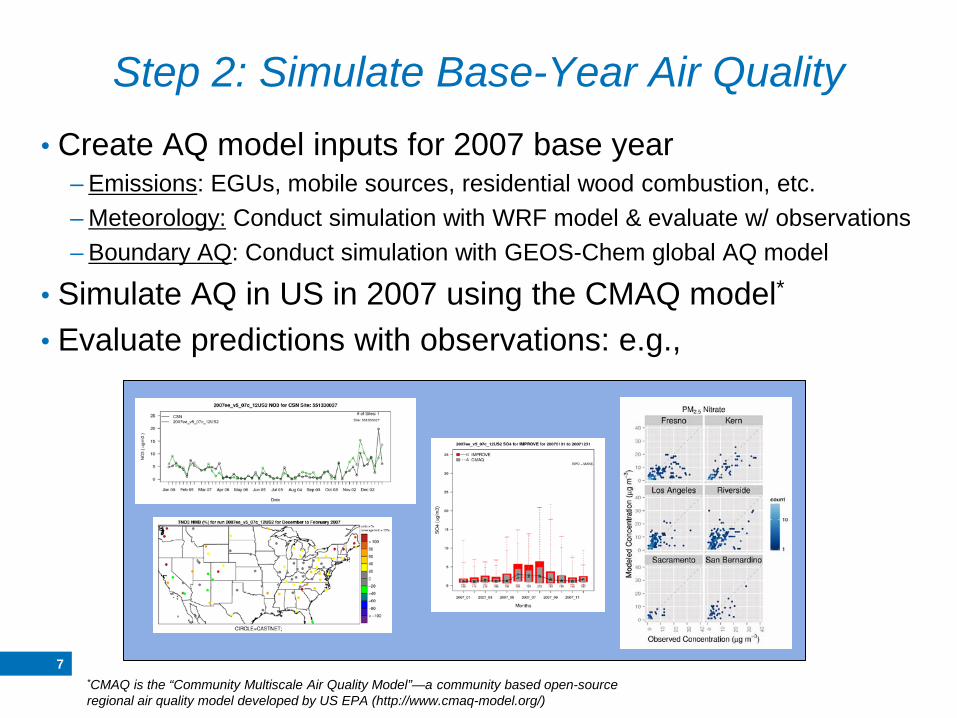
Step 2: Simulate Base-Year Air Quality

7

• Create AQ model inputs for 2007 base year – Emissions: EGUs, mobile sources, residential wood combustion, etc. – Meteorology: Conduct simulation with WRF model & evaluate w/ observations – Boundary AQ: Conduct simulation with GEOS-Chem global AQ model

• Simulate AQ in US in 2007 using the CMAQ model* • Evaluate predictions with observations: e.g.,

*CMAQ is the “Community Multiscale Air Quality Model”—a community based open-source regional air quality model developed by US EPA (http://www.cmaq-model.org/)

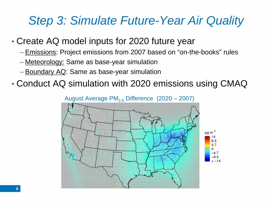
Step 3: Simulate Future-Year Air Quality

8

• Create AQ model inputs for 2020 future year – Emissions: Project emissions from 2007 based on “on-the-books” rules – Meteorology: Same as base-year simulation – Boundary AQ: Same as base-year simulation

• Conduct AQ simulation with 2020 emissions using CMAQ August Average PM2.5 Difference (2020 – 2007)

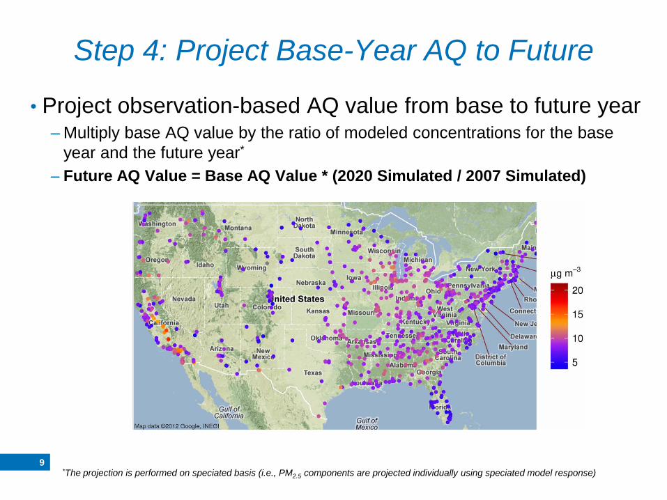
Step 4: Project Base-Year AQ to Future

9

• Project observation-based AQ value from base to future year – Multiply base AQ value by the ratio of modeled concentrations for the base

year and the future year*

– Future AQ Value = Base AQ Value * (2020 Simulated / 2007 Simulated)

*The projection is performed on speciated basis (i.e., PM2.5 components are projected individually using speciated model response)

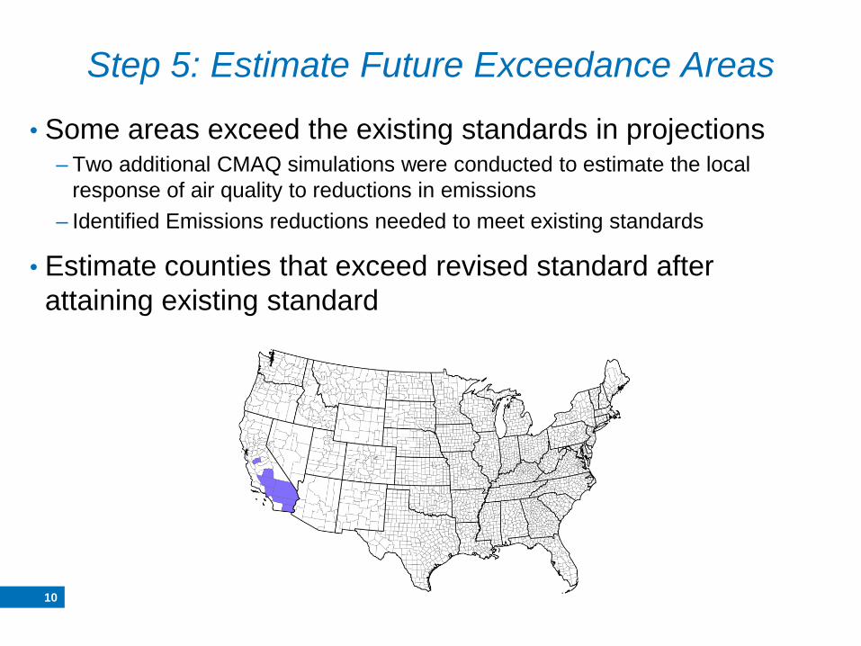
Step 5: Estimate Future Exceedance Areas

10

• Some areas exceed the existing standards in projections – Two additional CMAQ simulations were conducted to estimate the local

response of air quality to reductions in emissions – Identified Emissions reductions needed to meet existing standards

• Estimate counties that exceed revised standard after attaining existing standard

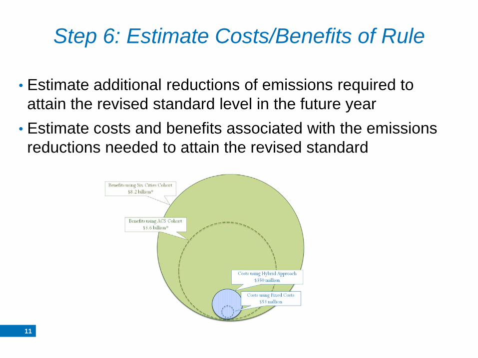
Step 6: Estimate Costs/Benefits of Rule

11

• Estimate additional reductions of emissions required to attain the revised standard level in the future year

• Estimate costs and benefits associated with the emissions reductions needed to attain the revised standard

Considerations in Single-Model Case Study

12

(I) Use of Models in a Relative Sense

13

• Future simulated AQ is not directly used as an estimate of future AQ

• Instead, base-year observed AQ is projected to the future using the ratio of future-year to base-year simulated AQ

• Some evidence suggests that this “relative change” approach can be stable across AQ models – Hogrefe et. al. (2008; JAWMA):

• Up to 20 ppb difference in ozone predictions by different AQ models • Less than a few ppb difference in projected concentrations between different

AQ models – Model bias may cancel out to some degree in the ratio calculation

(II) Projections are Not a “Forecast” of the Future

14

• The base-year AQ value used in projections is based on multi-year averages of observed AQ values – Minimize impacts of inter-annual fluctuations in AQ for stable, data-driven

projection starting point

• AQ simulations are based on a year with meteorology conducive to pollutant formation – Focus AQ management on conditions with pollution episodes

• Same meteorology is used in the base and future year AQ simulations – Isolate the impact of emissions changes from meteorology in projection ratios

• Weight-of-evidence analysis is used to corroborate modeled attainment demonstrations in State Implementation Plans – Considers observed levels, emissions trends, additional modeling, etc.

15

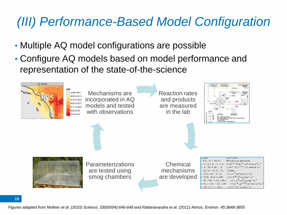
• Multiple AQ model configurations are possible • Configure AQ models based on model performance and

representation of the state-of-the-science

Reaction rates and products are measured

in the lab

Chemical mechanisms

are developed

Parameterizations are tested using smog chambers

Mechanisms are incorporated in AQ models and tested with observations

Figures adapted from Mollner et al. (2010) Science, 330(6004):646-649 and Rattanavaraha et al. (2011) Atmos. Environ. 45:3848-3855

(III) Performance-Based Model Configuration

Considerations in Potential Multiple-Model Studies

16

17

• The number of the air quality “host” models is limited – Two primary models: CMAQ and CAMx – Each has certain unique features that may be critical for a given application

• However, the number of potential model configurations and simulations is vast – Many choices exist for process modules in each AQ model, global model, and

meteorological model; additional choices exist for emissions data – Multiple runs are needed for a given application: e.g., base-year, future-year,

emissions control, and sensitivity runs

• How to select a limited set of cases for multiple modeling? – Current single-model approach selects based on model performance and

state-of-the-science

(I) How to Define the Scope of the Study?

18

• Process representations and their limitations are similar across existing AQ models – Differences between models is likely small compared with the uncertainty

space of interest – Unknown physics and chemistry is unknown to all models – Unknown future emissions changes will be unknown to all models

• Model diversity might be created by configuring AQ models with older modules or parameterizations – Should results based on simulations with low performing configurations be

merged with those of high performing configurations?

(II) Model Diversity

19

• If it were possible to identify the true space of uncertainty, what would the legal implications be? – Does the Clean Air Act allow a probabilistic assessment or would only the

most stringent model result be selected?

(III) Legal Interpretations

(IV) Time Constraints

20

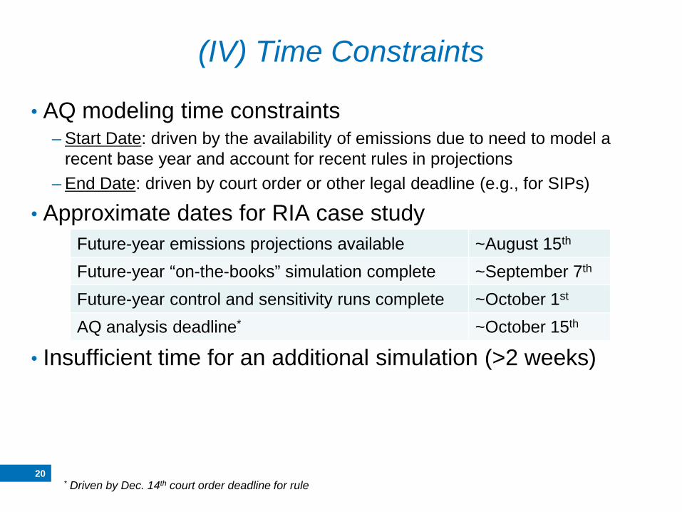
• AQ modeling time constraints – Start Date: driven by the availability of emissions due to need to model a

recent base year and account for recent rules in projections – End Date: driven by court order or other legal deadline (e.g., for SIPs)

• Approximate dates for RIA case study

• Insufficient time for an additional simulation (>2 weeks)

* Driven by Dec. 14th court order deadline for rule

Future-year emissions projections available ~August 15th Future-year “on-the-books” simulation complete ~September 7th Future-year control and sensitivity runs complete ~October 1st AQ analysis deadline* ~October 15th

21

• Select the model configuration based on model performance and representation of the state-of-the-science

• Characterize base-year conditions with observed values – Average base-year data as necessary for a stable starting point

• Project AQ to future using ratios of modeled values rather than directly using future concentration predictions

• Continually evaluate model predictions with data and revise parameterizations and model configuration accordingly

Final Thoughts on Single-Model Approaches