Single molecule fluorescence decay rate statistics in disordered media

Luis FroufeInstituto de Ciencia de Materiales de Madrid, CSIC

Laboratoire Photons et Matière, ESPCI, CNRS

J.J. Sáenz

Universidad autónoma de Madrid

Rémi CarminatiLaboratoire Photons et Matière, ESPCI, CNRS

Molecular levelDifferent modes of operation

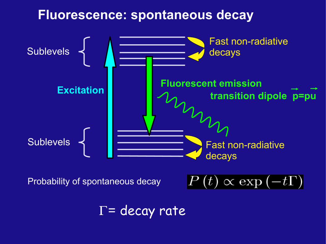
• Intensity signal•Fluorescence lifetime

Applications of fluorescence: Imaging

Whole organ imaging

Combustion

Cell imaging

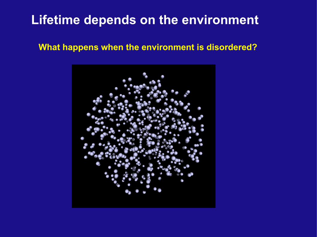
Lifetime depends on the environment

Emission in front of a mirror

Drexhage (1966): fluorescence lifetime of Europium ions depends on source position relative to a silver mirror (l=612 nm)

Silver mirror

Spacer thickness d

Europium ions

Lifetime depends on the environment

Silver nanoparticle, diameter 10 nm

Carminati, Henkel, Greffet, Vigoureux, Opt. Commun. 261, 368 (2006)

Γ

ΓR

ΓNR

Emission in front of a nanoparticle

Z

Lifetime depends on the environment

What happens when the environment is disordered?

Excitation

Fast non-radiative decays

Fast non-radiative decays

Fluorescent emission transition dipole p=pu

Sublevels

Sublevels

Fluorescence: spontaneous decay

Probability of spontaneous decay

= decay rate

Decay rates

Total decay rate

The emitted light can be either radiated out

of the system or absorbed Power (classical)

Decay rate (quantum)

In this talk

Disordered clusters of nanoparticles: statistical properties

•Geometry of the system•Statistics of the emitter•Numerical results•An analytical approach:

oAveraged valuesoFluctuations

Geometry of the system: disordered spherical clusters

R

2R0

Excluded Volume

There is a minimum distance between particles

uncorrelated positions if low filling fraction (f)

a

The emitter

Orientation dynamics SLOWER than

medium dynamics:

taken along one direction

Orientation dynamics FASTER than

medium dynamics:

averaged in all directions

Emission rates in disordered systems: numerical results

f=1%

ε=8+0.01i

Broad distributions.

Strong dependence on absorption level.

Strong dependence on orientation statistics.

Emission rates in disordered systems: numerical results

Non-Radiative contribution increases almost linearly with absorption. Dominating the statistical properties of emission rates.

Radiative contribution does not depend on absorption.

Analytical model•Single scattering•Uncorrelated disorder

Small polarizabilityLow filling fraction

Valid for clusters of nanoparticles

“= N x”

Averaged decay rates

Radiative contribution

•First order term in powers of filling fraction f (single scattering)

•Almost independent on absorption level

ε’=8

Averaged decay rates

Radiative contribution

Explicit separation of terms:

• averaged field

• fluctuations

ε’=8

Averaged radiated field

Averaged decay rates

Radiative contribution

Explicit separation of terms:

• averaged field

• fluctuations

ε’=8

Averaged radiated field Fluctuations far field

Averaged decay rates

Non-Radiative contribution

Averaged decay rates

Non-Radiative contribution

Linear with Im(ε)

Averaged decay rates

Non-Radiative contribution

Linear with Im(ε)

Strong local field effects

Fluctuations of decay rates:

can be explicitly obtained within this model

Relative fluctuations of

(Γ-Γ0)

Relative fluctuations of

(ΓNR)

Fluctuations of decay rates:

can be explicitly obtained within this model

Relative fluctuations of

(Γ-Γ0)

Relative fluctuations of

(ΓNR)

Dominated by scattering in the near field

Fluctuations of decay rates:

can be explicitly obtained within this model

Relative fluctuations of

(Γ-Γ0)

Relative fluctuations of

(ΓNR)

Transition from scattering regime to absorption regime

Fluctuations of decay rates:

can be explicitly obtained within this model

Relative fluctuations of

(Γ-Γ0)

Relative fluctuations of

(ΓNR)

local field effects

Dominated by Non-Radiative coupling

Fixed dipole orientation: statistical distributions

Fixed orientation

Randomly oriented

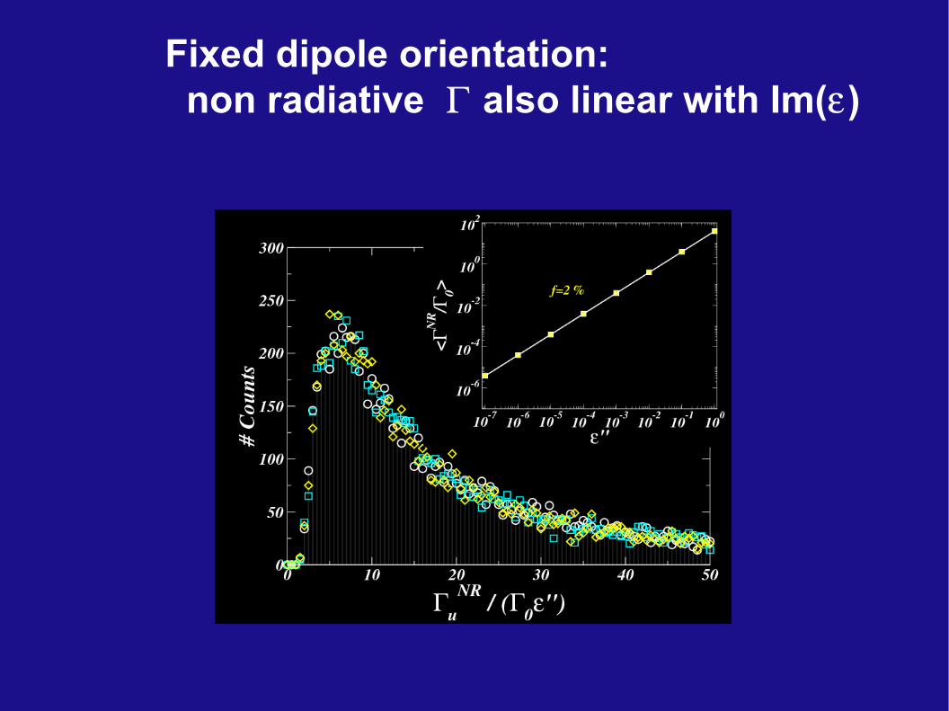
Fixed dipole orientation: non radiative also linear with Im()

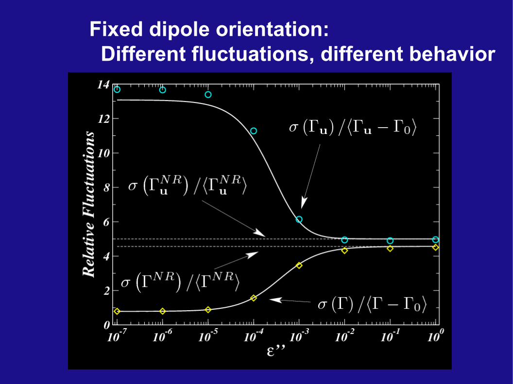
Fixed dipole orientation: Different fluctuations, different behavior

Conclusions

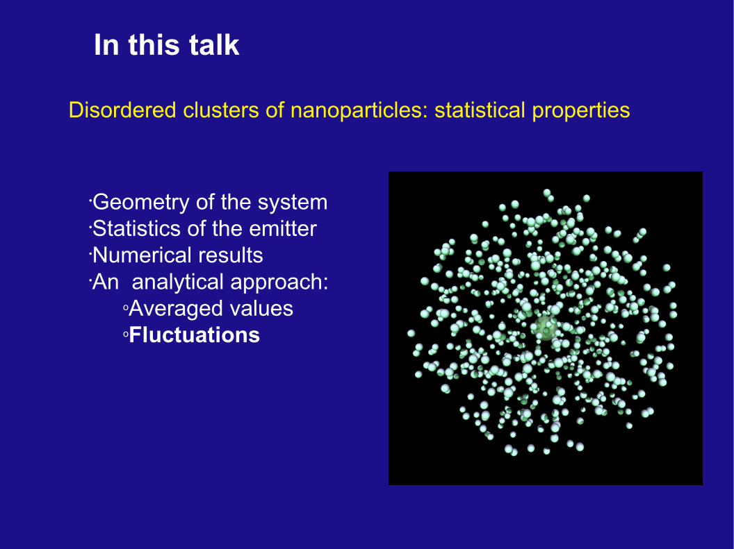
Clusters of small particles

Extensive statistical numerical study.Simple analytical expressions for small clustersRole of near-field scattering.Role Non-Radiative coupling.Strong dependence on the statistics of the orientation of the emitterStrong deppendence on the miscroscopic (subwave-length) environment of the emitter

More Info: L. S. Froufe-Pérez, R. Carminati, and J. J. SáenzPhys. Rev. A 76, 013835 (2007)L. S. Froufe-Pérez and R. CarminatiPhys. Stat. Sol. a, in press (2008)

Additional information

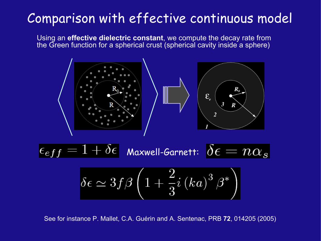
Comparison with effective continuous modelUsing an effective dielectric constant, we compute the decay rate from the Green function for a spherical crust (spherical cavity inside a sphere)

Maxwell-Garnett:

See for instance P. Mallet, C.A. Guérin and A. Sentenac, PRB 72, 014205 (2005)

Comparison with effective continuous model

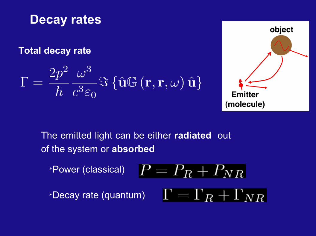
Total decay rate

We obtain the same expression as the one given by the statistical model.

AbsorptionAveraged radiated field Fluctuations of the radiated field

Single Scattering statistical modelInstead of solving the exact problem, we can use a single scattering approach:The field exciting any dipole only comes from the source.

Small polarizability.Low filling fraction.

valid for clusters of nanoparticles

Close to the resonance, the polarizability is large. The single scattering approach fails

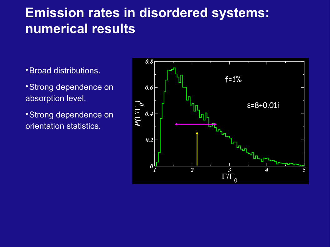
f=1%

Averaged Quantum YieldAveraged Quantum YieldEven in the absorption regime, averaged quantum yield is high enough to obtain a measurable signal

Relative fluctuations of (Γ-Γ0)

Relative fluctuations of (ΓNR)

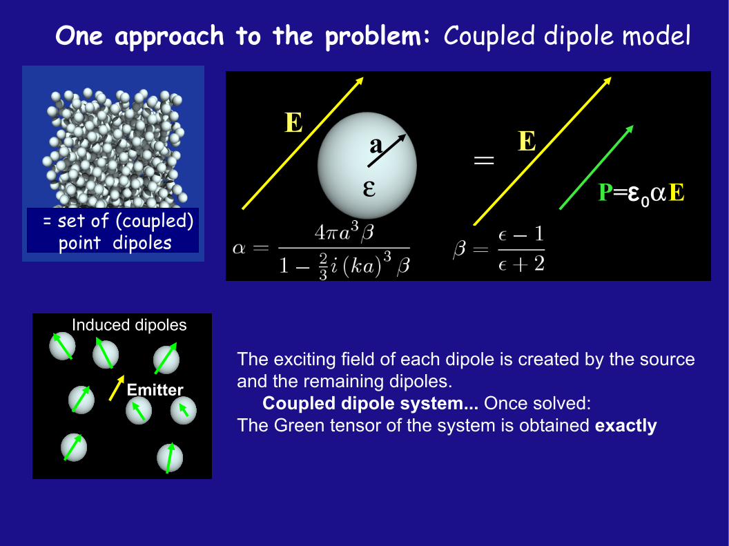
One approach to the problem: Coupled dipole model

= set of (coupled) point dipoles

The exciting field of each dipole is created by the source and the remaining dipoles. Coupled dipole system... Once solved:The Green tensor of the system is obtained exactly

Emitter

Induced dipoles

=E

P=ε0E

a

E