Ruprechts-Karl-Universit ¨ at Heidelberg Naturwissenschaftlich-Mathematische Gesamtfakult ¨ at Inauguraldissertation zur Erlangung der Doktorw¨ urde Singular fibers of Hitchin systems Johannes Horn supervised by Prof. Dr. Anna Wienhard Dr. Daniele Alessandrini First referee Dr. Daniele Alessandrini Date of oral examination: ...
Transcript
Ruprechts-Karl-Universitat Heidelberg
Naturwissenschaftlich-MathematischeGesamtfakultat
Inauguraldissertation zur Erlangung der Doktorwurde
Singular fibers of Hitchin systems
Johannes Horn
supervised by
Prof. Dr. Anna WienhardDr. Daniele Alessandrini
First referee
Dr. Daniele Alessandrini
Date of oral examination:
. . .
iii
Abstract. In the recent years, Hitchin systems and Higgs bundle modulispaces were intensively studied in mathematics and physics. Two major break-throughs were the formulation of Langlands duality of Hitchin systems and theunderstanding of the asymptotics of the hyperkahler metric on Higgs bundle mod-uli space. Both results were considered for the regular locus of the Hitchin systemand both results are conjectured to extend to the singular locus. In this work,we make the first steps towards generalizing these theorems to singular Hitchinfibers.
To that end, we develop spectral data for a certain class of singular fibers ofthe symplectic and odd orthogonal Hitchin system. These spectral data consist ofabelian coordinates taking value in an abelian torsor and non-abelian coordinatesparametrising local deformations of the Higgs bundles at the singularities of thespectral curve. First of all, these semi-abelian spectral data allow us to obtain aglobal description of singular Hitchin fibers. Moreover, we can construct solutionsto the decoupled Hitchin equation on the singular locus of the Hitchin map.These are limits of solutions to the Hitchin equation along rays to the ends ofthe moduli space playing an important role in the analysis of the asymptoticsof the hyperkahler metric. Finally, we can explicitly describe how Langlandsduality extends to this class of singular Hitchin fibers. We discover a dualityon the abelian part of the spectral data, similar to regular case. Instead, thenon-abelian coordinates are symmetric under this Langlands correspondence.
iv
Zusammenfassung. Hitchin-Systeme und Higgs-Bundel-Moduliraume er-fuhren in den letzten Jahren ein wiedererstarktes Interesse von Seiten der Mathe-matik und Physik. Dies fuhrte zu zwei großen Durchbruchen: Zum einen zur For-mulierung der Langlands-Dualitat von Hitchin-Systemen und zum anderen zurAnalyse der Asymptotik der hyperkahlerschen Metrik. Beide Resultate wur-den bisher fur den regularen Lokus der Hitchin-Abbildung bewiesen. Es wirdallerdings vermutet, dass sich beide Resultate auf den singularen Lokus fortsetz-en lassen. Diese Arbeit will die ersten Schritte in diese Richtung gehen, indemgezeigt wird, wie sich Teilresultate auf singulare Hitchin-Fasern erweitern lassenund welche neuen Herausforderungen sich ergeben.
Zu diesem Zweck werden Spektraldaten fur eine bestimmte Klasse singularerFasern des symplektischen und ungerade orthogonalen Hitchin-Systems eingefuhrt.Diese Spektraldaten bestehen aus abelschen Koordinaten mit Werten in einemabelschen Torsor und nichtabelschen Koordinaten, die lokale Transformationendes Higgs-Bundels an den Singularitaten der Spektralkurve beschreiben. Zunachstvermitteln diese halbabelschen Spektraldaten ein globales Verstandnis der Geo-metrie der singularen Hitchin-Fasern. Weiterhin konnen mit ihrer Hilfe Losungzur entkoppelten Hitchin-Gleichung konstruiert werden. Die Losungen dieserGleichung haben beim Verstandnis der Asymptotik der hyperkahlerschen Metrikauf dem regularen Lokus eine wichtige Rolle gespielt. Schlussendlich, kann durchden direkten Vergleich der singularen Fasern eine Fortsetzung der Langlands-Korrespondenz auf den singularen Lokus formuliert werden. In den abelschen Ko-ordinaten wird wie im regularen Fall eine Dualitat beobachtet. Die nichtabelschenKoordinaten hingegen sind symmetrisch unter der Langlands-Korrespondenz.
v
Acknowledgement. Zu allererst will ich meiner geliebten Ehefrau Franziskafur ihre standige Unterstutzung wahrend meines mathematischen Werdegangsdanken. Danke, dass du so manche Einschrankung, die dieser fur unser person-liches Leben mit sich brachte, gerne mitgetragen hast.
The author is in debt to Daniele Alessandrini for his enduring support throughthe preparation of this work, for answering all those questions and for giving methe freedom of developing my own mathematical interests. Furthermore, greatthanks to Anna Wienhard for letting me be part of this great research groupin Heidelberg and for giving me plenty of opportunities to meet mathematiciansall around the world. A special thanks to Beatrice Pozzetti for her stimulatingenthusiasm for mathematics and for having a sympathetic ear for all kinds ofconcerns. Last but not least, the author thanks Xuesen Na, Andy Sanders,Richard Wentworth and Brian Collier for many fruitful discussions.
The author is very grateful for being an active member of the Faculty ofMathematics and Computer Science at University of Heidelberg for the lastfour years. The author acknowledges funding by the Deutsche Forschungsge-meinschaft (DFG, German Research Foundation) – 281869850 (RTG 2229), theKlaus Tschira Foundation, and the U.S. National Science Foundation grants DMS1107452, 1107263, 1107367 ”RNMS: GEometric structures And Representationvarieties” (the GEAR Network).
Contents
Introduction 1Reader’s guide 8
Chapter 1. Preliminaries 91.1. Notation 91.2. Higgs bundle moduli spaces 101.3. Hitchin systems and spectral data 121.4. Abelian varieties 16
Chapter 2. Semi-abelian spectral data for singular fibers of the SL(2,C)-Hitchin system 21
2.1. The SL(2,C)-Hitchin system 212.2. σ-invariant Higgs bundles on the normalised spectral curve 232.3. Hecke transformations 272.4. Moduli of σ-invariant Higgs bundles 312.5. Stratification of singular fibers of the SL(2,C)-Hitchin system 382.6. Singular fibers with locally irreducible spectral curve 392.7. Singular fibers with irreducible spectral curve 502.8. Real points in singular Hitchin fibers 54
Chapter 3. Interlude: Hecke transformations and pushforwards 593.1. Hecke transformations and Hecke modifications 603.2. The pushforward 61
Chapter 4. sl(2)-type fibers of symplectic and orthogonal Hitchin systems 674.1. The Sp(2n,C)-Hitchin system 674.2. sl(2)-type fibers of symplectic Hitchin systems 704.3. sl(2)-type fibers of odd orthogonal Hitchin systems 774.4. Langlands correspondence for sl(2)-type Hitchin fibers 83
Chapter 5. Solution to the decoupled Hitchin equation through semi-abelianspectral data 89
Chapter 6. Singular fibers with non-reduced spectral curve 956.1. Hypercohomology 956.2. Non-reduced spectral data 996.3. The nilpotent cone for SL(n,C) 103
Chapter 7. Outlook 107
Bibliography 109
vii
Introduction
Functions, just like living beings,are characterised by theirsingularities
Paul Montel [Mon32]Vladimir I. Arnold [Arn92]
For more than thirty years, the study of moduli spaces of Higgs bundles isa very active research area located at the crossroads of algebraic, complex anddifferential geometry with the theory of integrable systems and surface grouprepresentations. One major reason for the ongoing interest in these moduli spacesis their extremely rich geometry. They were introduced by Hitchin [Hit87b] asexamples of non-compact hyperkahler spaces. They are homeomorphic to modulispaces of flat G-bundles on X by the famous Non-Abelian Hodge Theory [Hit87b;Don87; Sim88; Cor88]. And most importantly for the present work, they havea dense subset carrying the structure of an algebraically completely integrablesystem - the so-called Hitchin system [Hit87a].
Hitchin systems. In physics, completely integrable systems are dynamicalsystems with sufficiently many independent conserved quantities to find explicitsolutions for all times. Classical examples are the motion of a rigid body aboutits center of mass and the geodesic flow on an ellipsoid, a once important problemof geodesy .
In mathematical terms, a completely integrable system is a (complex) sym-plectic manifold of dimension 2n with a system of n independent Poisson com-muting functions. If the level sets of these functions are compact and connected,it is a classical theorem of Liouville and Arnold [Arn78] that the Hamiltonianvector fields generate a simple transitive torus action.
By definition, the Higgs bundle moduli space MG on a Riemann surface Xassociated to a complex linear group G is a moduli space of pairs (E,Φ). Here Eis a holomorphic G-vector bundle on X and Φ is holomorphic one-form valued ing, called the Higgs field. MG has a complex symplectic structure on its smoothpoints and a system of Poisson commuting functions is defined by the Hitchinmap
HitG :MG → BG.
This is a proper, surjective, holomorphic map to a complex vector space BG ofhalf the dimension of MG, referred to as the Hitchin base. And indeed, Hitchinshowed for the classical groups [Hit87a] and Scognamillo for all complex reductive
1
2 INTRODUCTION
groups [Sco98], that on a dense subset BregG ⊂ BG the fibers of the Hitchin map are
complex Lagrangian tori. Hence, the preimage of the regular locus BregG under the
Hitchin map is a completely integrable system, nowadays called Hitchin system.In addition, the complex tori have the structure of an algebraic variety and
are therefore abelian varieties. To identify the Hitchin fibers over the regular lo-cus with abelian varieties one needs to introduce spectral data. The Hitchin mapapplied to a Higgs bundle (E,Φ) computes the eigenvalues of the Higgs field Φ.These eigenvalues are decoded in a complex curve covering the original Riemannsurface X. Each sheet of this covering over a point x ∈ X corresponds to aneigenvalue of Φ at x. This is the so-called spectral curve respectively spectralcovering. Having fixed the eigenvalues, the eigenspaces determine a line bundleon the spectral curve. For a point in the regular locus Breg
G the spectral curve issmooth. In this case, the moduli spaces of eigen line bundles are the classical ex-amples of abelian varieties, most importantly Jacobians and Prym varieties (seeSection 1.4). This gives the torus fibers the smoothly varying structure of abelianvarieties turning the Hitchin system into an algebraically completely integrablesystem.
Langlands duality for Hitchin systems. The recent progress in the the-ory of Higgs bundle moduli spaces is highly stimulated by string theory. In stringtheory, spacetime is augmented by extra dimensions in certain compact Ricci-flatKahler manifolds, so-called Calabi-Yau manifolds. Hyperkahler manifolds areRicci-flat and, even though being non-compact, the physical framework of stringtheory was a driving force in the study of Higgs bundle moduli space. In thepresent work, we will be concerned with two instances of this recent progress:Firstly, the formulation of Langlands duality of Higgs bundle moduli spaces and,secondly, the study of the asymptotics of the hyperkahler metric at the ends ofthe moduli space.
Langlands duality of Higgs bundle moduli spaces is a reincarnation of mirrorsymmetry. Originally, mirror symmetry is a duality between different mathe-matical models of a certain string theory suggesting that Calabi-Yau manifoldscome in pairs (M,M): The symplectic geometry of M determines the complex
geometry of M and vice versa. A geometric interpretation in terms of integrablesystems is the Strominger-Yau-Zaslow (SYZ) conjecture [SYZ01]. It states thatfor a Calabi-Yau manifold M fibering over a base B by special Lagrangian torione can obtain its mirror partner by dualizing the torus fibers.
For Hitchin systems, mirror symmetry is connected to another importantduality in pure mathematics - the so-called Langlands duality. For a algebraicgroup G there exists a Langlands dual group GL, such that conjecturally therepresentation theory of G is controlled by Galois representations into GL.
Starting from the work of Hausel and Thaddeus [HT03] for G = SL(n,C),GL = PSL(n,C) and Hitchin [Hit07] for G = Sp(2n,C), GL = SO(2n+ 1,C) andG = GL = G2, Donagi and Pantev [DP12] established the following formulationof Langlands duality of G-Hitchin systems for a complex semi-simple Lie groupG.
INTRODUCTION 3
i) The Hitchin bases BG and BGL are isomorphic and the isomorphismrestricts to the regular loci Breg
G and BregGL
.
ii) The regular fibers over corresponding points b ∈ BregG and b′ ∈ Breg
GLare
abelian torsors over dual abelian varieties.
Recall that an abelian torsor is an algebraic variety with a simple transitivealgebraic group action by an abelian variety.
In terms of mirror symmetry, this suggests that MG and MGL (or at leasttheir regular loci) are mirror partners. And indeed recently it was proven, thatthe pair (MSL(n,C),MPSL(n,C)) satisfies the Topological Mirror Symmetry Con-jecture [GWZ17].
The general problem of the SYZ conjecture is that, for interesting Calabi-Yaumanifolds, there can not be a global torus fibration. We rather find a map M →B, such that the generic fiber is a complex Lagrangian torus. More explicitly,there exist points in the base B, over which the fiber is degenerate. This is thesituation we met for the Hitchin system. It is a torus fibration on the regularlocus Breg, but over points in the complement the torus fibers degenerate.
It is still an active field of research to extend the SYZ conjecture to familiesof degenerating special Lagrangian tori [Gro09]. In Figure 1, we see a family oftori degenerating by pinching a curve. Such an example was consider in [Aur07]and it turns out that the singular fiber is self-mirror.
Figure 1. Degeneration to nodal torus1
For a global understanding of the Langlands duality of Higgs bundle modulispaces again we are missing an extension to B \Breg, the so-called singular locus.Donagi and Pantev state in [DP12]:
“Our work deals with smooth cameral covers, establishing theHitchin duality over the complement of the discriminant. A ma-jor step forward would be to formulate and prove the extensionto the entire base.”
1Illustration with permission by Menelaos Zikidis
4 INTRODUCTION
Singular fibers of Hitchin systems. In the present work, we will do afirst step in this direction. We will establish spectral data for a certain class ofsingular Hitchin fibers for the Langlands dual groups Sp(2n,C) and SO(2n+1,C).We will observe the relation between corresponding singular fibers over the samepoint in the Hitchin base extending Langlands duality to singular Hitchin fibers.
In general, the geometry of singular Hitchin fibers and their spectral curvesis quite involved. The spectral curves can have several irreducible componentsand these components can be non-reduced. For example, consider the fiber over0 ∈ BG, the so-called nilpotent cone. Here the spectral curve is a copy of theoriginal Riemann surface of higher multiplicity. The nilpotent cone has itselfmany irreducible components and carries all the topological information aboutMG (see [Hit87b] for G = SL(2,C)). We will give a description of the irreduciblecomponents of the nilpotent cone for SL(3,C) in Chapter 6 of this work. Thisresult impressively underlines the complexity of this singular Hitchin fiber. Theintersection of the irreducible components is even more mysterious. For SL(2,C),it is subject of the recent work [ALS20].
In the main part of this work, we will analyse singular Hitchin fibers withirreducible and reduced spectral curve. Singular fibers of this kind were studiedin [Sch98; Ngo10; GO13] mostly building on a theorem by Beauville-Narasimhan-Ramanan from the beginning of the history of Higgs bundles [BNR89]. It statesthat the Hitchin fibers with irreducible and reduced spectral curve can be iden-tified with certain moduli spaces of torsion-free sheaves on the spectral curve. In[GO13], an analysis of these moduli spaces was used to prove connectedness of thesingular Hitchin fibers for SL(2,C). However, this moduli spaces are themselvesquite complicated objects in algebraic geometry. Moreover, it is hard to extractinformation about the Higgs bundle associated to a particular torsion-free sheafunder the Beauville-Narasimhan-Ramanan correspondence.
Stratification result. We take a more direct approach to the study of singu-lar Hitchin fibers with irreducible and reduced spectral curve. The normalisationassociates a smooth Riemann surface to the singular spectral curve. Similar toregular Hitchin fibers, the eigenspaces of the Higgs field define line bundles onthe normalised spectral curve. However, these line bundles will live in differentconnected components of their moduli space depending on the local shape of theHiggs bundles at the singularities of the spectral curve. This yields a stratificationof singular Hitchin fibers.
We will formulate this result for Hitchin fibers of sl(2)-type, a class of Hitchinfibers distinguished by the singularities of the spectral curve. For G = SL(2,C),all Hitchin fibers are of sl(2)-type.
Theorem 1 (Theorem 4.2.13, 4.4.5). Let G = Sp(2n,C) or G = SO(2n +1,C). Let b ∈ BG with irreducible and reduced spectral curve of sl(2)-type. Thenthere exists a stratification
Hit−1G (b) =
⊔i∈ISi
by finitely many locally closed subsets Si, such that every stratum Si is a (C∗)ri×Csi-bundle over a fixed abelian torsor.
INTRODUCTION 5
The abelian torsor parametrises the eigen line bundles of (E,Φ) ∈ Hit−1G (b)
and will be referred to as the abelian part of the spectral data. The (C∗)ri ×Csi-fibers, the non-abelian part of the spectral data, decodes local deformations ofthe Higgs bundle at the singularities of the spectral curve by so-called Hecketransformations.
A Hecke transformation of a holomorphic vector bundle is the generalizationof twisting a line bundle by a divisor. The work of Hwang-Ramanan [HR04]showed that Hecke transformations can be used to deform Higgs bundles alongsingular Hitchin fibers. We develop this approach and show that, dependingon the singularities of the spectral curve, there is a certain family of Hecketransformations acting on the singular Hitchin fiber. Hecke transformations areparametrized by the directions, in which the holomorphic vector bundle is twistedand these parameters are the (C∗)ri × Csi-fibers in Theorem 1.
A global view on singular Hitchin fibers. The stratification of Theorem1 contains a unique, open and dense stratum S0 ⊂ Hit−1
G (b). This dense stratumis compactified by lower dimensional strata distinguished from S0 by a lowerdimensional moduli space of Hecke parameters. For the unique closed stratum,this parameter space is a point and hence this stratum identifies with the abeliantorsor. The collection of closed strata over certain subsets of BG \Breg
G form thelower-dimensional integrable systems supported on the singular locus, that weredescribed in Hitchin’s recent work [Hit19].
To analyse how the strata glue together to form the singular Hitchin fiberwe consider two examples in more detail. For G = SL(2,C), the Hitchin baseis the vector space of quadratic differentials H0(X,K2
X). In this setting, theexamples we want to consider are Hitchin fibers over a quadratic differentialq ∈ H0(X,K2
X) with a single zero of order 2 or 3, such that all other zeroes aresimple. For Sp(2n,C) and SO(2n + 1,C), there are corresponding cases for alln ∈ N.
Let us start wit the case of a single zero of order 3. Here we have two strata
S0 : (r0 = 0, s0 = 1), S1 : (r1 = 0, s1 = 0).
In Figure 2, we sketched the situation by compressing the abelian part of the
Figure 2. P1-bundle over abelian torsor
spectral data to a circle. On the left hand side, we see the open and dense stratumS0, where think of the C-fiber as P1\∞. When we glue in the lower dimensionalstratum S1, we obtain the singular Hitchin fiber as a P1-bundle over an abelian
6 INTRODUCTION
torsor (see Section 2.6.5 for more details). Generalising this situation, we obtainthe following theorem:
Theorem 2 (Theorem 2.6.14, 4.2.14, 4.4.5). Let b ∈ BG of sl(2)-type, suchthat the spectral curve is reduced and locally irreducible, then the Hitchin fiberHit−1
G (b) is a holomorphic fiber bundle
Compact moduli space of Hecke parameters → Hit−1G (b)→ Abelian Torsor.
Here the compact moduli space of Hecke parameters is obtained by glueingthe non-abelian spectral data of all strata. The fact that the projection map tothe abelian torsor persists under this glueing is non-trivial, as we will see in thenext example.
We consider the case of a quadratic differential q ∈ H0(X,K2X) with one
double zero and all other zeroes simple. Again we have two strata
S0 : (r0 = 1, s0 = 0), S1 : (r1 = 0, s1 = 0).
On the left hand side of Figure 3, we see a sketch of the open and dense stratumS0, where the C∗-fibers are depicted by little tunnels. However, if we want tocompactify the dense stratum S0 by S1, a new phenomena arises. The Higgsbundles corresponding to the points zero and infinity do not have the same eigenline bundle and hence do not correspond the same point on the abelian torsor.We obtain the singular Hitchin fiber by glueing the point at infinity to anotherpoint on the circle corresponding to the new eigen line bundle (see Example 2.7.3for more details). This is sketched on the right hand side of Figure 3.
Figure 3. Twisted P1-bundle over an abelian torsor
In particular, we see that there can not be a well-defined map extending toHit−1
G (q) the projection of S0 to the abelian torsor. More generally, whenever thespectral curve is not locally irreducible, we are left with a surjective map from afiber bundle FG(b)
Compact moduli of Hecke parameters → FG(b)→ Abelian Torsor
INTRODUCTION 7
to Hit−1G (b), such that the projection map from FG(b) to the abelian torsor does
not factor. This was recognized before in [GO13; Hit19] in the SL(2,C)-case.
Σ
Σ/σ Σ
X
Figure 4. Commutative dia-gram of spectral curves
Towards Langlands duality for sin-gular Hitchin fibers. Concerning Langlandsduality, we have to take a closer look at theabelian part of the spectral data. For G =Sp(2n,C) the spectral curve Σ has an involu-tive Deck transformation σ : Σ → Σ. We cantake its quotient and, together with the nor-malised spectral curve Σ, we obtain the com-mutative diagram of spectral curves in Figure4.
By definition the spectral curve is of sl(2)-type if and only if Σ/σ is smooth. In this case,there is an abelian variety associated to the 2-sheeted branched covering of Rie-mann surfaces Σ → Σ/σ, the so-called Prym variety. The abelian part of thespectral data for G = Sp(2n,C) is a torsor over this Prym variety.
For G = SO(2n+1,C), the abelian part of the spectral data is closely related.
It is a union of torsors over a quotient of the Prym variety by the finite group Z2g2 ,
where g is the genus of X. This quotient can be identified with the dual abelianvariety. We obtain the following formulation of Langlands duality for singularHitchin fibers.
Corollary 3 (Corollary 4.4.7). Let b ∈ BSp(2n,C) = BSO(2n+1,C) of sl(2)-type, such that the spectral curve is irreducible and reduced. Then the Hitchinfibers Hit−1
Sp(2n,C)(b) and Hit−1SO(2n+1,C)(b) are related as follows:
i) The abelian parts of the spectral data are unions of torsors over dualabelian varieties.
ii) The parameter spaces of Hecke transformations are isomorphic.
Recall that for SL(2,C), all Hitchin fibers are of sl(2)-type.Going back to figures 2, 3, thinking of the abelian part as a circle of circumfer-
ence C, we obtain the Langlands dual Hitchin fiber by changing the circumferenceto 1
C leaving the Hecke parameters unchanged.
Limiting Configurations for singular Hitchin fibers. Another recentdevelopment in the study of Higgs bundle moduli spaces is the analysis of theasymptotics of the hyperkahler metric at the ends of the moduli space. Evolvingfrom an intriguing conjectural picture developed by Gaiotto, Moore and Neitzke[GMN13], it was shown that on the regular locus of the Hitchin map the asymp-totics of the hyperkahler metric are described by a so-called semi-flat metric[Maz+19; Fre18b; Fre+20]. This is a hyperkahler metric defined on any alge-braically completely integrable system by the theory of special Kahler manifolds[Fre99]. It does not extend over the singular locus, but Gaiotto, Moore and
8 INTRODUCTION
Neitzke suggest that it can be modified by so-called instanton corrections to de-fine a hyperkahler metric onMG. Recent progress in this direction can be foundin [Tul19].
The first step in analysing the asymptotics of the hyperkahler metric, wasfinding limits of solutions to the Hitchin equation along rays to the ends of themoduli space [Maz+16; Moc16; Fre18a]. As shown in [Maz+14; Fre18a], theseso-called limiting configurations satisfy a decoupled version of the Hitchin equa-tion and are completely determined by spectral data. In Theorem 5.6, we willuse the semi-abelian spectral data explained above to construct solutions to thedecoupled Hitchin equation for sl(2)-type fibers of the symplectic Hitchin system.We conjecture them to be limiting configurations. For SL(2,C), this is a theoremby Mochizuki [Moc16].
Reader’s guide
We will start with a short introduction to Higgs bundle moduli spaces, Hitchinsystems and abelian varieties in Chapter 1, concentrating on the crucial aspectsfor the present work. In Chapter 2, the main results will be established forG = SL(2,C). We obtain the stratification result in Section 2.5 and analyze theglobal structure of the singular Hitchin fibers in sections 2.6 and 2.7. We willend this chapter with a description of SL(2,R)-Higgs bundles via semi-abelianspectral data (Section 2.8).
In Chapter 3, we review Hecke transformations of holomorphic vector bundlesof arbitrary rank and analyse the pushforward of holomorphic vector bundlesalong branched coverings of Riemann surfaces.
This will be essential in Chapter 4. Here the main result is the identificationof sl(2)-type Hitchin fibers for G = Sp(2n,C) and G = SO(2n+ 1,C) with fibersof an Sp(2,C)- resp. SO(3,C)-Hitchin system. This allows us to reduce theanalysis of sl(2)-type Hitchin fibers to results of Chapter 2. Moreover, we obtainthe description of Langlands duality for sl(2)-type Hitchin fibers by analysing theduality for rkg = 1 (Section 4.4).
In Chapter 5, we will use semi-abelian spectral data to construct solutions tothe decoupled Hitchin equation and give reason, why we conjecture them to belimiting configurations. Moreover, we use analytic techniques to show that thefiber bundles in Theorem 1 and 2 are smoothly trivial.
Chapter 6 is independent of the previous chapters. We develop a method toobtain spectral data for singular Hitchin fibers with non-reduced spectral curve.The main tool will be hypercohomology and we will shortly introduce it in thebeginning of the chapter. We will apply this approach to certain strata of thenilpotent cone in SL(n,C) (Section 6.3).
In the last Chapter 7, we explain connections to other recent results in thefield and give an outlook on future research projects evolving from the presentwork.
CHAPTER 1
Preliminaries
1.1. Notation
We will often consider a covering of Riemann surfaces π : Y → X. We willcall π a branched covering, if there exists at least one branch point. We callit unbranched, if there are no branch points. If we do not specify one of theseoptions, the covering π can be branched or unbranched.
To avoid confusion, we will refer to points in Y , where different sheets meet orequivalently zeros of ∂π as ramification points and to the images of these pointsunder π as branch points. We denote by R = div(∂π) ∈ Div(Y ) the ramificationdivisor and refer to its coefficient Rp at a ramification point p ∈ Y as the ramifi-cation index. B := Nm(R) ∈ Div(X) is referred to as branch divisor.
·∨ Dual vector bundle or abelian variety.
A(i,j)(·) Smooth (i, j)-form valued sections of vector bundle.B Branch divisor.BG(X,M) M -twisted G-Hitchin base on X.Div(·) Abelian group of divisors on a Riemann surface.Div+(·) Effective divisors on a Riemann surface.HitG G-Hitchin map.Jac(·) Abelian group of holomorphic line bundles of degree 0.K = KX Holomorphic line bundle of (1, 0)-forms on a Riemann surface
X, canonical bundle.MG(X,M) Moduli space of polystableM -twisted (linear)G-Higgs bundles
on X.ξx Stalk of a sheaf ξ at x.OX Sheaf of holomorphic functions an a Riemann surfaceX, trivial
holomorphic line bundle.O(·) Sheaf of holomorphic sections of a holomorphic vector bundle.Pic(·) Abelian group of holomorphic line bundles.PrymN (·) Twisted Prym variety, see Section 1.4.2.π : Σ→ X Spectral cover.
π : Σ→ X Normalised spectral cover.R Ramification divisor.X Riemann surface of genus g ≥ 2.Z(·) Zero set of holomorphic section of line bundle.
9
10 1. PRELIMINARIES
1.2. Higgs bundle moduli spaces
Let G be a complex reductive Lie group and g its Lie algebra. Let M be aholomorphic line bundle on X.
Definition 1.2.1. A M -twisted principal G-Higgs bundle is a pair (P, φ) ofa holomorphic principal G-bundle P and a Higgs field φ ∈ H0(X, (P ×Ad g)⊗M).
Let MPG(X,M) denote the moduli space of polystable M -twisted principal
G-Higgs bundles on X. This is a complex analytic space. It is an algebraicvariety, whenever G is algebraic (see [GGR09] and references therein). Givena homomorphism of complex Lie groups ρ : G → GL(n,C), we can associate a(linear) Higgs bundle to (P, φ) by
E := P ×ρ Cn, Φ =: dρ(φ) ∈ H0(X,End(E)⊗M),
wheredρ : P ×AdG g→ P ×AdGLρ Mat(n,C) ∼= End(E)
is the induced map.
Example 1.2.2 (linear GL(n,C)-Higgs bundle). A M -twisted linear GL(n,C)-Higgs bundle (E,Φ) is a holomorphic vector bundle E of rank n and a Higgs fieldΦ ∈ H0(X,End(E)⊗M). We can recover P as the frame bundle of E.
Definition 1.2.3. Let G ⊂ GL(n,C) a complex reductive linear group. A(linear) G-Higgs bundle is a GL(n,C)-Higgs bundle (E,Φ) with a reduction ofstructure group to G, i. e. there exist G-transition function for E, such that
Φ ∈ H0(X, g(E)⊗M) ⊂ H0(X,End(E)⊗M),
where g(E) =: E ×AdG g.
Let G ⊂ GL(n,C) a complex reductive linear group. Denote by MG(X,M)the moduli space of polystable (linear) M -twisted G-Higgs bundles on X.
Lemma 1.2.4. Let (E,Φ) ∈ MG(X,M) be stable and simple. Then there isan exact sequence
Hence, we can define a map T(E,Φ)MG → H0,1(X, g(E)) by projecting to the
Dolbeault cohomology class of β ∈ A0,1(g(E)). Then
ad(Φ)(β) = ∂EndE ψ
1.2. HIGGS BUNDLE MODULI SPACES 11
if and only if β lies in the image of this projection. Hence the map is exact atH0,1(X, g(E)).
To the left side, we can clearly map a section ψ ∈ H0(X, g(E) ⊗M) onto(0, ψ) ∈ T(E,Φ)MG and this lies in the kernel of the projection to H0,1(X, g(E)).
On the other hand, if β = ∂EndE α, then ψ + [α,ψ] ∈ H0(X, g(E)⊗M) and
(β, ψ)− (∂EndE α, [ψ, α]) = (0, ψ + [α,ψ]).
ψ ∈ H0(X, g(E)⊗M) is map on the tangent space to the gauge orbit if and onlyif it is in the image of ad(Φ).
Proposition 1.2.5 ([Nit91; Mar94; Bot95]). The dimension of MG(X,M)is given by the following table
Condition Dimensiondeg(M) > 2g − 2 deg(M) dim g + dim z(g)deg(M) = 2g − 2 and M K (2g − 2) dim g + dim z(g)M = K (2g − 2) dim g + 2 dim z(g)
Furthermore,MG(X,K) has the structure of a complex symplectic manifold, i. e.there exists a holomorphic symplectic form ω ∈ A2,0(X). More generally, if thereexists a holomorphic section of MK−1, then MG(X,M) is a Poisson manifold.
Proof. Let (E,Φ) ∈ MG(X,M) be stable and simple. To use the exactsequence of the previous lemma, we have to compute
coker(ad(Φ) : H1(X, g(E))→ H1(X, g(E)⊗M)
).
Combing Serre duality with a non-degenerate Ad-invariant bilinear form on g, itis dual to the kernel of
ad(Φ) : H0(X, g(E)⊗M−1K)→ H0(X, g(E)⊗K).
An element ψ ∈ H0(X, g(E)⊗M−1K) in the kernel has generically full rank fromthe stability of (E,Φ). Hence, the kernel is 0 in the first two cases and z(g) forM = K.
Now using the exact sequence of the previous lemma together with Riemann-Roch, we obtain
dimT(E,Φ)MG(X,M) = deg(M) dim g + z(g)(1 + dimH1(X,M)).
For M = K, combining Serre duality with a non-degenerate Ad-invariant bilinearform on g, yields a non-degenerate pairing
H0(X, g(E)⊗K)×H1(X, g(E))→ C.
inducing a well-defined holomorphic symplectic form on MG(X,K). The proofof the last assertion can be found in [Mar94; Bot95].
12 1. PRELIMINARIES
1.3. Hitchin systems and spectral data
Definition 1.3.1 (Algebraically completely integrable system). An alge-braically completely integrable system is a complex symplectic manifold M to-gether with a holomorphic map p : M → B, such that
i) the fibers are complex Lagrangian tori and,ii) for all b ∈ B, there exists a cohomology class ρb ∈ H1,1(p−1(b)) ∩
H2(p−1(b),Z) smoothly varying in b, such that the induced hermitianmetric on p−1(b) is positive definite (cf. Theorem 1.4.3).
Let C[g]G denote the algebra of Ad(G)-invariant polynomials on g. Leta1, . . . , ark(g) be homogeneous generators for C[g]G, then the Hitchin map is de-fined by
MG(X,M)→ BG(X,M) :=
rk(g)⊕i=1
H0(X,Mdeg(ai)),
(E,Φ) 7→(a1(Φ), . . . , ark(g)(Φ)
).
The Hitchin map is a proper, flat, surjective, holomorphic map (see [Sim95]). Thecollection of integers deg(ai)− 1 are an invariant of the Lie algebra, the so-calledexponents of g. Let us first compute the dimension of the Hitchin base BG.
Proposition 1.3.2. For deg(M) > 2g− 2 the dimension of the Hitchin baseis given by
dimBG(X,M) = 12 deg(M)(dim g + rk(g)) + rkg(1− g).
If M = K, we have
dimBG(X,K) = (g − 1) dim g + dim z(g).
Proof. For a semi-simple Lie algebra h, Varadarajan [Var68] proved
rk(h)∑i=1
deg(ai) = 12(dim h + rk(h)).
The reductive Lie algebra g has a Levi decomposition g = z(g)⊕ gss, where gss issemi-simple. We claim that the number of exponents equal to 1 is the dimensionof z(g). If α ∈ C[g]AdG is of degree 1, then it factors through
g/[g, g] = g/[gss, gss] = z(g).
This proves the claim. Hence, for a complex reductive Lie group G, we have
rk(g)∑i=1
deg(ai) =
rk(gss)∑i=1
deg(assi ) + dim z(g) = 12(dim gss + rk(gss)) + dim z(g)
= 12(dim g + rk(g)).
1.3. HITCHIN SYSTEMS AND SPECTRAL DATA 13
With Riemann-Roch, we compute for deg(M) > 2g − 2
dimBG =
rk(g)∑i=1
(deg(M)ai + 1− g + dimH1(X,Mai)
)= 1
2 deg(M)(dim g + rk(g)) + rkg(1− g).
In the same way, we obtain the formula for M = K.
Theorem 1.3.3. Let f1, f2 ∈ BG(X,K)∨, then the compositions with theHitchin map
Fi = fi Hit :MG(X,K)→ CPoisson-commute with respect to the complex symplectic structure of MG(X,K).
Proof. This was proven by Hitchin [Hit87a] for the cotangent bundle
T ∗NG ⊂MG(X,K),
where NG is the moduli space of stable holomorphic G-bundles, using the con-struction of this moduli space by symplectic reduction. A detailed expositionof the proof of the statement on MGL(n,C)(X,K) can be found in [Ste15]. Itgeneralizes verbatim to complex reductive linear groups G ⊂ GL(n,C).
Theorem 1.3.4 ([Hit87a; Sco98]). There exists a dense subset of the Hitchinbase Breg
G ⊂ BG(X,K), such that the Hitchin map restricted to BregG
HitG : Hit−1G (Breg)→ Breg
defines an algebraically completely integrable system.
Remark 1.3.5. This is proven by identifying the fibers of the Hitchin mapwith so-called spectral data showing that the fibers are abelian varieties with asmoothly varying polarization. For the Lie groups GL(n,C), SL(n,C), Sp(2n,C),SO(2n + 1,C), G2, this was proven case by case in [Hit87a; Hit07]. Indeed forSp(2n,C) and SO(2n + 1,C), we will reprove this result in Theorem 4.2.13 and4.4.5. To prove it for a general complex reductive Lie group one needs to use thelanguage of cameral data introduced in [Sco98].
Notice that for SL(2,C), Hitchin has directly determined the critical locusof the Hitchin map in his recent work [Hit19]. Then the complete integrabilityfollows from the Liouville-Arnold Theorem [Arn78].
Spectral data is obtained by a spectral analysis of the Higgs bundle. Thecoefficients of the characteristic polynomial of an element in g are polynomialsin C[g]G (but in general no generators). Hence, the Hitchin map determinesthe characteristic polynomial of (E,Φ) ∈ MG(X,M). For every point in theHitchin base the characteristic polynomial defines an analytic curve Σ ⊂ Tot(M)determing the eigenvalues of the Higgs bundles in the corresponding Hitchinfiber. If the spectral curve is irreducible and reduced, these Higgs bundles arealmost everywhere on X locally diagonalizable with distinct eigenvalues. At allthese points the natural projection Σ→ X is a unbranched covering of Riemannsurfaces. At the points, where the characteristic equation has zeroes of highermultiplicity, different sheets of this covering meet. Such points can be smoothramification points, but also singularities of the spectral curve.
14 1. PRELIMINARIES
Before making this more precise in an example, let us prove the followinglemma that will be useful to compute the canonical bundle of the spectral curve.
Lemma 1.3.6. Let p : V → X be a holomorphic vector bundle on a Riemannsurface. Let Y = Tot(V ), then KY
∼= p∗(KX ⊗ det(V )−1).
Proof. Let (U, z) ⊂ X open coordinate chart and s1, . . . , sr a frame of VU .As V is a vector bundle the vertical tangent bundle is identified with VU . Hence,
dz ∧ s∨1 ∧ · · · ∧ s∨rdefines a local frame of KY =
∧r+1 T∨Y . Now, it is easy to see that, whenchanging the coordinate chart and the trivialisation of V , this section transformslike a section of p∗(KX ⊗ det(V )−1).
Example 1.3.7 (GL(n,C)-spectral data). Let G = GL(n,C). In this case,the coefficients (a1, . . . , an) of the characteristic polynomial define generators ofC[g]G and the Hitchin map is given by
MG(X,K)→ BGL(n,C)(X,K) =n⊕i=1
H0(X,Ki),
(E,Φ) 7→ (a1(Φ), . . . , an(Φ)) .
Fix a = (a1, . . . , an) ∈ BGL(n,C)(X,K), then the characteristic equation of (E,Φ)
∈ Hit−1GL(n,C)(a) is given by
λn + a1λn−1 + · · ·+ an−1λ+ an = 0.
Let pK : K → X the bundle map and η : K → p∗K(K) the tautological section.Then the spectral curve is the divisor
The projection map pK restricts to an n-sheeted covering π : Σ→ X. Define theregular locus by
BregGL(n,C) = a ∈ BGL(n,C)(X,K) | Σ(a) is smooth .
The regular locus is dense in the Hitchin base by the discriminant criterion. Thediscriminant of the characteristic polynomial defines a section
disc(a) ∈ H0(X,Kn(n−1)).
Generically, the discriminant has simple zeroes. It is easy to see that in thiscase, all points of the spectral curve, where different sheets meet, are smoothramification points of index one (cf. Proposition 4.2.3). In particular, the spectralcurve is smooth. We can compute its canonical bundle by the adjunction formulausing Lemma 1.3.6. We have
KΣ =(KTot(K) ⊗ p∗KKn
X))
Σ = π∗KnX .
and hence its genus is given by g(Σ) = n2(g − 1) + 1.The spectral covering is the first part of the spectral data. The second part
decodes the eigen spaces of (E,Φ). Let λ = η Σ : Σ → π∗K, then we can definean eigen sheaf
ker(π∗Φ− λidO(π∗E)
)⊂ O(π∗E).
1.3. HITCHIN SYSTEMS AND SPECTRAL DATA 15
This defines a point in the moduli space of holomorphic line bundles of degreed = deg(E) + (n− n2)(g − 1) on Σ. For a ∈ Breg
GL(n,C), this identifies
Hit−1GL(n,C)(a) ∼= Picd(Σ).
We have a simple transitive group action of the abelian group Jac(Σ) of linebundles of degree 0 on Y
Jac(Y )× Picd(Σ)→ Picd(Σ), (L,N) 7→ (L⊗N).
As we will see below Jac(Σ) is an abelian variety of dimension g(Σ) and we just
proved that Picd(Σ) is a torsor over it.Summing up, for a ∈ Breg
GL(n,C) the Hitchin fiber Hit−1GL(n,C)(a) is a complex
torus and hence the Hitchin system is completely integrable on the regular locus.As we will see below, having a smoothly varying structure of an abelian varietyis equivalent to the existence of a smoothly varying polarization ρa as demandedin Definition 1.3.1 (see Theorem 1.4.3). Hence, the GL(n,C)-Hitchin system isan algebraically completely integrable system.
Remark 1.3.8. Spectral curves of Higgs bundles a priori defined in the an-alytic category are algebraic. Let X a Riemann surface, then there exists aprojective algebraic curve X , such that the underlying analytic space Xan
∼= X.By the GAGA principle [Ser56], the induced maps
H0(X ,KiX )→ H0(X,Ki
X)
are isomorphism for all i ≥ 1. Hence, every point in the Hitchin base correspondsto a collection of regular sections of some power of the canonical of X . With suchchoice of sections the spectral equation is defined in the algebraic category andhence the zero divisor Σ ⊂ Tot(M) defines an algebraic curve.
In the following, we will mainly consider singular Hitchin fibers with irre-ducible and reduced spectral curve. This has the big advantage that we do nothave to worry about stability conditions.
Lemma 1.3.9. Let (E,Φ) ∈ MGL(n,C)(X,M) with irreducible and reducedspectral curve. Then (E,Φ) is stable.
Proof. If there is a Φ-invariant subbundle F ( E, then the characteristicpolynomial of Φ F divides the characteristic polynomial of Φ. Hence, the spectralcurve can not be irreducible and reduced.
The g-discriminant. In Example 1.3.7, we saw that the discriminant of thecharacteristic equation can be used to detect the regular locus. However, forother complex Lie groups the discriminant of the characteristic has genericallyhigher order zeroes (cf. Example 4.1.4 for Sp(4,C)-case). The g-discriminant isa generalization for complex semi-simple Lie groups detecting the regular locusof BG.
Let G be a semisimple connected Lie group and g its Lie algebra. Let h ⊂ ga Cartan subalgebra and ∆ ⊂ h∨ the associated set of roots. Let W denote the
16 1. PRELIMINARIES
Weyl group permuting the roots and C[h]W the W -invariant polynomials on h.Then ∏
α∈∆
α ∈ C[h]W
is of degree |∆| and defines an Ad(G)-invariant polynomial discg on g by theChevalley restriction isomorphism
C[g]G → C[h]W , f 7→ f h.
We refer to discg as g-discriminant. Let (E,Φ) ∈ MG(X,M), then discg(Φ) ∈H0(X,M |∆|). Being an invariant polynomial, it factors through the Hitchin map.For a ∈ BG, we will write discg(a) for the holomorphic section computed in thisterms.
Theorem 1.3.10 ([Sco98]). Let a ∈ BG, such that discg(a) has simple zeroes,
then the Hitchin fiber Hit−1G (a) is a union of abelian torsors.
This is proven using so-called cameral data, a way to formulate spectral datawithout specifying a linear representation of G. If the discriminant has simplezeroes, the cameral curve is smooth and the Hitchin fiber can be identified withan abelian variety. We will see in Lemma 4.1.3 and Lemma 4.3.2, that for G =Sp(2n,C) and G = SO(2n + 1,C) the spectral curve Σ is smooth, when thediscriminant has simple zeroes. In this way, we recover the result for these Liegroups.
1.4. Abelian varieties
In this section, we want to collect some basic facts about abelian varieties.The regular fibers of Hitchin systems are torsors over abelian varieties and alsofor the singular Hitchin fibers considered below, one part of the spectral datawill be defined in this way. We will mainly focus on Prym varieties, which willplay a major role in the remainder of this work. In the end of the section,we will compute the dual variety of the Prym variety - the cornerstone for theLanglands duality of the Sp(2n,C)- and SO(2n+1,C)-Hitchin system. A beautifulintroduction to the topic is Mumford’s book [Mum74a]. Prym varieties of doublecovers are intensively studied in [Mum74b].
Definition 1.4.1. An abelian variety is a complex torus that is also an alge-braic variety.
Example 1.4.2. Consider a complex torus T = C/Λ of dimension 1, whereΛ ⊂ C is a lattice. Choosing generators for Λ, the Weierstraß elliptic function ℘defines a meromorphic function on C invariant by Λ and hence a meromorphicfunction on T . We can define an projective embedding T → P2 by the extensionof
z 7→ (1 : ℘(z) : ℘′(z)).
Hence, all complex tori of dimension 1 are abelian varieties by Chow’s Theorem[Cho49].
1.4. ABELIAN VARIETIES 17
Theorem 1.4.3 ([Mum74a] Section I.3). Let V a complex vector space ofdimension g and Λ ⊂ V a lattice. Let A = V/Λ. The following are equivalent:
i) A is an abelian variety.ii) A is a projective complex torus.iii) There exist g algebraically independent meromorphic functions on A.
iv) There exists an alternating bilinear form ρ ∈ H1,1(V ) ∩∧2 Hom(Λ,Z),
such that the associated hermitian metric on V is positive definite.
A bilinear form ρ ∈∧2 Hom(Λ,Z) as in iv) is called a polarization on A.
Example 1.4.4. The basic example is the Jacobian Jac(X) of a Riemannsurface X, the abelian group of holomorphic line bundles of degree 0. From thelong exact sequence associated to the exponential sequence
0→ 2πiZ→ OXexp−−→ O∗X → 0,
we obtain
Jac(X) ∼= H1(X,OX)/H1(X,Z) ∼= Cg/Z2g.
An ample line bundle on Jac(X) is given by the theta-divisor
Θ : Symg−1(X)→ Jac(X), (p1, . . . , pg−1) 7→ O(
g−1∑i=1
(pi − p0)),
where p0 ∈ X is fixed.
Remark 1.4.5. In contrast to Example 1.4.2, almost no complex torus V/Λof dimension ≥ 2 is an abelian variety. One can show that on almost every torus
H1,1(V ) ∩∧2
Hom(U,Z) = 0
(see [Mum74a] Section I.3).
1.4.1. Prym varieties. Consider a n-sheeted branched covering of Riemannsurfaces π : Y → X. Define the norm map
Nm : Div(Y )→ Div(X),∑y∈Y
ayy 7→∑x∈X
∑y∈π−1(x)
ay
x.
One way to show that it descends to divisor classes is the formula
det(π∗O(D)) = OX(Nm(D))⊗ det(π∗OY ), D ∈ Div(Y )
proved in Lemma 3.2.3. The left hand side does only depend on the divisorclass and hence does OX(Nm(D)). We obtain a surjective morphism of abelianvarieties
Nm : Pic(Y )→ Pic(X)
with deg(Nm(L)) = deg(L) ∈ Z.
Definition 1.4.6. Let π : Y → X be a covering of Riemann surfaces, thenthe associated Prym variety is defined by
Prym(π : Y → X) = ker(Nm : Jac(Y )→ Jac(X)).
18 1. PRELIMINARIES
By definition, the Prym variety is an abelian variety of dimension
g(Y )− g(X).
We have the defining exact sequence
0→ Prym(π : Y → X)→ Jac(Y )Nm−−→ Jac(X)→ 0.
In general, Prym(π : Y → X) is not connected. In a very general setup, theconnected components were studied in [HP12]. Let us take a closer look at Prymvarieties of two-sheeted coverings of Riemann surfaces, which play an impor-tant role in the remainder of this work. Similar considerations can be found in[Mum71; AC19].
Lemma 1.4.7. Let π : Y → X a two-sheeted covering of Riemann surfaces.Let L ∈ Prym(π : Y → X), then there exists a divisor D ∈ Div(Y ), such thatO(D) ∼= L and D + σ∗D = 0.
Proof. Let L ∈ Prym = ker(Nm). Choose D ∈ Div(Y ), such that O(D) = L.Then C =: Nm(D) is the divisor of a meromorphic function on X. By Tsen’stheorem [Lan52], there exists a divisor C ′ ∈ Div(Y ) of a meromorphic functionon Y , such that C ′ + σ∗C ′ = π∗C. Hence, D′ = D − C is a divisor of L with0 = (π∗ Nm)(D′) = D′ + σ∗D′.
Proposition 1.4.8. Let π : Y → X be a two-sheeted branched covering ofRiemann surfaces, then Prym(π : Y → X) is connected and is given by
Prym(π : Y → X) = L ∈ Jac(Y ) | L⊗ σ∗L = OX.
Proof. In this case, the pullback π∗ : Jac(X)→ Jac(Y ) is injective. Hence,L ∈ Prym if and only if OX = (π∗ Nm)(L) = L⊗ σ∗L. To prove connectedness,consider the map
Ψ : Jac(Y )→ Jac(Y ), L 7→ L⊗ σ∗L−1.
We want to show that Im(Ψ) = Prym(π : Y → X). Clearly, Im(ψ) ⊂ Prym. Forthe converse, let L ∈ Prym. By the previous lemma, there exists D ∈ Div(Y ), suchthat O(D) = L and D+σ∗D = 0. There exists an effective divisor C ∈ Div+(Y ),such that D = C − σ∗C. Let p ∈ Y a ramification point, then C + kp, for k ∈ Z,has the same property. Choosing k, such that deg(C + kp) = 0, this provesIm(Ψ) = Prym. In particular, the Prym variety is connected.
Proposition 1.4.9. Let π : Y → X be a two-sheeted unbranched covering ofRiemann surfaces, then Prym(π : Y → X) has two connected components.
Proof. Let us again define a map
Ψ : Pic(Y )→ Pic(Y ), L 7→ L⊗ σ∗L−1.
We claim that the following sequence is exact.
0→ Z2 → Pic(X)π∗−→ Pic(Y )
Ψ−→ Pic(Y )Nm−−→ Jac(Y )→ 0.
Let us start with the exactness at Pic(X). As π is unbranched, we can considerY as a Z2-bundle H1(X,Z2) ⊂ H1(X,O∗X). The associated holomorphic linebundle I pulls back to the trivial bundle on Y . Clearly, OX = (Nm π∗)I = I2.
1.4. ABELIAN VARIETIES 19
Hence, ker(p∗) = OX , I ∼= Z2. Furthermore, L ∈ ker(Ψ) if and only if L ∼= σ∗L.These are exactly the pullbacks π∗M of line bundles M ∈ Pic(X). This showsexactness at the third term.
Let D ∈ Div(Y ), then Nm(D − σ∗D) = 0, hence Im(Ψ) ⊂ ker(Nm). For theconverse, let L ∈ ker(Nm). By Lemma 1.4.7, there exists D ∈ Div(Y ), such thatO(D) = L and D+σ∗D = 0. There exists a unique effective divisor C ∈ Div+(Y ),such that C−σ∗C = D. Hence, Ψ(O(C)) = L and Im(Ψ) = ker(Nm). This provesthe claim.
Finally, the elements of π∗Pic(X) have even degree. Hence, Ψ maps thesubsets
P i = L ∈ Pic(Y ) | deg(L) ≡ i mod 2,
for i = 0, 1, onto two connected components of Prym(π : Y → X).
1.4.2. Abelian Torsors over Prym varieties.
Definition 1.4.10. A analytic space X is called a torsor over an abelianvariety A, if there exists a free and transitive analytic group action of A on X.
Lemma 1.4.11. Let π : Y → X a two-sheeted branched covering of Riemannsurfaces. Let N ∈ Pic(Y ), then
PrymN (π : Y → X) := L ∈ Pic | L⊗ σ∗L⊗N = OX.is a torsor over Prym(π : Y → X), whenever it is non-empty.
Proof. It is easy to check that the analytic group action
Lemma 1.4.12. Let π : Y → X a two-sheeted unbranched covering of Riemannsurfaces. Let N ∈ Pic(X) with deg(N) ≡ 0 mod 2, then
PrymN (π : Y → X) := Nm−1(N−1).
is a torsor over Prym(π : Y → X).
Proof. Again it is easy to check, that the tensor product defines a free and
transitive, analytic action. For every square root N12 , we have π∗N
12 ∈ PrymN .
Hence, PrymN is non-empty.
We will refer to these torsors as twisted Prym varieties. To simplify thenotation, we will mostly write PrymN (Y ) instead of PrymN (π : Y → X), whenthe covering map is clear from the context. Furthermore, for a divisor D, we willwrite PrymD(Y ) to mean PrymO(D)(Y ).
1.4.3. Dual abelian varieties. The dual A∨ of an abelian variety A isdefined to be the moduli spaces of holomorphic line bundles of degree 0 on A. Itis itself an abelian variety. A∨ is the dual of A in the sense that the double dualis A. Furthermore, if A = V1/U1 and A∨ = V2/U2, one can find a non-degeneratebilinear pairing B : V1 ⊗ V2 → C, such that U1 and U2 are dual lattices under itsimaginary part Im(B) (see [Mum74a] Section II.9).
20 1. PRELIMINARIES
Let L → A be an ample line bundle, we obtain an surjective morphism ofabelian varieties
φL : A→ A∨, t∗aL ⊗ L−1,
where ta : A → A denotes the translation by a (see [Mum74a] II.6 Application1). The kernel of such a morphism of abelian varieties is a finite cyclic group. Inparticular, every abelian variety is a finite covering of its dual.
Let A = Jac(X) and L the line bundle associated to the theta-divisor, thenφL is an isomorphism. In particular, Jac(X) is self-dual.
Theorem 1.4.13 ([HT03] Lemma 2.3). Let π : Y → X an n-sheeted branchedcovering of Riemann surfaces. Then
Prym(Y )∨ = Prym(Y )/Jac(X)[n],
where Jac(X)[n] is the group of n-torsion points of Jac(X) acting on Prym(Y ) by
Jac(X)[n]× Prym(Y )→ Prym(Y ), (N,L) 7→ π∗N ⊗ L.
Proof. The dual of the norm map is given by the pullback (see [Mum74b]).Dualizing the defining sequence of the Prym variety
0→ Prym(Y )→ Jac(Y )Nm−−→ Jac(X)→ 0
results in
0→ ker(π∗)→ Jac(X)π∗−→ Jac(Y )→ Prym(Y )∨ → 0.
We obtainPrym(Y )∨ ∼= Jac(Y )/π∗Jac(X).
Define the morphism of abelian varieties
Prym(Y )× Jac(X)→ Jac(Y ), (L,M) 7→ L⊗ π∗M−1.
A pair (L,M) is in the kernel, if and only if L = π∗M . Hence (Nm π∗)M =Mn = OX . In particular, M ∈ Jac(X)[n]. On the other hand, let M ∈ Jac(X)[n]then (Nm π∗)M = OX and (π∗M,M) is contained in the kernel. Furthermore,it is a surjective morphism as the kernel is finite. Hence, there is an isomorphismof abelian varieties
Semi-abelian spectral data for singular fibers of theSL(2,C)-Hitchin system
In this chapter, we will study singular fibers of the SL(2,C)-Hitchin systemswith irreducible and reduced spectral curve. This will lay the ground for theresults about symplectic and orthogonal Hitchin systems in Chapters 4 and 5.
As a first result, we will stratify the singular Hitchin fibers by semi-abelianspectral data in Section 2.4. The abelian part of the spectral data will be atorsor over the Prym variety of the normalised spectral curve and parametrisesthe eigen line bundles. The non-abelian part of the spectral data is a product(C∗)r × Cs parametrizing manipulations of the Higgs field at the zeroes of thequadratic differential by Hecke transformations.
In the second part of this chapter (Sections 2.6 and 2.7), we will study how thestrata fit together to form the singular Hitchin fiber. Here again the interpretationof the non-abelian part of the spectral data in terms of Hecke parameters provesto be very useful. This allows us to study the irreducible components of singularHitchin fibers and to give an explicit description of the first degenerations (Sect2.6.5). We will develop these results for the M -twisted SL(2,C)-Hitchin system,which will be crucial for the analysis of sl(2)-type Hitchin fibers in Chapter 4.
Finally in Section 2.8, we will study, how the SL(2,R)-points in singularHitchin fibers are parametrised in terms of these semi-abelian spectral data.
2.1. The SL(2,C)-Hitchin system
Let X be a Riemann surface of genus g ≥ 2. Let M a holomorphic line bundleover X.
Definition 2.1.1. A M -twisted SL(2,C)-Higgs bundle is a pair (E,Φ) of aholomorphic vector bundle E of rank two with trivial determinant and a Higgsfields Φ ∈ H0(X,End(E)⊗M), such that tr(Φ) = 0.
(E,Φ) is called stable, if for all Φ-invariant subbundles L ⊂ E, deg(L) < 0.(E,Φ) is called polystable, if for all Φ-invariant L ⊂ E, deg(L) ≤ 0 and, in caseof equality, there is a splitting (E,Φ) = (L⊕ L−1,diag(λ,−λ)).
For M = K, the Hitchin base is the 3g− 3-dimensional vector space of quadraticdifferentials. In this case, the Hitchin map defines an algebraically completelyintegrable system on the dense subset of quadratic differentials with simple zeroes([Hit87b], [Hit87a]).
21
22 2. SEMI-ABELIAN SPECTRAL DATA
Let a2 ∈ H0(X,M2). The Hitchin map computes the coefficients of thecharacteristic polynomial of (E,Φ) ∈ Hit−1
SL(2,C)(a2). It is given by
η2 + a2.
Let pM : M → X the bundle map and η : M → p∗MM the tautological section.The spectral curve is the complex analytic curve
Σ := ZM (η2 + p∗Ma2) ⊂ Tot(M).
The projection pM restricts to a two-sheeted branched covering π : Σ → Xwith branch points at the zeroes of a2. The spectral curve Σ is smooth besidesthe ramification points. It is smooth at a ramification point if and only if thecorresponding zero of the quadratic differential q2 is of order one. Due to thespecific type of characteristic equation the spectral curve comes with an involutiveautomorphism σ : Σ→ Σ interchanging the sheets.
For M = K, the subset of quadratic differentials with simple zeroes is anopen and dense subset of H0(X,K2), which we refer to as the regular locus. Itscompliment will be referred to as the singular locus. For a2 ∈ H0(X,M2), we willrefer to Hit−1(a2) as regular Hitchin fiber, if a2 has simple zeroes and as singularHitchin fiber, if not. The regular SL(2,C)-Hitchin fibers are abelian torsors overPrym varieties.
Theorem 2.1.2 (Abelian Spectral Data [Hit87b]). Let a2 ∈ H0(X,M2), suchthat all zeroes are simple. Then Hit−1
SL(2,C)(a2) is a torsor over the Prym variety
Prym(π : Σ→ X) of dimension deg(M) + g − 1.
This will be a special case of the description of SL(2,C)-Hitchin fibers with ir-reducible and reduced spectral curve given below. We want to sketch the classicalconstruction for context.
Proof. Let λ = η Σ and Λ = div(λ). Let (E,Φ) ∈ Hit−1(a2), then λ is aneigensection of π∗Φ and the line bundle of eigen vectors
O(L) = ker(π∗Φ− λidO(π∗E))
is an element of the twisted Prym variety PrymΛ(Σ). By Lemma 1.4.11, PrymΛ(Σ)is a torsor over Prym(π : Σ → X). The eigenline bundle uniquely determinesthe Higgs bundle by the algebraic pushforward (E,Φ) = π∗(L ⊗ π∗K,λ) (cf.2.3.10).
In this chapter, we study Hitchin fibers with irreducible and reduced spectralcurve. The spectral curve is irreducible and reduced if and only if a2 has no globalsquare root on X, i. e. there exists no λ ∈ H0(X,M), such that λ2 = a2. Inthis case, there is a covering of Riemann surfaces associated to the characteristicequation. It is the unique two-sheeted branched covering of Riemann surfacesπ : Σ→ X, such that there exists λ ∈ H0(Σ, π∗M) solving
λ2 + π∗a2 = 0.
From a algebro-geometric perspective Σ is the normalisation of Σ and we willrefer to Σ as the normalised spectral curve. The geometry of this covering can
2.2. σ-INVARIANT HIGGS BUNDLES ON THE NORMALISED SPECTRAL CURVE 23
be easily understood. The restriction
π : Σ \ π−1(Z(a2))→ X \ Z(a2)
is a unbranched covering of Riemann surfaces and there is a unique way to extendit in a smooth way. Whenever the local polynomial equation for Σ in a neigh-bourhood of p ∈ π−1(Z(a2)) is irreducible, or equivalently the corresponding zeroof a2 is of odd order, we glue in a disc, such that the covering map locally ex-tends to π : z 7→ z2. If instead the local polynomial is reducible, or equivalentlythe zero of a2 is of even order, we glue in two discs separating the two sheets.Hence, the branch points of π : Σ→ X are the zeroes of a2 of odd order. By theRiemann-Hurwitz formula, the genus of Σ is given by
g(Σ) = 2g − 1 +nodd
2,
where nodd denotes the number of odd zeroes of a2 (without multiplicity).
2.2. σ-invariant Higgs bundles on the normalised spectral curve
2.2.1. The Pullback. Let p : Y → X be a two-sheeted covering of Riemannsurfaces and σ the involutive biholomorphism changing the sheets.
Definition 2.2.1. A σ-invariant holomorphic vector bundle (E, σ) on Y isholomorphic vector bundle E on Y with a lift
E E
Y Y
σ
σ
such that
i) σ2 = idE , andii) σ y = idEy for all ramification points y ∈ Y .
Let (M, σM ) be σ-invariant holomorphic line bundle on Y . A σ-invariant (M, σM )-twisted Higgs bundle (E,Φ, σE) on Y is a M -twisted Higgs bundle (E,Φ) on Y ,such that (E, σE) is σ-invariant holomorphic vector bundle and
iii) (σE ⊗ σM ) Φ = Φ σE .
Lemma 2.2.2. Let (E,Φ, σE) be a σ-invariant (M, σM )-twisted Higgs bundleand g ∈ A0(SL(E)) an element of the gauge group. Then (gE, gΦg−1, g σ g−1)is a σ-invariant (M, σM )-twisted Higgs bundle.
Let (M, σM ) a σ-invariant holomorphic line bundle on Y . Define
Mσ(Y,M, σM ) =
(E,Φ) ∈MSL(2,C)(Y,M)
∣∣∣∣ ∃σ :(E,Φ, σ) σ-invariant(M, σM )-twisted
.
Proposition 2.2.3.
i) Let E be a holomorphic vector bundle on X. Then p∗E has a induced liftσp∗E, such that (p∗E, σp∗E) is a σ-invariant holomorphic vector bundle.
ii) We have a natural map
p∗ :MSL(2,C)(X,M)→Mσ(Y, p∗M, σp∗M ).
24 2. SEMI-ABELIAN SPECTRAL DATA
Proof. i) Let U ⊂ X open, such that E U∼= U×Cr. The trivialisation
induces a trivialisation p∗E p−1(U)∼= p−1U × Cr. If x ∈ U is not a
branch point, i. e. p−1(x) = y, σ(y), such trivialisation induces aidentification of the fibers p∗Ey ∼= p∗Eσ(y). This defines a lift σp∗E :p∗E → p∗E away from the ramification points. This lift extends overthe ramification points by the identity. Therefore, (p∗E, σp∗E) is a σ-invariant holomorphic vector bundle.
ii) Clearly, (p∗E, p∗Φ) ∈ MSL(2,C)(Y, p∗M) and by i) (p∗E, σp∗E) is a σ-
invariant holomorphic vector bundle. Property iii) of Definition 2.2.1becomes clear in a trivialisation as in the proof of i).
In the sequel, a pullback will always carry the induced lift σ and we will omit itin the notation.
2.2.2. The σ-invariant Pushforward.
Definition 2.2.4. Let ξ be an analytic sheaf on Y . A lift σ : ξ → ξ of σ is afamily of involutive homomorphisms of abelian groups
σV : H0(V, ξ)→ H0(σ(V ), ξ)
commuting with restriction maps, such that for all f ∈ OV and s ∈ H0(V, ξ)
σ(fs) = (σ∗f)σ(s).
The pair (ξ, σ) is called an analytic σ-sheaf.
Definition 2.2.5. Let (ξ, σ) be an analytic σ-sheaf on Y , then the σ-invariantpushforward p∗(ξ, σ) is the analytic sheaf on X defined through
H0(U, p∗(ξ, σ)) = H0(p−1U, ξ)σ
for open sets U ⊂ X. Here H0(p−1U, ξ)σ denotes the σ-invariant sections of(ξ, σ).
Lemma 2.2.6. i) Let (ξ, σ) be a locally free σ-sheaf of rank r on Y , suchthat for every ramification point y ∈ Y there exists an open, σ-invariantneighbourhood V ⊂ Y of y and an isomorphism H0(V, ξ) ∼= OrV , suchthat
σ V : OrV → OrV , f 7→ f σ.Then p∗(ξ, σ) is locally free of rank r.
ii) Let (E, σ) be a σ-invariant holomorphic vector bundle of rank r, then(O(E), σ) satisfies the assumption in i). In particular, the pushforwardp∗(O(E), σ) is locally free of rank r.
Proof. i) Let U ⊂ X an open subset trivializing the covering. Letp−1(U) = U1 ∪ U2. A section in H0(p−1U, ξ)σ is fixed by its values onU1. Hence H0(p−1U, ξ)σ ∼= OrU1
∼= OrU . Let x ∈ X a branch point. Byassumption there exists a neighbourhood U ⊂ X, such that
H0(p−1U, ξ)σ ∼= f ∈ Orp−1U | f = σ∗f ∼= p−1OrU ∼= OrU .
2.2. σ-INVARIANT HIGGS BUNDLES ON THE NORMALISED SPECTRAL CURVE 25
ii) Clearly, a lift σ on E induces a lift on the sheaf of sections σ : O(E)→O(E) satisfying Definition 2.2.4. To check the extra assumption in i),let y ∈ Y be a ramification point. Assumption ii) of Definition 2.2.1guarantees the existence of a local frame of σ-invariant sections in a σ-invariant neighbourhood V of y. Take a local basis for Ey and extendit to a holomorphic frame s1, . . . , sr of EV . Then a σ-invariant frame isgiven by s1 + σs1, . . . , sr + σsr for a small enough neighbourhood V ofy. A σ-invariant frame induces an isomorphism O(E)V ∼= OrV such thatσ V has the desired form.
Definition 2.2.7. Let (E, σ) be a σ-invariant vector bundle. We define theσ-invariant pushforward p∗(E, σ) to be the vector bundle corresponding to thelocally free sheaf p∗(O(E), σ).
Lemma 2.2.8. Let E be a holomorphic vector bundle on X and (p∗E, σp∗E)the corresponding σ-invariant holomorphic vector bundle on Y , then
p∗(p∗E, σp∗E) = E.
Example 2.2.9. Let p : Y → X be a unbranched 2-covering of Riemannsurfaces. Let L be a line bundle on X and (p∗L, σ) the induced σ-invariant linebundle on Y . Then −σ is another lift of σ on L. However, p∗(p
∗L,−σ) L. Wehave
p∗(p∗L,−σ) ∼= L⊗ I,
where I = p∗(OY ,−idOY ) is the unique non trivial line bundle on X, which pullsback to the trivial bundle on Y . p∗(I2) ∼= OY and the induced lift σp∗(I2) is the
identity. Hence, I2 = OX . I is the holomorphic line bundle defined by regardingthe unbranched covering as a Z2-bundle in H1(X,Z2) ⊂ H1(X,O∗X).
2.2.3. Pullback and Pushforward of singular Hitchin fibers. Let a2 ∈H0(X,M2) with no global square root on X. Let π : Σ→ X be the covering by
the normalized spectral curve and σ : Σ→ Σ the involution changing the sheets.We want to parametrize the singular fibers by parametrizing their pullback to Σ.However, the pullback
π∗ : Hit−1SL(2,C)(a2)→Mσ(Σ, π∗K)
in general is not injective, as there can be multiple lifts of σ.
Example 2.2.10. Let a2 ∈ H0(X,M2) with only double zeroes, which has
no global square root on X. Then Σ → X is a 2-sheeted unbranched coveringof Riemann surfaces. We just saw that there exists a non-trivial line bundle Iwith π∗(I) ∼= OΣ and I2 = OX . For (E,Φ) ∈ Hit−1
SL(2,C)(a2), also (E ⊗ I,Φ) ∈Hit−1
SL(2,C)(a2). We clearly have
π∗(E,Φ) ∼= π∗(E ⊗ I,Φ).
Proposition 2.2.11. Let a2 ∈ H0(X,M2) with no global square root. Let
(E,Φ) ∈ π∗Hit−1SL(2,C)(a2) ⊂Mσ(Σ, π∗K).
26 2. SEMI-ABELIAN SPECTRAL DATA
i) If a2 has at least one zero of odd order, then there is a unique lift σ suchthat (E,Φ, σ) is a σ-invariant Higgs bundle.
ii) If a2 has only zeroes of even order, then there are two such lifts ±σ.
Proof. Let (E,Φ) ∈ π∗Hit−1(a2). Assume that there a two lifts σ1, σ2, suchthat (E,Φ, σi) is a σ-invariant Higgs bundle. Then σ1 σ2 ∈ Aut(E,Φ). If (E,Φ)is stable, this implies that σ1 = ±σ2. If in addition, a has only even zeroes, thespectral covering π is unbranched and this gives the two possible lifts. If (E,Φ)
is stable, and a2 has at least on zero of odd order, then π : Σ → X has at leastone ramification point p ∈ Y . In particular, (σ1)p = (σ2)p = idEp and thereforeσ1 = σ2.
(E,Φ) ∈ π∗Hit−1(a2) is strictly polystable if and only if
(E,Φ) =
(L⊕ L−1,
(λ 00 −λ
)).
with deg(L) = 0. Hence, a2 has only even zeroes. Then σ1 = gσ2 with
g ∈ Aut(E,Φ) = (t 00 t−1
)| t ∈ C∗,
such that g2 = idE . Hence g = ±idE .
Proposition 2.2.12. Let a2 ∈ H0(X,M2) with no global square root. Thepullback
π∗ : Hit−1SL(2,C)(a2)→Mσ(Σ, π∗M)
i) is injective, if a2 has at least one zero of odd order, andii) is generically two-to-one, if a2 has only even zeroes.
Let I be the unique non-trivial line bundle with π∗I = OY . The non-injectivityin ii) is due to the identification of the pullback of (E,Φ) and (E ⊗ I,Φ).
Proof. We already saw in Lemma 2.2.11 that in the first case there is aunique lift σ. Hence the injectivity follows from Lemma 2.2.8. In the secondcase, we saw that there are two possible lifts ±σ. From Example 2.2.9 thisimplies
π∗(E, σ) = (π∗(E,−σ))⊗ I.
Together with Lemma 2.2.8, this gives the result in case ii).
Example 2.2.13. In case ii) branching exists. The section λ : Σ→ π∗M hasthe property σ∗λ = −λ. Hence, it descends to a section α ∈ H0(X,KI). Then
(E,Φ) =
(I
12 ⊕ I−
12 ,
(0 αα 0
))defines a Higgs bundle in Hit−1
SL(2,C)(a2), such that E ⊗ I ∼= E.
2.3. HECKE TRANSFORMATIONS 27
2.3. Hecke transformations
In Section 2.4, we will stratify singular Hitchin fibers by fiber bundles overtwisted Prym varieties. The twisted Prym variety will parametrize the eigenlinebundles of the Higgs bundles in the stratum. The fibers of these bundles pa-rametrize the manipulation of Higgs bundles by Hecke transformations. In thissection, we recall the definition of Hecke transformation (see [HR04]) and adaptit to our purpose. In this section, we will only treat the case of holomorphicvector bundles of rank two. The general definition will be given in Section 3.1.
Let us first recall the rank 1 analogue. The Hecke transformation of a linebundle L at p ∈ X is the line bundle L(−p). We have an exact sequence
0→ O(L(−p)) sp−→ O(L)→ TX(p)→ 0,
where sp is a canonical section of O(p) and TX(p) is the torsion sheaf of length 1at p.
Definition 2.3.1 ([HR04]). Let E be a holomorphic vector bundle of rank2 on a Riemann surface X. Let p ∈ X and α ∈ E∨p \ 0, the dual fiber at p.
The Hecke transformation E(p,α) of E is defined through the exact sequence ofcoherent sheaves
0→ O(E(p,α))→ O(E)α−→ TX(p)→ 0.
A coherent subsheaf of a locally free sheaf on a Riemann surface is locallyfree [Gun67] Theorem 3. Hence, E(p,α) is well-defined.
For a more concrete description of Hecke transformations, we want to describeit on the level of transition functions. Let GL(n) denote the sheaf of holomorphicGL(n,C)-valued functions on X. Let U = Uimi=1 a covering of X by contractible
open sets, such that p ∈ Ui if and only if i = 1. Let ψij ∈ H1(U ,GL(2))transition functions for E. Choose a holomorphic frame s1, s2 of E U1 , such thatα = (s2)∨p . Define a covering V = Vimi=0 by V0 = U1, V1 = U1 \ p and Vi = Ui
for i ≥ 2. Define transition functions ψij ∈ H1(V,GL(2)) by
ψ01 : V0 ∩ V1 × C2 → V0 ∩ V1 × C2,(1)
(z, x1, x2) 7→ (z, x1, zx2)
respective the frame s1, s2,
ψ0j = ψ1j ψ01, ψj0 = ψ−10j for j ≥ 1, and ψij = ψij for i, j ≥ 1.(2)
Lemma 2.3.2. The holomorphic vector bundle associated to the transitionfunctions ψij ∈ H1(V,GL(2)) is the Hecke transformation Ep,α of E.
Proof. By definition of the transition function ψ01, the associated vectorbundle fits into an exact sequence as in Definition 2.3.1.
We generalize this concept by allowing higher order twists. Let D ∈ Div+(X)and E a holomorphic vector bundle on X. The Hecke transformations at D willbe parametrised by polynomial germs on D. Define
H0(D,E) :=⊕
p∈suppDO(E)p/ ∼,
28 2. SEMI-ABELIAN SPECTRAL DATA
where [s1] ∼ [s2] if and only if ordp([s1]− [s2]) ≥ Dp, for all p ∈ suppD. Further-more, denote by H0(D,E)∗ ⊂ H0(D,E) the equivalence classes of germs, suchthat for all p ∈ suppD the evaluation at p is non-zero.
Definition 2.3.3. Let E be a holomorphic vector bundle of rank 2. LetD ∈ Div+(X) and α ∈ H0(D,E∨)∗. Then the Hecke transformation E(D,α) of Eat D in direction α is defined by the exact sequence of locally free sheaves
0→ O(E(D,α))→ O(E)α−→ TX(D)→ 0,
where TX(D) is the torsion sheaf of length Dp at p ∈ suppD.
Lemma 2.3.4. Let D ∈ Div+(X) and α ∈ H0(D,E∨)∗, then det(E(D,α)) =det(E)(−D).
Proof. By definition, det(TX(D) ∼= O(D).
For our purposes, it will be more convenient to use the dual version of this concept.
Definition 2.3.5. Let D ∈ Div+(X) and α ∈ H0(D,E)∗ then the (dual)
Hecke transformations E(D,α) of E at D in direction α is defined by the exactsequence of locally free sheaves
0→ O((E(D,α))∨)→ O(E∨)α−→ TX(D)→ 0.
Lemma 2.3.6. Let ψij ∈ H1(U ,GL(2)) transition functions of E as above.For p ∈ X, l ∈ N, let D := lp ∈ Div+(X). Let further α ∈ H0(D,E)∗. The
Hecke transformation E(D,α) is the holomorphic vector bundle associated to thetransition functions ψij ∈ H1(V,GL(2)) defined as in (1),(2), where the frames1, s2 is chosen, such that
[(s2)p] = α ∈ H0(D,E)
and
ψ01 : V0 ∩ V1 × C2 → V0 ∩ V1 × C2
(z, x1, x2) 7→ (z, x1, z−lx2).
More generally, for D ∈ Div+(X) and α ∈ H0(D,E)∗, we obtain transition
functions of E(D,α) by introducing a new transition function like this for all p ∈supp(D).
Lemma 2.3.7. Let D ∈ Div+(X) and α ∈ H0(D,E)∗, then det(E(D,α)) =det(E)(D).
2.3.1. Parameters of Hecke transformations.
Lemma 2.3.8. Let D ∈ Div+(X), α ∈ H0(D,E)∗ and φ ∈ H0(D,OX)∗. Then
E(D,α) ∼= E(D,φα).
An equivalence class in the quotient H0(D,E)/H0(D,OX)∗ is referred to asa Hecke parameter.
2.3. HECKE TRANSFORMATIONS 29
Proposition 2.3.9. H0(D,OX)∗ is a complex solvable Lie group with respectto the multiplication of germs of non-vanishing holomorphic functions. Let D =lp with l ∈ N and p ∈ X. Then
H0(D,OX)∗ ∼=
x0 x1 . . . xl−1
. . .. . .
...x0 x1
x0
| x0 ∈ C∗, xi ∈ C
∼= C∗ × Cl−1.
For D ∈ Div+(X), H0(D,OX)∗ is isomorphic to a Cartesian product of suchgroups.
2.3.2. Leading example. As a leading example, we show how the algebraicpushforward of a line bundle along a two-sheeted covering of Riemann surfacescan be recovered using Hecke transformations and the σ-invariant pushforwarddefined in Section 2.2.
Let p : Y → X be a two-sheeted covering of Riemann surfaces and σ :Y → Y the holomorphic involution changing the sheets. Denote by R ⊂ Ythe ramification divisor. Let L ∈ Pic(Y ), then E = L ⊕ σ∗L has a natural liftσ : E → E induced by pullback along σ. At a ramification point, we can choosea frame, such that σ is locally given by(
0 11 0
).
Hence, E is no σ-invariant holomorphic vector bundle (cf. Definition 2.2.1). Thiscan be corrected by applying a Hecke transformation.
Choose a neighbourhood U of Fix(σ) separating all ramification points and aframe s ∈ H0(U,L). Then
s1 = s⊕ σ∗s, s2 = s⊕−σ∗s
is a frame of E diagonalizing σ. Let
α = [s2]∨R ∈ H0(R,E∨)∗.
For y ∈ supp(R) choose a coordinate z, such that the involution is given by
σ : z 7→ −z. We saw above that E(R,α) is obtained form E by introducing newtransition functions of the form
ψ01 : V0 ∩ V1 × C2 → V0 ∩ V1 × C2
(z, x1, x2) 7→ (z, x1, zx2)
at every point y ∈ supp(R) = Fix(σ). σ induces a lift of σ on E(R,α), that we
keep calling σ. The frame s1, zs2 extends to a σ-invariant frame sσ1 , sσ2 of E(R,α).
Hence, (E(R,α), σ) is a σ-invariant holomorphic vector bundle and p∗(E(R,α), σ)
defines a holomorphic vector bundle of rank 2 on X.
Lemma 2.3.10. p∗(E(R,α), σ) = p∗L.
Proof. Let U1 ⊂ X be open, contractible subset trivializing the covering p,i. e. p−1U1 = V + t V −. O(p∗L) is a free of rank 2 over OU1 . This is apparent
Let U2 ⊂ X be open, contractible neighbourhood of a branch point x ∈ X.Choose a coordinate on p−1(U2), such that σ p−1(U2) : z 7→ −z. Let s ∈H0(p−1U2, L) a local frame and φ ∈ H0(p−1U2, L). Then there exist φ1, φ2 ∈ OU2 ,such that
φ(z) = φ1(z2)s+ φ2(z2)zs.(4)
Hence, p∗L p−1(U2) is free over OU2 of rank 2 with generators s, zs. Let s1, s2 be
the σ-invariant frame of E(D,α) defined above, then we define an isomorphism
We claim that (3) and (5) define an isomorphism of locally free sheaves, i. e.they commute with the restriction functions.
Let U1, U2 ⊂ X as above, such that U1 ⊂ U2. Choosing a coordinate won U1 we can identify the two branches V ± with the square roots ±
√w. Let
φ ∈ H0(U2, p∗L) = H0(p−1U2, L). From (4) we obtain
φ V + = (φ1(z2) + φ2(z2)z)s V + = (φ1(w) + φ2(w)√w)s V + ,
φ V − = (φ1(z2) + φ2(z2)z)s V − = (φ1(w)− φ2(w)√w)s V − .
So the restriction map is given by
rU2U1 =
(1√w
1 −√w
).
This agrees with the restriction map of p∗(E(D,α), σ) by construction.
Corollary 2.3.11. Consider a two-sheeted covering of Riemann surfacesp : Y → X, then
p∗OY = OX ⊕ J.If p is a branched covering, then J ∈ Pic(X) is the unique line bundle, such thatp∗J = O(−R), where R is the ramification divisor of p. If p is unbranched, thenJ ∈ Jac(X) is the unique non-trivial line bundle, such that p∗J = OX .
Proof. Let L = OY in the construction above. So, E = OY ⊕OY and
σ =
(0 11 0
)The diagonalizing frame for σ defines a global splitting
E = OY(
11
)⊕OY
(1−1
)with σ =
(1 00 −1
).
If p is a branched covering, we apply a Hecke transformation and obtain
E(R,α) = OY ⊕OY (−R) = p∗OX ⊕ p∗J.
2.4. MODULI OF σ-INVARIANT HIGGS BUNDLES 31
The uniqueness of J follows from the injectivity of the pullback along branchedcoverings. If p is unbranched, E is a σ-invariant vector bundle with the liftedσ-action on the second factor being −idOY . Hence, the second factor descends tothe line bundle J . In both cases, Lemma 2.3.10 gives the result.
2.4. Moduli of σ-invariant Higgs bundles
After identifying the Hitchin fibers with certain moduli spaces of σ-invariantHiggs bundles on the normalised spectral curve in Section 2.2, we will now provethe stratification result for these moduli spaces. Thereafter, we will identify thesestrata as fiber bundles over Prym varieties.
2.4.1. The Stratification. Let p : Y → X be a two-sheeted branchedcovering of Riemann surfaces. Let σ : Y → Y the involution changing the sheets.Let M be a line bundle on X with a non-zero section λ : Y → p∗M , such thatσλ = −λ. Here p∗M is regarded as a σ-invariant holomorphic line bundle withthe lift σ induced by pullback (cf. Proposition 2.2.3). In particular, λ has azero of odd order at all ramification points. Let Λ = div(λ). In this section, weparametrize
Mσλ =Mσ(Y, p∗M,λ) :=Mσ(Y, p∗M) ∩ Hit−1
SL(2,C)(−λ2),
the polystable σ-invariant p∗M -twisted SL(2,C)-Higgs bundles on Y with char-acteristic equation
T 2 − λ2 = 0.
By assumption, −λ2 is a σ-invariant section of p∗M2 and hence descends toa ∈ H0(X,M2). Mσ
λ is identified with the image of p∗ : Hit−1M (a)→M(Y, p∗M)
by Proposition 2.2.3 and is therefore an analytic subset.
Lemma 2.4.1. Let (E,Φ) ∈ Mσλ and y ∈ Y . There exists a coordinate chart
(U, z) centred at y, a local frame m ∈ H0(U, π∗M) and a local frame of E U , suchthat the Higgs field is given by
Φ = zDy(
0 1z2Λy−2Dy 0
)⊗m.
Proof. Choose a coordinate disc (U, z) centred at y, such that the determi-nant det(Φ) = −z2Λym2. There exists a non vanishing section φ ∈ H0(U,End(E)),such that
Φ(z) = zDyφ(z)⊗m.There are two possible Jordan forms of φ at y. If Dy < Λy there is one Jordanblock of size 2, if Dy = Λy, φ is diagonalizable with eigenvalues ±1. Thus, aftera constant gauge transformation we can assume
φ(z) =
(a(z) b(z)c(z) −a(z)
)with φ(0) =
(0 1∗ 0
).
Hence,
g =1√b(z)
(b(z) 0−a(z) 1
)∈ Aut(E) U ,
32 2. SEMI-ABELIAN SPECTRAL DATA
is a well-defined gauge, such that
g−1φg =
(0 1
−det(φ) 0
)=
(0 1
z2Λy−2Dy 0
).
For (E,Φ) ∈ Mσλ, we denote by div(Φ) the vanishing divisor of Φ. In the
notation of the previous lemma div(Φ)y = Dy, for all y ∈ Y . The properties ofvanishing divisors of Higgs fields are summarized in the following definition.
Definition 2.4.2. An effective divisor D ∈ Div(Y ) is called σ-Higgs divisoron (Y, σ, λ) if 0 ≤ D ≤ Λ, σ∗D = D and Dy ≡ 0 mod 2, for all y ∈ Fix(σ).
Theorem 2.4.3. There exists a stratification
Mσ(Y, p∗M,λ) =⊔D
SD
by locally closed analytic subsets
SD = (E,Φ) ∈Mσ(Y, p∗M,λ) | div(Φ) = D
indexed by σ-Higgs divisors D ∈ Div(Y ).
Proof. First, it is easy to see that for (E,Φ) ∈Mσ(Y, p∗M,λ) the vanishingdivisor div(Φ) is a σ-Higgs divisor. These divisors form a lower semi-continuousinvariant on Mσ
λ (cf. Lemma 2.4.1). In particular, for a fixed σ-Higgs divisor D⋃D′≥D
SD′ is closed and⋃
D′≤DSD′ is open.
Hence, SD is locally closed. To see that the closed subset is an analytic subset, weneed to identify it with the pullback of a Hitchin fiber of SL(2,C)-Higgs bundleswith a different twist. Fix a σ-Higgs divisor D and let sD be the canonical sectionof O(D), which is σ-invariant. Then (p∗M)(−D) is the pullback of M(−1
2NmD)
and λsD∈ H0(Y, p∗M(−D)) satisfies σ∗(λ/sD) = −λ/sD. So
Mσ(Y, p∗M(−D), λ/sD)
defines another moduli space of σ-invariant Higgs bundles. This is the pullbackof a Hitchin fiber in the moduli space of M(−1
2NmD)-twisted SL(2,C)-Higgsbundles on X and hence an analytic space. There is a holomorphic bijective map
Mσ(Y, p∗M(−D), λ/sD)→⋃
D′≥DSD′ ⊂Mσ(Y, p∗M,λ),
(E,Φ) 7→ (E, sDΦ).
Therefore, its image is an analytic subspace of Mσ(Y, p∗M,λ) (see [Gra+94]I.10.13).
2.4. MODULI OF σ-INVARIANT HIGGS BUNDLES 33
2.4.2. The abelian part of the spectral data. Recall from Lemma 1.4.11,the definition of the twisted Prym variety
PrymD(Y ) = L ∈ Pic(Y ) | L⊗ σ∗L = OX(D)−1.
Theorem 2.4.4. Consider Mσλ as above. For every stratum SD, there exists
Proof. Let (E,Φ) ∈ SD and letO(L) = ker(Φ−λidO(E)) the sheaf-theoreticalkernel. Then O(σ∗L) = ker(Φ + λidO(E)). The inclusions O(L) → O(E),O(σ∗L)→ O(E) define an exact sequence of coherent analytic sheaves
0→ O(L)⊕O(σ∗L)→ O(E)→ T → 0,
where T is a torsion sheaf supported at Z(λ). T can be explicitly constructedusing the local description of Φ in Lemma 2.4.1. In particular,
OY = det(E) = L⊗ σ∗L⊗ det(T ) = L⊗ σ∗L⊗O(Λ−D).
2.4.3. Hecke parameters - the non-abelian part of the spectral data.The fibers of each stratum SD over PrymΛ−D(Y ) can be identified as Heckeparameters (cf. Section 3). Consider Mσ
λ as above, D a σ-Higgs divisor andL ∈ PrymΛ−D(Y ). Let
(EL,ΦL) =
(L⊕ σ∗L,
(λ 00 −λ
)).
EL has a natural lift σ : EL → EL of σ induced by the pullback. Choose a localframe s of L at a branch point p ∈ Y , then
σ =
(0 11 0
)respective the frame s, σ∗s of EL. Fix the diagonalizing frame
s+ = s+ σ∗s, s− = s− σ∗s.(6)
Lemma 2.4.5. Let α ∈ H0(Λ − D,EL)∗. Then E(Λ−D,α)L is a σ-invariant
holomorphic vector bundle, if
i) for all p ∈ Fix(σ), [σα]p = −[α]p, andii) for all p ∈ supp(Λ−D) \ Fix(σ), [σα]p = [α]σp.
Proof. Let p ∈ supp(Λ −D) \ Fix(σ). If ii) is satisfied, the lift σ induces a
lift of σ on E(Λ−D,α)L at p . Let p ∈ Fix(σ). α can be extended to a local section
sα around p, such that s+, sα is a frame of EL. Respective this frame, the Hecketransformation is equivalent to introducing the new transition function
ψ01 =
(1 00 zΛp−Dp
)(with notation as in 1,2). Because (Λ − D)p ≡ 1 mod 2, we conclude that the
induced frame of E(Λ−D,α)L at p is σ-invariant. In conclusion, E
Proposition 2.4.6. Let Z(λ) = Fix(σ), D a σ-Higgs divisor and N := Λ −D ∈ Div+(Y ). Let (U, z) be a union of coordinate neighbourhoods (Up, zp) aroundp ∈ Fix(σ) disconnecting Fix(σ), such that σ : zp 7→ −zp. For all frames s ∈H0(U,L), there is a holomorphic surjective map
us : H0(N, (EL, σ))∗ →⊕
p∈Fix(σ)
Czp + Cz3p + · · ·+ CzNp−2
p ,
which factors through the action of GN , inducing a bijection on the quotient. Lets′ = fs with f = fe + fo ∈ H0(U,O∗Y ) and fe, fo the even and odd part respectiveσ, then
us′ =feus − fofe − fous
mod zN .
Proof. A choice of s induces a frame s+ = s + σ∗s, s− = s − σ∗s of EL.Respective such frame, we can explicitly parametrize
H0(N, (EL, σ))∗ = [as+ + bs−] | a, b ∈ H0(N,OY ) : σ∗a = −a, σ∗b = b.Let N = lp with l ∈ N, p ∈ Y . We define the isomorphism
us : H0(N, (EL, σ))∗ → u ∈ H0(N,OY ) | σ∗u = −u[as+ + bs−] 7→ a
b mod zNp .
This map clearly factors through GN and separates the orbits. The right side isa C vector space over the basis z, z3, . . . , zNp−2. Let now s′ = (fe + fo)s, then
s′+ = fes+ + fos−, s′− = fes− + fos+
and
α =1
f2e − f2
o
((afe − bfo)s′+ + (−afo + feb)s
′−)).
Applying us′ gives the result.
Proposition 2.4.7. Let Z(λ) = Fix(Σ), D ∈ Div+(Y ) a σ-Higgs divisor andN = Λ−D. Then
FD =H0(N, (EL, σ))∗/GN | L ∈ PrymN (Y )
→ PrymN (Y )
is a holomorphic vector bundle of rank
r =∑
y∈Z(λ)
12(Λy −Dy − 1) = 1
2 (deg(Λ)− deg(D)−#Fix(σ)) .
Proof. There exists a universal line bundle
L → Y × PrymN .
Let U be a disconnecting neighbourhood of Fix(σ) as above. A local trivial-ization of L over U × V ⊂ Y × PrymN is equivalent to choosing a local frames ∈ H0(U,L) over V ∈ PrymN in a coherent way. This defines a u-coordinate on
2.4. MODULI OF σ-INVARIANT HIGGS BUNDLES 35
V , in other words, a local trivialisation FD V∼= V ×Cr. Changing the trivialisa-
tion corresponds to choosing a different holomorphic frame s′ ∈ H0(U,L). Thecorresponding transformation of u-coordinates is holomorphic by the previousproposition.
Theorem 2.4.8. Let Z(λ) = Fix(σ) and D a σ-Higgs divisor. Then there isan isomorphism FD → SD making the following diagram commute:
FD SD
PrymΛ−D PrymΛ−D
EigD
id
In particular,
dimSD = deg(M)− 12 deg(D) + g(X)− 1
Proof. Let N = Λ − D. Let L ∈ PrymN (Y ). Let (U, z) be a union ofcoordinate neighbourhood of Fix(σ) disconnecting Fix(σ), such that σ : z 7→ −z.Let t ∈ H0(U, p∗M) and s ∈ H0(U,L) local frames. We will show in i) howto produce Higgs bundles in SD by applying Hecke transformation to (EL,ΦL).This defines the map FD → SD. To see that it is an isomorphism, we will showin ii) how to recover the u-coordinate from (E,Φ) ∈ SD.
i) Let α ∈ H0(N, (EL, σ))∗, we saw in Lemma 2.4.5 that E(N,α) with theinduced lift σ is a σ-invariant holomorphic vector bundle. Furthermore,
det(E(N,α)) = det(EL)(N) = L⊗ σ∗L⊗O(Λ−D) = OY .
The Higgs field ΦL induces a Higgs field on E(N,α). From Lemma 2.3.6it is easy to see that the Hecke transformation of EL in direction α =us+ + s− is given by introducing a new transition function
ψ01 =
(1 −uz−N0 z−N
)respective s+, s− at every p ∈ Z(λ) (with notation as in 1,2). In partic-ular, the induced Higgs field is given by
Φ(N,α)L = ψ−1
01 ΦLψ01 =
(−uzΛ zD(1− u2)z2Λ−D uzΛ
)t.(7)
This is a well-defined Higgs field on E(N,α) with det(Φ(N,α)L ) = −λ2 and
vanishing divisor D. In conclusion,
(E(N,α), Φ(N,α)L ) ∈ Eig−1
D (L) ⊂ SD.
ii) Let (E,Φ) ∈ Eig−1D (L) ⊂ SD. Fix inclusions
i+ : L→ E, i− : σ∗L→ E
onto the corresponding subbundles. (There are C∗-many such inclusions,but the coordinate will not depend on this choice.) Let
As σ is fixing the fiber over y ∈ Fix(σ), s+ is non-vanishing. Instead, s−has a zero of odd order at y. We augment s+ to a σ∗-invariant frames+, sa of E. Respective this frame s− = −us+ + u′sa with holomorphicodd functions u, u′ ∈ H0(U,OY ). After acting on this frame by gaugetransformations of the form(
1 φ1
0 φ2
)with φi ∈ H0(U,OY ), such that σ∗φi = φi, we may assume that u′ = zn
and u is of polynomial degree < n. The σ-invariant section sa is uniquelydefined by these conditions. By definition Φs+ = λs− and Φs− = λs+.Hence, the Higgs field is given by
Φ =
(−uzΛp zΛp−n(1− u2)zΛp+n uzΛp
)t(8)
respective the invariant frame s+, sa. Computing the vanishing orderof Φ we see that n = Λy − Dy at y ∈ Fix(σ). Moreover, u defines apolynomial germ [u] ∈ H0(N,OY ), such that σ∗[u] = −[u].
If we apply i) to α = [us+ + s−] ∈ H0(N, (EL, σ))∗ the Hecke trans-
formation (E(N,α)L , Φ
(N,α)L ) is isomorphic to (E,Φ). There is a trivial
isomorphism on Y \Fix(σ), where the two Higgs bundles are isomorphicto L⊕σ∗L. Respective the fixed frame s+, sa on (E,Φ) and the induced
frame on (E(N,α)L , Φ
(N,α)L ) this extends to an isomorphism of holomor-
phic vector bundles. Local descriptions of the Higgs field respectivethese frames were computed in 7, 8 and agree. Hence, the map extendsto an isomorphism of Higgs bundles. In conclusion, the map FD → SDdefined in i) is a fiberwise isomorphism.
Corollary 2.4.9. Consider Mσ(Y, p∗L, λ), such that Z(λ) = Fix(σ) and λhas only simple zeroes. Then
Mσ(Y, p∗L, λ) = PrymΛ.
Proof. In this case, the only σ-Higgs divisor is D = 0. So by Theorem2.4.11 and Theorem 2.4.8, we have Mσ(Y, p∗L, λ) ∼= S0
∼= F0∼= PrymΛ.
To describe the extra data for zeroes of even order, it is more convenient touse extension classes. We will give an interpretation in terms of Hecke parametersin Proposition 2.7.1.
Proposition 2.4.10. Consider Mσ(Y, p∗M,λ), such that Z(λ) = Fix(σ) ty, σ∗y, the zeroes y and σ∗y are of order m ≥ 1, and all other zeroes aresimple. Fix a σ-Higgs divisor D and L ∈ PrymΛ−D(Y ). Then
Eig−1D (L) ∼= [c] ∈ H0(Λyy, L
2p∗M) | ordy[c] = Dy ∼= C∗ × CΛy−Dy−1.
The last isomorphism is determined by the choice of a local coordinate (U, z)centred at y and a local frame s ∈ H0(U,L2p∗M).
2.4. MODULI OF σ-INVARIANT HIGGS BUNDLES 37
Proof. By assumption, we can trivialize the covering in a neighbourhood Uof p(y) ∈ X. Let p−1(U) = Uy tUσy, such that y ∈ Uy. Let (E,Φ) ∈Mσ
λ . By theσ-invariance (E,Φ) p−1(U) is uniquely determined by (E,Φ) Uy . So we need toparametrise the possible (E,Φ) Uy with eigenvalues ±λ Uy . Regarding (E,Φ) Uy
as a SL(2,C)-Higgs bundle on Uy, we will use the description of SL(2,C)-Hitchinfibers with reducible spectral curve developed in [GO13] Section 7. Write (E,Φ)as an extension
0→ (L, λ)→ (E,Φ)→ (L∗,−λ)→ 0.
These extensions are parametrised by the hypercohomology group H1(L2, 2λ) ofthe complex of locally free sheaves
OY (L2)2λ−→ OY (L2p∗M).
(see Section 6.1 for an introduction to hypercohomology). The 5-term exactsequence of (one of) the associated spectral sequences reveals that
H1(L2, 2λ) ∼= H0(Λ, L2p∗M) :=⊕
y∈ supp(Λ)
O(L2p∗M)y/ ∼,
where for v, v′ ∈⊕
y∈ supp(Λ)
O(L2p∗M)y
v ∼ v′ ⇔ v = v′ + fλ with f ∈⊕
y∈supp(Λ)
Oy.
By Theorem 2.4.8, the extension data at the simple zeroes in Fix(σ) is uniquely de-termined by σ-invariance. Hence, the fibers of EigD are para-metrised by
H0(Λyy, L2p∗M),
where we consider Λyy as a divisor supported at the point y. Furthermore, onecan explicitly construct a Higgs bundle(
E = L⊕C∞ L−1, ∂E =
(∂L b0 ∂L−1
),Φ =
(λ c0 −λ
))from the extension data [c] ∈ H0(Λ, L2p∗M) by extending [c] to a smooth sectionc ∈ A0(Y,L2p∗M) and solving the equation
∂c = 2bλ.
for b ∈ A(0,1)(Y,L2). In this way, we see that div(Φ)y = Dy if and only ifDy = ordyc. So (E,Φ) ∈ SD are parametrized by the polynomial germs [c] ∈H0(Λyy, L
2p∗M) with ordy([c]) = Dy.
Theorem 2.4.11. Fix a moduli space Mσ(Y, p∗M,λ) and a compatible σ-Higgs divisor D. Then the stratum SD is a holomorphic fiber bundle
(C∗)r × Cs → SD → PrymΛ−D
with
r = 12 (#Z(λ)−#Fix(σ))
s = 12 (deg(Λ)− deg(D)−#Z(λ)) .
38 2. SEMI-ABELIAN SPECTRAL DATA
In particular, the dimension of the stratum is given by
deg(M)− 1
2deg(D) + g − 1.
Proof. The extra data depends only on the structure of the Higgs bundleat Z(λ). If we have more than one higher order zero in λ, the fiber of EigD isa Cartesian product of the Hecke parameters described in Theorem 2.4.8 andthe extension data of Proposition 2.4.10. The coordinates in Proposition 2.4.10depend holomorphically on the choice of a local frame s ∈ H0(U,L2π∗M). Hence,the argument given in the proof of Proposition 2.4.7 establishes the structure ofa holomorphic fiber bundle on SD.
2.5. Stratification of singular fibers of the SL(2,C)-Hitchin system
In this section, we specify the stratification result to singular fibers of theK-twisted SL(2,C)-Hitchin system.
Definition 2.5.1. Let q2 ∈ H0(X,K2). A Higgs divisor D ∈ Div(X) is adivisor, such that for all p ∈ Z(q2)
0 ≤ Dp ≤ b1
2ordp(q2)c,
where b·c denotes the floor function.
For q2 ∈ H0(K2) let
neven = #p ∈ Z(q2) | p zero of even ordernodd = #p ∈ Z(q2) | p zero of odd order.
Theorem 2.5.2. Let q2 ∈ H0(K2) be a quadratic differential on X, such thatnodd ≥ 1. Then there is a stratification
Hit−1(q2) =⋃D
SD
by locally closed subsets SD indicated by Higgs divisors D. Each stratum has thestructure of a holomorphic fiber bundle
(C×)r × Cs → SD → PrymΛ−π∗D(Σ),
where
r = neven, and s = 2g − 2− deg(D)− neven −1
2nodd.
In general, the dimension of a stratum SD is given by
3g − 3− deg(D).
Proof. The stratification by Higgs divisors is obtained in the same way as inTheorem 2.4.3. We analysed the map p∗ : Hit−1(q2)→Mσ(Σ, π∗K,λ) in Section2.2. It is bijective, as nodd > 0. We showed above how Mσ
λ is stratified by σ-
Higgs divisors (Theorem 2.4.3). The σ-Higgs divisors on (Σ, σ, λ) correspond tothe pullbacks π∗D of Higgs divisorsD ∈ Div(X) associated to q2. The fiber bundle
2.6. SINGULAR FIBERS WITH LOCALLY IRREDUCIBLE SPECTRAL CURVE 39
structure of the strata was described in Theorem 2.4.11. We have #Fix(σ) = nodd,#Z(λ) = nodd + 2neven, and
g(Σ) = 2g − 1 + nodd2 .
Hence, the dimension of the stratum SD is given by 3g − 3− deg(D).
Remark 2.5.3. We will show in Theorem 5.10 using analytic techniques thatthe fiber bundle structures of the strata are smoothly trivial.
2.5.1. Algebraic and Geometric Interpretations.The semi-abelian spectral data developed above shows that the torus structureis not completely lost, once we degenerate to the singular locus. Starting with atorus of codimension 1 in the first degeneration, the deeper we go into the singularlocus the lower the dimension of the subtori. All singular SL(2,C)-Hitchin fiberswith irreducible and reduced spectral curve have a subtorus of at least dimensiong − 1. Furthermore, these subtori are abelian torsors over the Prym variety ofthe normalised spectral cover.The highest dimensional stratum S0 corresponds to Higgs bundles (E,Φ) ∈Hit−1(q2) with non-vanishing Higgs field. One can show, that this stratum corre-sponds to the locally free sheaves on the singular spectral curve by the Beauville-Narasimhan-Ramanan correspondence [BNR89]. The lowest dimensional stratumSDmax contains the Higgs bundles (E,Φ) ∈ Hit−1(q2) with maximal vanishing or-der. At a zero of odd order 2m+ 1, they can be locally written as
Φ(z) = zm(
0 1z 0
)dz
and at a zero of order 2m, they are diagonalizable with local eigensections±zm dz. If B ∈ Div(X) is the branch divisor of the covering by the normalisedspectral curve, we have
Dmax =1
2(div(q2)−B).
The stratum SDmax has no Hecke parameters or extension data. Let R = 12 π∗B
the ramification divisor. Then SDmax is obtained as the algebraic pushforward
along π : Σ→ X of the line bundles L(R) with L ∈ PrymR(Σ) (cf. Lemma 2.3.10).Restricted to certain subsets of the singular locus one recovers the subintegrablesystems described by Hitchin [Hit19].
2.6. Singular fibers with locally irreducible spectral curve
In this section, we start analysing how the strata fit together to form thesingular Hitchin fiber. We will consider the case, where the spectral curve islocally irreducible, i. e. where a2 ∈ H0(X,M2) has only zeroes of odd order.To do so, we need to compactify the moduli of Hecke parameters of the higheststratum. We show that these singular Hitchin fibers are themselves holomorphicfiber bundles over twisted Prym varieties with fibers given by the compactifiedmoduli of Hecke parameters. This allows an explicit description of the fibers forthe first degenerations.
40 2. SEMI-ABELIAN SPECTRAL DATA
2.6.1. Hecke transformations - revisited. We will again work in thesetting introduced in Section 2.4. Let p : Y → X a covering of Riemann surfacesand σ : Y → Y the involution changing the sheets. Let M be a line bundle on Xwith a section λ : Y → p∗M , such that σλ = −λ. Let Λ = div(λ).
In this section, we consider Mσλ =Mσ(Y, p∗M,λ), such that Z(λ) = Fix(σ).
Under identifyingMσλ with the Hitchin fiber via pullback, this extra condition is
equivalent to the spectral curve being locally irreducible.Let us shortly recall how we used Hecke transformations in Section 2.4. We
saw in Theorem 2.4.8 that for fixed L ∈ PrymΛ(Y ) the Higgs bundles (E,Φ) ∈ S0,which project to L, are parametrized by
Eig−1Λ (L) = H0(Λ, (E, σ))∗/GΛ.
After choosing frames of L at Z(λ), the Hecke parameters are decoded in thepolynomial germs u. We reconstructed a σ-invariant Higgs bundle from the spec-tral data (L, u) as the Hecke transformation of (EL,ΦL) at Λ in direction ofα = us+ + s− introducing the new transition function
ψ01 =
(1 −uz−Λp
0 z−Λp
)(see Theorem 2.4.8). To compactify the moduli of Hecke parameters, we need toallow Hecke parameters α ∈ H0(Λ, (E, σ)), which vanish on suppΛ (cf. Lemma2.4.5). Fix L ∈ PrymΛ(Y ) and a frame s ∈ H0(U,L) in a neighbourhood U ofZ(λ).
respective s+, s− for all y ∈ Z(λ), where a, b are defined through α = as+ + bs−(see Section 2.3 for details on the notation).
Recall that the Hecke transformation is invariant under the group action of
GΛ = φ ∈ H0(Λ,O∗Y ) | σ∗φ = φon the Hecke parameters H0(Λ, (E, σ))∗. When we allow the Hecke parametersto vanish, there is another equivalence relation.
Lemma 2.6.2. i) Let α ∈ H0(Λ, (EL, σ)) and φ ∈ GΛ, then E(Λ,α)L
∼=E
(Λ,φα)L . In particular, Definition 2.6.1 and Definition 2.3.5 agree for
α ∈ H0(Λ, (EL, σ))∗.ii) Let α, α′ ∈ H0(Λ, (EL, σ)), such that div(α) = div(α′) = D. Then
E(Λ,α)L
∼= E(Λ,α′)L , whenever the projections of α, α′ to H0(Λ−D, (EL, σ))
agree.
Proof. In i), the new transition function of the Hecke transformation indirection of φα is given by(
φ−1b−1 −φaz−Λp
0 φbz−Λp
)=
(b−1 −az−Λp
0 bz−Λp
)(φ−1 0
0 φ
)
2.6. SINGULAR FIBERS WITH LOCALLY IRREDUCIBLE SPECTRAL CURVE 41
Hence, the transition functions define isomorphic vector bundles. For ii), letφ ∈ H0(Λ,OY ), such that σ∗φ = φ, then the Hecke transformations respectiveα = as+ + bs− and α′ = (a + φλb )s+ + bs− are isomorphic. The isomorphism isgiven by the gauge transformation(
b−1 −az−Λp
0 bz−Λp
)(1 φ0 1
)=
(b−1 (φb z
Λp − a)z−Λp
0 bz−Λp
).
This provides the equivalence in the a-coordinate. Using the GΛ action oneobtains equivalence ii).
2.6.2. Weighted projective spaces. We will obtain a topological modelfor the compact moduli of Hecke parameters by gluing subsets of weighted pro-jective spaces. Let us recall some basic facts about weighted projective spaces.
A weight vector (i0, . . . , in) ∈ Nn defines a C∗-action on Cn+1 by
The weighted projective space P(i0, . . . , in) is defined as the quotient of Cn+1 \(0, . . . , 0) by this action. We will denote the equivalence class of (x0, . . . , xn)by (x0 : · · · : xn). Weighted projective spaces are complex orbifolds. We obtainorbifold charts in the same way one defines affine charts of projective space Pn.For example, for points of the form (1, x1, . . . , xn) ∈ Cn+1, the C∗-action restrictsto an action of Zi0 given by
where ξi0 is a primitive i0-th root of unity.Weighted projective spaces are normal toric complex spaces. In an orbifold chart,the torus action is given by
for (λ1, . . . , λn) ∈ (C∗)n. This extends to an analytic action on P(i0, . . . , in). Wecall a analytic subspace Y ⊂ P(i1, . . . , in) toric, if it is preserved by the torusaction.
2.6.3. Compact Moduli of Hecke parameters. In this section, we wantto study the compact moduli of Hecke parameters. To do so we will restrict ourattention to the Hecke parameters at a single higher order zero.
Let (U, z) be holomorphic disc centred at 0 ∈ C and σ : z 7→ −z. Let d ∈ Na odd number and D the divisor with coefficient d at zero. Define
Heckd =
(ab
)∈ H0(D,O2
U )
∣∣∣∣ σ∗a = −a, σ∗b = b
/∼ ,
where
α = (a, b) ∼ α′ = (a′, b′) ⇔ ord0(α) = ord0(α′) =: nand (a, b) = (a′, b′) mod zd−n.
These are the equivalence classes of relation ii) in Lemma 2.6.2. For 0 ≤ n < d2
let
Vn := α ∈ Heckd | ord0(α) = n.
42 2. SEMI-ABELIAN SPECTRAL DATA
We can understand the quotient of Heckd by GD by gluing subsets, on which wefind explicit invariant polynomials. By Proposition 2.3.9, GD = C∗ ×HD, where
HD = 1 + φ2z2 + · · · ∈ H0(D,OU )
is the maximal unipotent normal subgroup. We will first factor through HD
as orbits of unipotent group actions on affine spaces are closed. The resultingintermediate quotient can be factored through C∗. The subsets Vn will correspondto the strata of the stratification 2.4.3.
Lemma 2.6.3. Let 0 ≤ n ≤ d−32 . There is a holomorphic map un : Vn →
P12
(d−2n−1) invariant under the GD-action and separating the orbits. Its image
is an affine chart of P12
(d−2n−1). For n = d−12 , the GD action identifies Vn to a
point.
Proof. Lets assume n ≤ d−32 is even. Every α ∈ Vn has a unique represen-
tative of the form an+1zn+1+···+ad−2zd−2
1+bn+2bn
z2+···+bd−1bn
zd−1
bnzn
mod zd−n
with bn 6= 0 in its HD-orbit. In particular, bn and the (n+1)-th, . . . , (d−n−2)-thderivatives of the fraction in the first coordinate define 1
2(d−2n+1) holomorphicfunctions invariant under the HD-action. This defines a map
Vn → C∗ × C12
(d−2n−1).
The C∗-action acts with weight 1 on every coordinate. By factoring through C∗,we obtain the desired map to an affine chart of P
12
(d−2n−1). For n odd, everyα ∈ Vn has a unique representative(
anzn
b
1+an−2an
z2+···+ad−2a2
zd−2
)mod zd−n.
By recording an and the (n + 1)-th, . . . , (d − n − 2)-th derivative of the secondcoordinate and again factoring through the C∗-action we obtain invariant map
Vn → P12
(d−2n+1).
As an 6= 0, the image is an affine chart. If n = d−12 is odd, the only HD-invariant
function on Vn is an 6= 0. Hence, Vn is identified to a point by the C∗-action.Similarly, for n = d−1
2 even.
It seems impossible to find enough invariant functions to define the globalquotient Heckd/GD. However, we obtain a topological model by gluing the quo-tients of subsets, which are easier to understand.
Proposition 2.6.4. There exist finitely many locally closed connected subsetsNi ⊂ Heckd, i ∈ I, such that
i) for every n < l ≤ d−12 and α ∈ Vl, there exist i ∈ I, such that α ∈ Ni
and Ni ∩ Vn 6= 0,
2.6. SINGULAR FIBERS WITH LOCALLY IRREDUCIBLE SPECTRAL CURVE 43
ii) there exist algebraic maps Ni → P(1, 1, 2, 3, . . . ,mi) invariant by theaction of GD, which separate the GD-orbits. Their images are toricsubspaces and contain no singular points.
Let α = (a, b) ∈ Nnl . If xn 6= 0, we have ord0(α) = n, hence α ∈ Vn. If xn = 0,
we have α ∈ Vl. So Nnl describes a locally closed subset of Vn containing Vl in its
closure. We first want to find invariant polynomials by the HD-action and thentake the quotient by C∗. Let l be odd and n be even, then
a = xlzl + · · ·+ xd−n−2z
d−n−2,
b = xnzn + xl+1z
l+1 + · · ·+ xd−n−1zd−n−1
Every orbit in Nnl has a representative of the form xlz
l
xnzn+xl+1zl+1+···+xd−n−1z
d−n−1
1+xl+2
xlz2+···+
xd−n−2
xlzd−n−2−l
mod zd−n.(9)
The n-th, n+ 2-th, . . . , (d− l−2)-th derivative give (after multiplying with theircommon divisor)
12(d− l − n)
homogeneous polynomials of degree
1, 2, . . . , 12(d− l − n).
The representative in 9 is not quite unique because if we act by (1+zd−n−lφ) ∈ HD
the a-coordinate stays unchanged modulo zd−n. However, as we only record upto the d− l− 2-th derivative of the b-coordinate these homogeneous polynomialsare invariant under the HD-action. Furthermore, it is easy to see that they areindependent elements of the algebra of HD-invariant polynomials on Nn
l becausethe n + 2k-th derivative is the first on to contain xl+2k. By recording xl inaddition, we have 1
2(d− l − n+ 2) independent homogeneous polynomials. Thisdefines a map
Nnl → C
12 (d−l−n+2)
invariant by the HD-action. Factoring through the C∗-action we obtain the de-sired algebraic map
Nnl → P(1, 1, 2, 3, . . . ,
d− l − n2
).
To show that it separates orbits we first consider Nnl ∩Vl, i. e. xn = 0. Here every
element has a unique representative ba mod zd−l. Those are determined by the
invariant polynomials induced from the derivatives l+ 1 till d− l− 2. Instead onNnl ∩ Vn we can uniquely represent each element by a u-coordinate, see Lemma
2.6.3. This u-coordinate can be recovered from the invariant polynomials. The(n+ 2)-th derivative decodes xl+2, the (n+ 4)-th xl+4 etc. and the (d− l− 2)-th
44 2. SEMI-ABELIAN SPECTRAL DATA
decodes xd−n−2. So the map separates orbits.As xl 6= 0 we see that the image is contained in
(y0 : · · · : y12 (d−l−n)
) ∈ P(1, 1, . . . , 12(d− l − n)) | y0 6= 0.
This subset contains no singularity of the weighted projective space. Furthermore,by the explicit description of the homogeneous polynomials it is easy to verify
that the image is closed under the torus action of (C∗)12 (d−l−n).
Now lets consider the case of even n and even l. Here we have to take a finerdecomposition. Let k > l a odd number then
So with these subsets we still satisfy property i). For fixed k we proceed as beforeby computing the n-th, . . . , (d− k − 2)-th derivative of
xnzn + xlz
l + · · ·+ xd−1zd−1
1 +xk+2
xkz2 + · · ·+ xd−2
xkzd−2−l .
They define a mapkNn
l → P(1, 1, 2, 3 . . . , 12(d− k − n)).
invariant by the action of GD. For xn 6= 0 we can recover the u-coordinate ofkNn
l ∩ Vn as above. If xn = 0 the u-coordinate of the lower stratum is now given
by ab mod zd−l. We recover ak+2 from the l+2-th derivative, ak+4 from the l+4-
derivative till ad−l−2 from the d− k− 2-th derivative. These uniquely defines theu-coordinate on Vl. With the same argument as above the image contains nosingular points and is closed under the torus action.When n is odd we can obtain the same results by changing the role of a andb.
Theorem 2.6.5. The quotient of Heckd by the action of GD is a union of toricsubspaces of weighted projective spaces glued algebraically along torus orbits.
Proof. Most of the work was already done in the previous lemma by intro-ducing the sets Ni ⊂ Heckd and the GD-invariant, orbit-separating maps
Ni → P(1, 1, 2, 3, . . . ,mi).
These maps identify the quotients Ni/GD with toric subspaces of weighted projec-tive spaces. We can build a model for the quotient Heckd/GD by gluing togetherthis subsets Ni/GD along their intersection. We are left to show that this hap-pens algebraically along torus orbits. It is enough to show that for all i ∈ Iand 0 ≤ l ≤ d−3
2 the intersection Ni ∩ Vl is mapped onto a toric subspace underthe two maps to weighted projective spaces and that the coordinate change ispolynomial.
2.6. SINGULAR FIBERS WITH LOCALLY IRREDUCIBLE SPECTRAL CURVE 45
Figure 5. The compact moduli of Hecke parameters for d = 5:S0 yellow, S1 blue, S2 red, N0
2 green.
We will show this for Nnl ∩Vn with n < l ≤ d−3
2 , n even and l odd. For the othercases, it works in the same way. Denote by
un : Vn → P12 (d−2n−1), fl : Nn
l → P(1, 1, 2, . . . ,d− l − n
2)
the GD-invariant maps defined in Lemma 2.6.3 and Proposition 2.6.4. Let α ∈Nnl ∩ Vn. We can choose a representative of the form(
So un(Nnl ∩ Vn) is clearly a union of torus orbits. On the other hand, we can
explicitly compute the values of the invariant polynomials defining fl and obtain(xl : 1 : xl+2 : xl+4xl + x2
l+2 : . . . : xd−n−2(xl)12 (d−l−2−n) + . . .
)∈ P(1, 1, 2, . . . ,
d− l − n2
).
This is again a union of torus orbits. It is easy to check that the gluing maps arepolynomial.
Example 2.6.6. Let us take a closer look at the compact moduli of Heckeparameters at a zero of a2 ∈ H0(X,M2) of order d = 5. This example is sketchedin Figure 5.
In this case, we have three strata of Hecke parameters by Lemma 2.6.3Heck5 = V0 ∪ V1 ∪ V2, where V0
∼= C2, V1∼= C, and V0
∼= 0. Proposition 2.6.4defined three subset Nn
l , where N01 = S0 ∪ S1 is of dimension 2, N1
2 = S1 ∪ S2 isof dimension 1, and N0
2 is a one-dimensional subset of S0 with S2 in its closure.
46 2. SEMI-ABELIAN SPECTRAL DATA
Because the glueing maps are algebraic, we can give Heck5/GD the struc-ture of a scheme using a pushout-construction (cf. [Sch05]). This is the univer-sal scheme structure (Heck5/GD,O), such that for any other scheme structure(Heck5/GD,O′) the inclusions of the subsets Vi and Nn
l into (Heck5/GD,O′)factor through (Heck5/GD,O). However, because we do not glue along closedsubschemes, this scheme structure has some pathologies as explained in [Sch05]Example 3.2. In particular, it is not the scheme structure we will obtain belowby embedding the space of Hecke parameters in the singular Hitchin fiber.
2.6.4. Global fibering over twisted Prym varieties. We will show thatthe singular fibers with locally irreducible spectral curve fiber over twisted Prymvarieties with fibers given by the compact moduli of Hecke parameters. As a firststep we identify the twisted Prym varieties of the all strata.
Definition 2.6.7. Let Mσλ, such that Fix(σ) = Z(λ). Define
Eigtw :Mσλ =
⋃D
SD → PrymΛ(Y ), (E,Φ) 7→ EigD(E,Φ)(−12D).
Remark 2.6.8. This is well-defined, because D has only even coefficients. Ifwe allow q2 to have even zeroes, there is no canonical way to identify the twistedPrym varieties of the different strata. See Section 2.7 for more details.
We defined two kinds of u-coordinates: First in Proposition 2.4.6, whenparametrising the strata and second in Lemma 2.6.3, when parametrising Vn ⊂Heckd. They are equivalent in the following way.
Proposition 2.6.9. Let p ∈ Y and Λ = d · p. Let 0 ≤ n ≤ d−32 and (a, b) ∈
Vn ⊂ Heckd. Let L ∈ PrymΛ(Y ), choose a frame s of L in neighbourhood of pand let α = as+ + bs− ∈ H0(Λ, (E, σ)). Then
(E(Λ,α)L , Φ
(Λ,α)L ) ∈ S2n p,
its image under Eig2n p is L(n p) and the u-coordinate defined in Proposition2.4.6 is given by
un(α) ∈ C12
(d−2n−1) ⊂ P12
(d−2n−1),
whit un defined in Lemma 2.6.3.
Proof. The Higgs field of the Hecke transformation at p is given by
ΦL = Φ(Λ,α)L = ψ−1
01 ΦLψ01 =
(ab zd b2 − a2
z2d
b2−ab zd
)dz(10)
respective the induced frame on E(Λ,α). A section of the eigen bundle L at p isgiven by
s =
(b+ azdb−1
).
Let s = zordp(a+b)s, then s defines a non-vanishing section of the eigen line bundleL = ker(ΦL − λidEL). In particular, L = L(np) and
(E(Λ,α)L , Φ
(Λ,α)L ) ∈ S2n p.
2.6. SINGULAR FIBERS WITH LOCALLY IRREDUCIBLE SPECTRAL CURVE 47
To compute the u-coordinate at p, let us first assume that n is even, i. e. ordp(a+b) = ordp(b). Then
s =
(b+ a
zd−2nb−1
)with a an odd polynomial of degree d−n−2 and b a non-vanishing even polynomialof degree d− n− 1. The sections s± are given by
s+ = s+ σ∗s =
(b0
), s− = s− σ∗s =
(a
zd−nb−1
).
Hence, the u-coordinate as defined in Proposition 2.4.6 is given by
u =a
bmod zd−2n.
Respective the basis z, z3, . . . , zd−2n−2, this exactly gives the coordinates un de-fined in Lemma 2.6.3. When n is odd, a similar consideration gives the result.
Let D ∈ Div+(X) be a σ-Higgs divisor associated to Mσλ. Define
HeckD := ×p∈supp(D)
HeckDp .
Proposition 2.6.10. Consider Mσλ, such that Z(λ) = Fix(σ). Then the map
Eigtw : Mσλ → Prym(Y ) is a topological fiber bundle with fibers given by the
compact moduli of Hecke parameters HeckD/GD.
Proof. By definition, it is clear that Eigtw is continuous on each stratum.From Proposition 2.6.9, it is continuous under the degeneration from one stratumto another. Let U a union of neighbourhoods of Z(λ) and V ⊂ PrymΛ(Y ) opensuch that there exists a local frame of the universal bundle
s : U × V → L(cf. proof of Proposition 2.4.7). By applying Hecke transformations we obtain acommuting diagram
HeckD/GD × V Eig−1tw (V )
V
Heck
pr2Eigtw
The identification of u-coordinates in the previous proposition shows that thismap is bijective.
Following paragraph 2.49 in [KK83], an analytic subset of a complex space iscalled reducible, if it is the union of proper analytic subsets. Let X a complexspace and Sing(X) the singular set, then a irreducible component Z ⊂ X isdefined as the closure of a connected component X \ Sing(X). An irreduciblecomponent is an irreducible analytic subset.
Corollary 2.6.11. The spaceMσλ with Z(λ) = Fix(σ) is an irreducible com-
plex space. In particular, it is connected.
48 2. SEMI-ABELIAN SPECTRAL DATA
Proof. The space of Hecke parameters of the highest stratum is connected.The twisted Prym variety PrymΛ(Y ) is connected as long as there exists a branchpoint of p (see Proposition 1.4.8). Furthermore the closure of the highest stratumis the whole singular Hitchin fiber by Theorem 2.6.5 and the previous proposi-tion. In particular, the set of non-singular points is connected and hence Mσ
λ isirreducible.
Remark 2.6.12. We want to point out that the connectedness was alreadyshown in [GO13].
Theorem 2.6.13. The map Eigtw : Mσλ → PrymΛ(Y ) is holomorphic. In
particular, the compact moduli of Hecke parameters HeckΛ/GΛ is a complex space.
Proof. We will use a version of the Riemann extension theorem for com-plex spaces to prove the theorem. To do so, we have to reduce the problem tocodimension 2. Lets again assume that there is only one higher order zero ofλ. We saw in Proposition 2.6.4 that an open neighbourhood N0
1 /GΛ of the firststratum V1 in the zeroth stratum V0 can be identified with an open non-singulartoric subspace of a weighted projective space P(1, 1, 2, . . . , n) . Gluing this opensubset to V0, we obtain a complex manifold V = V0 ∪ V1 of Hecke parameters ofthe zeroth and first stratum. We can build a holomorphic fibre bundle F01
V → F01 → PrymΛ(Y )
by choosing local frames of L ∈ PrymΛ(Y ) around Z(λ). Through Hecke trans-formations, we obtain an analytic map to S0∪S1, such that the following diagramcommutes
F01 S0 ∪ S1
PrymΛ(Y )
Heck
Eigtw
Hence Eigtw is holomorphic on S0 ∪ S1.To extend it, we use the Riemann extension theorem (Thm. I.12.13 in
[Gra+94]) for reduced locally pure dimensional complex spaces. By Theorem2.6.11, Mσ
λ is an irreducible complex space. Furthermore, the Hitchin map isflat and therefore its fibres are locally pure dimensional (see Thm. II.2.13 in[Gra+94]). Let p ∈ Mσ
λ \ (S0 ∪ S1). For a small neighbourhood U ⊂ Mσλ of p,
we can choose coordinate functions
f : V ⊂ PrymΛ(Y )→ CdimPrymΛ ,
such that Eigtw(U ∩ (S0 ∪S1)) ⊂ V . Then f Eigtw define holomorphic functionson U away from a analytic subset of codimension 2. By the extensions theoremthey extend to U meromorphically. We already showed that Eigtw as defined inDefinition 2.6.7 is a continuous extension. Hence Eigtw is holomorphic.
In conclusion, we obtain the following description of singular SL(2,C)-Hitchinfibers with locally irreducible spectral curve.
2.6. SINGULAR FIBERS WITH LOCALLY IRREDUCIBLE SPECTRAL CURVE 49
Theorem 2.6.14. Let a2 ∈ H0(X,M2) with only zeroes of odd order. ThenHit−1(a2) is holomorphic fiber bundle
HeckΛ/GΛ → Hit−1(a2)→ PrymΛ(Σ).
In particular, the singular Hitchin fiber is an irreducible complex space.
2.6.5. The first degenerations.Zeroes of order 3 Let a2 ∈ H0(X,M2) with one zero of order 3, such that allother zeroes are simple. In this case, GΛ
∼= C∗ is reductive and it is easy to seethat the compact moduli of Hecke parameters is given by
Heck3/C∗ ∼= P1.
So as a direct consequence of Theorem 2.6.13, we obtain:
Corollary 2.6.15. Let a2 ∈ H0(X,M2) with k zeroes of order 3, such thatall other zeroes are simple. Then the singular Hitchin fiber is a holomorphic fiberbundle
(P1)k → Hit−1(a2)Eigtw−−−→ PrymΛ(Σ).
In particular, Hit−1(a2) is a toric complex space.
This example is sketched in Figure 2.
Zeroes of order 5 Let us now consider a2 ∈ H0(X,M2) with zeroes of order 5.
Proposition 2.6.16. The compact moduli of Hecke parameters Heck5/GD isa toric complex space normalised by P(1, 1, 2).
Proof. In Proposition 2.6.4, we defined an isomorphism from the
This map naturally extends to (0 : 0 : 1) by mapping it onto V2 consisting of asingle point. If y0 6= 0, the image lies in V0 and
(u0 ψ)(y0 : y1 : y2) =y1
y0z +
y2
y20
z3.
Therefore, it extends holomorphically to y0 6= 0, y1 = 0. The map is biholomor-phic away from the point in the lowest stratum, which is a fixed point of thefull-dimensional torus action on P(1, 1, 2). Hence, we can pushforward the torusaction to the moduli of Hecke parameters.
Corollary 2.6.17. Let a2 ∈ H0(X,M2) with k zeroes of order 3 and l zeroesof order 5, such that all other zeroes are simple. Then, up the normalization,Hit−1(a2) is a holomorphic fiber bundle
In particular, Hit−1(a2) is a toric complex space.
50 2. SEMI-ABELIAN SPECTRAL DATA
2.7. Singular fibers with irreducible spectral curve
When there exist points of the spectral curve, where it is locally reducible, thesingular Hitchin fibers do not fiber over twisted Prym varieties. However, we canstill describe the degeneration to lower strata using Hecke transformations. InSection 2.4, it was more convenient to parametrize the extra data at even zeroeswith extension data. We will reinterpret these extra data as Hecke parametersnow.
FixMσλ, such that y, σ(y) = Z(λ)\Fix(σ) and all other zeroes of λ are sim-
ple. Let D be an associated σ-Higgs divisor. Let L ∈ PrymΛ−D and (E,Φ) ∈Mσλ
obtained from (EL,ΦL) by applying the unique Hecke transformation at all sim-ple zeroes. Choose frames s1 ∈ H0(U,L), s2 ∈ H0(U, σ∗L) for a neighbourhoodU of y and let
s+ := s1 ⊕ s2, s− := s1 ⊕−s2.
the induced frame of E U = (L⊕ σ∗L) U .
Proposition 2.7.1. Let l = (Λ−D)y and α = as+ + bs− ∈ H0(ly, E)∗, suchthat a(0) 6= ±b(0). Then(
E(y+σy,α+σ∗α), Φ(y+σy,α+σ∗α))∈ SD ⊂Mσ
λ
and the extension datum at y introduced in Proposition 2.4.10 is given by[b+ a
b− as2
1 dz
]∈ H0(ly, L2K).
Proof. This is a local computation from the description of the Higgs fieldgiven in (10).
From this description, we see that for the Hecke parameters at even zeroesof the quadratic differential, there are two different ways to degenerate to lowerstrata:
i) By degenerating to lower strata in the moduli spaces of Hecke param-eters, i.e. allowing α to vanish. Here the eigenline bundle of the limitpoint is twisted by a σ-invariant divisor D + σ∗D.
ii) By imposing
a ≡ b mod zl or a ≡ −b mod zl
for some l ≤ ordy(λ), while a(0), b(0) 6= 0. In this case, the eigen linebundle of the limit point is twisted by divisors ly or lσ(y), respectively.
Consonant with the previous section, we can find a compactification of theHecke parameters of the highest stratum by allowing Hecke parameters in α ∈H0(Λyy,E). Define
HeckΛy := H0(Λy · y,E)/ ∼,where ∼ denotes the analogue of relation ii) of Lemma 2.6.2. Along the lines ofSection 2.6.3, we can study the quotient of HeckΛy by the non-reductive group
action of H0(Λy y,O∗Y ) and obtain a topological model by gluing toric subsets ofweighted projective spaces. Following Section 2.6.4 one proves:
2.7. SINGULAR FIBERS WITH IRREDUCIBLE SPECTRAL CURVE 51
Theorem 2.7.2. Let a2 ∈ H0(X,M2) with one zero x ∈ X of order 2d,
such that all other zeroes are simple. Let π−1(x) = y, σy and L ∈ PrymΛ(Σ).Denote by (E,Φ) ∈ π∗Hit−1(a2) the unique σ-invariant Higgs bundle obtained byapplying Hecke transformations to (EL,ΦL) at the simple zeroes of a2. There isa continuous injective map
TL : Heckd/H0(dy,O∗Y )→ π∗Hit−1(q2),
defined by applying Hecke transformations to (E,Φ) at x ∈ X. Its image is theclosure of Eig−1
Proof. This theorem is proven by adapting Proposition 2.6.9 to Hecke trans-formations at the even zeroes of a2. This allows to compute the eigen line bundlesof the limit points determining the image of TL.
Define Fa2 as the topological fiber bundle over PrymΛ with fibers given by themoduli of Hecke parameters (cf. Proposition 2.4.7). We can define a continuousmap T : Fa2 → Hit−1(a2) by applying TL fiberwise. However, as we will seebelow, this map is not anymore injective. It has the property that it makes thefollowing diagram commute
T−1(S0) S0
PrymΛ
T
Eig0
But there is no way to extend the fibering to the whole singular fiber. This wasalready encountered in [GO13] and [Hit19]. To illustrate why these two proper-ties fail, we describe the case of zeroes of order 2.
Example 2.7.3 (Zeros of order 2). Let a2 ∈ H0(X,M2) having a zero x ∈ Xof order two, such that all other zeroes are simple. Let y, σy = π−1(x). Thecompact moduli of Hecke parameters at x is given by(
H0(y,EL) \ 0)/H0(y,O∗Y ) =
(C2 \ 0
)/C∗ = P1.
In this case, the stratification of Hecke parameters by vanishing order is trivial.However, from Theorem 2.5.2 the stratification of Hit−1(a2) has two strata. One,where the Higgs field is non-vanishing and one, where it is diagonalizable andvanishes at x of order 1.
Let L ∈ PrymΛ(Y ) and α ∈ Fq2 L. Let U ⊂ X a neighbourhood of x.Choosing frames s1 ∈ H0(U,L) and s2 ∈ H0(U, σ∗L), the Hecke parameter α canbe written as α = as+ + bs−. Then the Higgs field of T (L,α) is given by formula(10) in Section 2.6.4. Hence,
T (L,α) ∈ S0 ⇔ a0 6= ±b0.
52 2. SEMI-ABELIAN SPECTRAL DATA
Furthermore, it is easy to check that for a0 = b0 the eigen line bundle of theHecke transformation is given by L(y), whereas for a0 = −b0 it is given by L(σy).
We conclude that for given L ∈ PrymΛ(Σ)
T (L, s+ + s−) = T (L(y − σy)), s+ − s−) .
In particular, T is not injective and the fibering can not be extended. However,Theorem 2.7.2 defines a holomorphic map from a holomorphic P1-bundle overPrymΛ to the Hitchin fiber, which has a holomorphic inverse on the dense stratumS0. Hence, the normalisation of the Hitchin fiber Hit−1(q2) is a P1-bundle over aPrym variety.
This is the second example discussed in the Introduction and sketched inFigure 3. A degenerating family of abelian varieties with a singular fiber of thiskind was constructed in [Mum72] Section 7.
Remark 2.7.4. With our methods, we can not show that the compact moduliof Hecke parameters at locally reducible singularities of the spectral curve is acomplex analytic space. If this is the case, the map T defined above is defininga one-sheeted analytic covering in the language of [Gra+94]. The analogue of abirational morphism in the analytic category.
Example 2.7.5 (Zeroes of order 4). Let a2 ∈ H0(X,M2), such that there isone zero x ∈ X of order 4 and all other zeroes are simple. Then up to normali-sation the singular Hitchin fiber is given by a holomorphic P(1, 1, 2)-bundle over
PrymΛ(Σ).The proof is similar to the proof of Proposition 2.6.16. Choose a local coordinate(U, z) centred at y ∈ π−1(x) and let
Heck2 =
α =
(a0 + a1zb0 + b1z
)∈ H0(2 · y,O2
Y )
/ ∼,
where α ∼ α′ ⇔ a0 = b0 = 0. The compact moduli of Hecke parameters atx ∈ X is the quotient of Heck2 by G2 := H0(2y,O∗Y ). We defined holomorphicG2-invariant functions
Ψ extends to (0 : 0 : 1) by mapping it to [0] ∈ Heck2/G2. The holomorphictransition functions of S0 define a holomorphic fiber bundle
P(1, 1, 2)→ F → PrymΛ(Σ)
with a holomorphic map T Ψ : F → Hit−1(a2). The P(1, 1, 2)-bundle over
PrymΛ(Σ) is normal and T Ψ is biholomorphic on the highest stratum. Hence,this is the normalisation of Hit−1(a2).
Corollary 2.7.6. Let a2 ∈ H0(X,M2) with at least one zero of odd order,then the Hit−1(a2) is irreducible.
2.7. SINGULAR FIBERS WITH IRREDUCIBLE SPECTRAL CURVE 53
Proof. Theorems 2.6.10 and 2.7.2 show that S0 = Hit−1(a2). Furthermore,S0 is a C∗ × Cn-bundle over a twisted Prym variety and hence irreducible byProposition 1.4.8. In particular, the smooth points of Hit−1(a2) are connectedand hence Hit−1(a2) is irreducible.
2.7.1. Singular fibers with irreducible, locally reducible spectralcurve. We encountered above, that the case of a2 ∈ H0(X,M2) with only zeroesof even order is very special. This is due the fact that the normalised spectralcover is unbranched. There are two major differences to the cases consider before:
i) The pullback
π∗ :MG(X,M)→MG(Σ, π∗M)
is not injective (Proposition 2.2.12).ii) The twisted Prym variety
PrymN (Σ) = Nm−1(N−1) ( L ∈ Pic(Y ) | L⊗ σ∗L = N−1and has two connected components (see Lemma 1.4.12).
The local description of Higgs bundles at the singularities is independent of theglobal properties of the spectral curve. Hence, the non-abelian spectral data ofthese Hitchin fibers is given by the moduli of Hecke parameters at even zeroesconsidered in the previous section.
Theorem 2.7.7. Let a2 ∈ H0(X,M2), such that all zeroes of a2 have evenorder. Let I be the unique line bundle on X, such that π∗I = OΣ. Then there isa stratification
Hit−1(a2) =⋃D
SD
by locally closed analytic sets SD indicated by Higgs divisors D. Each stratum isa two-sheeted covering of a holomorphic fiber bundle
(C∗)r × Cs → SD → PrymI(N)(Σ),
where
r = #Z(a2), s = deg(M)− deg(D)−#Z(a2), and N = 12div(a2)−D.
The dimension of a stratum SD is given by
deg(M) + g − 1− deg(D).
Proof. Following the receipt of Section 2.4, the pullback defines an eigenline bundle
O(L) = ker(π∗Φ− λidπ∗E).
Choosing frames of L at π∗Z(a2), we obtain u-coordinates in (C∗)r × Cs deter-mining the Hecke transformation
0→ L⊕ σ∗L→ π∗E → TΣ(π∗N)→ 0.
We are left with showing that L ∈ PrymI(N)(Σ). Recall that for p ∈ Z(a2)
the Hecke transformation of π∗E is done σ-invariantly at the preimage π−1(p) =
p1, p2 ⊂ Y . In particular, it define a Hecke transformation E of E at Z(a2) ⊂ X
0→ E → E → TX(N)→ 0,
54 2. SEMI-ABELIAN SPECTRAL DATA
such that (E, Φ) is everywhere locally diagonalizable on X. It is clear, that
π∗(E, Φ) = (L⊕ σ∗L,diag(λ,−λ)).
Hence, either πσ∗L = E or πσ∗L = E ⊗ I by Lemma 2.2.8. In both cases,
det(πσ∗L) = det(E) = O(−N). Furthermore, det(πσ∗OΣ) = I by Corollary 2.3.11.So by Lemma 3.2.3
O(−N) = O(NmL)⊗ det(πσ∗OΣ) = O(NmL)⊗ I
and hence L ∈ PrymI(N)(Σ).Reversing this construction, we can construct a σ-invariant Higgs bundle
(E,Φ, σ) for all choices of L ∈ PrymI(N)(Σ) and u-coordinates in (C∗)r × Cs.Hence, π∗Hit−1(a2) is isomorphic to a holomorphic (C∗)r × Cs-fiber bundle over
PrymI(N)(Σ). By Proposition 2.2.12, the stratum SD is a two-sheeted branchedcovering over this fiber bundle.
In contrast, to Corollary 2.7.6, there are two irreducible components.
Theorem 2.7.8. Let a2 ∈ H0(X,M2), such that all zeroes of a2 have evenorder. Then the singular Hitchin fibers Hit−1(a2) is connected and reducible.
Proof. We showed in Proposition 2.2.12, that Hit−1(a2) is a branched two-to-one covering of π∗Hit−1(a2). Example 2.2.13 shows that on can always find abranch point in the lowest stratum. In particular, we can conclude connectednessof the singular fiber from the connectedness of π∗Hit−1(a2).
Let L ∈ PrymI(div(a2))(Σ) and p ∈ π−1Z(a2). As we saw in Theorem 2.7.2, we
can degenerate from Eig−10 (L) ⊂ S0 and Eig−1
0 (L(p− σ(p))) ⊂ S0 to one and thesame point in the lower stratum. Moreover, we saw in the proof of Proposition1.4.9, that we change the connected component of the twisted Prym variety bytensoring with O(p− σ(p)) for p ∈ Σ. Hence, Hit−1(a2) is connected.
However, the fiber is reducible, because S0 is disconnected. It decomposes byrestricting the C∗ × Cn-bundle to the two connected components ofPrymI(div(a2))(Σ). The closures of these two connected components of S0 define
two irreducible components of π∗Hit−1(a2).
2.8. Real points in singular Hitchin fibers
In this section, we are going to study K-twisted SL(2,R)-Higgs bundles withirreducible and reduced spectral curve. We will show that for each stratum theyare parametrised by the two-torsion points of the Prym variety and a discretechoice of Hecke parameters at the even zeroes of the quadratic differential. Theresult for regular Hitchin fibers was considered in [Sch13; Peo13].
A line bundle L ∈ Prym(Σ) is a two-torsion point, if L2 ∼= OX . Under
the Prym condition, this is equivalent to σ∗L ∼= L. We call L ∈ PrymN (Σ)σ-symmetric, if σ∗L ∼= L. Choosing a σ-symmetric base point for the simplytransitive action of Prym(Σ) on PrymN (Σ) the two-torsion points are bijectively
johan
Notiz
???
johan
Notiz
four irreducible components
2.8. REAL POINTS IN SINGULAR HITCHIN FIBERS 55
mapped on the σ-symmetric points. Recall that the definition of σ-invariant holo-morphic line bundle required the lift σ to restrict to the identity at all ramificationpoints (cf. Definition 2.2.1).
Theorem 2.8.1. Let q2 ∈ H0(X,K2) a quadratic differential, such that allzeroes have odd order and D ∈ Div(X) an associated Higgs divisor. Then theSL(2,R)-Higgs bundles in SD ⊂ Hit−1(q2) are parametrised by the σ-symmetric
points of PrymΛ−π∗D(Σ).
Proof. Let N := Λ − π∗D and L ∈ PrymN (Σ) such that there exists anisomorphism φ : σ∗L → L. φ is unique up to ±id and restricts to ±1 at eachp ∈ Fix(σ) = π−1Z(q2). Choose a frame s ∈ H0(U,L) at p ∈ Fix(σ), suchthat s = ±φ(σ∗s) for φp = ±1 respectively. Such frame is uniquely defined upto multiplying by an σ-invariant holomorphic function and therefore defines aunique u-coordinate (cf. Proposition 2.4.6). The induced frame s+, s− defines aglobal splitting
(EL,ΦL) =
(L⊕ L,
(0 λλ 0
)).
We decompose N = N+ +N−, such that
suppN± = p ∈ Fix(σ) | φ p = ±id.
The Hecke transformation of (EL,ΦL) at N in direction u = 0 is given by
(EL, ΦL) =
(L(N−)⊕ L(N+),
(0 λη−
η+λη+
η−0
))with η± ∈ H0(Σ,O(N±)) canonical. The induced lift of σ to L(N±) is the identity
at all ramification points. Hence, (EL, ΦL) descends to a SL(2,R)-Higgs bundleon X. If we choose −φ in the beginning the role of N± are interchanged and weobtain a SL(2,R)-Higgs bundle isomorphic over SL(2,C).
For the converse, consider a SL(2,R)-Higgs bundle
(E,Φ) =
(L⊕ L−1,
(0 αβ 0
))∈ SD.
There are divisors N± ∈ Div+(Σ), such that
π∗α =λη−η+
, π∗β =λη+
η−
for η± ∈ H0(Σ,O(N±)) canonical. The eigenline bundles are defined by
(π∗L)(−N−)(η−,±η+)−−−−−−→ π∗L⊕ π∗L−1.(11)
and correspond to a σ-symmetric point of PrymN (Σ). Furthermore, the inducedisomorphism
φ : σ∗((π∗L)(−N−))→ (π∗L)(−N−)
is −1 at suppN−. So we recover (E,Φ) with the construction in the first part ofthe proof.
56 2. SEMI-ABELIAN SPECTRAL DATA
Example 2.8.2. The pullback π∗K−12 ∈ PrymΛ is σ-symmetric. The corre-
sponding SL(2,R)-Higgs bundle is the image of the Hitchin section(K−
12 ⊕K
12 ,
(0 1q2 0
))∈ S0.
More generally, if deg(D) ≡ 0 mod 2, there exist line bundles M on X such that
M2 ∼= OX(D). Then π∗(K−12M) ∈ PrymΛ−π∗D is σ-symmetric. The correspond-
ing SL(2,R)-Higgs bundle is of the form(K−
12M ⊕K
12M−1,
(0 ηq2η 0
))with η ∈ H0(X,O(D)) canonical. These are the only SL(2,R)-Higgs coming fromσ-invariant line bundles.
Corollary 2.8.3. Let q2 ∈ H0(X,K2) be a quadratic differential, such thatall zeroes have odd order. Then Hit−1(q2) contains
22g−2∏
p∈Z(q2)
(ordp(q2) + 1)
SL(2,R)-Higgs bundles.
Proof. By the previous theorem, every stratum contains 22g−2−n SL(2,R)-
points, where n is the number of zeroes. At a zero p ∈ Z(q2), we haveordp(q2)+1
2possible values for D and hence there are∏
p∈Z(q2)
12(ordp(q2) + 1)
different strata.
Example 2.8.4. The regular fibers contain 26g−6 real points. If we have onetriple zero and all other zeroes are simple, we have 26g−8 of them. If we haveg − 1 triple and g − 1 simple zeroes, the number is 25g−5. For one zero of order4g−3 and one simple zero, we have (2g−1)22g real points. In general, the modulispace of SL(2,R)-Higgs bundles branches over singular locus.
For quadratic differentials with zeroes of even order, there are two Heckeparameters in each stratum leading to SL(2,R)-Higgs bundles. Here, we use thedescription of the extra data at even zeroes given in Proposition 2.7.1.
Theorem 2.8.5. Let q2 ∈ H0(X,K2) with at least one zero of odd order andD ∈ Div+(X) an associated Higgs divisor. The SL(2,R)-Higgs bundles in the stra-
tum SD ⊂ Hit−1(q2) are parametrised by the σ-symmetric points of PrymΛ−π∗D(Σ)together with a choice of one of two possible Hecke parameters at every even zerop of q2, where 1
2ordp(q2) 6= Dp. In particular, each stratum SD contains
22g−2+n−n0
SL(2,R)-Higgs bundles, where n = #Z(q2) and
n0 = #p ∈ Z(q2) | 12ordp(q2) = Dp.
2.8. REAL POINTS IN SINGULAR HITCHIN FIBERS 57
Proof. Let L ∈ PrymΛ−π∗D(Σ), such that there exists an isomorphism φ :
σ∗L → L. Fix a choice of ± at every even zero p, such that 12ordp(q2) 6= π∗Dp.
Let Ze ⊂ Z(q2) be the set of zeroes of even order and
N even = (Λ− π∗D) π−1Ze .
Let N even = N even+ + N even
− , such that N even± is supported at the even zeroes
assigned a ± respectively. As seen above, the isomorphism φ defines a uniqueHecke transformation at π−1(p) for all p ∈ Z(q2) of odd order. Performing theseHecke transformations, we obtain a σ-invariant Higgs bundle
(E,Φ) =
(L1 ⊕ L2,
(0 αβ 0
))on Σ with L1 ⊗ L2
∼= OΣ(−N even), which is locally diagonalizable over all evenzeroes of q2. If N even = 0, this descends to a SL(2,R)-Higgs bundle on X andwe are done. Let p ∈ π−1Z(q2), such that N even
p 6= 0. Choose a frame s ∈H0(U ∪ σ(U), L) for a neighborhood U of p, such that φ(σ∗s) = s. Dependingon the fixed choice of ±, we define the Hecke parameter α = [s±] respectivethe induced frame s+, s−. By Proposition 2.7.1, this defines a σ-invariant Higgsbundle (
E(p+σp,α+σ∗α), Φ(p+σp,α+σ∗α)).
Performing Hecke transformations like this over all even zeroes p ∈ X, such that12ordp(q2) 6= π∗Dp, we obtain(
L1(N even− )⊕ L2(N even
+ ),
(0 αη−
η+βη+
η−0
)).
This σ-invariant Higgs bundle descends to a SL(2,R)-Higgs bundle in the desiredstratum.
For the converse, let
(E,Φ) =
(L⊕ L−1,
(0 γδ 0
))∈ SD.
Then
π∗(E,Φ) =
(π∗L⊕ π∗L−1,
(0 λη−
η+λη+
η−0
))for divisors N± ∈ Div+(Σ) with canonical sections η±. The eigenline bundlesare defined by (11) and define a σ-symmetric element of PrymΛ−π∗D. There isa induced decomposition N even = N even
+ + N even− and hence a choice of ± for all
p ∈ Ze, where N evenp 6= 0, i. e. 1
2ordp(q2) 6= Dp.
Remark 2.8.6. The choice of ± in the previous theorem actually depends onchoosing an isomorphism φ : σ∗L → L. However this isomorphism is unique upto ±idΣ. Choosing −φ instead of φ corresponds to switching all + to − and viceversa. For the SL(2,R)-Higgs bundle, this corresponds to the gauge interchangingthe splitting line bundles.
58 2. SEMI-ABELIAN SPECTRAL DATA
A general formula for the number of real points in a singular Hitchin fiberwould be quite complicated. So let us finish by computing this number in someexamples.
Example 2.8.7. Let q2 ∈ H0(X,K2) be a quadratic differential with d <2g − 2 double zeroes and 4g − 4 − 2d simple zeroes. Then the Hitchin fibercontains
26g−6−2dd∑
k=0
(dk
)2k
real points. Let q2 be a quadratic differential with one zero of order 2d < 4g − 4and 4g-4-2d simple zeroes. Then the number is (4d− 3)26g−6−2d.
CHAPTER 3
Interlude: Hecke transformations and pushforwards
In the last chapter, we saw that we can recover the pushforward of a linebundle along a two-sheeted covering through the construction of a vector bundleinvariant by the involution changing the sheets (see Lemma 2.3.10). For coveringswith more than two sheets, this does not work in the same way, because thererarely is a global group action acting transitively on the fibers of the covering. Inother words, most coverings are not Galois. However, locally we can still describethe pushforward in this way.
At a ramification point of index k− 1 there is a local Zk-action changing thesheets. Choosing a coordinate, such that the covering is given by z 7→ zk, suchlocal Zk-action is generated by τ : z 7→ ξz, where ξ is a primitive root of unity oforder k. Using these local Zk-actions, we can describe local frames of the pushfor-ward at branch points by constructing τ -invariant frames in the neighbourhoodsof the corresponding ramification points via Hecke transformations. This will bevery useful for explicit computations. For example to compute the pushforward ofa non-degenerate bilinear pairing, which will become important in the followingchapter. To this end, we will first introduce Hecke transformations for holomor-phic vector bundles of rank > 2. We will use the opportunity to compare thisnotion to the more general concept of Hecke modifications. Then we will discusspushforwards describing them in terms of τ -invariant frames. Finally, we will usethis result to prove some properties of the pushforward, that can be found in theliterature.
Figure 6. Branched covering with local Zk-actions
59
60 3. INTERLUDE: HECKE TRANSFORMATIONS AND PUSHFORWARDS
3.1. Hecke transformations and Hecke modifications
We introduced Hecke transformations for holomorphic vector bundles of rank2 in Section 2.3. They were an important tool to study the non-abelian part ofthe spectral data. Here we shortly introduce this concept for holomorphic vectorbundles of higher rank. Similar notions can be found in [HR04; BG10; Hit19].
Let X be a Riemann surface and x ∈ X.
Definition 3.1.1. Let E a holomorphic vector bundle on X. A holomorphicvector bundle E is a Hecke transformation of E at x, if there exists an exactsequence
0→ E → E → T → 0,
where T is a torsion sheaf supported at x.
Another way to understand Hecke transformations is by thinking of E to beobtain from E by introducing a new transition function ψ01 from a neighbourhoodU of x to U \ x (using the notation of (1),(2) in Section 2.3). Up to choosingframes on U and U \ x, one can always assume ψ01 to have Smith normal form
ψ01 =
zl1
. . .
zlr
, 0 ≤ l1 ≤ · · · ≤ lr,
where z is a holomorphic coordinate centred at x. This induces an isomorphism
T =
r⊕i=1
OX,x/ < zli >
and hence, det(E) = det(E)(−r∑i=1
li). In the sequel, we will specify a Hecke
transformations by giving the transition function ψ01 from U to U \ x.
Remark 3.1.2. For rk(E) = 2, we specified a weight and a direction givenby a polynomial germ in E∨ at x in Section 2.3. This uniquely determined aHecke transformations of a holomorphic vector bundle of rank 2. For higher rankone needs to fix a weighted flag of polynomial germs in O(E∨)x. We will not gofurther in this direction here. However, one way to obtain more general moduliof Hecke parameters determining the non-abelian part of the spectral data forsingular SL(n,C)-Hitchin fibers, n > 2, is to study the configuration spaces ofsuch flags.
Pointing in this direction, Furuta and Steer [FS92] used Hecke transforma-tions (without labelling them like this) to obtain a correspondence between iso-morphism classes of holomorphic vector V -bundles on a complex 1-dimensionalorbifold and parabolic vector bundles on the desingularising Riemann surface.
Remark 3.1.3. Any extra structure on a holomorphic vector bundle E in-duces an extra structure on E. If we fix a Higgs field Φ ∈ H0(X,End(E)⊗M),
then the Hecke transformations E inherits a meromorphic section Φ of End(E)⊗M . Respective the induced frame on U , it will be given by
Φ U = ψ−101 Φ Uψ01.
3.2. THE PUSHFORWARD 61
In general, it will not be holomorphic. However, as we seen above, if Φ vanishesat x ∈ X, then there are Hecke transformations of E, such that the resultingHiggs field Φ is holomorphic.
Similarly, a hermitian metric h or a bilinear form ω on E induces a hermitianmetric h respectively a bilinear form ω on E. In general, they are again singularat x ∈ X. It is straight forward to compute h respectively ω at x ∈ X using thetransition function ψ01.
Another generalisation is the notion of Hecke modification (see [Bap10; Won13;HW19]).
Definition 3.1.4. Let E be a holomorphic vector bundle on X. A Heckemodification (E, s) of E at x ∈ X is a holomorphic vector bundle E with anisomorphism
E X\xs−→ E X\x,
that extends meromorphically over x with respect to trivialisations.
Clearly Hecke transformations are Hecke modifications, but the converse isfalse. For a Hecke modification, the Smith normal form
s =
zl1
. . .
zlr
, l1 ≤ · · · ≤ lr
can have exponents li ∈ Z. So in general, neither s nor s−1 extend to a sheafmap E → E or E → E. Hence, we can not build an exact sequence as above.
Remark 3.1.5. Up to choices of frames of E and E, the isomorphism s definesa germ at x ∈ X of the GL(n,C)-valued meromorphic functions with poles in x.In other words, an element of the loop group (see [Won13] Section 1.3). Thisopens up an alley to the rich theory of loop groups and affine Grassmanians,which seems to be very useful for structuring the study of more complicateddegenerations of Hitchin fibers than what we consider in this work.
3.2. The pushforward
In this section, we collect some basic results on the pushforward of a sheafalong an s-sheeted branched covering of Riemann surface π : Y → X. Most ofthe results can be found in the literature. To prove the results, we use an explicitconstruction of local frames for the pushforward using Hecke transformations.Let S be a sheaf on Y . Then the pushforward is defined as the sheaf
(π∗S)(U) := S(π−1(U))
for U ⊂ X open. If S is analytic, then S(π−1(U)) is a OU -module by
62 3. INTERLUDE: HECKE TRANSFORMATIONS AND PUSHFORWARDS
i) Let E be a holomorphic vector bundle of rank r on Y . Then π∗O(E) islocally free sheaf of rank rs.
ii) Let E be a holomorphic vector bundle and S an analytic sheaf on X.Then π∗(S ⊗O(π∗E)) ∼= π∗S ⊗O(E).
Proof. i) Away from the branch points this is clear. Let x ∈ X abranch point and y ∈ π−1(x) a ramification point of index k−1. Choosecoordinate charts (V, z) centred at y and (U,w) centred at x, such thatE π−1(U) is trivial and π : V → U, z 7→ zk. Let s1, . . . , sr be a localframe of E V . A section s ∈ O(E)V can be written as
s =
r∑i=1
φisi =
r∑i=1
k−1∑j=0
zjφij(zk)si.
Hence, there is an isomorphism of OU -modules O(E)V ∼= OkrU . Repeat-ing the consideration for all connected components of π−1(U) we obtainthe result.
ii) Let U ⊂ X an open set trivialising E. Then by the definition of push-forward and pullback of analytic sheaves, we have
π∗(S ⊗OY O(π∗E))(U)
=S(π−1(U))⊗Oπ−1(U)
(Oπ−1(U) ⊗π−1OU (π−1O(E))(π−1(U))
)=S(π−1(U))⊗π−1OU (π−1O(E))(π−1(U))
=S(π−1(U))⊗OU O(E)(U)
= (π∗S ⊗OX O(E)) (U).
These isomorphisms clearly commute with restriction maps.
Transition functions for the pushforward of a vector bundle. Toobtain a better understanding of the pushforward as a vector bundle, we describeit in terms of transition functions.
Let E be a holomorphic vector bundle on Y . Choose an open covering U ofX, such that all branch points lie in a unique open set and E π−1(U) is trivial
for all U ∈ U. Denote by π−1U the covering of Y obtained by decomposing eachf−1(U) into its connected components. Choose transition functions gUV ∈H1(f−1U,GL(n)), where GL(n) denotes the sheaf of GL(n,C)-valued holomorphicfunctions on X. Let U, V ∈ U contain no branch point, such that U ∩ V 6= ∅.Then π−1(U) = U1 t · · · tUs, π−1(V ) = V1 t · · · tVs and we can numerate them,such that Ui ∩ Vi 6= ∅. Then the transition function of π∗E on U ∩ V is given bygU1V1 0
. . .
0 gUsVs
.
Let x ∈ X a branch point and U ∈ U the unique open set containing it. Forsimplicity assume that π−1(x) = y, i. e. y ∈ Y is a ramification point of indexs − 1. Choose a coordinate (U,w) centred at x. We enhance the covering U by
3.2. THE PUSHFORWARD 63
adding an open set V ⊂ U , such that there exists a coordinate (π−1V, z) centred
at y, such that π π−1(V ) : z 7→ zs. Furthermore, we add open sets W, W obtainedfrom U by removing two distinct branch cuts. Now, we can remove U from Uand it remains a covering.
Figure 7. Refining the covering
We can identify the sheets π−1W = W1 t · · · tWn of the covering with thes-th roots of w. Let s1, . . . , sr be a frame of E π−1(U). Then si Wj for 1 ≤ i ≤ r,1 ≤ j ≤ s defines a local frame of π∗E W . Let s =
∑ri=1
∑k−1j=0 z
jφij(zs)si ∈
O(π∗E)V , then
s V ∩W =s∑l=1
s V ∩Wl=
s∑l=1
r∑i=1
k−1∑j=0
(ξl−1s z)jφij(z
s)si V ∩Wl,
where ξs is a primitive s-th root of unity. Let r = 1 then the transition functionof π∗E from V to W is given by
gVW =
1 z z2 . . . zs−1
1 ξsz ξ2sz
2 . . . ξs−1s zs−1
1 ξ2sz ξ4
sz2 . . . ξs−2
s zs−1
......
1 ξs−1s z ξs−2
s z2 . . . ξszs−1
.(12)
If r > 1, gVW is made up of r blocks like this. In the same way, we obtainthe transition function gV W . Repeating this procedure at every branch point weobtain transition functions for π∗E.
Proposition 3.2.2. Let x ∈ X be a branch point. There exists a neighbour-hood U of x, such that
π∗E U =⊕
y∈π−1(x)
πτy∗ (Ey, τy),
where
i) τy is a generator of the local Zk-action at a ramification point y ∈ π−1(x)of index k − 1,
ii) (Ey, τy) is a holomorphic vector bundle of rank k defined in a neigh-bourhood of y invariant by the local Zk-action (cf. Definition 2.2.1),and
iii) πτy∗ is the τy-invariant pushforward defined in 2.2.5.
64 3. INTERLUDE: HECKE TRANSFORMATIONS AND PUSHFORWARDS
Proof. Assume for simplicity that y ∈ π−1(x) is ramification point of indexs− 1. Choose local coordinates (V, z) centred at y and (U,w) centred at x, suchthat π : V → U, z 7→ zs. Let ξ be a primitive root of unity of order s. We have alocal Zs-action generated by τ : V → V, z 7→ ξz interchanging the sheets. Let Lbe a line bundle on Y . We obtain a vector bundle of rank k on V with a naturallift of the Zs-action by
Lτ := L V ⊕ τ∗L V ⊕ · · · ⊕ (τ s−1)∗L V .(13)
Here 1 ∈ Zs acts by 0 τ∗
τ∗ 0. . .
. . .
τ∗ 0
.
Let s be local frame of L V . A diagonalizing frame for the Zs-action is given by
si := s+ ξiτ∗s+ ξ2iτ2∗s+ · · ·+ ξ(s−1)iτ s−1∗s, 0 ≤ i ≤ s− 1.
Then 1 ∈ Zs acts diagonally by si 7→ ξs−isi. We obtain a local τ -invariantholomorphic vector bundle E on V by applying a Hecke transformations at yintroducing the new transition function
ψ01 =
1
z. . .
zs−1
.
Then πτy∗ (E, τy) defines a rank s holomorphic vector bundle on U . It is easy to
check that the transition functions to this specific frame are given by (12). Hence,we constructed a local frame of the pushforward at the branch point x. For avector bundle E of rank > 1, we obtain the result by applying the constructionto a frame s1, . . . , sr of E V .
Lemma 3.2.3 ([Har83] Exercise IV 2.6). Let E a rank r holomorphic vectorbundle on Y , then
det(π∗E) = Nm(det(E))⊗ det(π∗OY )r.
Furthermore, det(π∗OY )2 = O(−B), where B ∈ Div(X) is the branch divisor.
Proof. Let us first assume r = 1 and E = det(E) = L. Let D ∈ Div(Y ),such that O(D) = L. We can choose transition functions of L, such that forall y ∈ supp(D), there exists a coordinate neighbourhood (V, z) and a transitionfunction from V to W =: V \ y given by gVW = z−Dy . All other transitionfunctions are trivial. Let x ∈ X be no branch point, such that supp(D)∩π−1(x) 6=∅. Choose a coordinate neighbourhood (U,w), such that π : V → U, z 7→ z. Thena transition function of π∗L from U to U ′ = U \ x is given by
gUU ′ =
w−Dy1
. . .
w−Dyk ,
3.2. THE PUSHFORWARD 65
where π−1(x) = y1, . . . , yk (with possibly Dyi = 0 for some i). We have
det(gUU ′) = w−∑Dyi = w−Nm(D)x .
At a branch point x ∈ X, the pushforward introduces a new transition functionas in (12). This extra transition functions do not depend on L and hence theircontribution to det(π∗L) is covered by tensoring with det(π∗OY ). To see thatdet(π∗OY ) is a square root of the line bundle O(−B) consider a ramification pointy ∈ π−1(x) of index k − 1. Choose coordinate neighbourhoods (V, z) centred aty and (U,w) centred at x, such that π : z 7→ zk = w. The determinant of the
new transition function (12) is zk(k−1)
2 . Hence, the induced transition functionof det(π∗OX)2 on U \ x is given by wk−1. Summing up over all ramificationpoints over x, we obtain det(π∗OY )2 ∼= O(−B).
In higher rank, we introduce a new transitions function as above for eachsection of a frame s1, . . . , sr of E at a ramification point. Hence, the determinantis tensored by det(π∗OY )r.
Proposition 3.2.4. Let E,F holomorphic vector bundles on Y and β : E ⊗F → C a non-degenerate bilinear pairing. Fix a square root O(R)
12 . Then there
is a induced non-degenerate pairing
π∗(E ⊗O(R)12 )⊗ π∗(F ⊗O(R)
12 )→ C.
Recall that the Ramification divisor R has even degree by the Riemann-Hurwitzformula.
Proof. Let E′ = E ⊗O(R)12 , F ′ = F ⊗O(R)
12 . Then β induces a pairing
β′ := (∂π)−1β : O(E′)⊗O(F ′)→MX
non-degenerate away from the ramification points of π : Y → X. Let U ⊂ Xbe trivially covered, then it is clear that β′ descends to a non-degenerate bilinearpairing
π∗β′ : π∗E
′U ⊗ π∗F ′ U → C.
Let U ⊂ X contain a branch point x ∈ X and let y ∈ Y be a correspondingramification point of index k − 1. Let (V, z) be a coordinate chart centred at y,such that π V : z 7→ zk. There exist frames s1, . . . , sr of E′ V and t1, . . . , tr of
F ′ V , such that β′(sl, tm) = δlmz1−k. Define the local Zk-bundles Eτ , F τ as in
(13) and a bilinear map βτ : O(Eτ )⊗O(F τ )→MX by
βτ := β′ + τ∗β′ + · · ·+ τ (k−1)∗β′.
For 1 ≤ l ≤ r, the sections sl, tl induce diagonalizing sections of the Zk-action onEτ , F τ by
66 3. INTERLUDE: HECKE TRANSFORMATIONS AND PUSHFORWARDS
Applying the Hecke transformation to Eτ , F τ the bilinear form βτ is twisted intoa non-degenerate Zk-invariant pairing β : E ⊗ F → C. Respective the inducedframes slj = zjslj of E and tlj = zjtlj of F , we have
β(sli, tmj) =
1 for l = m and i+ j = k − 1,0 otherwise.
Hence, β descends to a non-degenerate pairing extending π∗β′ over the branch
point x. Repeating the consideration at every branch point, we obtain a globalnon-degenerate pairing as described in the Proposition.
CHAPTER 4
sl(2)-type fibers of symplectic and orthogonal Hitchinsystems
In this chapter, we define and parametrize so-called sl(2,C)-type Hitchinfibers. These are singular fibers of symplectic and orthogonal Hitchin systems,which are isomorphic to fibers of an SL(2,C)- respectively PSL(2,C)-Hitchin map.For a sl(2,C)-type Hitchin fiber, the spectral curve defines a two-sheeted coveringof another Riemann surface and these higher rank Hitchin fibers can be identifiedwith fibers of Hitchin maps associated to these two-sheeted coverings. Buildingon results of Chapter 2, we give a stratification of these singular spaces by fiberbundles over abelian varieties resulting in a global description of the first degen-erations. We will compare these semi-abelian spectral data of sl(2)-type Hitchinfibers for the two Langlands dual groups Sp(2n,C) and SO(2n+1,C). We recovera duality on the abelian part of the spectral data. The non-abelian parts of thespectral data for corresponding singular sl(2)-type Hitchin fibers are isomorphic.This extends the well-known duality of regular Hitchin fibers to sl(2)-type Hitchinfibers.
We will start by defining sl(2)-type fibers of the symplectic Hitchin systemin Section 4.2.1. Then we will identify these class of singular Hitchin fibers withfibers of an associated SL(2,C)-Hitchin map (Section 4.2.2). Using the results ofChapter 2, we parametrize sl(2)-type Sp(2n,C)-Hitchin fibers by abelian spectraldata in Section 4.2.3.
In the second part, we will repeat these considerations for SO(2n + 1,C).The identification of the sl(2)-type Hitchin fibers with fibers of an associatedSO(3,C)-Hitchin system is proven in Section 4.3.2.
Finally, we will prove the Langlands-Correspondence for sl(2)-type Hitchinfibers of symplectic and odd orthogonal Hitchin systems in Section 4.4.
4.1. The Sp(2n,C)-Hitchin system
In this section, we take a closer look at the Hitchin system for Sp(2n,C).Let us first reformulate the definition of a Sp(2n,C)-Higgs bundle (see Definition1.2.1) by using the defining representation on C2n. Let M denote a holomorphicline bundle on X with deg(M) > 0.
Lemma 4.1.1. An M -twisted Sp(2n,C)-Higgs bundle is a triple (E,Φ, ω) of a
i) holomorphic vector bundle E of rank 2n with an anti-symmetric bilinear
form ω ∈ H0(X,∧2E∨), such that ω∧n ∈ H0(X,det(E∨)) is a non-
vanishing, andii) Φ ∈ H0(X,End(E)⊗M), such that ω(Φ ·, ·) = −ω(·,Φ ·).
67
johan
Notiz
semi-abelian
68 4. sl(2)-TYPE HITCHIN FIBERS
Proof. A reduction of structure group of a principal GL(2n,C)-bundle P toa Sp(2n,C)-bundle corresponds to the choice of a section
ω ∈ H0(X,P ×GL(2n,C) GL(2n,C)/Sp(2n,C)
).
Under the linear representation, this corresponds to the choice of a symplecticform on the fibers.
Theorem 4.1.2 (Simplified stability condition [GGR09]). A Sp(2n,C)-Higgsbundle (E,Φ, ω) is stable, if for all isotropic Φ-invariant subbundles 0 6= F ( E
deg(F ) < 0.
Let MSp(2n,C)(X,M) denote the moduli space of stable M -twisted Sp(2n,C)-Higgs bundles on X. For M = K, this is a complex symplectic manifold ofdimension
(2g − 2)(2n2 + n).
Let A ∈ sp(2n,C), then the the characteristic polynomial of A is of the form
T 2n + a2(A)T 2n−2 + · · ·+ a2n(A) ∈ C[T ].
The coefficients (a2, . . . , a2n) are homogeneous generators of C[g]G and the asso-ciated Hitchin map is given by
HitSp(2n,C) : MSp(2n,C)(X,M)→ B2n(X,M) :=
n⊕i=1
H0(X,M2i),
(E,Φ) 7→ (a2(Φ), . . . , a2n(Φ)).
For M = K, the Hitchin map restricted to a dense subset Breg2n ⊂ B2n defines an
algebraically completely integrable system.The characteristic equation of (E,Φ) ∈ Hit−1
Sp(2n,C)(a2, . . . , a2n) is given by
η2n + a2η2n−2 + · · ·+ a2n = 0.
Let pM : M → X the bundle map, then η can be interpreted as the tautologicalsection η : M → p∗MM . The pointwise eigenvalues of the Higgs field form thespectral curve
The projection pM restricts to a 2n-sheeted branched covering π : Σ→ X. Recallthat in general the spectral curve is singular at the points, where different sheetsmeet. Due to the specific type of characteristic equation the spectral curve comeswith an involutive automorphism σ : Σ→ Σ reflecting in the zero section of M .
For M = K, the regular locus Breg2n is the subset of the Hitchin base, where
the spectral curve Σ is smooth. The fibers over Breg2n are torsors over the Prym
varietyPrym(Σ→ Σ/σ).
In contrast to Example 1.3.7, it is not possible to detect the smoothness ofsymplectic spectral curves with the algebraic discriminant of the characteristicpolynomial. If 0 6= ηx ∈ Mx is an eigenvalue of Φx of multiplicity 2, then −ηxhas the same multiplicity. Hence the algebraic discriminant always has doublezeroes. The sp(2n,C)-discriminant discsp = discsp(2n,C) introduced in Section 1.3takes care of this extra symmetry.
4.1. THE Sp(2N,C)-HITCHIN SYSTEM 69
Lemma 4.1.3. If discsp(a2, . . . , a2n) ∈ H0(X,M2n2) has simple zeroes, then
the spectral curve is smooth.
To proof this lemma, let us take a closer look at the sp(2n,C)-discriminant.Consider the representation of sp(2n,C)
A ∈ Mat(n,C) | AtrJ2n + J2nA = 0, where J2n =
(0 idn−idn 0
).
A Cartan subalgebra is given by
h = H =
h1
. . .
hn−hn
. . .
−h1
| hi ∈ C.
Define ei ∈ h∨ by ei(H) = hi. Then a root system is given by
∆ = ±ei ± ej | 1 ≤ i < j ≤ n ∪ ±2ei | 1 ≤ i ≤ n.The two types of roots differ by their length. The roots ±2ei have
√2 times
the length of the roots ±ei ± ej (as depicted in the Dynkin diagram). The Weylgroup W preserves the inner product on h and hence the set of long/short roots isinvariant by the W -action. So we can define invariant polynomials in C[g]G by theproduct over the long/short roots. The product over the long roots
∏ni=1−4e2
igives (up to a scalar) the determinant function on h. We refer to the productover the short roots as the reduced sp(2n,C)-discriminant
discredsp :=∏i<j
−(ei ± ej)2.
We havediscsp = det discredsp .
Proof of Lemma 4.1.3. Let x ∈ X be a simple zero of
If a2n has a simple zero at x and discredsp (a2, . . . , a2n)(x) 6= 0, then π−1(x) ∈ Σ
contains a simple ramification point on the zero section. If discredsp (a2, . . . , a2n)
has a simple zero at x and a2n(x) 6= 0, then π−1(x) ∈ Σ contains two simpleramification points 0 6= λ,−λ ∈Mx. In both cases, the spectral curve is smooth.
Example 4.1.4 (Sp(4,C)). Let (a2, a4) ∈ B4(X,M). The sl(4,C)-discriminantis given in terms of the image of the Hitchin map by
discsl(4,C)(a2, a4) = a4(a22 − 4a4)2,
whereas the sp(4,C)-discriminant is given by
discsp(a2, a4) = a4(a22 − 4a4).
70 4. sl(2)-TYPE HITCHIN FIBERS
4.2. sl(2)-type fibers of symplectic Hitchin systems
4.2.1. sl(2)-type spectral curves. In this section, we will defined the classof sl(2)-type fibers of the Sp(2n,C)-Hitchin map. These Hitchin fibers are distin-guished by the singularities of the spectral curve, such that for G = SL(2,C) allHitchin fibers are of sl(2)-type.
Let (a2, . . . , a2n) ∈ B2n(X,M), Σ ⊂ Tot(M) the spectralcurve and σ the involutive biholomorphism reflecting inthe zero section of M . This involution defines an alge-braic Z2-action on Σ. We will construct its quotient inthe algebraic category (see Remark 1.3.8). A geometricquotient by this action is given by
π2 : Σ→ Σ/σ := Spec(OσΣ),
where OσΣ denotes the sheaf of σ-invariant regular func-tions on Σ. As π is invariant under the Z2-action, we ob-tain the commutative diagram on the right of this para-graph.
Σ
Σ/σ
X
π2
π
πn
Definition 4.2.1. An element (a2, . . . , a2n) ∈ B2n(X,M) is called sl(2)-type,if Σ/σ is smooth. In this case, Hit−1
Sp(2n,C)(a2, . . . , an) is called sl(2)-type Hitchin
fiber. An Sp(2n,C)-Higgs bundle is called sl(2)-type, if it is contained in ansl(2)-type Hitchin fiber.
Example 4.2.2. i) Let n = 1. Then X = Σ/σ is smooth for all a2 ∈H0(X,M2) and hence all fibers are sl(2)-type.
ii) A regular point (a2, . . . , a2n) ∈ Breg2n (X,M) is sl(2)-type, since in this
case Σ is smooth. The fibers are isomorphic to Prym(Σ→ Σ/σ), whichin turn determines a regular Hitchin fiber of the π∗nK-twisted SL(2,C)-Hitchin system on Σ/σ.
iii) Consider n = 2 and (a2, a4) ∈ B4(X,M), such that Σ is smooth ex-cept of one point p ∈ Σ on the zero section. Assume that the spectralcurve is locally at p isomorphic to Z(y2 − z2) ⊂ C2 with σ : C2 →C2, (y, z) 7→ (−y, z). The local quotient Σ/σ is isomorphic to the affinecurve Spec((C[y, z]/(y2 − z2))σ). There is an isomorphism(
C[y, z]/(y2 − z2))σ → C[z], φ 7→ φ(z, z)
and hence Σ/σ is smooth at p. In conclusion, (a2, a4) ∈ B4 \ Breg4 is of
sl(2)-type.
Proposition 4.2.3. A point (a2, . . . , a2n) ∈ B2n(X,M) is of sl(2)-type if andonly if all singular points of Σ lie on the zero section of M → X and only twosheets meet in the singular points. In particular, all singular points of Σ are oftype Ak, k ≥ 1, i. e. nodes or cusps.
If discredsp (a2, . . . , a2n) ∈ H0(X,M2n(n−1)) has simple zeroes and Z(a2n−2) ∩Z(a2n) = ∅, then (a2, . . . , a2n) ∈ B2n(X,M) is of sl(2)-type. In this case,(a2, . . . , a2n) ∈ B2n(X,M) is called sl(2,C)-discriminant type.
Proof. If (a2, . . . , a2n) ∈ B2n(X,M) is of sl(2)-type, there can not be anysingular points away from the zero section of M . Otherwise Σ/σ is singular,
4.2. sl(2)-TYPE FIBERS OF SYMPLECTIC HITCHIN SYSTEMS 71
too. Let y ∈ Σ be a singular point on the zero section. Choose a trivializationπ∗M U
∼= U ×C over a coordinate neighbourhood (U, z) centred at π(y) and let(z, λ) be the induced coordinate on M . Then Σ is locally given by the equation
q(z, λ) := λ2n + λ2n−2a2(z) + · · ·+ a2n(z) = 0
with the involution given by σ : (z, λ) 7→ (z,−λ). Because y = (0, 0) is a singularpoint, we have
∂
∂z (z,λ)=(0,0) q =∂
∂λ (z,λ)=(0,0) q = 0.
Hence, ∂∂z z=0 a2n = 0, i. e. a2n has a higher order zero at z = 0. Now, Σ/σ is
locally given by the equation
qσ(η, z) = ηn + ηn−1a2 + · · ·+ a2n = 0
and smooth at (0, 0) by assumption . Therefore,
0 6= ∂
∂λ (z,λ)=(0,0) qσ = a2n−2(0).
In particular, 0 is a zero of q(0, λ) of multiplicity 2 and hence only two sheetsmeet in the singular point.Conversely, if a singular point p lies on the zero section and two sheets of thecovering π meet there, then Σ is locally given by a polynomial equation of theform y2 − zk = 0. Let R = C[y, z]/(y2 − zk). The ring of invariant functions Rσ
is generated by y2 and z. In particular,
Rσ → C[z], φ 7→ φ(zk2 , z)
defines an isomorphism of coordinate rings. Hence, Spec(Rσ) ∼= C and the quo-tient is smooth.The discriminant condition implies that, away from the zero section, the onlypoints, where different sheets meet, are smooth ramification points of ramifica-tion index 1. Furthermore, Z(a2n−2) ∩ Z(a2n) = ∅ implies that only two sheetsmeet at the zero section, in particular at the singular points. Hence, the spectralcurve is sl(2)-type by the first criterion.
Remark 4.2.4. Nevertheless there can be smooth ramification points of π :Σ → X of higher order on the zero section of M for a sl(2)-type spectral curveΣ. In local coordinates an example is given by a smooth ramification point ofindex 3
λ4 + z = 0.
Remark 4.2.5. An irreducible algebraic/analytic subset Z ⊂ Cn is a C1-manifold in a neighbourhood of a point p if and if only Z is locally given byanalytic/algebraic equations
such that D(F1, . . . , Fk) has maximal rank at p. The backwards implicationfollows from the implicit function theorem. For the converse see [Mil68, page 13].
72 4. sl(2)-TYPE HITCHIN FIBERS
Proposition 4.2.6. Let p : M2 → X the bundle map and η : M2 → p∗M2
the tautological section. Let (a2, . . . , a2n) ∈ B2n(X,M) of sl(2)-type. The reducedspectral curve Σ/σ is the zero divisor of
2n−2, where R ∈Div(Σ/σ) is the ramification divisor of πn : Σ/σ → X.
Proof. The first assertion is obvious from the consideration in the proof ofthe precious proposition. By Lemma 1.3.6 and the adjunction formula we have
KΣ/σ =(KM2 ⊗ p∗M2n
)Σ/σ = π∗n
(M2n−2 ⊗KX
).
The last assertion follows as O(R) = KΣ/σ ⊗ π∗nK−1X .
Σ
Σ/σ Σ
X
π2
ππ2
ππn
Figure 8. Spectral curves
In the subsequent analysis of Hitchin fibersof sl(2)-type another version of the spectralcurve plays an important role. We can nat-urally associate a smooth curve to the singularspectral curve Σ by the normalisation Σ. It canbe defined as the unique extension of the cov-ering π Σ× : Σ× → X× to a holomorphic cov-ering of Riemann surfaces (here ·× refers to thecomplement of ramification/branch points). IfΣ/σ is smooth, it can be defined in the sameway as the extension of the covering of Rie-mann surfaces π2 Σ× : Σ× → (Σ/σ)×. It alsocan be defined intrinsically by taking the inte-gral closure of the structure sheaf and definingΣ as the associated analytic curve. Hence, all this constructions agree. In totalwe obtain the commutative diagram in Figure 8.
For a2n ∈ H0(X,M2n) let
nodd := nodd(a2n) := #x ∈ Z(a2n) | x zero of odd order.
Lemma 4.2.7. Let (a2, . . . , a2n) ∈ B2n(X,M) be of sl(2)-type. Then the genusof Σ/σ is given by
g(Σ/σ) = n(g − 1 + (n− 1) deg(M)) + 1
and the genus of the normalised spectral curve is
g(Σ) = 2n(g − 1 + (n− 1) deg(M)) + 12nodd + 1.
If M = KX , we have
g(Σ/σ) = n(2n− 1)(g − 1) + 1
and
g(Σ) = 2n(2n− 1)(g − 1) + 12nodd + 1.
Proof. This is immediate from Proposition 4.2.6 and the Riemann-Hurwitzformula.
4.2. sl(2)-TYPE FIBERS OF SYMPLECTIC HITCHIN SYSTEMS 73
4.2.2. sl(2,C)-type Hitchin fibers are fibers of an SL(2,C)-Hitchinmap. In this section, we identify the sl(2)-type fibers of the symplectic Hitchinsystem with fibers of a SL(2,C)-Hitchin system on the reduced spectral curveΣ/σ.
Proposition 4.2.8. Let p : Y → X be an s : 1 covering of Riemannsurfaces. Let R = div(∂p) ∈ Div(Y ) the ramification divisor. Let (E,Φ) ∈MSL(2,C)(Y, p
∗M), then the pushforward (p∗(E ⊗ O(R)12 ), p∗Φ) defines a M -
twisted Sp(2s,C)-Higgs bundle on X.Recall that O(R) is of even degree by the Riemann-Hurwitz formula.
Short proof using Proposition 3.2.4. Let E′ := E ⊗ O(R)12 . p∗E
′ islocally free and
p∗Φ : p∗(E′)→ p∗(E
′ ⊗ p∗M) = p∗(E′)⊗M
defines a M -twisted Higgs field on p∗E′. By Proposition 3.2.4 the area form on
E descends to a symplectic form on p∗E′. Because Φ is trace-free, or equivalently
anti-symmetric with respect to the area form, p∗Φ is anti-symmetric with respectto the induced symplectic form on p∗E.
For the reader’s convenience, we give another proof without using Proposition3.2.4.
Detailed Proof. Let E′ := E ⊗O(R)12 . p∗E
′ is locally free and
p∗Φ : p∗(E′)→ p∗(E
′ ⊗ p∗M) = p∗(E′)⊗M
defines a M -twisted Higgs field on p∗E′. The symplectic form ω ∈ H0(Y,
∧2E∨)
induces a degenerate symplectic form ω′ = ω(∂s)−1 ∈ H0(Y,∧2E∨(−R)) on E′.
Let U ⊂ X be trivially covered, such that E′ p−1(U) is trivial. Hence p−1(U) =
V1t · · ·tVs. Let sij with i = 1, 2; j = 1, . . . , s be symplectic frames of E′ Vj , i. e.
ω′ Vj =
(0 1−1 0
)respective s1j , s2j . Then the induced symplectic form on p∗(E
′) U is given by
p∗ω′U =
0 1−1 0
. . .
0 1−1 0
respective the frame sij . This defines a symplectic form p∗ω
′ on p∗E′Y × , where
Y × = Y \ suppR. Obviously, p∗ω′(p∗Φ ·, ·) = −p∗ω′(·, p∗Φ ·).
To extend the symplectic form to the branch points, we use the descriptionof the algebraic pushforward by local Zk-invariant bundles at the correspondingramification point (see Corollary 3.2.2). Let ω′ := ω(∂p)−1 ∈ H0(
∧2(E′)∨). Lety ∈ Y be a ramification point of order k. Choose a coordinate (V, z) centred aty, such that projection map is given by p : z 7→ zk. Let ξ a primitive root of
74 4. sl(2)-TYPE HITCHIN FIBERS
unity of order k and τ : V → V, z 7→ ξz the local automorphism inducing theZk-action. Consider the local holomorphic Zk-vector bundle
for i ∈ 1, 2 and 0 ≤ j ≤ k − 1 define a frame of F , such that the Zk-action isgiven by
diag(1, 1, ξ, ξ, . . . , ξk−1, ξk−1).
The induced degenerate symplectic form Ω = ω′+ τ∗ω′+ · · ·+ (τk−1)∗ω′ is givenby
Ω(s1l, s2m) =
z−k+1 for l +m = k − 10 otherwise.
To obtain a local Zk-invariant holomorphic vector bundle F descending to p(V )we have to apply a Hecke transformation introducing the new transition function
ψ01 = diag(1, 1, z, z, . . . , zk−1, zk−1).
The induced symplectic form is given by
Ω = (ψ∗01Ω)(s1l, s2m) =
1 for l +m = k − 10 otherwise,
where we denote by abuse of notation the induced frame of F again by sij . Hence,
Ω descends to a non-degenerate symplectic form on p∗E′. Again it is clear that
the induced Higgs field p∗Φ is anti-symmetric with respect to the symplecticform.
Let (a2, . . . , a2n) ∈ B2n(X,M) of sl(2)-type. The spectral curve Σ comeswith a section λ ∈ H0(Σ, π∗M) solving the spectral equation. Hence, λσ∗(λ) ∈H0(Σ, π∗M2) defines a σ-invariant section and descends to b2 ∈ H0(Σ/σ, π∗nM
2).
Proposition 4.2.9. Let (a2, . . . , a2n) ∈ B2n(X,M) of sl(2)-type and b2 ∈H0(Σ/σ, π∗nM
2) the induced section. There is a holomorphic map
Hit−1Sp(2n,C)(a2, . . . , a2n)→ Hit−1
SL(2,C)(b2) ⊂MSL(2,C)(Σ/σ, π∗nM).
Proof. Let (E,Φ) ∈ Hit−1Sp(2n,C)(a2, . . . , a2n). The characteristic polynomial
λ2n + π∗na2λ2n−2 + · · ·+ π∗na2n
factors through λ2 + b2 and hence defines a generalised eigen bundle E2 by
The symplectic form ω identifies E with E∨ and from the anti-symmetry of theHiggs field the bundle map π∗nΦ2 +b2idπ∗nE is self-dual. Hence, there is an induced
isomorphism E2∼= E∨2 ⊗π∗nM2−2n. In particular, ω restricts to a symplectic form
4.2. sl(2)-TYPE FIBERS OF SYMPLECTIC HITCHIN SYSTEMS 75
ω2 on E2 ⊗ π∗nMn−1 and the induced Higgs field Φ2 on E2 is anti-symmetric
with respect to it. Hence, (E2,Φ2) is a π∗nM -twisted SL(2,C)-Higgs bundle onΣ/σ.
Theorem 4.2.10. Let (a2, . . . , a2n) ∈ B2n(X,M) of sl(2)-type and b2 ∈H0(Σ/σ, π∗nM
2) the induced section. The holomorphic map
Hit−1Sp(2n,C)(a2, . . . , a2n)→ Hit−1
SL(2,C)(b2)
defined in Proposition 4.2.9 is a biholomorphism. Its inverse is given by Propo-sition 4.2.8.
Proof. We need to show that the holomorphic maps defined in Proposition4.2.8 and 4.2.9 are inverse to each other. Let (E2,Φ2) ∈ Hit−1(b2). By Proposition4.2.8 (πn∗(E2 ⊗ π∗nM
n−1), πn∗Φ) defines a Sp(2n,C)-Higgs bundle on X withspectral curve Σ. We have a natural map
E2 ⊗ π∗nM1−n → E2 ⊗ π∗nMn−1
by multiplying with the canonical section of O(R) ∼= π∗nM2n−2. This induces an
inclusion
ι : E2 ⊗ π∗nM1−n → π∗nπn∗(E2 ⊗ π∗nMn−1).
It is clear by construction that the im(ι) = ker(π∗nπn∗Φ2 + b2id).
For the converse, let (E,Φ) ∈ Hit−1Sp(2n,C)(a2, . . . , a2n) and denote by (E2,Φ2)
the induced SL(2,C)-Higgs bundle on Σ/σ. It is clear that
πn∗(E2 ⊗ π∗nMn−1) X×∼= (E,Φ) X× ,
where X× = X \ πn(suppR). We are left with showing that this isomorphismextends over the branch points. Let x ∈ X be a branch point. For simplicityof notation we assume that it corresponds to a ramification point y ∈ Y ofindex n − 1. Let U be a neighbourhood of x, such that the covering is givenby πn : π−1
n U → U, z 7→ zn. On V := π−1n U we have a local automorphism τ
changing the sheets inducing a local Zk-action on Σ/σ. The pullback π∗n(E,Φ) V
is a Zk-invariant Higgs bundle with trivial determinant. There is a unique way toextend π∗nπn∗(E2⊗π∗nMn−1,Φ2) π−1
n X× to a τ -invariant SL(2n,C)-Higgs bundle aty ∈ Y by Hecke transformations. This is the way the pushforward is constructedin Corollary 3.2.2. Hence, the isomorphism extends over the branch points.
4.2.3. Semi-abelian spectral data for sl(2)-type fibers.In this section, we apply the results of the Chapter 2 to described the Sp(2n,C)-Hitchin fibers of sl(2)-type.
Definition 4.2.11. Let a2n ∈ H0(X,K2n). An associated Higgs divisor is adivisor D ∈ Div(X), such that supp(D) ⊂ Z(a2n) and for all x ∈ Z(a2n)
0 ≤ Dx ≤ m2 .
Lemma 4.2.12. Let (a2, . . . , a2n) ∈ B2n(X,K) of sl(2)-type. Let (E,Φ) ∈Hit−1
Sp(2n,C)(a2, . . . , a2n) and x ∈ Z(a2n) ⊂ X a zero of order m. There exists a
76 4. sl(2)-TYPE HITCHIN FIBERS
coordinate neighbourhood (U, z) centred at x and a frame of E U , such that theHiggs field is given by
Φ =
0 zlx
zm−lx 0∗ · · · ∗...
. . ....
∗ · · · ∗
dz
for some 0 ≤ lx ≤ m2 . The Higgs divisor of (E,Φ) is the divisor
D =∑
x∈Z(a2n)
lx.
Proof. By assumption 0 is an eigenvalue of Φx of algebraic multiplicitytwo. Therefore, we can find a neighbourhood U of x, such that (E,Φ) U =(E0⊕E1,Φ0⊕Φ1), where E0 is of rank 2 with Φ0(x) nilpotent and E1 is of rank2n−2 with Φ1 having non-zero eigenvalues. Now, we can bring Φ0 in the desiredform by Lemma 2.4.1.
For a2n ∈ H0(K2n) let
neven = #x ∈ Z(a2n) | x zero of even ordernodd = #x ∈ Z(a2n) | x zero of odd order.
Theorem 4.2.13. Let (a2, . . . , a2n) ∈ B2n(X,K) of sl(2)-type, such that Σ isirreducible and reduced. There is a stratification
Hit−1Sp(2n,C)(a2, . . . , a2n) =
⊔D
SD
by locally closed analytic sets SD indicated by the Higgs divisors associated toa2n. If a2n has at least on zero of odd order, every stratum SD is a holomorphic(C∗)r × (C)s-bundle over
PrymΛ−π∗D(π2 : Σ→ Σ/σ)
with
r = neven, s = 2n(g − 1)− deg(D)− neven −nodd
2.
If all zeroes of a2n have even order, each stratum SD is a 2 : 1-branched coveringof a holomorphic fiber bundle described as above. In particular,
dimSD = (2n2 + n)(g − 1)− deg(D).
Proof. This is a direct consequence of Theorem 4.2.10 and the stratificationresult for singular fibers of SL(2,C)-Hitchin systems with irreducible and reducedspectral curve in Theorem 2.4.11. The dimension of the Prym varieties is givenby
4.3. sl(2)-TYPE FIBERS OF ODD ORTHOGONAL HITCHIN SYSTEMS 77
Theorem 4.2.14. Let (a2, . . . , a2n) ∈ B2n(X,K) of sl(2)-type, such that a2n ∈H0(X,K2n) has only zeroes of odd order. Then Hit−1
Sp(2n,C)(a2, . . . , a2n) fibers
holomorphically overPrymΛ(π2 : Σ→ Σ/σ)
with fibers given by the compact moduli of Hecke parameters described in Section2.6.3.
Proof. This is a direct consequence of Theorem 2.6.14.
Putting together Corollary 2.6.15, 2.6.17 and Example 2.7.3, 2.7.5 we obtain:
Example 4.2.15. Let (a2, . . . , a2n) ∈ B2n(X,K) of sl(2)-type. Let a2n havekl zeroes of order l for l ∈ 2, 3, 4, 5 and at least one zero of odd order. Then upto normalisation Hit−1
Sp(2n,C)(a2, . . . , a2n) is given by a holomorphic fiber bundle
Remark 4.2.16. We will show in Theorem 5.10 using analytic techniquesthat all these fiber bundles are smoothly trivial.
Corollary 4.2.17 (Corollary 2.7.6, Theorem 2.7.8). Let (a2, . . . , a2n) ∈B2n(X,K) of sl(2)-type, such that a2n ∈ H0(X,K2n) has at least one zero of oddorder, then Hit−1
Sp(2n,C)(a2, . . . , a2n) is an irreducible complex space. If all zeroes
of a2n have even order, then Hit−1Sp(2n,C)(a2, . . . , a2n) is connected and reducible.
Remark 4.2.18. Notice that the identification of Hitchin fibers in Theorem4.2.10 is not restricted to sl(2)-type Hitchin fibers with irreducible and reducedspectral curve. In particular, the parametrization of singular Hitchin fibers withreducible spectral curve in [GO13] Section 7 describes certain sl(2)-type Hitchinfibers of the Sp(2n,C)-Hitchin system, for all n ∈ N.
4.3. sl(2)-type fibers of odd orthogonal Hitchin systems
4.3.1. The SO(2n+ 1,C)-Hitchin system. Let G = SO(2n+ 1,C) and
In particular, we observe that BSO(2n+1,C)(X,M) = B2n(X,M). Let (E,Φ, ω) ∈Hit−1
SO(2n+1,C)(a2, . . . , a2n), then the characteristic polynomial of Φ is given by
λ(λ2n + a2n−2λ2n−2 + · · ·+ a2n).
Hence, the spectral curve decomposes in two irreducible components 0∪Σ, where0 is the image of the zero section in M and Σ is the Sp(2n,C)-spectral curveassociated to (a2, . . . , an).
From Lemma 4.1.3 we immediately have
Lemma 4.3.2. If discso(a2, . . . , a2n) ∈ H0(X,M2n2) has simple zeroes, then Σ
is smooth.
Definition 4.3.3. An element of the Hitchin base a ∈ BSO(2n+1,C)(X,M) iscalled sl(2)-type if Σ/σ is smooth. In this case, the corresponding Hitchin fiberHit−1
SO(2n+1,C)(a) is called sl(2)-type. A M -twisted SO(2n+ 1,C)-Higgs bundles is
of sl(2)-type, if it is contained in a sl(2)-type Hitchin fiber.
Hence, the descriptions and properties of sl(2)-type spectral curves in Section4.2.1 carry over to sl(2)-type Hitchin fibers of the odd orthogonal Hitchin systemby adding the irreducible component 0.
4.3. sl(2)-TYPE FIBERS OF ODD ORTHOGONAL HITCHIN SYSTEMS 79
4.3.2. Odd orthogonal sl(2,C)-type fibers as fibers of an SO(3,C)-Hitchin map.
Lemma 4.3.4. Let (E,Φ, ω) ∈ MSO(2n+1,C)(X,M) of sl(2)-type. Let p ∈Z(det(Φ)) a zero of order m, then there exists a coordinate neighbourhood (U, z)centred at p and an orthogonal splitting (E,Φ) U = (V0 ⊕ V1,Φ0 ⊕ Φ1), suchthat V0 is of rank 3, Φ0(p) is nilpotent and V1 is of rank 2n − 2 containing theeigenspaces to eigenvalues λ with λ(p) 6= 0. Furthermore, Φ0 can be locally writtenwith respect to an orthogonal frame as
Φ0(z) = zlp
0 1− zm−2lp 0zm−2lp − 1 0 i(zm−2lp + 1)
0 −i(zm−2lp + 1) 0
dz.
Proof. By construction (V0,Φ0) is a O(3,C)-Higgs bundle on U . Due to theexceptional isomorphism SO(3,C) ∼= PSL(2,C) the Higgs field Φ0 can be obtainedas ad(Ψ) for a SL(2,C)-Higgs field Ψ (cf. Section 4.4). By Lemma 2.4.1 we canfind a local frame, such that
Ψ =
(0 zlp
zm−lp 0
)dz.
With respect to the induced local frame of V0 the Higgs field Φ is given by
Φ = ad(Ψ) =
0 −zlp 0−zm−lp 0 zlp
0 zm−lp 0
dz
and the orthogonal structure induced by the Killing form by 11
1
.
Choosing an orthogonal frame we obtain the desired form.
Definition 4.3.5. Let (E,Φ, ω) ∈MSO(2n+1,C)(X,M). The Higgs divisor of(E,Φ, ω) is the divisor
D(E,Φ, ω) :=∑
p∈Z(a2n)
lp,
where lp is defined by the previous lemma.
Lemma 4.3.6. Let (E,Φ, ω) ∈ MSO(2n+1,C)(X,M) of sl(2)-type and D =D(E,Φ), then
i) ker(Φ) ∼= M−n(D) and ω ker(Φ) = a2n
s2D∈ H0(X,M2n(−2D)), where sD
denotes the canonical section of O(D).ii) there is an exact sequence of coherent sheaves
0→ O(ker(Φ)⊕ ker(Φ)⊥)→ O(E)→ T → 0,
where T is a torsion sheaf with det(T ) ∼= O(Λ− 2D).iii) (E,Φ, ω) is uniquely determined by D and(
ker(Φ)⊥,Φ ker(Φ)⊥ , ω ker(Φ)⊥
).
80 4. sl(2)-TYPE HITCHIN FIBERS
Proof. i) The proof of the first assertion is closely following an ar-gument in Section 4.1/4.2 of [Hit07] using the local form for the Higgsfield describe in Lemma 4.3.4. Consider an orthogonal splitting E =V0 ⊕ V2 ⊕ · · · ⊕ Vn, such that V0 is as in the lemma and Vi for i ≥ 2 isrank 2 containing the eigen spaces to eigenvalues ±λi 6= 0. Let e0, e1, e2
be an orthogonal frame for V0, such that Φ0 has the prescribed formand e2i−1, e2i an orthogonal frame of Vi of eigen sections of Φ. Then theinduced alternating bilinear form α := ω(Φ·, ·) is given by
So v0 defines a non-vanishing section of H0(X,E⊗Mn(−D)) that spansthe kernel of Φ. Hence, ker = ker(Φ) ∼= M−n(D).
Furthermore, using the local form in previous lemma on computesthat for p ∈ Z(a2n) we have ω ker = zordpa2n−2Dp . Hence (up to the rightchoice of sD)
ω ker =a2n
s2D
∈ H0(X,M2n(−2D)).
ii) ker⊥ ⊂ E is a Φ-invariant subbundle of rank 2n, such that
E U∼= ker ⊕ ker⊥ U
for all contractable U ⊂ X, such that U ∩ Z(a2n) = ∅. Hence, theinclusions define an exact sequence of coherent sheaves
0→ O(ker ⊕ ker⊥)→ O(E)→ T → 0
with T a torsion sheaf supported on Z(a2n). Now, det(T ) can be com-puted from the local description in Lemma 4.3.4.
iii) Stated differently ii) tells us that E is a Hecke modification of ker⊕ker⊥
(see Definition 3.1.4). We need to show that there is a unique Heckemodification doing the job, i. e. a unique Hecke modification, such that
V = ker ⊕ ker⊥
with its degenerate symmetric bilinear form
β = ω ker ⊕ ω ker⊥
is transformed into a SO(2n + 1,C)-bundle (V , β). At p ∈ Z(a2n) wehave an orthogonal decomposition(
ker⊥,Φ ker⊥
)U = (V2 ⊕ V1,Φ2 ⊕ Φ1)
by restricting the orthogonal decomposition in Lemma 4.3.4. One theone side V2 is of rank 2 and Φ2(p) is nilpotent, on the other, Φ1 has
4.3. sl(2)-TYPE FIBERS OF ODD ORTHOGONAL HITCHIN SYSTEMS 81
non-zero eigenvalues and ω V1 is non-degenerate. Thereby, we are leftwith showing that we can find a unique Hecke modification twisting(
ker U ⊕ V2,a2n
s2D
⊕ ω V2
)into a SO(3,C)-bundle. The existence is clear by b).
Using the local form described in Lemma 4.3.4 one can show thatthere are local frames e0 of kerU and e1, e2 of V2, such that the non-degenerate bilinear form at p is given by
a2n
s2D
⊕ ω V2 =
zm−2l 0 00 zm−2l 00 0 1
,
where m = ordp(a2n) and l = Dp. Hence, the Hecke modification can beassumed to take place in spane0, e1.
If there were two Hecke modification,
ker U ⊕ V2 F1
F2
s1
s2
such that F1, F2 are SO(3,C)-bundles with the induced orthogonal struc-ture, then up to choosing frames s1 s−1
2 reduces to a meromorphicSO(2,C)-gauge (an element of the SO(2,C)-loop group). It is not hardto show, that such a gauge is automatically holomorphic. Hence, theresulting SO(3,C)-bundles F1, F2 are isomorphic.
Proposition 4.3.7. Let a ∈ B2n(X,M) with sl(2)-type spectral curve andb2 ∈ H0(Σ/σ, π∗nM
2) the induced section. The pushforward induces a holomorphicmap
MSO(3,C)(Σ/σ, π∗nM) ⊃ Hit−1
SO(3,C)(b2)→ HitSO(2n+1,C)(a) ⊂MSO(2n+1,C)(X,M).
Proof. Let (E,Φ, ω) ∈ Hit−1SO(3,C)(b2). The pushforward
πn∗
(ker(Φ)⊥ ⊗ π∗nMn−1,Φ ker(Φ)⊥ , ∂π
−1n ω ker(Φ)⊥
)defines a M -twisted GL(2n,C)-Higgs bundle on X with
det(πn∗
(ker(Φ)⊥ ⊗ π∗nMn−1
))= M−n(NmD).
and a symmetric bilinear form πn∗
(∂π−1
n ω ker(Φ)⊥
), which is non-degenerate
away from Z(a2n) by Proposition 3.2.4. Furthermore, πn∗Φ is anti-symmetricwith respect to this symmetric bilinear form. Moreover, we have a induced Higgsdivisor given by Nm(D) that is supported at Z(a2n). Now there is a unique wayto recover a SO(2n+ 1,C)-Higgs bundle out of this data by Lemma 4.3.6.
82 4. sl(2)-TYPE HITCHIN FIBERS
Proposition 4.3.8. Let a ∈ B2n(X,M) with sl(2)-type spectral curve andb2 ∈ H0(Σ/σ, π∗nM
2) the induced section. The pullback along πn : Σ/σ → Xinduces a holomorphic map
Hit−1SO(2n+1,C)(a2, . . . , a2n)→ Hit−1
SO(3,C)(b2) ⊂MSO(3,C)(Σ/σ, π∗nM)
Proof. Let (E,Φ, ω) ∈ Hit−1SO(2n+1,C)(a2, . . . , a2n). The pullback of the char-
acteristic polynomial to Σ/σ
λ(λ2n + π∗na2λ
2n−2 + · · ·+ π∗na2n
)factors through λ(λ2 + b2) and hence defines a generalised eigen bundle E3 onΣ/σ by
0→ E3 → π∗nEΨ−→ π∗n(E ⊗M3)→ E3 ⊗ π∗nM2n+1 → 0,
whereΨ := π∗nΦ
(π∗nΦ2 + b2idπ∗nE
).
The dual exact sequence tensored with π∗nM3 results in
The orthogonal bilinear form ω identifies E with E∨ and from the anti-symmetryof the Higgs field Ψ∨ = −Ψ under this identification. Hence, ω induces anisomorphism E3
∼= E∨3 ⊗ π∗nM2−2n. Finally, ω restricts to a symmetric, non-
degenerate bilinear form ω3 on E3 ⊗ π∗nMn−1 and the induced Higgs field Φ3
on E3 is anti-symmetric with respect to it. Hence, (E3,Φ3) is a π∗nM -twistedSO(3,C)-Higgs bundle on Σ/σ.
Theorem 4.3.9. Let a ∈ B2n(X,M) with sl(2)-type spectral curve and letb2 ∈ H0(Σ/σ, π∗nM
2) the induced section. The holomorphic map between theHitchin fibers
Hit−1SO(3,C)(b2)→ Hit−1
SO(2n+1,C)(a)
defined in Proposition 4.3.7 is a biholomorphism of complex spaces.
Proof. Let (E,Φ, ω) ∈ Hit−1SO(2n+1,C)(a). Then
(E3,Φ3) = ker(π∗nΦ(π∗nΦ2 + b2id)
)decomposes π∗(E,Φ) into rank 3 subbundles. Each sheet of the reduces spectralcover πn : Σ/σ → X corresponds to a pair of eigenvalues ±λ. The pushforwardof ker(Φ3)⊥ ⊂ E3 reassembles these pieces. The extension of πn∗(ker(Φ3)⊥ ⊗π∗nM
n−1) is uniquely determined and actually locally at p ∈ Z(a2n) is a precisecopy of E3 U , where U is neighbourhood of the corresponding zero p ∈ Z(b2).Hence, we recover (E,Φ).
The argument for the converse is an adaptation of the argument in the proofof Theorem 4.2.10. We start with (E3,Φ3) ∈ Hit−1
by multiplying with sR = ∂πn ∈ H0(Σ/σ, π∗nM2n−2). This induces an inclusion
of vector bundles
0→ ker(Φ3)⊥ ⊗ π∗nM1−n → π∗nπn∗
(ker(Φ3)⊥ ⊗ π∗nMn−1
).
4.4. LANGLANDS CORRESPONDENCE 83
Hence, we recover ker⊥ with the map defined in Proposition 4.3.8. This uniquelydetermines (E3,Φ3) by Lemma 4.3.6 iii).
Remark 4.3.10 (Alternative approach). Another way to obtain the result forSO(2n+1,C) is suggested in [Hit07]. Hitchin describes the regular SO(2n+1,C)-Hitchin fibers by relating them to the corresponding Sp(2n,C)-Hitchin fiber onX. Let (V,Φ, g) ∈ Hit−1
SO(2n+1,C)(a) with a of sl(2)-type. Adopting Hitchin’s
notation, let V0 ⊂ V be the kernel line bundle and Φ′ : V/V0 → V/V0 the inducedHiggs field. It is easy to see that ω := g(Φ′·, ·) defines a holomorphic anti-symmetric bilinear form on V/V0 that is non-degenerate, where Φ has distincteigenvalues. If deg(D) ≡ 0 mod 2n, where D = D(V,Φ), we can choose a squareroot L2n = K−n(D) and define a symplectic Higgs bundle by
(E := V/V0 ⊗ L, φ′, ω).∧n ω ∈ H0(X,det(E)) is generically non-zero and det(E) = OX by Lemma 4.3.6i). Hence, ω is non-degenerate on E. For regular Hitchin fibers, D is always zeroand therefore this defines a map
Hit−1SO(2n+1,C)(a)→ Hit−1
Sp(2n,C)(a).
Hitchin uses this map to study the regular SO(2n + 1,C)-fibers as a coveringspace of the corresponding symplectic Hitchin fiber and proves the duality in thisway (cf. Section 1.4.3). The singular fibers are stratified by the Higgs divisorsD. One the highest-dimensional stratum D = 0 and we could apply the sameargument. But for the lower strata deg(D) mod 2n is unconstrained. Hence,this trick does not work.
4.4. Langlands correspondence for sl(2)-type Hitchin fibers
In this section, we compare the sl(2)-type Hitchin fibers for the Langlandsdual groups Sp(2n,C) and SO(2n + 1,C) projection to the same point in theHitchin base. Concerning the abelian part of the spectral data we will recovertorsors over dual abelian varieties. This reproves and generalizes the result forregular fibers in [Hit07]. The non-abelian part of the spectral data will not changeunder the duality. This is a new phenomena. So far we are lacking a conceptualinterpretation of this phenomena in terms of mirror symmetry. We will start withthe rank 1 case.
For rk(g) = 1, we can compare the Hitchin fibers by using the exceptionalisomorphisms Sp(2,C) ∼= SL(2,C) and SO(3,C) ∼= PGL(2,C). The moduli spaceof PGL(2,C)-Higgs bundles can be constructed as follows (see [Hau13]). Firstrecall that
MGL(1,C)(X,M) ∼= Pic(X)×H0(X,M)
is an abelian group with an action on MGL(2,C)(X,M). Let
(L, λ) ∈MGL(1,C)(X,M) and (E,Φ) ∈MGL(2,C)(X,M),
then the action is given by
((L, λ), (E,Φ)) 7→ (E ⊗ L,Φ + λidE).
84 4. sl(2)-TYPE HITCHIN FIBERS
Define
MPGL(2,C)(X,M) =MGL(2,C)(X,M)/MGL(1,C)(X,M).
Acting with H0(X,M), we can find a representative for each PGL(2,C)-Higgsbundles with tr(Φ) = 0. Hence,
where we think of BSL(2,C)(X,M) ⊂ BGL(2,C)(X,M) by the obvious inclusion.For N ∈ Pic(X) define
MNSL(2,C)(X,M) =
(E,Φ) ∈MGL(2,C)(X,M) | det(E) = N, tr(Φ) = 0
.
The action of Pic(X) identifies MN1
SL(2,C)(X,M) and MN2
SL(2,C)(X,M), whenever
deg(N1) = deg(N2) mod 2. Hence, fixing a line bundle N ∈ Pic(X) of degree 1,we have
MPGL(2,C)(X,M) =(MOXSL(2,C)(X,M) tMN
SL(2,C)(X,M))/Jac(X)[2],(14)
where Jac(X)[2] ∼= Z2g2 denotes the group of two-torsion points of Jac(X).
The isomorphism to the moduli space of SO(3,C)-Higgs bundles is definedusing the adjoint representation
MPGL(2,C)(X,M) → MSO(3,C)(X,M)
(E,Φ) 7→((E ×Ad sl(2,C))⊗ det(E)−1, ad(Φ), ω
).
The orthogonal structure ω is induced by the Killing form on sl(2,C). Topolog-ically SO(3,C)-Higgs bundles on a Riemann surface are classified by the secondStiefel-Whitney class
sw2 ∈ H2(X,Z2) ∼= Z2.
This is the obstruction to lift a SO(3,C)-Higgs bundle to a Spin(3,C) ∼= SL(2,C)-
Higgs bundle. Hence, under the isomorphismMOXSL(2,C)(X,M)/Jac(X)[2] is map-
ped onto the connected component of SO(3,C)-Higgs bundles with sw2 = 0 andMN
SL(2,C)(X,M)/Jac(X)[2] onto the connected component with sw2 = 1.
The Hitchin map
HitPGL(2,C) :MPGL(2,C)(X,M)→ H0(X,M2)
is defined in terms of the decomposition (14) by the SL(2,C)-Hitchin map oneach connected component.
For (E,Φ) ∈ MPGL(2,C)(X,M), there is a well-defined SL(2,C)-Higgs fieldΦ by (14). In particular, we can define the Higgs divisor D(E,Φ) as we did inLemma 4.2.12 (cf. Definition 2.5.1).
Theorem 4.4.1. Let a2 ∈ H0(X,M2), such that the spectral curve is irre-ducible and reduced, then there is a stratification
Hit−1PGL(2,C)(a2) =
⊔D
SD
4.4. LANGLANDS CORRESPONDENCE 85
by finitely many locally closed analytic sets SD indicated by Higgs divisors Dassociated to a2. If there is at least on zero of a2 of odd order, each stratum is aholomorphic (C∗)r × Cs-bundle over(
PrymΛ−π∗D(Σ) t Prymπ∗N−1(Λ−π∗D)(Σ))/Jac(X)[2],
where
r = neven, s = 2n(g − 1)− deg(D)− neven −nodd
2.
If all zeroes of a2 are of even order, each stratum SD is a holomorphic fiber bundlelike this over(
PrymI( 12div(q2)−D)(Σ) t PrymN−1I( 1
2div(q2)−D)(Σ)
)/Jac(X)[2],
where I is the unique non-trivial line bundle on X, such that π∗I = OX . A localtrivialisation of the fiber bundle SD ⊂ Hit−1
PGL(2,C)(a2) induces a local trivialisation
of the fiber bundle structure of the corresponding stratum SD ⊂ Hit−1SL(2,C)(a2) and
vice versa.
Proof. Fix a SL(2,C)-representative (E,Φ) of a Higgs bundle in
SD ⊂ Hit−1PGL(2,C)(a2) ⊂
(MOXSL(2,C)(X,M) tMN
SL(2,C)(X,M))/Jac(X)[2]
By Theorem 2.4.4, we can associate an eigen line bundle L on the normalisedspectral cover π : Σ→ X to (E,Φ). If det(E) = OX , it will lie in PrymΛ−π∗D(Σ)
and, if det(E) = N , in Prymπ∗N−1(Λ−π∗D)(Σ). After choosing frames s of L
at π−1Z(a2) the SL(2,C)-Higgs bundle (E,Φ) is uniquely determined by its u-coordinate in (C∗)r × Cs with r, s as in the Theorem. The action by Jac(X)[2]lifts to the normalised spectral curve and induces an action
for F ∈ Pic(X). For F = O(Λ− π∗D) and F = π∗N−1(Λ− π∗D), this is exactlythe action on the eigen line bundle induced from the action of Jac(X)[2] on (E,Φ).
Recall, that in SL(2,C)-case for a2 ∈ H0(X,M2) having only zeroes of evenorder, each stratum was a two-sheeted covering of a fiber bundle over the twistedPrym variety. This was due to the identification of (E,Φ) and (E ⊗ I,Φ) viapullback. However, I ∈ Jac(X)[2] and so that for PSL(2,C)-Higgs bundles thepullback is injective.
The non-abelian part of the spectral data decodes the local Hecke parame-ter at π−1Z(a2) and does not change under the action of Jac(X)[2] on (E,Φ).Choosing a collection of frames j of J at Z(a2) we obtain a frame of π∗J ⊗ L atπ−1Z(a2) by π∗j ⊗ s. The u-coordinate does not depend on the choice of j byProposition 2.4.6. This proves the last assertion.
Theorem 4.4.2. Let a2 ∈ H0(X,M2), such that the spectral curve is locallyirreducible, then the PGL(2,C)-Hitchin fiber over a2 is itself a holomorphic fiberbundle over (
PrymΛ−π∗D(Σ) t Prymπ∗N−1(Λ−π∗D)(Σ))/Jac(X)[2]
with fibers given by the compact moduli of Hecke parameters.
86 4. sl(2)-TYPE HITCHIN FIBERS
Proof. This is a direct consequence of the previous theorem and Theorem2.6.14.
Example 4.4.3. Example 4.2.15 carries over to the PGL(2,C)-case. Let a2n
have kl zeroes of order l for l ∈ 2, 3, 4, 5 and at least one zero of odd order.Then up to normalisation Hit−1
PGL(2,C)(a2) is given by a holomorphic
(P1)k2+k3 × (P(1, 1, 2))k4+k5−bundle over (
PrymΛ−π∗D(Σ) t Prymπ∗N−1(Λ−π∗D)(Σ))/Jac(X)[2].
Corollary 4.4.4. Let a2 ∈ H0(X,M2), such that the spectral curve is ir-reducible and reduced. The Hitchin fibers Hit−1
PGL(2,C)(a2) and Hit−1SL(2,C)(a2) are
related as follows:
i) The abelian part of the spectral data are torsors over dual abelian vari-eties.
ii) The complex spaces of Hecke parameters are isomorphic.
Proof. This is immediate from the previous theorems and Theorem 1.4.13.In explicit, we showed in Theorem 4.4.1 that a trivialisation of the bundle ofHecke parameters of Hit−1
SL(2,C)(a2) induces a trivialisation of the bundle of Hecke
parameters of Hit−1PGL(2,C)(a2). The identity with respect to corresponding trivi-
alisation induces an isomorphism between the Hecke parameters.
Theorem 4.4.5. Let a ∈ B2n(X,K) of sl(2)-type with irreducible and reducedSp(2n,C)-spectral curve. All the results from the previous section carry over tothe SO(2n+ 1,C)-case.
Explicitly, there is a stratification
Hit−1SO(2n+1,C)(a) =
⊔D
SD
by fiber bundles over a disjoint union of abelian torsorsas described in Theorem 4.4.1 indicated by Higgs divisors. If a2n has at least
one zero of odd order, the ablian torsor is given by(PrymΛ−π∗D(Σ) t Prymπ∗N−1(Λ−π∗D)(Σ)
)/Jac(X)[2]
When a2n has only zeroes of odd order, or equivalently if Σ is locally irreducible,we obtain a global fibering of the SO(2n + 1,C)-Hitchin fiber over the union ofabelian torsor as described in Theorem 4.4.2.
Furthermore, Example 4.4.3 describes the first degenerations of singular sl(2)-type Hitchin fibers for SO(2n+ 1,C) up to normalisations.
Proof. This is immediate from the identification of sl(2)-type Hitchin fibersfor SO(2n+1,C) with fibers of the π∗nK-twisted SO(3,C)-Hitchin system on Σ/σin Theorem 4.3.9.
Remark 4.4.6. It follows from Theorem 5.10 and the last assertion in The-orem 4.4.1, that all these fiber bundles are smoothly trivial.
johan
Notiz
extra alignment
4.4. LANGLANDS CORRESPONDENCE 87
In particular, Corollary 4.4.4 generalizes verbatim to higher rank:
Corollary 4.4.7. Let a ∈ B2n(X,K) of sl(2)-type, such that the spec-tral curve is irreducible and reduced. The Hitchin fibers Hit−1
SO(2n+1,C)(a) and
Hit−1Sp(2n,C)(a) are related as follows:
i) The abelian part of the spectral data is a disjoint union of torsors overdual abelian varieties.
ii) The complex spaces of Hecke parameters are isomorphic.
CHAPTER 5
Solution to the decoupled Hitchin equation throughsemi-abelian spectral data
In this shorter chapter, we will show how to use semi-abelian spectral datafor symplectic Higgs bundles of sl(2)-type to produce solutions to the decoupledHitchin equation. This generalizes the construction in [Maz+14] and [Fre18b]to singular Hitchin fibers. For singular fibers of the SL(2,C)-Hitchin system itreproves the result obtained in [Moc16] using different methods. In the SL(2,C)-case Mochizuki proved that these solutions to the decoupled Hitchin equationare Limiting Configurations - limits of actual solutions to the Hitchin equationalong rays to the ends of the moduli space. We conjecture this to be true for thesingular herimitian metrics that we will construct for Sp(2n,C)-Higgs bundles ofsl(2)-type.
Let (E,Φ, ω) ∈ MSp(2n,C)(X,M). A hermitian metric h on E compatiblewith the symplectic structure is a solution to the decoupled Hitchin equation, ifthe hermitian metric is flat and the Higgs field Φ is normal respective h. ForM = K this can be written as
Fh = 0, [Φ ∧ Φ∗h] = 0.
Notice that the first formulation stands to reason for M -twisted Higgs bundles.In most cases, there are no smooth solutions to this equation. For SL(2,C) it iseasy to check by a local computations similar to [Maz+14] Section 3.2, that h issingular at all zeroes of det(Φ) of odd order (cf. Remark 5.3). Global solutionsto the decoupled Hitchin equation can be constructed through the pushforwardof a Hermitian-Einstein metric on the eigen line bundle L ∈ PrymΛ−π∗D(Σ)
Theorem 5.1 ([Moc16] Section 4.3). Let (E,Φ) ∈ MSL(2,C)(X,M) with ir-reducible and reduced spectral curve. Let a2 = det(Φ), D its Higgs divisor andfor x ∈ Z(a2) let nx := ordxa2− 2Dx ∈ N0. Then there exists a hermitian metrichdc = hdc(E,Φ) on E X\Z(a2) solving the decoupled Hitchin equation and in-ducing a non-singular hermitian metric on det(E). For x ∈ Z(a2) there exists acoordinate (U,w) centred at x and a local frame of E U , such that the hermitianmetric is given by
hdc =
|w|12nx v(w) |w|
12nx
w12 (nx−1)
v(w) |w|12nx
w12 (nx−1)
|w|−12nx
,
89
90 5. DECOUPLED HITCHIN EQUATION
if ordx(a2) ≡ 1 mod 2 and by
hdc =
|w|12nx v(w) |w|
12nx
w12nx
v(w) |w|12nx
w12nx
|w|−12nx
,
if ordx(a2) ≡ 0 mod 2. The holomorphic functions v ∈ OU are determinedthrough the u-coordinate of (E,Φ) at x.
Proof. Let (E,Φ) ∈ SD ⊂ Hit−1SL(2,C)(a2). By Theorem 2.4.4 (E,Φ) defines
an eigen line bundle L := (EigD π∗)(E,Φ) ∈ PrymΛ−π∗D(Σ). Fix an auxil-
iary parabolic structure on L by introducing weights αp := 12(Λ − π∗D)p for
all p ∈ Z(π∗a2). Then the parabolic degree pdeg(L,α) = 0. Hence, there ex-ists a hermitian metric hL adapted to the parabolic structure that satisfies theHermitian-Einstein equation
FhL = 0
unique up to rescaling by a constant (see [Biq96; Sim90]). This induces a flathermitian metric h + σ∗h on EL = L ⊕ σ∗L, such that the Higgs field ΦL =diag(λ,−λ) is normal. The pullback π∗(E,Φ) is obtained from (EL,ΦL) by Hecketransformations on Z(π∗a2). Hence, it is clear that the induced hermitian metrich on E X\Z(a2) solves the decoupled Hitchin equation.
To show that it induces a non-degenerate hermitian metric on det(E) = OXwe compute its local shape at Z(a2). Let x ∈ Z(a2) be a zero of odd order
and p ∈ Σ its preimage. By [Fre18b] Proposition 3.5, we can choose a frame sof L around p, such that hL = |z|2αp . Such frame is unique up to multiplyingwith c ∈ U(1) and therefore defines a unique u-coordinate for (E,Φ) at p (cf.Proposition 2.4.6). Applying the Hecke transformation parametrised by u weobtain
hL =
|z|2αp u(|z|z
)2αp
u(|z|z
)2αp|z|−2αp
.
This hermitian metric is locally σ-invariant and descends to the singular hermitianmetric hdc on E U described in the lemma with v(z2)z = u(z).
Using the description of the Hecke parameters at even zeroes in terms of u-coordinates depicted in Proposition 2.7.1, one can adapt this argument to thezeroes of a2 of even order.
Remark 5.2. For the regular fibers of MSL(2,C)(X,K), this resembles theconstruction of Limiting Configurations in [Fre18b]. In difference to Fredricksonwe work with positive weights instead of negatives. This is due to the fact thatFredrickson’s construction uses the line bundle L′ with the property π∗L
′ = Eto reconstruct the Higgs bundle. In terms of L ∈ PrymΛ(Σ) it is given by L′ =:L⊗ π∗K. To every solution hL of the Hermitian-Einstein equation on (L,α), asdefined in the previous theorem, one obtains a solution of the Hermitian-Einsteinequation on (L′,−α) in a canonical way by h′ := hL|λ|−2.
Corollary 5.3. Let (E,Φ) ∈ MSL(2,C)(X,K), such that 0 6= det(Φ) ∈H0(X,K2) has no global square root and Φ is everywhere locally diagonalizable.
5. DECOUPLED HITCHIN EQUATION 91
Then the hermitian metric hdc defined in Theorem 5.1 is a smooth solution tothe Hitchin equation on (E,Φ).
Remark 5.4. Let (E,Φ) as in the previous Corollary. (E,Φ) is stable by theirreducibility of the spectral curve. Hence, the rescaled Hitchin equation
Fh + t2[Φ ∧ Φ∗h] = 0, t ∈ C∗,
decouples and the solutions is independently of t given by the hermitian metrichdc. Hence, this hermitian metric is the limit of a constant sequence of solutionsto the Hitchin equation along a ray to the ends of the moduli space.
Theorem 5.5 ([Moc16] Corollary 5.4). Let (E,Φ) ∈ MSL(2,C)(X,K) withirreducible and reduced spectral curve, then the solution to the decoupled Hitchinequation hdc is a Limiting Configuration. In explicit, let ht be the solution to therescaled Hitchin equation
Fht + t2[Φ ∧ Φ∗ht ] = 0, t ∈ R+,
then ht converges to h∞ in C∞ on any compact subset of X \ Z(det(Φ)) fort→∞.
Proof. For SL(2,C)-Hitchin fibers with irreducible and reduced spectralcurve the auxiliary parabolic structure is uniquely determined by the conditionthat the singular hermitian metric h∞ induces a non-singular hermitian metricon det(E). Hence, h∞ coincides with the limiting hermitian metric constructedby Mochizuki and the approximation result follows from his work.
Theorem 5.6. Let (E,Φ, ω) ∈ MSp(2n,C)(X,K) with irreducible spectralcurve of sl(2)-type. The pushforward of the solution to the decoupled Hitchinequation on the associated SL(2,C)-Higgs bundle (E2,Φ2) ∈MSL(2,C)(Σ/σ, π
∗nK)
defines a solution to the decoupled Hitchin equation hdc = hdc(E,Φ) on (E,Φ, ω).
Proof. Let h2 be the solution to the decoupled Hitchin equation on (E2,Φ2)defined in Theorem 5.1. Then h′ := h2|∂πn|−1 defines a degenerate hermitianmetric on E2⊗π∗nKn−1
Σ/σ× , where Σ/σ× := (Σ/σ)\suppR. Recall from Theorem
4.2.10 that πn∗(E2⊗π∗nKn−1) = E. Hence, πn∗h′ defines a flat smooth hermitian
metric on E πn(Σ/σ×) compatible with the symplectic form, such that
[πn∗Φ ∧ πn∗Φπn∗h′ ] = 0.
We are left with checking that πn∗h′ induces a non-degenerate hermitian
metric on det(E) at the branch points of πn : Σ/σ → X. Let p ∈ Σ/σ be aramification point of πn of index k− 1. If b2(p) 6= 0 we can choose a holomorphicframe, such that Φ = diag(λ,−λ) and h2 = diag(1, 1). We can choose a localcoordinate neighbourhood (U, z) centred at p and (W,w) centred at πn(p), suchthat πn : U → W, z 7→ zk. Then h′ = |z|−k+1h2. The induced locally τ -invarianthermitian metric on Eτ2 is given by
hτ = h′ ⊕ τ∗h′ ⊕ · · · ⊕ τ (k−1)∗h′.
92 5. DECOUPLED HITCHIN EQUATION
Here τ is a generator of the local Zk-action changing the sheets (cf. Corollary3.2.2). Applying the Hecke transformation we obtain
h descends to the degenerate hermitian metric πn∗h′ given at πn(p) by
h = diag(|w|−k+1k , |w|
−k+3k , . . . , |w|
k−1k , |w|
−k+1k , |w|
−k+3k , . . . , |w|
k−1k ).
If b2(p) = 0 a similar computation gives the result.
Remark 5.7. At a branch point of πn : Σ/σ → X we recover the local formdescribed in [Fre18b] Proposition 3.5.
When considering sl(2)-type singular fibers for Sp(2n,C), we see that the pos-sible local forms of the Higgs field at the branch points of the spectral cover (seeProposition 4.2.3), where already covered in the works [Moc16; Fre18b]. Non-zero eigenvalues of the Higgs field of higher multiplicity correspond to smoothramification points and hence the local situation can appear in the same way forHiggs bundles in a regular SL(2n,C)-Hitchin fiber. Hence, the local approxima-tion problem is covered by [Fre18b] Section 4.1. The singular points lie on thezero section of K and the spectral curve is locally given at a singular point by anequation of the form
λ2 − zk = 0.
These are exactly the singularities for singular fibers of SL(2,C). Furthermore,the Higgs bundle is locally described at a singular point by Lemma 4.2.12. Thelocal approximation result for such local forms was proven in [Moc16] Section 3.This leads to the following conjecture.
Conjecture 5.8. Let (E,Φ) ∈ MSp(2n,C)(X,K) with irreducible spectralcurve of sl(2)-type. Then the solution hdc(E,Φ) to the decoupled Hitchin equa-tion is a Limiting Configuration, i. e. let ht be the solution to the rescaled Hitchinequation
Fht + t2[Φ ∧ Φ∗ht ] = 0, t ∈ R+,
then ht converges to h∞ in C∞ on any compact subset of X \ supp(B) for t→∞.
We can give a proof strategy for the following special case.
Conjecture 5.9. Let (E,Φ) ∈ MSp(2n,C)(X,K) of sl(2)-type, such that(E,Φ) is locally diagonalizable at every higher order zero of det(Φ). Then Con-jecture 5.8 holds.
Proof Idea. Here one can follow the receipt outlined in [Fre18b] Section1.2.
i) We already have a preferred solution h∞ = hdc(E,Φ) of the decoupledHitchin equation.
5. DECOUPLED HITCHIN EQUATION 93
ii) We can build an approximate solution happt by gluing the model solutionsof [Fre18b] section 4.1 at the branch points supp(B) \ Z(det(Φ)) and atthe simple zeroes of det(Φ). As we mentioned above, the local situationsconsidered by Fredrickson cover the possible local forms of Φ at supp(B)\Z(det(Φ)) and simple zeroes of det(Φ).
iii) To prove that happt solves the Hitchin equation up to a small error onecan apply [Fre18b] Proposition 4.10. happt solves the Hitchin equationaway from little discs around the branch points and recall from Corollary5.3 that under the assumptions of the conjecture this is also true at thehigher order zeroes of det(Φ). At suppB and the simple zeroes of det(Φ)the Higgs field Φ looks like a SL(2n,C)-Higgs field with smooth spectralcurve and is hence estimated by [Fre18b] Proposition 4.10.
iv) In the last step, one needs to show that happt is close to an actual solutionht of the Hitchin equation. This is the part of the proof, where it is notclear to the author, if one can generalize Fredrickson’s argument. Aspointed out in [Fre18b] Remark 5.3 this requires a global argument.
In chapter 2 and 4, we stratified the sl(2)-type Hitchin fibers by fiber bundlesover abelian torsors. Using the solutions to the Hermitian-Einstein equationdiscussed above, we can prove that all these fiber bundles are smoothly trivial.
Theorem 5.10. All the fiber bundles appearing in the theorems 4.2.13, 4.2.14,4.4.1, 4.4.2 and 4.4.5 are smoothly trivial.
Proof. In the prove of Theorem 5.1 we saw that a solution to the Hermitian-Einstein equation hL on the eigen line bundle L ∈ PrymΛ−π∗D(Σ) with respect tosome auxiliary parabolic structure induces local frames s at p ∈ π−1Z(a2), suchthat hL = |z|2αp . These frames are unique up to multiplying by a constant andtherefore define unique u-coordinates at all p ∈ Z(π∗a2) (cf. Proposition 2.4.6).
hL depends smoothly on L ∈ PrymΛ−π∗D(Σ) (see [Maz+19] Proposition 3.3).Furthermore, the choice of s depends smoothly on hL by the explicit argumentin [Fre18b] Proposition 3.5. Hence, this defines a smooth trivialisation in theSL(2,C)-case and hence in all other cases.
CHAPTER 6
Singular fibers with non-reduced spectral curve
In this chapter, we consider spectral data for singular Hitchin fibers with non-reduced spectral curve. These behave quite different than the singular Hitchinfibers with irreducible spectral curve considered above. They typically haveplenty of irreducible components. Moreover, the splitting of the spectral datainto abelian and non-abelian part does not generalize to this case.
We will describe the Higgs bundles in Hitchin fibers with non-reduced spec-tral curve as iterative extensions of an associated graded - a direct sum of Higgsbundles, such that their spectral curve is the underlying reduced curve (see Sec-tion 6.2). The extensions are parametrized by certain hypercohomology groupsand we will start by giving an introduction of this tool in Section 6.1. In general,we encounter three problems with this approach:
i) In general, the summands of the associated graded are not semi-stableand hence there is no classical coarse moduli space of these objects.
ii) If we consider a spectral curve with a non-reduced factor of multiplicity> 2 the iterative extensions depend on each other, which makes it hardto construct a parameter space of spectral data.
iii) The automorphism groups of the associated graded act on the extensiondata. One has to understand the quotient by these actions.
However, if the underlying reduced spectral curve is irreducible Problem iii) canbe understood by classical GIT. Furthermore, Problem i) resolves in several spe-cial cases (see Theorem 6.2.5). Moreover, if the graded objects have trivial Higgsfield Problem ii) resolves. Summing up, this method works very well for nilpo-tent cones. In Section 6.3, we will apply it to parametrize certain strata of thenilpotent cone of SL(n,C).
6.1. Hypercohomology
We start with a very general framework. Let F : A → B be a left-exactcovariant functor of abelian categories A,B, such that A has enough injectives, i.e. there exist injective resolutions. Then the derived functor RF of F is definedas follows: Let S ∈ Obj(A) and choose an injective resolution, i. e. an exactsequence of injective objects
0→ S → I1 → I2 → . . . .
Then the n-th derived functor RnF (S) is the n-th homology of the complex
0→ F (I1)→ F (I2)→ . . . .
95
96 6. SINGULAR FIBERS WITH NON-REDUCED SPECTRAL CURVE
Instead of an injective resolution one can also use an acyclic resolution of S forthe definition of R•F (S). R•F is called the derived functor, because it associatesto short exact sequences a long exact sequence. More explicitly, consider a shortexact sequence
0→ S1 → S2 → S3 → 0
in A. Then it induces an exact sequence
0→ F (S1) → F (S2) → F (S3)
→ R1F (S1)→ R1F (S2)→ R1F (S3)
→ R2F (S1)→ R2F (S2)→ . . .
Example 6.1.1. Let Sheaf(X) the abelian category of coherent sheaves ona complex manifold X and F : Sheaf(X) → Abel the section functor to thecategory of abelian groups. By [Wei94] section 2.3, the category Sheaf(X) hasenough injectives and the right-derived functor is sheaf cohomology.
To obtain hypercohomology one applies this principal to the category of com-plexes Comp
Ain some abelian category A. Lets assume we have a complex
S0d0−→ S1
d1−→ . . .dn−1−−−→ Sn
in A. If this category has enough injectives, we obtain an injective resolution ofthe complex. In explicit, a commuting diagram with of injective objects Iij
S0 I00 I01 · · ·
S1 I10 I11 · · ·
......
...
Sn In0 In1 · · ·
d0
δ00
d00
δ01
d01
d1
δ10
d10
δ11
d11
dn−1 dn−1,0 dn−1,1
δn0 δn1
Let again F : A→ B be a left-exact functor. The n-th hypercohomology group
Hn(S•)
is the n-th homology of the total complex
F (I00)F (d)•+F (δ)•−−−−−−−−→ F (I01)⊕ F (I10)
F (d)•−F (δ)•−−−−−−−−→ F (I02)⊕ F (I11)⊕ F (I02)
. . .F (d)•+(−1)lF (δ)•−−−−−−−−−−−→
⊕p+q=l
F (Ipq)F (d)•+(−1)l+1F (δ)•−−−−−−−−−−−−−→ . . .
There seem to be some subtleties in the construction in this very general context,because the total complex in B might not exist, see [Wei94] section 5.7. However,
6.1. HYPERCOHOMOLOGY 97
in the concrete situation below the existence will be clear.
So let’s get concrete: Let X be Riemann surface and consider ComplSheaf(X)
the category of complexes of coherent sheaves on X. To every object of thiscategory we can assign a hypercohomology group as we did above. This becomesespecially easy for complexes of locally free sheaves. Let
(ξ•, φ•) =
(ξ0
φ0−→ ξ1φ1−→ . . .
φn−1−−−→ ξn
)∈ Compl
Sheaf(X)
be a complex of locally free sheaves. For all i let Ei be the holomorphic vectorbundle, such that OX(E) = ξi. In this setting, an acyclic resolution that is easyto compute is the Dolbeault resolution. It is given by the double complex
ξ0 C∞(E0) C(0,1)(E0) 0
ξ1 C∞(E1) C(0,1)(E1) 0
......
...
ξn C∞(En) C(0,1)(En) 0
φ0
∂
φ0 φ0
φ1
∂
φ1 φ1
φn−1 φn−1 φn−1
∂
Here A(Ei) resp. A(0,1)(Ei) denote the sheaf of smooth sections resp. smooth(0, 1)-forms of Ei. The total complex is given by
A0(E0)φ+∂−−−→ A0(E1)⊕A(0,1)(E0)
φ+∂−−−→ A0(E2)⊕A(0,1)(E1)φ+∂−−−→ . . .
. . .φ+∂−−−→ A0(En)⊕A(0,1)(En−1)
∂−→ A(0,1)(En)→ 0
Its homology is the hypercohomology
H•(ξ•, φ•)
of the complex of locally free sheaves (ξ•, φ•).
Spectral sequences. There are two spectral sequences
IEpqr and IIEpqr
converging to H•(ξ•, φ•). These are again defined in a very general context.If one has a double complex as above the cohomology of the total complex isapproximated by spectral sequences of these types (see [Bla15] Section 1.2).For us IEpqr will be very useful. To define it we associate to the complex of locally
98 6. SINGULAR FIBERS WITH NON-REDUCED SPECTRAL CURVE
free sheaves (ξ•, φ•) the cohomology sheaves Hi(ξ•, φ•), the sheafication of
U 7→ ker(φi) : H0(U,Ei)→ H0(U,Ei+1)
φi−1(H0(U,Ei−1)),
where U ⊂ X open. This is the first page of the spectral sequence. The secondpage is given by the sheaf cohomology
IEpq2 = Hp(X,Hq(ξ•, φ•)).If a spectral sequence of a double complex is non-trivial only in the first quadrant,i. e. Epq2 6= 0 only for p, q ≥ 0, and converges to Hq, one obtains the five-termexact sequence
0→ E102 → H1 → E01
2 → E202 → H2.(15)
(see [Wei94] Exercise 5.2.2).
Hypercohomology of Higgs bundles. We are interested in very special ofhypercohomology groups. The hypercohomology groups of a complexes of locallyfree analytic sheaves
OX(E)Φ−→ OX(E ⊗M),
where (E,Φ) is aM -twisted GL(n,C)-Higgs bundle. We will denote it byHi(E,Φ).The total complex of the associated Dolbeault double complex is given by
A0(E)∂+Φ−−−→ A0(E ⊗M)⊕A(0,1)(E)
∂+Φ−−−→ A(0,1)(E ⊗M).
Explicitly, its first homology group is given by
H1(E,Φ) =
(a, b) ∈ A0(E ⊗M)⊕A(0,1)(E) | ∂a+ Φb = 0
(Φc, ∂c) | c ∈ A0(E)
.
From the five-term exact sequence applied to the spectral sequence IEpq2 we havethe following lemma.
Lemma 6.1.2. There is a short exact sequence
0→ H1(X, ker(Φ))→ H1(E,Φ)→ H0(X, coker(Φ))→ 0.
Proof. These are the first 3 terms of the five term exact sequence (15)specialized to the complex 6.1. The cohomology sheaves are given by
H0(E,Φ) = ker(Φ), H1(E,Φ) = coker(Φ).
This gives the E102 and E01
2 terms. Moreover, on a Riemann surface
IE202 = H2(X, ker(Φ)) = 0.
Hence, we obtain the short exact sequence described in the lemma.
Proposition 6.1.3 (Extension classes for Higgs bundles).Let (E,Φ), (E1,Φ1), (E2,Φ2) be M -twisted Higgs bundles. Then the extensions
0→ (E1,Φ1)→ (E,Φ)→ (E2,Φ2)→ 0
are parametrized by
Ext[(E1,Φ1), (E2,Φ2)] = H1(E1 ⊗ E∨2 ,Φ1 ⊗ Φ∨2 ).
6.2. NON-REDUCED SPECTRAL DATA 99
Proof. Consider an extension as in the proposition. Tensoring by (E∨2 ,Φ∨2 )
idE ∈ H0(E2 ⊗ E∨2 ,Φ2 ⊗ Φ∨2 ) = a ∈ A0(E2 ⊗ E∨2 ) | ∂a = 0,Φa = 0.It becomes clear from chasing the diagram defining δ1, that the extensions ofHiggs bundles as above are parametrised by
δ1(idE2) ∈ H1(E1 ⊗ E∨2 ,Φ1 ⊗ Φ∨2 ).
6.2. Non-reduced spectral data
Let X be a Riemann surface. In the following we will consider plenty ofsheaf cohomology groups of holomorphic vector bundles F on X. They will allbe computed on a fixed Riemann surface X and so we will drop the Riemannsurface from the notation, i. e. H i(F ) = H i(X,F ) from now on.
Let (a1, . . . , ak) ∈ BGL(k,C)(X,M), such that the associated spectral equation
p = λk + a1λk−1 + · · ·+ ak−1λ+ ak.
is reduced. Then pl defines the spectral equation of certain Hitchin fiber of M -twisted GL(r,C)-Higgs bundles with r = kl. Denote by b ∈ BGL(r,C)(X,M) the
corresponding point in the GL(r,C)-Hitchin base. Let (E,Φ) ∈ Hit−1GL(r,C)(b). Due
to the special structure of the spectral curve, there is a filtration of locally freesubsheaves
0 ( E1 ⊂ E2 ⊂ · · · ⊂ El−1 ⊂ El = E,
where
Ei := Ker(p(Φ)i : E → E ⊗M ik
).
Because these subbundles are defined by reducible factors of the characteristicpolynomial they are invariant under the Higgs field and we actually have a filtra-tion of Higgs bundles
0 ( (E1,Φ1) ⊂ (E2,Φ2) ⊂ · · · ⊂ (El,Φl) = (E,Φ1).
We will denote the associated graded by
Grad(E,Φ) =l⊕
i=1
(Fi,Ψi),
where
Fi = Ei/Ei−1 and Ψi : Fi → Fi ⊗M
100 6. SINGULAR FIBERS WITH NON-REDUCED SPECTRAL CURVE
is the induced Higgs field. The the topological invariant of such filtrations arethe ranks ri = rank(Fi) and degrees di = deg(Fi).
Definition 6.2.1. Let (E,Φ) ∈ Hit−1GL(r,C)(b). The filtration type of (E,Φ) is
the pair of l-tuple of integers
r = (r1, . . . , rl), d = (d1, . . . , dn).
r will also be referred to as the rank vector.
Remark 6.2.2. The filtration type is well-defined for polystable Higgs bun-dles. Not so for semi-stable Higgs bundles. Here points in the closure of thegauge orbit might have different Jordan type. For example, take E = L ⊕ L−1
with deg(L) = 0 and Φ =
(0 α0 0
)with 0 6= α ∈ H0(L2K). Then the closure of
the gauge orbit contains (E, 0).
Lemma 6.2.3. Let (E,Φ) ∈ Hit−1GL(r,C)(b) of filtration type (r, d). Then
i) r =∑l
i=1 ri,ii) for all 1 ≤ i < l, ri ≥ ri+1 and, if ri = ri+1, then
di+1 ≤ di + rik deg(M),
iii) for all 1 ≤ i ≤ l and Ψi-invariant subbundles V ⊂ Fi of rank r0,
deg(F ) +∑i−1
j=1 dj∑i−1j=0 rj
< µ(E),
in particular, ∑ij=1 dj∑ij=1 rj
< µ(E).
Proof. For ii) consider the i-th extension
0→ (Ei,Φi)→ (Ei+1,Φi+1)→ (Fi+1,Ψi+1)→ 0.
As we have fixed the filtration type, it is clear that the composition
Fi+1p(Φi+1)−−−−−→ Ei ⊗Mk → Fi ⊗Mk
has generically rank ri+1. This can only happen, if ri ≥ ri+1. If ri = ri+1, thereis a induced non-vanishing sheaf homomorphism
ri∧(p(Φi+1) Fi+1) :
ri∧Fi+1 →
ri∧(Fi ⊗Mk
).
Hence,
di+1 ≤ di + rik deg(M).
To iii): If V ⊂ Fi is a Ψi-invariant subbundle, then Ei−1 ⊕ V is a Φ-invariantsubbundle of E. Hence, ≤ follows from the poly-stability of E. Assume equality,then by poly-stability we have a splitting
(E,Φ) = (Ei−1 ⊕ V,Φi−1 ⊕Ψ V )⊕ (V ′,Ψ′).
But then the map above has everywhere rank < ri.
6.2. NON-REDUCED SPECTRAL DATA 101
Theorem 6.2.4 ([Lau88]). Fix a rank vector r = (r1, . . . , rk). Then thesubset of all (E,Φ) ∈ Hit−1
GL(r,C)(pl) with filtration type (r′1, . . . , r
′l), such that for
all 1 ≤ i ≤ lr1 + · · ·+ ri ≤ r′1 + · · ·+ r′i
is closed.
Proof. Let (Ej ,Φj) ∈ Hit−1GL(r,C)(p
l), j ∈ N be a sequence of Higgs bundles
with fixed rank vector r In the limit the i-th generalised eigenspace Ei can onlyincrease its dimension, as some of the extension data is vanishing in the limit.This is formalised in the work of [Lau88] for the kernel filtration for Higgs bundles.The result generalises to our setting by considering the Mk-twisted Higgs bundle
p(Φ) : E → E ⊗Mk.
To obtain spectral data we would like to parametrize the Higgs bundles inHit−1
GL(r,C)(b) with fixed filtration type by the moduli of the associated graded
Grad(E,Φ) and the extension data, which will be given in terms of hypercoho-mology groups. However, as we see in the previous lemma the quotients (Fi,Ψi)are not stable, but satisfy a twisted stability condition. So in general there is noncoarse moduli space of this objects by [Nit91]. To tackle these cases on could tryto apply the modern understanding of the instability locus by non-reductive GITin [Ham].
LetMdGL(r,C)(X,M) denote the moduli space of poly-stable M -twisted Higgs
bundles (E,Φ) with deg(E) = d.
Theorem 6.2.5. Let b ∈ BGL(r,C)(X,M), such that the spectral equation is
given by pl with p irreducible of degree k. Given (E,Φ) ∈ Hit−1(b) of filtrationtype
of length l −m+ 1 we can retrieve the following data:
i) The associated graded
Grad(E,Φ) =
l−m+1⊕i=1
(Fi,Ψi) ∈ Hit−1GL(mk,C)(p
m) ∩Md1
GL(mk,C)(X,M)
×l−m+1
×i=2
Hit−1GL(k,C)(p) ∩M
diGL(k,C)(X,M),
andii) the extension data
Ext(E,Φ) ∈l−m+1⊕i=2
H1(ker(Φi−1 ⊗Ψ∨i : Ei−1 ⊗ F∨i → Ei−1 ⊗ F∨i ⊗M
))⊕ H0
(coker
(Φi−1 ⊗Ψ∨i : Ei−1 ⊗ F∨i → Ei−1 ⊗ F∨i ⊗M
)).
102 6. SINGULAR FIBERS WITH NON-REDUCED SPECTRAL CURVE
The extension data is unique up to an action of
l−m+1
×i=1
Aut(Fi,Ψi) = (C∗)l−m+1.
Proof. The usual definition for stability holds for the first summand of thegraded. The other summands have irreducible spectral curve. Hence, they areautomatically stable by Lemma 1.3.9. By Proposition 6.1.3 the i−1-th extensiondefines a hypercohomology class in
H1(Ei−1 ⊗ F∨i ,Φi−1 ⊗Ψ∨i ).
The hypercohomology group can be computed in terms of kernels and cokernelsby Lemma 6.1.2.
Remark 6.2.6 (A Problem of Organization). If we want to parametrize apart of the Hitchin fiber with fixed filtration type as in the previous theorem,we need to organize the data. A general approach is to do successive bundles.As base we have the moduli space of graded objects. Then the extension datafor the first extension of (F1,Ψ1) by (F2,Ψ2) defines a bundle over this modulispace. But the extension data of the second extension depends on (E2,Φ2) inparticular on the extension data of the first extension. Therefore, we need toconsider the data of the first extension as a base for the bundle parametrising thesecond extension. Inductively, we get a bundle structure like
. . .
MGL(r1,C)×···×GL(rk,C)
↑Ext [(E1,Φ1), (F2,Ψ2)]
↑
Ext [(E2,Φ2), (F3,Ψ3)]
. . .
...↑
Ext [(Ek−1,Φk−1), (Fk,Ψk)]
As a last step one needs to take care of the action of×k
i=1 Aut(Ei). In the situationof the previous theorem it is a reductive group. Hence one can use GIT.
Remark 6.2.7. In this description of spectral data, the abelian part is hiddenin the moduli of the associated graded. For example, if one restricts p to have asmooth GL(k,C)-spectral curve Σ, then
Hit−1GL(k,C)(p) ∩M
dGL(k,C)(X,M) ∼= Jac(Σ).
On the other hand, there is not anymore a splitting of the spectral data in anabelian and non-abelian part as we seen above. Here they depend and determineeach. In the following section, we will see that we can completely determine theabelian part of the data by fixing the divisors of some holomorphic section in theextension data. Then there will be non abelian variety visible in the presentationof the spectral data.
6.3. THE NILPOTENT CONE FOR SL(N,C) 103
6.3. The nilpotent cone for SL(n,C)
In this section, we will apply the description of spectral data for Hitchin fiberswith reduced spectral curve developed in the previous section to the nilpotentcone in SL(n,C). For SL(3,C) we can give a complete stratification by filtrationtypes. For SL(n,C) we only describe does with rank vector (1, . . . , 1).
6.3.1. SL(3,C).
Theorem 6.3.1. The elements of the nilpotent cone
Hit−1SL(3,C)(0) ⊂MSL(3,C)(X,K)
with rank vector (1, 1, 1) are stratified by a1, a2 ∈ N, such that
2a1 + a2 ≡ 0 mod 3, 13(2a1 + a2) < 2g − 2, 1
3(a1 + 2a2) < 2g − 2.
The corresponding filtration types are
r = (1, 1, 1), d =(
13(2a1 + a2)− 2g + 2, 1
3(a2 − a1), 2g − 2− 13(a1 + 2a2)
).
For each stratum S(a1, a2), there exists a holomorphic map to a unbranched32g-sheeted cover of
Syma1(X)× Syma2(X)
with fiber over divisors A1, A2 given by
H1(K−1(A1))⊕H1(K−2(A1 +A2))⊕H0(A1,K−1(A1 +A2)),
If a1 < 2g − 2, then this defines a vector bundle of rank
8g − 8− a1 − a2.
If a1 ≥ 2g − 2, then the dimension of the generic fiber is given by this formula.The dimension of each stratum S(a1, a2) at a smooth point is 8g−8. The closureof each stratum defines an irreducible component.
Proof. This is a direct application of the methods described above. Themoduli space of graded objects is given by
Md1
U(1) ×Md2
U(1),
with d1 < 0, d1 + d2 < 0. Here MdU(j) denotes the moduli space of poly-stable
holomorphic vector bundles of rank j and degree d. The associated filtration typeis
r = (1, 1, 1), d = (d1, d2,−d1 − d2).
Let (F1, F2) ∈ Md1
U(1) ×Md2
U(1), then the graded Higgs bundle is the direct sum
of line bundles(F1, 0)⊕ (F2, 0)⊕ (F3, 0)
with F3 = F−11 F−1
2 . The extension data for the first extension is given by
Ext[(F1, 0), (F2, 0)] = H1(F1F−12 )⊕H0(F1F
−12 K).
Fix a choice of first extension (b1, α1) ∈ Ext((F1, 0), (F2, 0)) and denote the re-sulting rank 2 Higgs bundle by (E2,Φ2). For the second extension we compute
Φ2 ⊗Ψ∨3 =
(0 α1
0 0
): E2 ⊗ F∨3 → E2 ⊗ F∨3 ⊗K
104 6. SINGULAR FIBERS WITH NON-REDUCED SPECTRAL CURVE
using that Ψ3 = 0. So ker(Φ2 ⊗Ψ∨3 ) = F1 and
coker(Φ2 ⊗Ψ∨3 ) = F2K ⊕ Sα1 ,
where Sα1 is the torsion sheaf defined by
0→ OXα1−→ F1F
−12 K → Sα1 → 0.
Hence,
Ext[(E2,Φ2), (F3, 0)] = H1(F1F−12 )⊕H0(F2F
−13 K)⊕H0(divα1, F1F
−13 K).
To get the result we organize the data in a different way. First, the divisors ofthe two holomorphic sections Ai = div(αi)
(α1, α2) ∈ H0(F1F−12 K)⊕H0(F2F
−13 K)
determine F1, F2, F3 up to the choice of a third root M of OX(2A1 + A2). Inexplicit, F1 = MK−1, F2 = M−2(A1 +A2) and F3 = MK(−A1 −A2). For ai :=deg(Ai) this defines the holomorphic map to the 32g-sheeted cover of Syma1(X)×Syma2(X). In this case, AutSL(3,C)(F1⊕F2⊕F3) = (C∗)2. Up the induced (C∗)2-action the divisor A1, A2 determine uniquely α1, α2. It is easy to check that thecondition for a1, a2 are equivalent to stability conditions d1 < 0, d1 + d2 < 0.
Finally, notice that the extension data of the second extension does not de-pend on the choice of the extension class b1. Hence, the fibers of this holomorphicmap are given by
H1(K−1(A1))⊕H1(K−2(A1 +A2))⊕H0(A1,K−1(A1 +A2)).
The dimension count for 2g − 2 > a1 is an application of Riemann-Roch, wherewe use that H0(K−1(A1)) = 0. For a1 above this bound the result holds forgeneric divisors A1. This can be seen by a general argument that can be foundin [Kas08] page 7. In particular, it holds at a smooth point.
All this strata are disjoint, have the same dimension and their smooth pointsare connected. Hence, their closures define irreducible components of Hit−1
SL(3,C)(0)
(cf. 2.6.11).
Remark 6.3.2. We can explicitly reconstruct a Higgs bundle from the datain the following way. Choose divisors
(A1, A2) ∈ Syma1(X)× Syma2(X).
Define the line bundles F1, F2, F3 as above. Choose extension data
we can extend t to a smooth section φ ∈ A0(X,K−1(A1 +A2)) holomorphic in asmall neighbourhood U of Z(α1). We can choose a representative for b1 vanishingon U . Now we can define a third extension class by the equation
∂φ+ b1α2 − b3α1 = 0.
This defines b3 as ∂φ+b1α2 = 0 in U . Then the resulting element of the nilpotentcone is given by
(E, ∂E ,Φ) =
F1 ⊕ F2 ⊕ F3,
∂F1 b1 b20 ∂F2 b30 0 ∂F3
,
0 α1 φ0 0 α2
0 0 0
.
johan
Notiz
We
6.3. THE NILPOTENT CONE FOR SL(N,C) 105
Theorem 6.3.3. The elements of the nilpotent cone Hit−1SL(3,C)(0) with rank
vector (2, 1, 0), such that F1 is semi-stable, are stratified by an integer 2g − 2 ≤d1 < 0 determining the filtration type
r = (2, 1, 0), d = (d1,−d1, 0).
For each stratum S(d1) there exists a holomorphic map to
Md1
U(2).
The fiber over a stable point F1 ∈Md1
U(2) is given by
P(H1(F1 ⊗ det(F1))×
(H0(F1 ⊗ det(F1)⊗K) \ 0
)).
of dimension ≥ 4g−5. In particular, at smooth points each stratum has dimension8g − 8. The closure of each stratum S(d1) is an irreducible component.
Proof. The stratification is a straightforward application of the receipt givenin Theorem 6.2.5. The lower bound for d1 comes from the existence of a non-zerosection β ∈ H0(F1⊗det(F1)⊗K). Its image is contained in a line bundle L ⊂ F1.Hence, from the poly-stability of F1, we have
−deg(F1) ≤ deg(L) + 2g − 2 ≤ 2g − 2.
The extension data of the single extension is parametrized by
)To compute the dimension we use Riemann-Roch. We have
dimCH1(F1 ⊗ det(F1)) + dimCH
0(F1 ⊗ det(F1)⊗K)
= dimCH1(F1 ⊗ det(F1)⊗K) + 4g − 4 ≥ 4g − 4.
Here H0(F1⊗ det(F1)) = 0 from the poly-stability of F1. Hence, total dimensionof a stratum is a
dimExt[F1 ⊗ F∨2 , 0] + dimMd1
U(2) − dimAut(F1)
≥ 4g − 4 + 4g − 3 − 1 ≥ 8g − 8.
The Hitchin map is flat, as it is open (see [Gra+94] Theorem II.2.13) and henceat smooth points the dimension of the fibers is 8g−8. Hence, all the strata S(d1)have full dimension. Furthermore, their smooth points are connected as thesmooth points of Md1
U(2), the moduli space of stable holomorphic vector bundles,
is connected (see [Tha97]).
Theorem 6.3.4. Together withMSU(3), the moduli space of holomorphic vec-tor bundles of rank 3 with trivial determinant, Theorem 6.3.1 and Theorem 6.3.3determine a stratification of Hit−1
SL(3,C)(0), such that the irreducible components of
Hit−1SL(3,C)(0) are precisely the closures of those strata.
Proof. Every polystable Higgs bundle has a well-defined filtration type andhence is contained in a unique stratum S(a1, a2),S(d1) or MSU(3). The smoothpart of each stratum is connected and hence their closure defines a unique irre-ducible component.
106 6. SINGULAR FIBERS WITH NON-REDUCED SPECTRAL CURVE
Remark 6.3.5. The intersection of the irreducible components is very com-plicated. For SL(2,C) it will be studied in upcoming work [ALS20].
6.3.2. SL(n,C) and rank vector (1, . . . , 1).
Theorem 6.3.6. The elements of the nilpotent cone Hit−1SL(n,C)(0) with rank
vector (1, . . . , 1) are stratified by finitely many natural numbers a1, . . . , an−1 ∈ N,such that
n−1∑i=1
(n− i)ai ≡ 0 mod n
and for all 1 ≤ i ≤ n− 1
i−1∑j=1
jaj + i
n−1∑j=i
aj − in
n−1∑j=1
jaj < i(n− i)(g − 1).
For each stratum S(a1, . . . , an−1) there exists a holomorphic map to a unbranchedn2g-sheeted cover of
Syma1(X)× · · · × Syman−1(X).
For divisors A1, A2, . . . An−1 in this product of symmetric products, there exist
(F1, . . . , Fn) ∈ Pic(X)n,
such that OX(Ai) = FiF−1i+1K, unique up to the choice of the n-th root of a line
bundle. The fiber of this holomorphic map is given by
n−1⊕i=1
H1(F1F−1i+1)⊕
n−2⊕i=1
n⊕j=i+2
H0(Ai, FiF−1j K).
For generic A1, . . . , An−1 the dimension of the fiber is given by
8g − 8−n−1∑i=1
ai.
Hence, the dimension of the strata at smooth points is 8g − 8. The closureof each stratum S(a1, . . . , an−1) defines an irreducible component of Hit−1
SL(n,C)(0).
Proof. Induction on the proof of theorem 6.3.1.
Remark 6.3.7. For n > 3 not all possible rank vectors are covered by Theo-rem 6.2.5. And for example for the rank vector (2, 2, 0, 0) for n = 4, the gradedobjects are not poly-stable and hence there is no moduli space of graded objectsby classical theory. In particular, one does not obtain a complete description ofthe irreducible components of the nilpotent cone Hit−1
SL(n,C)(0) for n > 3 in thisway.
CHAPTER 7
Outlook
In this last chapter, we will discuss some open problems and directions forfuture research.
sl(2)-type Hitchin fibers for SO(2n,C). The definition of sl(2)-type spec-tral curve is meaningful, whenever the spectral curve has an involutive Decktransformation. This is true for spectral curves of SO(2n,C)-Higgs bundles. Inthis case, the spectral curve is always singular. This is due to the fact that thedeterminant of an element of so(2n,C) is the square of the Pfaffian. The regularSO(2n,C)-Hitchin fibers are those, where the Pfaffian has simple zeroes. Thismeans that the singularities of the spectral curve are simple nodes lying on thezero section of K. Hence, the regular fibers are of sl(2)-type (cf. Proposition
4.2.3). The corresponding 2-sheeted covering Σ → Σ/σ is an unbranched cover-ing of Riemann surfaces and the regular fibers are torsors over the Prym varietyassociated to this covering. In terms of the semi-abelian spectral data of theassociated SL(2,C)-spectral curve, this is the closed stratum.
For sl(2)-type fibers of the SO(2n,C)-Hitchin system the Pfaffian can havehigher order zeroes. A singular Hitchin fiber of this type will be a union of certainstrata of the SL(2,C)-Hitchin fiber associated to the covering Σ → Σ/σ. Thisyields moduli spaces of Hecke parameters different from the ones encounteredfor Sp(2n,C) and SO(2n + 1,C). The group G = SO(2n,C) is self-dual underLanglands duality and it would be interesting to test the abstract formulation ofLanglands correspondence for sl(2)-type Hitchin fibers in Corollary 4.4.7 for theSO(2n,C)-Hitchin system.
Integrable systems on the singular locus and hyperkahler geome-try. In his recent paper [Hit19], Hitchin described lower dimensional integrablesystems supported on the singular locus of the SL(2,C)-Hitchin map. Thesesubintegrable systems are defined on the subsets Cd ⊂ H0(X,K2) of quadraticdifferentials with d double zeroes, such that all other zeroes are simple. However,the fibration by abelian varieties extends.
Theorem 7.0.1. There exists a stratification
H0(X,K2) =
2g−2⊔d=0
Qd
by locally closed analytic sets Qd, such that Cd ⊂ Qd and for each d there existsa fibration by complex tori
Pd → Qdwith a smoothly varying polarization.
107
108 7. OUTLOOK
Here, Qd is given by the set of quadratic differentials with 4g− 4− 2d zeroesof odd order. Hitchin proved that Cd ⊂ H0(X,K2) is a submanifold. We don’texpect this to be true for Qd. However, as the fibration by abelian varietiesextends to Qd, there might also be a way to extend the semi-flat hyperkahlermetric defined on the Hitchin subintegrable system.
These semi-flat hyperkahler metrics defined over the singular locus will cer-tainly play an important role in the analysis of the asymptotics of the Hitchinhyperkahler metric along the singular locus. An interesting special case is C2g−2.Here all zeroes of the quadratic differential are double zeroes and therefore theHiggs bundles in the subintegrable system are everywhere locally diagonalizable.We saw in Remark 5.4, that, in this case, the Hitchin equation decouples andhence is invariant under scaling the Higgs field. This suggests that the Hitchinhyperkahler metric restricted to these submanifolds is equal to the semi-flat met-ric associated to the Hitchin subintegrable system.
Moreover, the direct correspondence of SL(2,C)-Hitchin fibers and sl(2)-typefibers of symplectic and odd orthogonal Hitchin systems points to the existenceof subintegrable systems supported on the singular locus BG\Breg
G . It seems com-plicated to generalize Hitchin’s method of explicitly computing the sub-algebragenerated by the Hamiltonian vector fields of the Hitchin map to higher rank.On the other hand, the fibration by abelian varieties is already known. Possibly,one can define a complex symplectic structure on this abstract torus fibrationand show afterwards that the inclusion into MG is symplectic.
Singular Hitchin fibers beyond sl(2)-type. In the present work, we re-stricted our attention to the class of sl(2)-type Hitchin fibers. In joint work withXuesen Na, we are working on a far-reaching generalization of our results. Letπ : Σ = Σ(a) → X a SL(n,C)-spectral cover with a decomposition into irre-ducible components Σ = Σ1 ∪ · · · ∪ Σl, such that all irreducible components arenon-reduced. For all i, let πi : Σi → X the normalisation of Σi and λi : Σi → π∗iKthe holomorphic section induced by the inclusion Σi ⊂ Tot(K). We prove, thatfor all (E,Φ) ∈ Hit−1
SL(n,C)(a), there exist line bundles Li ∈ Pic(Σi), such that
(E,Φ) is a Hecke modification of
l⊕i=1
πi∗(Li, λi).
on π(Sing(Σ)). Hence, we obtain semi-abelian spectral data for these class ofsingular fibers: The abelian part is given by a union of abelian torsors containingthe line bundles (L1, . . . , Ll) and the non-abelian part by the parameters of Heckemodifications determining the local shape of the Higgs field at the singularitiesof the spectral curve.
johan
Notiz
reduced not non-reduced
Bibliography
[AC19] Daniele Alessandrini and Brian Collier. “The geometry of maximalcomponents of the PSp(4,R) character variety.” In: Geom. Topol.23.3 (2019), pp. 1251–1337.
[ALS20] Daniele Alessandrini, Qiongling Li, and Andrew Sanders. “NilpotentHiggs bundles and minimal surfaces in hyperbolic 3-space”. In: toappear (2020).
[Arn92] V. I. Arnol’d. Catastrophe theory. Translated from the Russian byG. S. Wassermann. Based on the translation by R. K. Thomas. 3.rev. and exp. ed. 3. rev. and exp. ed. Berlin: Springer-Verlag, 1992,pp. xiii + 150.
[Arn78] V. I. Arnold. Mathematical methods of classical mechanics. Trans-lated by K. Vogtman and A. Weinstein. Vol. 60. Springer, New York,NY, 1978.
[Aur07] Denis Auroux. “Mirror symmetry and T -duality in the complementof an anticanonical divisor.” In: J. Gokova Geom. Topol. GGT 1(2007), pp. 51–91.
[Bap10] J. M. Baptista. “Non-abelian vortices, Hecke modifications and sin-gular monopoles.” In: Lett. Math. Phys. 92.3 (2010), pp. 243–252.
[BNR89] Arnaud Beauville, M. S. Narasimhan, and S. Ramanan. “Spectralcurves and the generalized theta divisor.” In: J. Reine Angew. Math.398 (1989), pp. 169–179.
[Biq96] Olivier Biquard. “Sur les fibres paraboliques sur une surface com-plexe.” In: J. Lond. Math. Soc., II. Ser. 53.2 (1996), pp. 302–316.
[BG10] Indranil Biswas and Tomas L. Gomez. “Hecke transformation fororthogonal bundles and stability of Picard bundles.” In: Commun.Anal. Geom. 18.5 (2010), pp. 857–890.
[Bla15] Jakob Blaavand. The Dirac–Higgs Bundle. 2015. eprint: http://
people . maths . ox . ac . uk / hitchin / files / StudentsTheses /
blaavand.pdf.[Bot95] Francesco Bottacin. “Symplectic geometry on moduli spaces of stable
[Don87] S. K. Donaldson. “Twisted harmonic maps and the self-duality equa-tions.” In: Proc. Lond. Math. Soc. (3) 55 (1987), pp. 127–131.
[Fre18a] Laura Fredrickson. “Exponential Decay for the Asymptotic Geome-try of the Hitchin Metric”. In: (2018). arXiv: 1810.01554 [math.DG].
[Fre18b] Laura Fredrickson. “Generic Ends of the Moduli Space of SL(n,C)-Higgs Bundles”. In: (2018). arXiv: 1810.01556 [math.DG].
[Fre+20] Laura Fredrickson, Rafe Mazzeo, Jan Swoboda, and Hartmut Weiss.Asymptotic Geometry of the Moduli Space of Parabolic SL(2,C)-Higgs Bundles. 2020. arXiv: 2001.03682 [math.DG].
[Fre99] Daniel S. Freed. “Special Kahler manifolds.” In: Commun. Math.Phys. 203.1 (1999), pp. 31–52.
[FS92] Mikio Furuta and Brian Steer. “Seifert fibred homology 3-spheres andthe Yang-Mills equations on Riemann surfaces with marked points.”In: Adv. Math. 96.1 (1992), pp. 38–102.
[GMN13] Davide Gaiotto, Gregory W. Moore, and Andrew Neitzke. “Wall-crossing, Hitchin systems, and the WKB approximation.” In: Adv.Math. 234 (2013), pp. 239–403.
[GGR09] O. Garcia-Prada, P. B. Gothen, and I. M. i Riera. “The Hitchin-Kobayashi correspondence, Higgs pairs and surface group represen-tations”. In: (2009). arXiv: 0909.4487 [math.DG].
[GO17] Oscar Garcia-Prada and Andre Oliveira. “Connectedness of Higgsbundle moduli for complex reductive Lie groups.” In: Asian J. Math.21.5 (2017), pp. 791–810.
[GO13] Peter B. Gothen and Andre G. Oliveira. “The Singular Fiber ofthe Hitchin Map”. In: International Mathematics Research Notices2013.5 (2013), pp. 1079–1121.
[Gra+94] H. Grauert, Th. Peternell, R. Remmert, and R. V. Gamkrelidze, eds.Several complex variables VII. Sheaf-theoretical methods in complexanalysis. Vol. 74. Berlin: Springer-Verlag, 1994, p. 369.
[GWZ17] Michael Groechenig, Dimitri Wyss, and Paul Ziegler. Mirror symme-try for moduli spaces of Higgs bundles via p-adic integration. 2017.arXiv: 1707.06417 [math.AG].
[Gro09] Mark Gross. “The Strominger-Yau-Zaslow conjecture: from torus fi-brations to degenerations.” In: Algebraic geometry, Seattle 2005. Pro-ceedings of the 2005 Summer Research Institute, Seattle, USA. Prov-idence, RI: American Mathematical Society (AMS), 2009, pp. 149–192.
[Gun67] R. C. Gunning. Lectures on vector bundles over Riemann surfaces.Preliminary informal notes of university courses and seminars inmathematics. Mathematical Notes. Princeton: Princeton UniversityPress and the University of Tokyo Press. V, 243 p. (1967). 1967.
[Ham] Eloise Hamilton. Stratifications and quasi-projective coarse modulispaces for the stack of Higgs bundles. arXiv: 1911.13194 [math.AG].
[Har83] Robin Hartshorne. Algebraic geometry. Corr. 3rd printing. Vol. 52.Springer, New York, NY, 1983.
[Hau13] Tamas Hausel. “Global topology of the Hitchin system.” In: Hand-book of moduli. Volume II. Somerville, MA: International Press; Bei-jing: Higher Education Press, 2013, pp. 29–69.
[HP12] Tamas Hausel and Christian Pauly. “Prym varieties of spectral cov-ers.” In: Geom. Topol. 16.3 (2012), pp. 1609–1638.
[HT03] Tamas Hausel and Michael Thaddeus. “Mirror symmetry, Langlandsduality, and the Hitchin system”. In: Inventiones mathematicae 153.1(2003), pp. 197–229.
[HW19] Siqi He and Thomas Walpuski. “Hecke modifications of Higgs bun-dles and the extended Bogomolny equation.” In: J. Geom. Phys. 146(2019). Id/No 103487, p. 17.
[HSW99] N. Hitchin, G. B. Segal, and R. S. Ward. Integrable systems. Twistors,loop groups, and Riemann surfaces. Based on lectures given at the in-structional conference on integrable systems, Oxford, UK, September1997. Vol. 4. Oxford: Clarendon Press, 1999, pp. ix + 136.
[Hit87a] Nigel J. Hitchin. “Stable bundles and integrable systems.” In: DukeMath. J. 54 (1987), pp. 91–114.
[Hit87b] Nigel J. Hitchin. “The Self-Duality Equations on a Riemann Sur-face”. In: Proceedings of the London Mathematical Society s3-55.1(1987), pp. 59–126.
[Hit07] Nigel J. Hitchin. “Langlands duality and G2 spectral curves.” In: Q.J. Math. 58.3 (2007), pp. 319–344.
[Hit19] Nigel J. Hitchin. “Critical Loci for Higgs Bundles”. In: Communica-tions in Mathematical Physics (2019).
[HR04] Jun-Muk Hwang and S. Ramanan. “Hecke curves and Hitchin dis-
criminant.” In: Ann. Sci. Ec. Norm. Super. (4) 37.5 (2004), pp. 801–817.
[Kas08] Jesse Kass. Lecture Notes on Compactified Jacobians. 2008.[KK83] Ludger Kaup and Burchard Kaup. Holomorphic functions of several
variables. An introduction to the fundamental theory. Vol. 3. Walterde Gruyter, Berlin, 1983.
[Lan52] Serge Lang. “On quasi algebraic closure.” In: Ann. Math. (2) 55(1952), pp. 373–390.
[Lau88] Gerard Laumon. “Un analogue global du cone nilpotent. (A globalanalogue of the nilpotent cone).” In: Duke Math. J. 57.2 (1988),pp. 647–671.
[Mar94] Eyal Markman. “Spectral curves and integrable systems.” In: Com-pos. Math. 93.3 (1994), pp. 255–290.
[Maz+14] Rafe Mazzeo, Jan Swoboda, Hartmut Weiß, and Frederik Witt. “Lim-iting configurations for solutions of Hitchin’s equation.” In: Actesde Seminaire de Theorie Spectrale et Geometrie. Annee 2012–2014.St. Martin d’Heres: Universite de Grenoble I, Institut Fourier, 2014,pp. 91–116.
[Maz+16] Rafe Mazzeo, Jan Swoboda, Hartmut Weiss, and Frederik Witt. “Endsof the moduli space of Higgs bundles”. In: Duke Math. J. 165.12(2016), pp. 2227–2271.
112 BIBLIOGRAPHY
[Maz+19] Rafe Mazzeo, Jan Swoboda, Hartmut Weiss, and Frederik Witt. “As-ymptotic Geometry of the Hitchin Metric”. In: Communications inMathematical Physics 367.1 (2019), pp. 151–191.
[Mil68] John W. Milnor. Singular points of complex hypersurfaces. Vol. 61.Princeton University Press, Princeton, NJ, 1968.
[Moc16] Takuro Mochizuki. “Asymptotic behaviour of certain families of har-monic bundles on Riemann surfaces.” In: Journal of Topology 9.4(2016), pp. 1021–1073.
[Mon32] Paul Montel. “Sur les methodes recentes pour l’etude des singularitesdes fonctions analytiques.” In: Bull. Sci. Math., II. Ser. 56 (1932),pp. 219–232.
[Mum71] David Mumford. “Theta characteristics of an algebraic curve”. In:
Ann. Sci. Ecole Norm. Sup. (4) 4 (1971), pp. 181–192.[Mum72] David Mumford. “An analytic construction of degenerating Abelian
varieties over complete rings.” In: Compos. Math. 24 (1972), pp. 239–272.
[Mum74a] David Mumford. Abelian varieties. With appendices by C. P. Ra-manujam and Yuri Manin. 2nd ed. Tata Institute of Fundamental Re-search Studies in Mathematics. 5. London: Oxford University Press.X, 279 p. (1974). 1974.
[Mum74b] David Mumford. “Prym varieties. I”. In: Contributions to analysis(a collection of papers dedicated to Lipman Bers). Academic Press,New York, 1974, pp. 325–350.
[Ngo10] Bao Chau Ngo. “Le lemme fondamental pour les algebres de Lie.”
In: Publ. Math., Inst. Hautes Etud. Sci. 111 (2010), pp. 1–169.[Nit91] Nitin Nitsure. “Moduli space of semistable pairs on a curve.” In:
Proc. Lond. Math. Soc. (3) 62.2 (1991), pp. 275–300.[Peo13] Ana Peon-Nieto. Higgs bundles, real forms and the Hitchin fibra-
tion. 2013. eprint: https : / / www . mathi . uni - heidelberg . de /
~apeonnieto/Tisis.pdf.[Sch13] Laura P. Schaposnik. Spectral data for G-Higgs bundles. 2013. arXiv:
1301.1981 [math.DG].[Sch98] Daniel Schaub. “Courbes spectrales et compactifications de jacobi-
ennes.” In: Math. Z. 227.2 (1998), pp. 295–312.[Sch05] Karl Schwede. “Gluing schemes and a scheme without closed points.”
In: Recent progress in arithmetic and algebraic geometry. Proceedingsof the 31st annual Barrett lecture series conference, Knoxville, TN,USA, April 25–27, 2002. Providence, RI: American MathematicalSociety (AMS), 2005, pp. 157–172.
[Sco98] Renata Scognamillo. “An elementary approach to the abelianizationof the Hitchin system for arbitrary reductive groups.” In: Compos.Math. 110.1 (1998), pp. 17–37.
[Ser56] Jean-Pierre Serre. “Geometrie algebrique et geometrie analytique.”In: Ann. Inst. Fourier 6 (1956), pp. 1–42.
[Sim88] Carlos T. Simpson. “Constructing Variations of Hodge StructureUsing Yang-Mills Theory and Applications to Uniformization”. In:
Journal of the American Mathematical Society 1.4 (1988), pp. 867–918.
[Sim90] Carlos T. Simpson. “Harmonic bundles on noncompact curves.” In:J. Am. Math. Soc. 3.3 (1990), pp. 713–770.
[Sim95] Carlos T. Simpson. “Moduli of representations of the fundamen-tal group of a smooth projective variety. II.” In: Publ. Math., Inst.Hautes Etud. Sci. 80 (1995), pp. 5–79.
[Ste15] Florian Stecker. The moduli space of higher rank Higgs bundles. 2015.eprint: https://www.theorie.physik.uni-muenchen.de/TMP/theses/thesis-stecker.pdf.
[SYZ01] Andrew Strominger, Shing-Tung Yau, and Eric Zaslow. “Mirror sym-metry is T -duality.” In: Winter school on mirror symmetry, vec-tor bundles and Lagrangian submanifolds. Proceedings of the winterschool on mirror symmetry, Cambridge, MA, USA, 1999. Providence,RI: American Mathematical Society (AMS); Somerville, MA: Inter-national Press, 2001, pp. 333–347.
[Tha97] Michael Thaddeus. “An introduction to the topology of the modulispace of stable bundles on a Riemann surface.” In: Geometry andphysics. Proceedings of the conference at Aarhus University, Aarhus,Denmark, 1995. New York, NY: Marcel Dekker, 1997, pp. 71–99.
[Tul19] Ivan Tulli. The Ooguri-Vafa space as a moduli space of framed wildharmonic bundles. 2019. arXiv: 1912.00261 [math.DG].
[Var68] V. S. Varadarajan. “On the ring of invariant polynomials on a semisim-ple Lie algebra.” In: Am. J. Math. 90 (1968), pp. 308–317.
[Wei94] Charles A. Weibel. An introduction to homological algebra. Vol. 38.Cambridge: Cambridge University Press, 1994, pp. xiv + 450.
[Won13] Michael Lennox Wong. “Hecke modifications, wonderful compactifi-cations and moduli of principal bundles.” In: Ann. Sc. Norm. Super.Pisa, Cl. Sci. (5) 12.2 (2013), pp. 309–367.


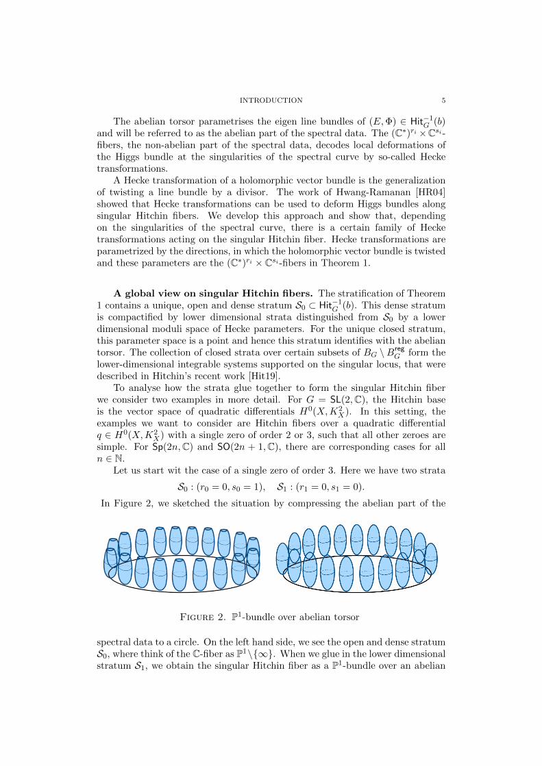


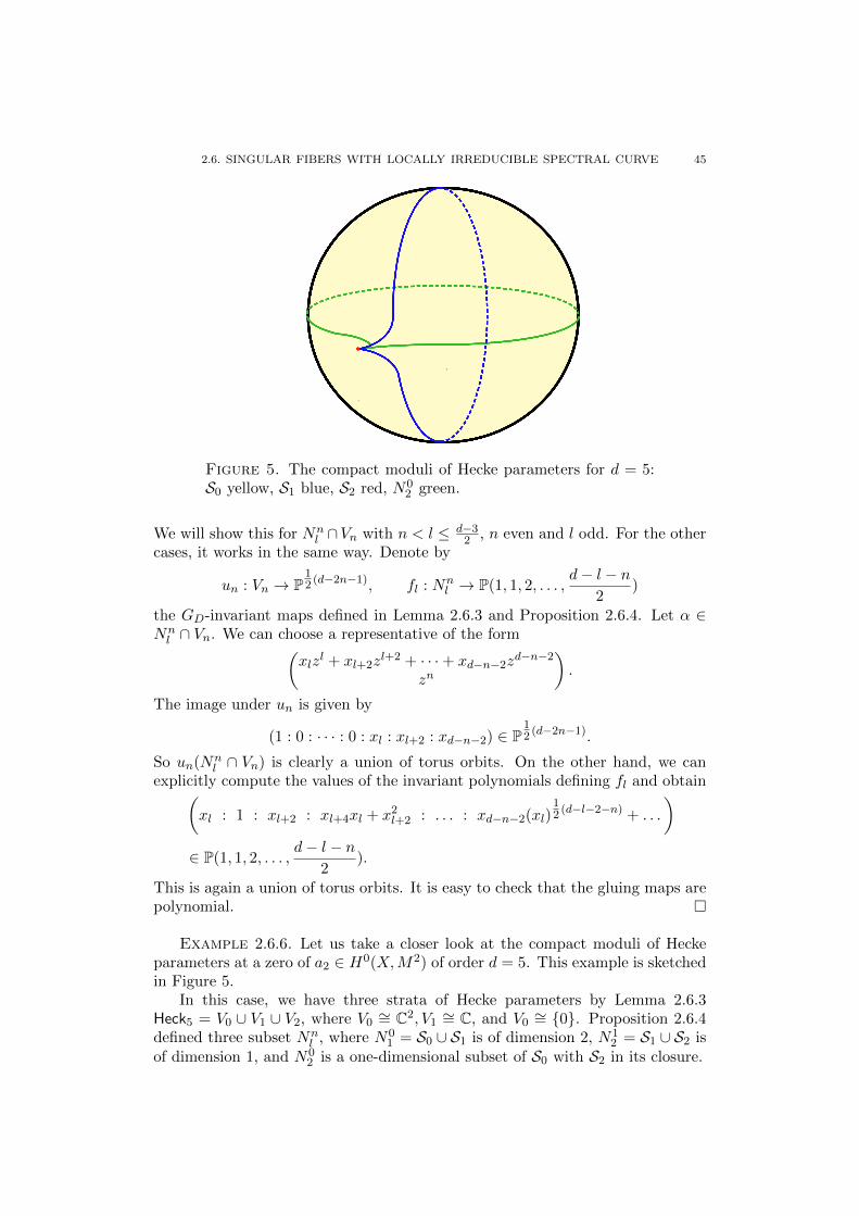


![[Hitchin N.] Differentiable Manifolds(BookZZ.org)](https://static.documents.pub/doc/80x56/55cf903b550346703ba416cf/hitchin-n-differentiable-manifoldsbookzzorg.jpg)


