Introduction Classification of surfaces Visualization Detection of singularities

Singularities of algebraic curves and surfaces— classification and detection

An overview of Work Packages 4.1 and 4.2in the GAIA II project

presented byPal Hermunn Johansen and Ragni Piene

University of Oslo

September 15, 2005

Introduction Classification of surfaces Visualization Detection of singularities

Outline

Introduction

Classification of surfaces

Visualization

Detection of singularities

Introduction Classification of surfaces Visualization Detection of singularities

Algebraic geometry and CAGD

In order to use algebraic curves and surfaces efficiently in CAGD,we need to know about their shape:

I number of connected components

I selfintersections

I other singularities

The aim would be to have a “catalogue” of surfaces (or surfacepatches) from which a CAGD person could choose models, orcandidates for approximate solutions to implicitization problems.

In short, we need to classify algebraic curves and surfaces. Whatare the tools provided by algebraic geometry?

Introduction Classification of surfaces Visualization Detection of singularities

Classification problems are classical in algebraic geometry :-)but

I most known results are only valid for projective varietiesdefined over the complex numbers :-(

I classification over the real numbers is much harder :-(

I classification in affine space is in some sense harder than inprojective space :-(

Example: the classification of conic sections.The curves x2 + y2 = 1 and x2 − y2 = 1 are not equivalent in R2,but they are equivalent (via y 7→ iy) in C2 and (via x↔ z) inP2(R).

Introduction Classification of surfaces Visualization Detection of singularities

Algebraic surfaces

The (only?) interesting algebraic surfaces from a CAGD point ofview are parameterizable (i.e., rational).

Examples are

I triangle (= Veronese) surfaces

I tensor (= Segre) surfaces (cf. Thi Ha Le’s talk)

I monoid surfaces (cf. Johansen’s talk)

I Hirzebruch and Del Pezzo surfaces (e.g. cubic surfaces)

I other toric and almost toric surfaces

I rational scrolls

I tangent developables of rational space curves.

Introduction Classification of surfaces Visualization Detection of singularities

Singularities of triangle surfaces

A triangle (or Veronese) surface is the image of

ϕ: P2 → P3,

where ϕ = (f0, f1, f2, f3), with fi homogeneous of degree d.The degree of the (implicit) equation of the image surface is ≤ d2

(equality if no base points).

Curve of selfintersection has degree

m ≤ (d4 − 4d2 + 3d)/2.

In general, this is an equality, and additional singularities are triplepoints and pinch points, whose numbers are also determined by d.

Introduction Classification of surfaces Visualization Detection of singularities

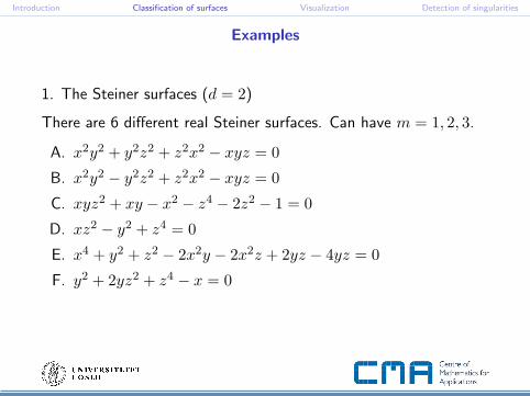
Examples

1. The Steiner surfaces (d = 2)

There are 6 different real Steiner surfaces. Can have m = 1, 2, 3.

A. x2y2 + y2z2 + z2x2 − xyz = 0

B. x2y2 − y2z2 + z2x2 − xyz = 0

C. xyz2 + xy − x2 − z4 − 2z2 − 1 = 0

D. xz2 − y2 + z4 = 0

E. x4 + y2 + z2 − 2x2y − 2x2z + 2yz − 4yz = 0

F. y2 + 2yz2 + z4 − x = 0

Introduction Classification of surfaces Visualization Detection of singularities

Introduction Classification of surfaces Visualization Detection of singularities

A: Steiner’s Roman surface. Three real double lines meeting in atriple point. Each line has two real pinchpoints. (d = 4, m = 3,t = 1, ν2 = 6)B: Three real double lines meeting in a triple point. One line hastwo real pinch points. (d = 4, m = 3, t = 1, ν2 = 2)C: One real double line. The line has one real pinch point. (d = 4,m = 1, ν2 = 1)D: One simple and one double double lines meeting in a triplepoint. The simple line has two real pinch points. (d = 4, m = 2,t = 1, ν2 = 2)E: Somewhat similar to D.F: One threefold double line containing a triple point.

Introduction Classification of surfaces Visualization Detection of singularities

2. The double pillow (d = 3)

x4 − 2x2y2 + y4 − 2x2w2 − 2y2w2 − 16z2w2 + w4 = 0

Picture in xyz-space (w = 1):

x4 − 2x2y2 + y4 − 2x2 − 2y2 − 16z2 + 1 = 0

Introduction Classification of surfaces Visualization Detection of singularities

Picture in xyw-space (z = 1):

x4 − 2x2y2 + y4 − 2x2w2 − 2y2w2 − 16w2 + w4 = 0

Introduction Classification of surfaces Visualization Detection of singularities

The dual surface of the double pillow:

16x2 − y4 + 2y2z2 − 8x2y2 − z4 − 8x2z2 − 16x4 = 0

Introduction Classification of surfaces Visualization Detection of singularities

Singularities of tensor surfaces

A tensor (or Segre) surface is given by

ϕ: P1 × P1 → P3,

where ϕ = (f0, f1, f2, f3), with fi bihomogeneous of bidegree(a, b).The degree of the (implicit) equation of the image surface is≤ 2ab. Equality if no base points.

The curve of selfintersection has degree

m ≤ 2a2b2 − 4ab + a + b.

In general, this is an equality, and additional singularities are triplepoints and pinch points, whose numbers are also determined by aand b.

For the case a = 1, b = 2, cf. the talk by Thi Ha Le.

Introduction Classification of surfaces Visualization Detection of singularities

Real versus complex

The formulas for the degree of the singular loci are essentiallygeneralized Plucker formulas. Need refined versions, treating onlythe real singular loci.

Curves: Klein showed that at most one third of the flexes of aplane curve can be real. Generalizations by Shuh, Wall.

Surfaces: Viro has some results for surfaces, but harder to interpretand to use. Generalizations by Ernstrom.

Reality questions: the number of real solutions is bounded by thenumber of complex solutions — when is the maximum achieved?

Introduction Classification of surfaces Visualization Detection of singularities

Singularities and deformations

Deformation theory exists mainly for complex varieties. FromCAGD point of view, the interesting, but more difficult, cases arethe real case, especially the affine case and the bounded case.

When a curve or surface acquires or loses a singularity, both localand global shape change.

Classification of isolated singularities: start with some coarsenumerical invariant, like multiplicity or modularity.

Modularity tells about how many different singularities can be “thesame” without being equivalent. The simplest are the simplesingularities: Ak, Dk, E6, E7, E8.

There are several definitions of “equivalent”: e.g. topological oranalytical equisingularity, and in the real case, there are differenttypes.

Introduction Classification of surfaces Visualization Detection of singularities

Arnold has classified all singularities up to a certain complexity.Each has a normal form (cf. Johansen’s talk).

For example, the normal form for Ak is x2 ± y2 − zk+1.

The A2 singularity can have two real types:

A+2 :x2 + y2 − z3 = 0 A−2 :x2 − y2 − z3 = 0

Introduction Classification of surfaces Visualization Detection of singularities

Here are two Q10 singularities:

x3 + y2z + z4 + xz3 = 0 x3 + y2z − z4 + xz3 = 0

The index 10 is the Milnor number. A finer invariant is the Tjurinanumber.

Introduction Classification of surfaces Visualization Detection of singularities

Moduli spaces

The space of all plane curves, or all surfaces in 3-space, of a givendegree can be identified with the space of the coefficients of theirequations.

E.g., the space of conics has dimension 5, the space of cubicsurfaces has dimension 20. Over the complex numbers, all conicsare equivalent, so the dimension of the moduli space of complexconics is 0. But the moduli space is more interesting for real affineconics — and gets more interesting, and much more complicated,for curves and surfaces of higher degree.

Introduction Classification of surfaces Visualization Detection of singularities

For parameterizable varieties (not necessarily hypersurfaces) wecan look at the space of parameterizations instead of the space of(implicit) equations. Taking equivalence classes of maps, we get asmaller dimensional moduli space.

This can e.g. be done for patches of tensor surfaces (cf. Thi HaLe’s talk).

More generally, want to find small dimensional families containingenough interesting objects. For example, when looking for possiblesolutions to (approximate) implicitization problems, want to get(very) sparse matrices in the elimination process.

Introduction Classification of surfaces Visualization Detection of singularities

Fast visualization of surfaces

To get a quick understanding of the shape of a given surface ofdegree d, make its equation f(x, y, z) to be monic in z. Computethe resultant R0(x, y) and certain subdeterminants Ri of theresultant matrix, i = 1, ..., d− 2. These are the Sturm–Habichtcoefficients.

The arrangement of the curves Ri = 0 in the wanted region in thexy-plane gives regions (surface patches, curves, and points) wherethe number of real solutions in z to f(x, y, z) = 0 is constant.The curve R0(x, y) = 0 is the projection of the contour of thesurface viewed from the center of projection.

The contour curve is the intersection of the surface with its firstpolar surface w.r.t. the projection center. The theory of real polarvarieties should be pursued, both in the global and local case.

Introduction Classification of surfaces Visualization Detection of singularities

Example: the double pillow

In the w = 1 case: The arrangement is given by the curve R0 = 0,which is

x4 − 2x2y2 + y4 − 2x2 − 2y2 + 1 = 0

This gives the four lines ±x± y = 1.For points (x, y) on the lines, there is one solution in w, for pointsin the four cones, there are two solutions, and for points in the restof the plane there are no real solutions.

In the z = 1 case: R0 = 0 gives the lines x + y = 0 and x− y = 0,whereas neither R1 = 0 nor R2 = 0 has real solutions.For points (x, y) on the lines there are three real solutions in w, forpoints outside the lines there are four.

Introduction Classification of surfaces Visualization Detection of singularities

Early detection of singularities

Parameterized surfaces have singularities essentially of two kinds;cuspidal edges and selfintersections. If the parameterization hasbase points, there might also be isolated singularities.

The first can be detected on the parameterization (computing theJacobian of the parameterization), the second requires a globalanalysis.

For computing selfintersections of a Bezier bicubic surface, givetwo contributions:

I a specific sparse bivariate resultant adapted to thecorresponding elimination problem

I the use of a semi-numeric polynomial solver able to deal withlarge systems of equations with floating point coefficients.

(For bidegree (2, 2) patches, cf. the talk by S. Chau.)

Introduction Classification of surfaces Visualization Detection of singularities

Early detection of singularities is important for approximateimplicitization of a parameterized surface patch. Require that theimplicitly defined surface has (nearly) the same shape (andsingularities) as the patch it tries to approximate.

A CAGD designer will not create selfintersections or othersingularities on purpose. Singular surfaces arise from built-infunctions: offset or draft or sweep. These procedural surfacescannot be avoided.

The loops or folds may be very small and hence difficult to detect.

Can represent a procedural surface via a sampling of theparameterization domain. The parameterization can be a prioricomputed on such a sampling and eventually refined (cf. thesis ofJ.-P. Pavone).

Introduction Classification of surfaces Visualization Detection of singularities

Fast detection of singularities

Exploit the properties of polynomial representations in theBernstein basis. This representation is much more numericallystable than the monomial representation and has a directgeometric meaning in terms of control points.

Subdivison approach: based on convex hull property, for checkingthe existence of solutions in the search domain.Output: no or maybe. If maybe, subdivide the domain.Continue until a termination criterion is satisfied.

Reduction approaches contract the domain where solutions aresought. Can concentrate on the parts of the domain where theroots are. (Cannot replace completely subdivision.)

Propose a general scheme for comparing and evaluating thesemethods. New reduction technique and new preconditioning steps⇒ new reduction-subdivision solver.