SIO 210 Problem Set 3 Answerkey November 9, 2016 Due November 21, 2016 (20 points)

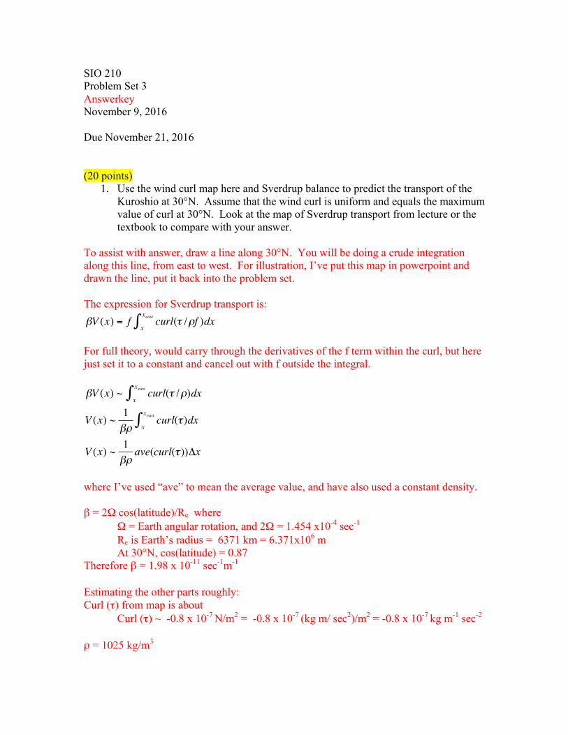
1. Use the wind curl map here and Sverdrup balance to predict the transport of the Kuroshio at 30°N. Assume that the wind curl is uniform and equals the maximum value of curl at 30°N. Look at the map of Sverdrup transport from lecture or the textbook to compare with your answer.

To assist with answer, draw a line along 30°N. You will be doing a crude integration along this line, from east to west. For illustration, I’ve put this map in powerpoint and drawn the line, put it back into the problem set. The expression for Sverdrup transport is:

€

βV (x) = f curl(τ /ρf )dxx

xeast∫ For full theory, would carry through the derivatives of the f term within the curl, but here just set it to a constant and cancel out with f outside the integral.

€

βV (x) ~ curl(τ /ρ)dxx

xeast∫

V (x) ~ 1βρ

curl(τ)dxx

xeast∫

V (x) ~ 1βρ

ave(curl(τ))Δx

where I’ve used “ave” to mean the average value, and have also used a constant density. β = 2Ω cos(latitude)/Re where

Ω = Earth angular rotation, and 2Ω = 1.454 x10-4 sec-1 Re is Earth’s radius = 6371 km = 6.371x106 m At 30°N, cos(latitude) = 0.87

Therefore β = 1.98 x 10-11 sec-1m-1

Estimating the other parts roughly: Curl (τ) from map is about

Curl (τ) ~ -0.8 x 10-7 N/m2 = -0.8 x 10-7 (kg m/ sec2)/m2 = -0.8 x 10-7 kg m-1 sec-2 ρ = 1025 kg/m3

Δx: approximately 120 ° longitude. At 30°N, 1° longitude = 111km *cos(30°) = 111 km * 0.86 = 96 km = 96 x103 m Δx ~ 120 (96 x103 m)

€

V =1

1.98x10−11 sec−1m−11

1025kgm−3 (−0.8x10−7kgsec−1m−1)(120°)(96x103m /°)

V = 45.6x106m3/sec = 45.6 Sv This number should be rounded given all the approximations. If I had used a curl(tau) of -1.0x10-7 N/m3 instead, then the value would be more like 56 Sv. So the ballpark estimate is around 50 Sv, which is similar to the Sverdrup transport in the map from lecture based on this wind stress curl.

(16 points) 2. The  California  Current  flows  southward  along  the  west  coast  of  the  U.S.    For  this  question,  consider  it  as  a  separate  phenomenon  from  the  subtropical  gyre.    The  California  Current  is  driven  by  a  southward  alongshore  wind.    The  wind  causes  an  offshore  Ekman  transport.    (It  is  also  driven  by  upwelling  due  to  offshore  strengthening  of  the  southward  wind,  but  that  is  not  part  of  this  problem.  Assume  here  that  the  wind  is  uniform  in  latitude  and  longitude.)    Assume  that  the  total  offshore  Ekman  transport  is  1  Sv.    (1  Sv  =  1x106  m3/sec.)  

 (a) Explain  how  the  California  Current  itself  arises  from  this  forcing.  (short  

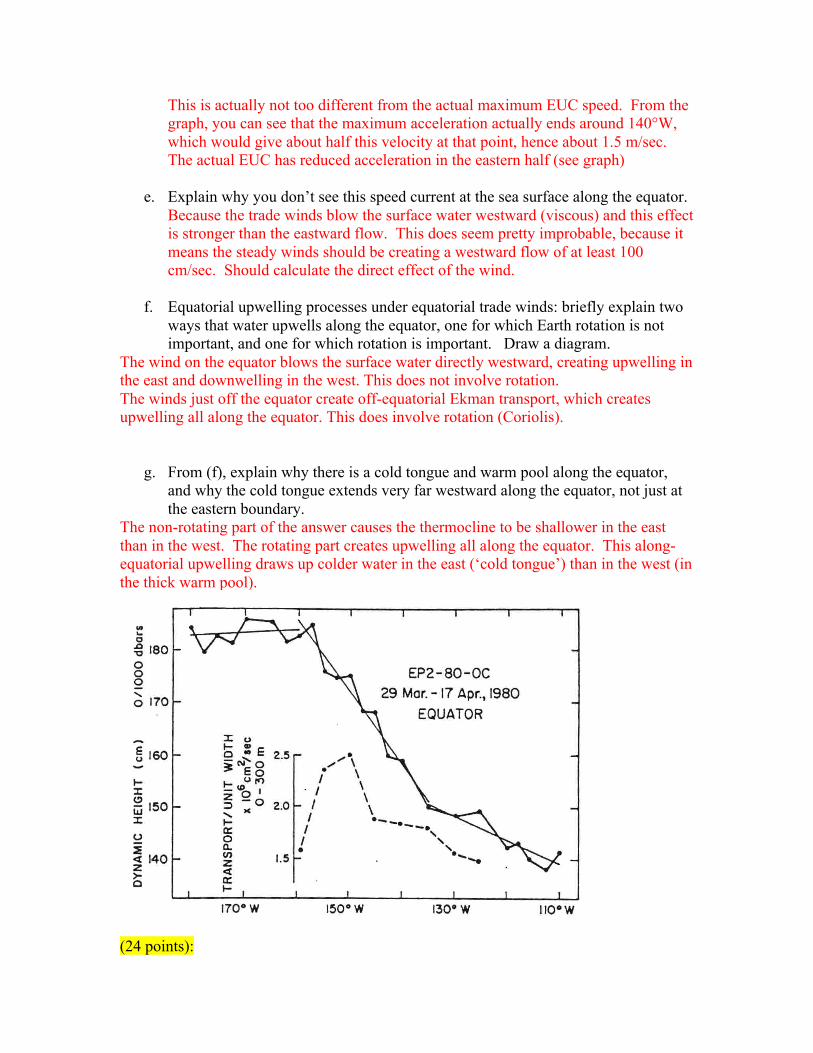
answer)  The  alongshore  wind  stress  drives  offshore  Ekman  transport,  as  stated.    This  creates  coastal  upwelling.    This  (plus  the  broad  upwelling  driven  by  the  wind  stress  curl  arising  from  strongest  winds  offshore)  causes  the  thermocline  to  rise  towards  the  coast.    It  also  piles  water  up  offshore.    The  pile  of  water  offshore  creates  an  eastward  pfg  which  drives  a  southward  geostrophic  flow  which  is  the  California  Current.  The  tilted  pycnocline  causes  this  current  to  decay  with  depth.        (b)  Along  the  coast,  there  is  upwelling  in  a  strip  that  is  about  10  km  wide.    Assume  that  it  occurs  over  a  1000  km  length  of  the  coast.      Make  a  reasonable  assumption  for  the  thickness  of  the  upwelling  layer  based  on  what  is  causing  the  upwelling.    ______100  to  no  more  than  200_________m    Assuming  that  the  Ekman  transport  of  1  Sv  occurs  out  of  this  box,  calculate  the  offshore  Ekman  velocity  (using  the  transport  and  dimensions  of  the  box)    The  cross-­‐sectional  area  for  the  transport  is    Areavert  =  1000  km  x  100  m  =  1x106  m  x  1x102  m  =  1x108  m2    The  average  velocity  is  the  Ekman  transport  divided  by  area.  uave  =  1  Sv  /  1x108  m2  =  (1  x  106  m3/sec)/(  1x108  m2)  =    =  0.01  m/sec  =  1  cm/sec      (c)  Calculate  the  upwelling  velocity  into  the  box    (using  the  transport  and  dimensions  of  the  box).  This  requires  the  surface  area  of  the  box  which  is    Areasurface  =  1000  km  x  10  km  =  104km2  =  1010m2    W  =  1  Sv  /  1x1010  m2  =  (1  x  106  m3/sec)/(  1x1010  m2)  =    1x10-­‐4  m/sec  =  10-­‐2  cm/sec   (25 points) 3. Equatorial undercurrent speed. A plot of the surface height from west to east along the equator in the Pacific, shown in class, is shown here. (The axis is labeled ‘dynamic height’ but assume that it is actual physical height.) Ignore the inset diagram.

a. Compute the pressure gradient force (“pgf”) across the whole width of the Pacific. You’ve done a similar calculation on other homework. From graph, the height difference is Δz ~ 45 cm = 0.45 m. From graph, the distance is 50° longitude. At the equator, 1° = 111 km, so the distance is Δx = 50 x 111 km = 5550 km = 5.55 x 106 m. The pgf is (-1/ρ)(Δp/Δx). Δp comes from hydrostatic balance: 0 = -(Δp/Δz) –ρg, so

Δp = –ρgΔz and therefore

pgf = (-1/ρ)(Δp/Δx) = gΔz/Δx = (9.8 m sec-2) (0.45 m)/( 5.55 x 106 m) = 7.9x10-7 m sec-2

b. Assume the ocean response to the pgf is acceleration. What direction will the pressure gradient force accelerate the flow (east, west, north, south)? To the east Why? Because at the equator, the response to the pgf is direct, since there is no Coriolis force.

c. Calculate the eastward acceleration. It is equal to the pgf = 7.9x10-7 m sec-2 d. On the chart, SSH is nearly uniform between the western side and 160°W. If the

flow starts accelerating here, how fast will it be going when it reaches the boundary? Assume that there is just one value for the pgf. (Authors have attached two slopes to the data.) This is an approximate answer as well. We know the acceleration from (c). We do not know the time. With some manipulation of the expressions for velocity and acceleration, we can approximately eliminate the time and find the approximate velocity. Assume acceleration a is constant.

To get velocity, integrate acceleration from time 0 to t at the eastern side.

Assume initial velocity u(0) = 0.

u(t) – u(0) = u(t) = aΔt so a = u(t)/Δt Because accelearation is constant, u changes uniformly, and the velocity at the eastern side u(t) is twice the average velocity uave.

uave = Δx/Δt and uave = u(t)/2 so Δt = Δx/ uave = 2Δx/ u(t) Substitute this Δt into the expression for acceleration: a = u(t)/Δt = u2(t) /(2Δx) and u(t) = sqrt(2a Δx) Substitute in values: a = du/dt = Δu/Δt = 7.9 x10-7 m/sec2

Δx = 5.55 x 106m So u(t) = sqrt(2a Δx) = sqrt(2 * 7.9 x10-7 m/sec2 * 5.55 x 106m) = 2.96 m/sec

This is actually not too different from the actual maximum EUC speed. From the graph, you can see that the maximum acceleration actually ends around 140°W, which would give about half this velocity at that point, hence about 1.5 m/sec. The actual EUC has reduced acceleration in the eastern half (see graph)

e. Explain why you don’t see this speed current at the sea surface along the equator.

Because the trade winds blow the surface water westward (viscous) and this effect is stronger than the eastward flow. This does seem pretty improbable, because it means the steady winds should be creating a westward flow of at least 100 cm/sec. Should calculate the direct effect of the wind.

f. Equatorial upwelling processes under equatorial trade winds: briefly explain two

ways that water upwells along the equator, one for which Earth rotation is not important, and one for which rotation is important. Draw a diagram.

The wind on the equator blows the surface water directly westward, creating upwelling in the east and downwelling in the west. This does not involve rotation. The winds just off the equator create off-equatorial Ekman transport, which creates upwelling all along the equator. This does involve rotation (Coriolis).

g. From (f), explain why there is a cold tongue and warm pool along the equator, and why the cold tongue extends very far westward along the equator, not just at the eastern boundary.

The non-rotating part of the answer causes the thermocline to be shallower in the east than in the west. The rotating part creates upwelling all along the equator. This along-equatorial upwelling draws up colder water in the east (‘cold tongue’) than in the west (in the thick warm pool).

(24 points):

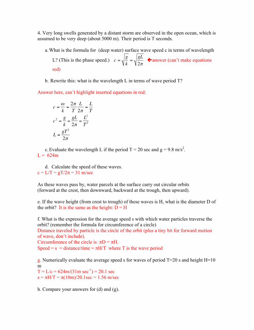
4. Very long swells generated by a distant storm are observed in the open ocean, which is assumed to be very deep (about 5000 m). Their period is T seconds.

a. What is the formula for (deep water) surface wave speed c in terms of wavelength

L? (This is the phase speed.)

€

c =gk

=gL2π

!answer (can’t make equations

red)

b. Rewrite this: what is the wavelength L in terms of wave period T? Answer here, can’t highlight inserted equations in red:

€

c =ωk

=2πT

L2π

=LT

c 2 =gk

=gL2π

=L2

T 2

L =gT 2

2π

c. Evaluate the wavelength L if the period T = 20 sec and g = 9.8 m/s2.

L = 624m

d. Calculate the speed of these waves. c = L/T = gT/2π = 31 m/sec As these waves pass by, water parcels at the surface carry out circular orbits (forward at the crest, then downward, backward at the trough, then upward). e. If the wave height (from crest to trough) of these waves is H, what is the diameter D of the orbit? It is the same as the height: D = H f. What is the expression for the average speed s with which water particles traverse the orbit? (remember the formula for circumference of a circle) Distance traveled by particle is the circle of the orbit (plus a tiny bit for forward motion of wave, don’t include). Circumference of the circle is πD = πH. Speed = s = distance/time = πH/T where T is the wave period g. Numerically evaluate the average speed s for waves of period T=20 s and height H=10 m T = L/c = 624m/(31m sec-1) = 20.1 sec s = πH/T = π(10m)/20.1sec = 1.56 m/sec h. Compare your answers for (d) and (g).

The speed of actual particles in the waves, going around their orbit, is much smaller than the speed of the wave through the water. s = 1.56 m/sec while c = 31 m/sec (15 points) 5. Short answer questions about tides. For each

(i) mark the most nearly correct answer (1 point) (ii) write a brief explanation of your answer. (2 points) (iii) draw a small diagram to illustrate your answer. (2 points)

a. Spring tides (times of large semidiurnal tidal range) occur twice a month

A. when the moon is in the earth's equatorial plane, B. when the moon is out of the earth's equatorial plane, C. at full or new moon, D. at the quarter moons, E. at lunar perigee.

During full and new moon, the moon and sun are aligned, which increase the gravitational attraction and therefore increases the size of the tide. I have inserted the diagram from the SIO210 CSP lecture that illustrates the spring tide, when moon and sun are aligned; the other spring tide is when the moon is opposite the sun because the tidal bulges are equal and opposite for both the moon and sun attraction.

b. The daily inequality (elevation difference between a high tide and its immediate successor) vanishes for lunar tides

A. when the moon is in the earth's equatorial plane, B. when the moon is out of the earth's equatorial plane, C. at full or new moon, D. at the quarter moons, E. at lunar perigee.

The daily inequality arises from the moon being out of the equatorial plan, so that when a given location rotates under the moon, say, one high tide bulge is closer to the plane of the moons’ orbit than the other. I have inserted the diagram from the SIO210 CSP lecture that illustrates the daily inequality that occurs when the moon is NOT in the equatorial plane.

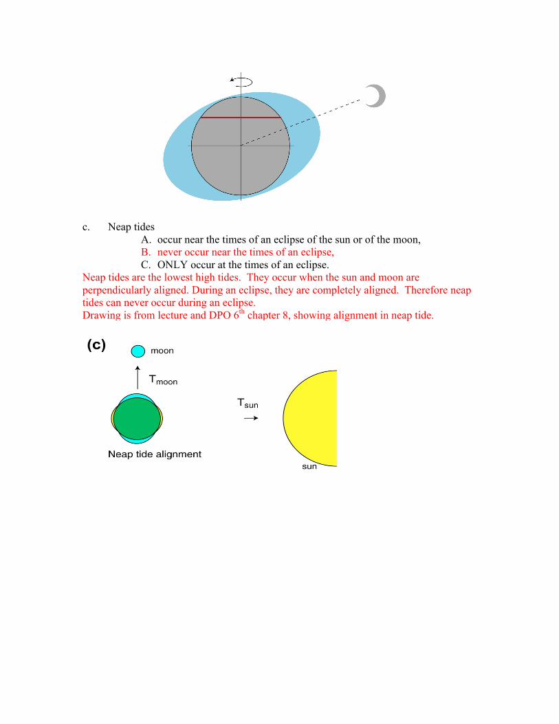
c. Neap tides

A. occur near the times of an eclipse of the sun or of the moon, B. never occur near the times of an eclipse, C. ONLY occur at the times of an eclipse.

Neap tides are the lowest high tides. They occur when the sun and moon are perpendicularly aligned. During an eclipse, they are completely aligned. Therefore neap tides can never occur during an eclipse. Drawing is from lecture and DPO 6th chapter 8, showing alignment in neap tide.