Page 1
205
Pakistan Economic and Social Review Volume 54, No. 2 (Winter 2016), pp. 205-231
SIZE AND IMPACT OF FISCAL MULTIPLIERS
An Analysis of Selected South Asian Countries
MUHAMMAD AZMAT HAYAT AND HAFSAH QADEER*
Abstract. Due to recent global financial and economic crisis a key issue
in current research and for policy makers is the size of fiscal multipliers.
Proper knowledge of fiscal multipliers is essential for the designing and
implementation of fiscal policies. This research work intends to contribute
in the literature on the size of fiscal multipliers for selected South Asian
countries (Bangladesh, India, Pakistan and Sri Lanka) by using Panel
Vector Autoregressive (PVAR) technique over the period 1982-2014.
Results obtained from accumulated Impulse Response Functions (IRFs)
show that government expenditures have overall positive impact on output
in these countries. Among expenditures government investment
multipliers are greater than government consumption multipliers on all
time horizons. This finding suggests that governments should put more
emphasis on public investment while allocating budget in these countries.
When controlling for public debt, cumulative fiscal multipliers exhibit
lower values. Additionally, the results also show that during business
cycle phases government expenditures show more efficacies in recessions
while lower effect in expansions.
Keywords: Fiscal multipliers, Panel vector autoregressive, Impulse response function, Government expenditures, Business cycles
JEL classification: C32, E32, E62
I. INTRODUCTION
Many economists are of the view that macroeconomic stabilizations should
be handled mainly by monetary policy (Farhi and Werning, 2012). But
*The authors are, respectively, Assistant Professor and M. Phil. Scholar at the Department
of Economics, University of the Punjab, Lahore-54590 (Pakistan).
Corresponding author e-mail: [email protected]
Page 2
206 Pakistan Economic and Social Review
unfortunately monetary policy is not free from constraints that restrict its
efficiency. For example, the economy may entrap into the situation of
liquidity trap (close to lower bound interest rate scenario) that prohibit
further reduction in interest rates. Furthermore, there are many countries that
belong to currency unions (like European countries, Eastern Caribbean
Currency Union (ECCU) etc.) or states with in the country don’t have the
choice of independent monetary policy (Farhi and Werning, 2012).
The latest worldwide economic crisis had brought the attention of
authorities towards the usefulness of fiscal policy for two reasons: the first
argument was that during that time, the credit and monetary policy had hit its
lower limit (a situation of zero lower bound interest rate),1 in this situation
there is no choice for policy makers to rely on the fiscal policy for
stimulating economic activity and employment during the period of slump.
The second argument was that it was expected to have long lasting
recessionary phases across the countries. In this situation, fiscal stimulus
regardless of its conventional lags in implementation would have adequate
time to give positive results and stable the economy.
The most important channel through which global financial crisis (GFC)
hit the economies of South Asia was exports. The United States and
European economies were major markets for the exports of South Asian
countries. There was a sharp decline in the growth of exports of the South
Asian countries due to a sharp decline in demand in the Western economies.
TABLE 1
Growth of Exports Demand, Annual Change, Percentage
Countries 2006 2007 2008 2009 2010 2011 2012 2013 2014
Bangladesh 25.5 13.0 7.1 0.0 0.9 29.3 12.5 2.5 3.2
India 20.4 5.9 14.6 –4.7 19.6 15.6 6.7 7.3 –0.8
Pakistan 9.9 1.5 –4.6 –3.4 15.7 2.4 –15.0 13.6 –1.6
Sri Lanka 3.8 7.3 0.4 –12.3 8.8 11.0 0.2 5.9 4.9
Source: Asian Development Bank, Key Indicators for Asia and the Pacific 2015.
The recent crisis was due to the shortage of demand. During zero
interest rate situations the basic goal of a policy should not be to increase
1By the end of 2008, the short-run nominal interest rate which is the main operating tool of
monetary policy had reached to its very low value regarding to an effective lower bound
by the central bank.
Page 3
HAYAT and QADEER: Size and Impact of Fiscal Multipliers 207
aggregate supply by providing aggregate supply incentives. Instead the goal
of a policy should be to boost up the overall spending of an economy, i.e.
aggregate demand. Output is demand determined at zero interest rate
situations. Correspondingly, aggregate supply is usually relevant in the
model because it talks about future inflation from the expectations of people.
Therefore, we can say that the policies that are formulated to boost up the
aggregate supply are counter-productive because at zero interest rate they
can create deflationary pressure in an economy. So, as a consequence of this
policy makers should not formulate such policies that increase the supply of
goods when the problem is that there are not much buyers (Eggertsson,
2011). Fiscal policy has an advantage over monetary policy, that increase in
government spending can immediately increase the aggregate demand.
From 2008-2009, both the developed and developing nations has
undertaken various fiscal policy stimuli to boost the declining economy. It is
not possible to access the impact of the fiscal policy on economic growth
without proper study on the size, sign and the magnitude of the fiscal
multipliers. Moreover, size of expenditure (spending) multipliers also
portrays the quality and effectiveness of fiscal policy. These factors and also
the lack of empirical estimations on the size of fiscal multipliers for a panel
of South Asian economies (Pakistan, India, Bangladesh and Sri Lanka) have
been a source of motivation behind this study. This research tries to
investigate the size and sign of government expenditures and government
revenue (taxes) multipliers for selected South Asian countries. This study
also tries to estimate the effect of debt dynamics and business cycle phases
(recession and expansion) on the magnitude of fiscal multipliers.
This research paper is structured as follow: Section II discusses the
theoretical mechanism behind fiscal multipliers; Section III reviews the
background literature; Section IV discusses the data and methodology;
Section V discusses the estimation and results and in section VI conclusion
and policy implications are discussed.
II. THEORETICAL MECHANISM BEHIND
FISCAL MULTIPLIERS
Initially the concept of “multiplier” was introduced by Kahn (1931) and then
further elaborated by Keynes (1936). According to Keynes-Kahn textbook
version of multipliers if public expenditure (G) increases by one unit, as a
consequence of this aggregate demand increases by more than one unit. The
initial round of spendings stimulate the next rounds of spending in this way
the final impact on output is multiplier times the original increase in
Page 4
208 Pakistan Economic and Social Review
spending. If the initial increase in public spending is ∆G and marginal
propensity to consume (MPC) is “c” then change in output is k times ∆G,
where k is the fiscal multiplier and equals k = 1 / (1 – c) and for taxes it is
given by –MPC / (1 – MPC), under the assumption of close economy. The
value of multiplier is the accumulated effect on output through various
rounds of spending2 (Bose and Bhanumurthy, 2015).
In simple terms fiscal multiplier refers to the ratio of change in output
due to some exogenous change in fiscal instrument – such as government
expenditures or government taxes. There are several types of fiscal
multipliers depending on different time horizons. Impact multiplier is the
ratio of change in output (at time t0) due to an exogenous change in the fiscal
variable at time t0, i.e. ∆Yt0 / ∆Gt0. Cumulative multiplier is defined as the
ratio of cumulative change in output due to cumulative exogenous changes in
the fiscal variables. ∆Yt0 + i / ∆Gt0 + N where i = 0, 1, …, N.
In the case of zero lower bound (ZLB) interest rate situation the
multiplier for output is greater than unity. The whole mechanism behind this
result is that government spending promotes inflation in an economy. As the
nominal interest rate is fixed, this reduces the real interest rate which
motivates the investors to enhance their investment (their current spending).
The increase in consumption in turn of this leads to more inflation, in this
way it creates a feedback loop. The fiscal multiplier is increasing in the
degree of price flexibility. The whole mechanism relies on the response of
inflation (Farhi and Werning, 2012). The core thinking behind taking these
policy actions are that both recession and inflation are opposite of one
another. During periods of inflation there is too much money circulating in
an economy, but during the phases of recession there is not enough money.
So during recessionary phases in order to put money in the economy
government increases its expenditures to create inflationary situation in the
economy.
Many macroeconomics models predict that a rise in government
spending will have an expansionary effect on aggregate output; these models
are generally differing according to their implicit effect on consumption. As
the later variable (consumption) is the largest component of aggregate
demand, its response is the crucial determinant about the size and sign of
government spending multiplier.
2[1 / (1 – c)] is the summation of the series c + c2 + c3 + …. ∞, i.e. additions through
multiplier rounds.
Page 5
HAYAT and QADEER: Size and Impact of Fiscal Multipliers 209
The weak Keynesian and IS-LM model predict that consumption will
increase after a shock in government spending. In these models MPC is high
because consumers are not forward looking and they do not fully consider
that in future taxes will increase to compensate for current increase in debt
and increase in government spending due to their finite horizon. In other
words, in the IS-LM model consumers behave in a non-Ricardian fashion,
i.e. rule of thumb consumers. From another perspective when a shock in
government spending is given its effect on output is weaken due to domestic
crowding out effects from investment for a large economy, although in a
small but financially integrated economy the size of the fiscal multiplier is
further curtailed due to negative effect of real exchange rate on foreign
demand and marginal propensity to imports.
The Real Business Cycle (RBC) models are considered as the stochastic
versions of the Classical Models. The characteristics of these models are the
presence of micro foundations and intertemporal considerations. The RBC
model has infinitely lived and forward looking behaviour consumers with no
nominal rigidities and whose consumption decision are based on
intertemporal considerations. In these models positive government spending
shock will have a negative wealth effect and this positive shock reduces the
consumption in favour of saving while increase the labour supply and have a
negligible increase in output. Hence, reduction in tax has no effect on
consumption and on income. This reduction in tax is usually portrayed as
Ricardian equivalence (Barro, 1974). On the other hand, a tax shock that is
not followed by any discretionary changes in government spending have no
effect on output, because this lower tax today will be balanced by higher
future taxes and in this way present discounted value will remain unchanged
(Ricardian Equivalence). But when government spending is financed by
distortionary taxes, then both social welfare and output level will be reduced,
therefore giving a negative value of government spending multiplier.
Summing up we can say that different types of models will give us
different magnitudes of the multipliers. The reason of the difference of the
impact of fiscal variables across these models lies in the fact of how
consumers behave in each model. In addition to this, the size of multiplier
also depends seriously on the conduct of monetary policy, level of public
debt, trade openness, exchange rate regimes, uncertainty and saving rate.
Taxes and public expenditure/spending multipliers are key parameters
for accessing the effectiveness of fiscal policy in managing output
fluctuations. These multipliers provide a quantitative measure of change in
output as a result of increase in taxes or spendings.
Page 6
210 Pakistan Economic and Social Review
An estimation of the size and the sign of the fiscal multipliers are essen-
tial for the designing and implementation of fiscal policies. If a government
spending multipliers are smaller than expected, then expansionary fiscal
policy will be failed to boost the economic activity of a country sufficiently
and it will also increase the public indebtedness (along with associated debt
service) as a percentage of GDP. The second important component of fiscal
policy is taxes (revenue side) a tax multiplier that have a larger than expected
(more negative) value may depress the economic activity more than
anticipated and it will sooner or later destroy the tributary base from which
all the taxes are collected (Gonzalez-Garcia et al., 2013).
III. REVIEW OF LITERATURE
The topic of fiscal multipliers again gets attention from the policy makers
and economists, due to recent crisis. Therefore modern literature on this topic
has grown rapidly and most of the empirical work uses VAR framework for
the estimation of fiscal multipliers. This research tries to give a very selective
overview of the most important issues and results.
According to economic theory government spending has positive effect
on stimulating the aggregate demand for an economy. Marattin and Salotti
(2011) found that increase in government spendings had a significantly
positive effect on private consumption and private investment for European
Union (EU) from 1970-2006, but these effects died out gradually (faster in
the case of private consumption). Jamec et al. (2011) used quarterly data of
Solvenia for taxes and government spending from 1995:1 to 2010:4. They
found positive government spending shocks had positive effect on output,
private consumption and investment on impact, but shocks became
insignificant for next periods. On the other hand, tax shocks had negative
effect on impact and shock also became insignificant in next periods. Bose
and Bhanumurthy (2015) estimated positive expenditure multipliers from
1991-2012 for Indian economy where tax multipliers were in the range of –1.
On the same lines Silva et al. (2013) accessed public spendings had a
negative effect on output on impact but cumulative effect was positive. On
the other hand, taxes had overall negative effect on output, for a panel of
Euro area from 1998-2008. For Mediterranean countries Minea and Mustea
(2015) analyzed positive and significant respond of output on impact by
giving shock in government consumption and investment. But after one year
government investment became three times larger than government
consumption multipliers.
Page 7
HAYAT and QADEER: Size and Impact of Fiscal Multipliers 211
Studies also show that fiscal multipliers are small and short lived for
instance, Trezzi et al. (2010) estimated short lived and small fiscal
multipliers for Argentina, based on the data from 1993Q4-2004Q3. On the
same pattern Parkyn and Vehbi (2014) investigated positive but small fiscal
multipliers for short-run in the case of New Zealand. These small and short-
lived multipliers might be due to some leakages from the economies. As
Espinoza and Senhadji (2011), Silva et al. (2013) and Gonzalez-Garcia et al.
(2013) accessed weak and below unity value of multipliers due to substantial
leakages through remittances, imports and degree of openness.
According to available literature, business cycle phases also affect the
size of fiscal multipliers. Many studies support the fact that fiscal multipliers
are countercyclical in nature, for instance; Bachmann and Sims (2012)
checked the effect of confidence as a transferring channel of fiscal policy
shocks into economic activities for US data. They found that confidence
level turned the size of multipliers larger in recessions than those in
expansions, especially when cumulative effect on output was considered. On
the same lines, Auerbach and Goronichenk (2013) estimated larger
multipliers for recessions while smaller even negative for expansions but not
statistically different from zero for large number of OECD countries from
1985-2010. Baum et al. (2012) found larger government spending and
revenue multipliers when output gap was negative as compared to positive
output gaps for six of G7 economies. De Cos and Moral-Benito (2016)
accessed specific multipliers for Spain that depend upon conditions of public
finances, the health of banking sector and the business cycle by using data
from 1986-2010. They estimated spending multipliers were around 1.4
during crises situations and 0.6 during normal times. In a study closer to
ours, Silva et al. (2013) also investigated positive spending multipliers for
recessions and smaller even negative for expansions. Chouliarakis et al.
(2013) found that during negative output gap the impact multipliers was
above 0.5 (and also significant) and during positive output gap the value of
spending multipliers was very low and statistically insignificant.
Exchange rate regimes also affect the size of fiscal multipliers as Ilzetzki
et al. (2013) and Chouliarakis et al. (2013) found larger multipliers for
economies having fixed exchange rates than that of floating exchange rate
regimes.
Fiscal multipliers also vary from country to country and it depends upon
different characteristics of the countries for instance, empirical estimations of
Ilzetzki et al. (2013) for 144 countries (24 are developing countries) from
1960-2007 showed that government consumption multipliers were larger in
Page 8
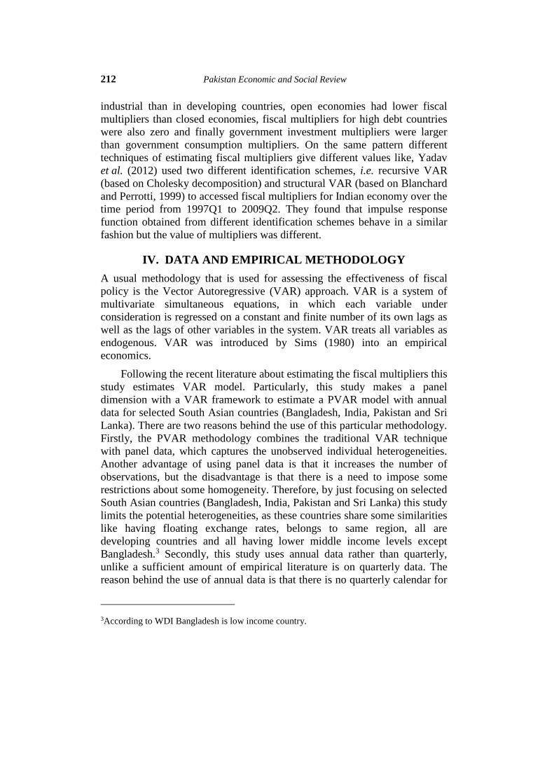
212 Pakistan Economic and Social Review
industrial than in developing countries, open economies had lower fiscal
multipliers than closed economies, fiscal multipliers for high debt countries
were also zero and finally government investment multipliers were larger
than government consumption multipliers. On the same pattern different
techniques of estimating fiscal multipliers give different values like, Yadav
et al. (2012) used two different identification schemes, i.e. recursive VAR
(based on Cholesky decomposition) and structural VAR (based on Blanchard
and Perrotti, 1999) to accessed fiscal multipliers for Indian economy over the
time period from 1997Q1 to 2009Q2. They found that impulse response
function obtained from different identification schemes behave in a similar
fashion but the value of multipliers was different.
IV. DATA AND EMPIRICAL METHODOLOGY
A usual methodology that is used for assessing the effectiveness of fiscal
policy is the Vector Autoregressive (VAR) approach. VAR is a system of
multivariate simultaneous equations, in which each variable under
consideration is regressed on a constant and finite number of its own lags as
well as the lags of other variables in the system. VAR treats all variables as
endogenous. VAR was introduced by Sims (1980) into an empirical
economics.
Following the recent literature about estimating the fiscal multipliers this
study estimates VAR model. Particularly, this study makes a panel
dimension with a VAR framework to estimate a PVAR model with annual
data for selected South Asian countries (Bangladesh, India, Pakistan and Sri
Lanka). There are two reasons behind the use of this particular methodology.
Firstly, the PVAR methodology combines the traditional VAR technique
with panel data, which captures the unobserved individual heterogeneities.
Another advantage of using panel data is that it increases the number of
observations, but the disadvantage is that there is a need to impose some
restrictions about some homogeneity. Therefore, by just focusing on selected
South Asian countries (Bangladesh, India, Pakistan and Sri Lanka) this study
limits the potential heterogeneities, as these countries share some similarities
like having floating exchange rates, belongs to same region, all are
developing countries and all having lower middle income levels except
Bangladesh.3 Secondly, this study uses annual data rather than quarterly,
unlike a sufficient amount of empirical literature is on quarterly data. The
reason behind the use of annual data is that there is no quarterly calendar for
3According to WDI Bangladesh is low income country.
Page 9
HAYAT and QADEER: Size and Impact of Fiscal Multipliers 213
the revision of fiscal policy and usually major fiscal policy decisions are
taken at the start of new fiscal year and hence due to this reason annual
interpretation of fiscal shocks may be facilitated (Marattin and Salotti, 2011).
Data on real variables are collected on annual basis in billions of dollars
from 1982-2014 for a panel of four South Asian countries from Asian
Development Bank (ADB),4 International Financial Statistics (IFS) and
World Development Indicators (WDI).
In order to make empirical estimation first of all this study will estimate
average fiscal multipliers from taxes and government expenditures and
afterward estimates disaggregated fiscal multipliers by just considering
different items on expenditure sides.
THE PVAR MODEL
On the basis of recent literature, structural version of our model can be
written as, indexing countries as i = 1, 2, …, N and time as t = 1, 2, …, T.
Azit = Λ0 + Λ1zit–1 + it (1)
where
zit = vector of endogenous variables of the model (namely
government expenditures, revenues, GDP)
A = matrix described simultaneous relationship between variables.
Λ1 = matrix of coefficient of lagged variables.
it = vector of errors.
Multiplying equation (1) by the inverse of matrix A, namely A–1 we
obtain equation (2)
Azit (A–1) = Λ0 A
–1 + Λ1 A–1
zit–1 + it A–1 (2)
Suppose:
Λ0 A–1 = 0
Λ1 A–1 = 1
it A–1 = eit
The reduced form of above system, which is actually estimated, is
expressed as
4Key indicators for Asia and the Pacific 2014.
Page 10
214 Pakistan Economic and Social Review
zit = 0 + 1 zit–1 + eit (3)5
In this scenario of rapid growth and development, it is very difficult task
for any nation to finance its all development expenses with its own domestic
resources. Therefore, accumulation of external debt is a common
phenomenon of almost all developing countries. In spite of its positive
impact a major consensus of economist is that debt is a burden on a nation.
In order to control the effect of debt on the growth of GDP, this study
considers the debt as an exogenous variable. Usually exogenous terms are
not included in VAR models, but Lütkepohl (2005) introduces exogenous
variables in the VAR (p). So the above reduced form equation after adding
the exogenous variable (DEBT) can be written as
zit = 0 + 1 zit–1 + B0 DEBTit + eit (4)
The above equation can be estimated on a group of selected countries, it
is particularly appropriate for cases in which the time dimension of the data
is relatively limited. In addition, in every PVAR specification we include
fixed effects to account for time-invariant unobserved country heterogeneity.
In a standard form of the model, the errors et are at composites of the
white noise processes and therefore have zero means, individually serially
uncorrelated and have constant variance.
IDENTIFICATION OF THE PVAR
The interpretation of the individual parameters is difficult in VAR models.
Therefore, the practitioners of this technique often estimated the so called
IRFs. IRF describes the reaction of one variable due to a shock in another
variable in the system by holding all other shocks equal to zero. On the same
pattern this study computes the response of output by giving shock into fiscal
variables under PVAR model by using impulse response analysis. However,
the major problem that is highlighted in the literature is the identification of
the truly exogenous shocks. Due to this reason the study follows the
recursive formulation approach (Cholesky decomposition) proposed by Sims
(1980). Under recursive formulation approach arrangement of the variables
is very important. The identifying assumption behind the arrangement of the
variables is that the variables that come earlier in the ordering affects the
following variables contemporaneously, as well as with lags, but the
5This derivation help is taken from Inessa Love’s paper “Financial Development and
Dynamic Investment Behavior: Evidence from Panel Vector Autoregression”.
Page 11
HAYAT and QADEER: Size and Impact of Fiscal Multipliers 215
variables that comes later only affect the previous variables with a lag. This
arrangement of the variables actually shows the causal relationship between
the variables (Silva et al., 2013). In other words, the variables that come
earlier in the system are more exogenous and those variables that come later
are more endogenous.
For this study the chosen order of the variables are: GOVERNMENT
EXPENDITURES, GDP, and TAXES. This arrangement of the variables
means that output responds contemporaneously to changes in government
expenditures, but government expenditures does not respond contempo-
raneously by changes in output. Similarly, output has a contemporaneous
effect on tax revenues but the converse is not possible. The reason behind
this arrangement of variables is that the political process requires some
substantial delays for designing and implementation of the changes in the tax
rates, which at the margin have an effect on the output level, investment and
consumption plans also take some time to adopt to a policy even after being
enacted (Silva et al., 2013).
For disaggregated model, in which government expenditures are split
into government investment and government consumption, the arrangement
of the variables are in this way: GOVERNMENT INVESTMENT,
GOVERNMENT CONSUMPTION, GDP, and TAXES. Here constant term
and DEBT are also considered as exogenous variables. Regarding to the
specific ordering of the variables, it is decided to always order government
consumption expenditures after government investment expenditures, as it is
quite reasonable that investment generates current consumption (Gonzalez-
Garcia et al., 2013).
Debt is usually considered as a burden and debt services act as a leakage
from the economy. Therefore, a separate model is estimated in which debt is
not considered as an exogenous variable, in order to compare government
expenditure multipliers with and without controlling for debt.
Additionally, aggregated PVAR model has been separately estimated
across business cycle phases (expansions and recessions) and results of fiscal
multipliers in expansions and recessions are compared. The output gap is
used for the measurement of economic activity or “excess demand”, it is the
difference between actual and potential output. Output gap represent
business cycle fluctuations which are basically identified with deviation from
the trend of the process. In this study output gap is computed with the help of
Hoddrick-Prescott filter (Silva et al., 2013). The sample is split into two
parts: one sub-sample includes the observations in which output gap is
negative (recessions) and second part of the sample contains observations in
Page 12
216 Pakistan Economic and Social Review
which output gap is positive (expansions). The years that show expansions
and recession phases are mentioned in Table 2.
TABLE 2
Identification of Business Cycle Phases
for a Panel of South Asian Countries
Countries Years
Expansions Recessions
Bangladesh 1982, 1984, 1989, 1993,
1994, 1995, 1999, 2000,
2003, 2004, 2008, 2009,
2010, 2011, 2014
1983, 1985, 1986, 1987,
1988, 1990, 1991, 1992,
1996, 1997, 1998 2001,
2002, 2005, 2006, 2007,
2012, 2013
India 1982, 1983, 1988, 1990,
1995, 1996, 1997, 1999,
2000, 2005, 2007, 2008,
2010, 2011
1984, 1984, 1986, 1987,
1991, 1992, 1993, 1994,
1998, 2001, 2002, 2003,
2004, 2006, 2009, 2012,
2013, 2014
Pakistan 1982, 1984, 1987, 1988,
1992, 1995, 1996, 2000,
2003, 2004, 2005, 2006,
2007, 2008, 2011, 2014
1083, 1985, 1986, 1989,
1990, 1991, 1993, 1994,
1997, 1998, 1999, 2001,
2002, 2009, 2010, 2012,
2013
Sri Lanka 1982, 1986, 1987, 1988,
1994, 1995, 1996, 1997,
1998, 2000, 2005, 2006,
2008, 2009, 2011, 2014
1983, 1984, 1985, 1989,
1990, 1991, 1992, 1993,
2001, 2002, 2003, 2004,
2007, 2010, 2013
Before analyzing and providing the estimation results, a few preliminary
tests on the model and variable specifications are applied. First of all, the
VAR methodology requires that all variables to be stationary. This study
proceeds with the — Im-Pesaran-Shin (IPS 2003) test and Fisher Type Tests
that are developed by Maddala and Wu (1999) and Choi (2001) — panel unit
root tests on the above mentioned variables. All variables are stationary at
their first difference. Secondly, a VAR methodology required optimal
number of lags. For this study the optimal chosen numbers of lags are 3 and
by including three lags the models also become stable.
Page 13
HAYAT and QADEER: Size and Impact of Fiscal Multipliers 217
V. ESTIMATION AND RESULTS
The common practice in the literature is the use of the log variables or the
growth rate of the variables for computing fiscal multipliers, not only from
standard linear VAR models but also from non-linear VAR’s. Therefore, the
estimated IRFs do not directly reveal the value of fiscal multipliers because
the estimated elasticities6 must be converted to currency equivalents.
Virtually all the estimations using VAR models obtain the expenditure
multipliers by using an ex post conversion factor which is based on the
sample averages of the ratio of GDP to government expenditures, Y/G.
Sometimes inflated multipliers can be derived because of higher mean of
Y/G. Thus this practice of converting elasticities into multipliers by using
ex post conversion factors can lead to upward biased estimates (Owyang
et al., 2013). To avoid this bias, this study does not convert the variables to
log or growth rates rather use all variables in their original units (i.e. billion
dollars). Therefore, the impulse response function (IRF) directly gives the
value of required fiscal multipliers in spite of elasticities.
For the analysis of impulse response function there is a need of some
estimates for their confidence intervals. Standard errors of Impulse Response
Function (IRF) are reported by using 1000 Monte Carlo simulations to
generate their confidence intervals.
MODEL 1: AGGREGATE MODEL
Model 1 contains three endogenous variables namely: Government
expenditures, GDP and Taxes. Constant term and debt is considered as
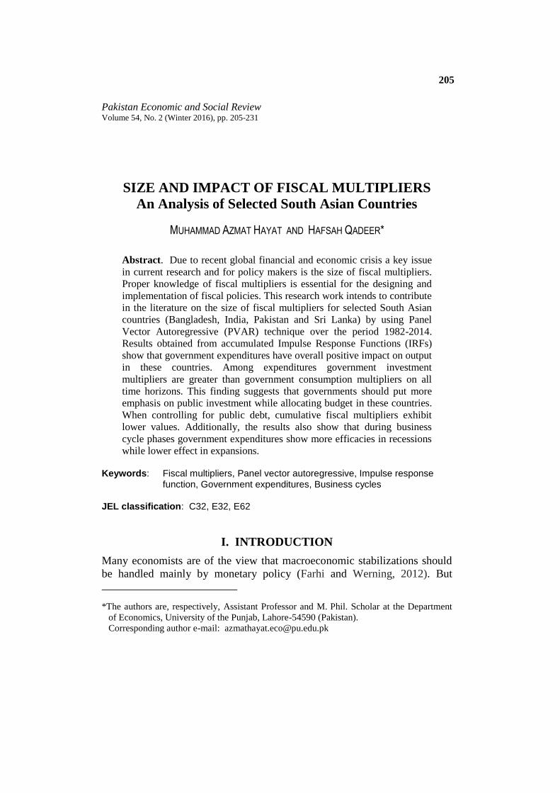
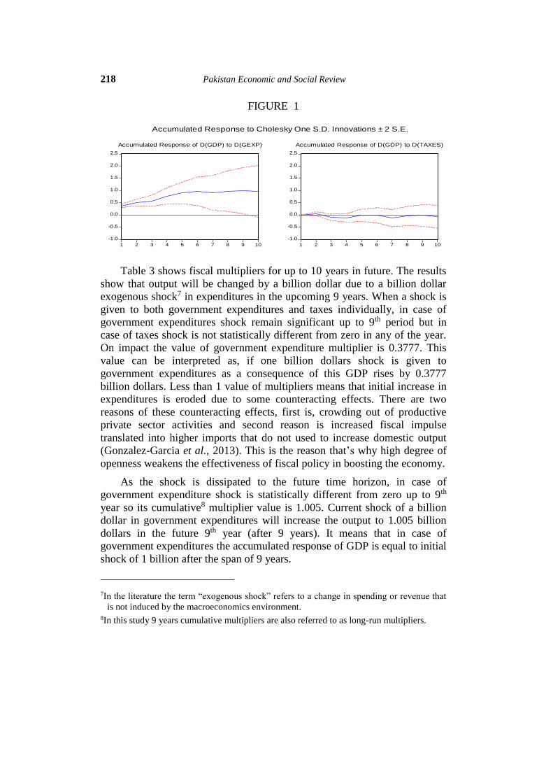
exogenous variable. Figure 1 shows the accumulated impulse response
function of D(GDP) to a shock in D(GEXP) and D(TAXES). Accordingly
government expenditures have an overall positive impact on output. Initially
taxes show positive effect but later on it becomes negative. On x-axis
numbers of years are plotted (from 1-10 years in future) and on y-axis value
of the multipliers (change in output due to a shock in the given fiscal
instrument) are plotted.
In Figure 1, Accumulated IRFs of GDP (at first difference) to shock in
Government Expenditures (at first difference) and taxes (at first difference)
respectively, aggregate model. Dotted lines show upper and lower bounds
and smooth line shows behaviour of variable (GDP).
6
VariableFiscalinChangePercentage
OutputinChanePercentageElasticity
Page 14
218 Pakistan Economic and Social Review
FIGURE 1
-1.0
-0.5
0.0
0.5
1.0
1.5
2.0
2.5
1 2 3 4 5 6 7 8 9 10
Accumulated Response of D(GDP) to D(GEXP)
-1.0
-0.5
0.0
0.5
1.0
1.5
2.0
2.5
1 2 3 4 5 6 7 8 9 10
Accumulated Response of D(GDP) to D(TAXES)
Accumulated Response to Cholesky One S.D. Innovations ± 2 S.E.
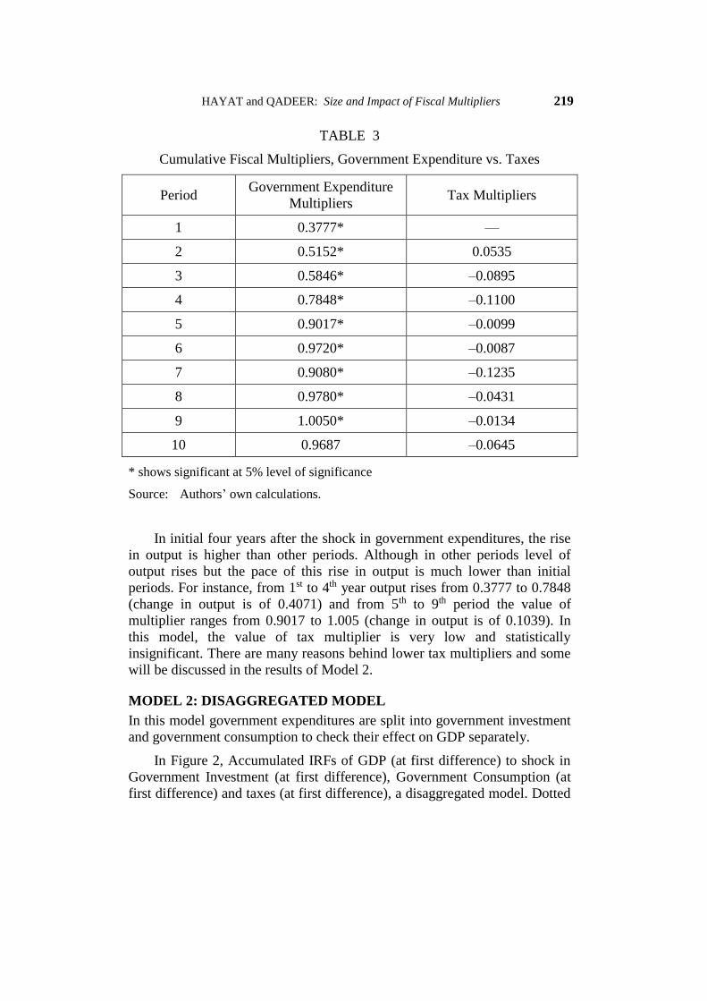
Table 3 shows fiscal multipliers for up to 10 years in future. The results
show that output will be changed by a billion dollar due to a billion dollar
exogenous shock7 in expenditures in the upcoming 9 years. When a shock is
given to both government expenditures and taxes individually, in case of
government expenditures shock remain significant up to 9th period but in
case of taxes shock is not statistically different from zero in any of the year.
On impact the value of government expenditure multiplier is 0.3777. This
value can be interpreted as, if one billion dollars shock is given to
government expenditures as a consequence of this GDP rises by 0.3777
billion dollars. Less than 1 value of multipliers means that initial increase in
expenditures is eroded due to some counteracting effects. There are two
reasons of these counteracting effects, first is, crowding out of productive
private sector activities and second reason is increased fiscal impulse
translated into higher imports that do not used to increase domestic output
(Gonzalez-Garcia et al., 2013). This is the reason that’s why high degree of
openness weakens the effectiveness of fiscal policy in boosting the economy.
As the shock is dissipated to the future time horizon, in case of
government expenditure shock is statistically different from zero up to 9th
year so its cumulative8 multiplier value is 1.005. Current shock of a billion
dollar in government expenditures will increase the output to 1.005 billion
dollars in the future 9th year (after 9 years). It means that in case of
government expenditures the accumulated response of GDP is equal to initial
shock of 1 billion after the span of 9 years.
7In the literature the term “exogenous shock” refers to a change in spending or revenue that
is not induced by the macroeconomics environment. 8In this study 9 years cumulative multipliers are also referred to as long-run multipliers.
Page 15
HAYAT and QADEER: Size and Impact of Fiscal Multipliers 219
TABLE 3
Cumulative Fiscal Multipliers, Government Expenditure vs. Taxes
Period Government Expenditure
Multipliers Tax Multipliers
1 0.3777* —
2 0.5152* 0.0535
3 0.5846* –0.0895
4 0.7848* –0.1100
5 0.9017* –0.0099
6 0.9720* –0.0087
7 0.9080* –0.1235
8 0.9780* –0.0431
9 1.0050* –0.0134
10 0.9687 –0.0645
* shows significant at 5% level of significance
Source: Authors’ own calculations.
In initial four years after the shock in government expenditures, the rise
in output is higher than other periods. Although in other periods level of
output rises but the pace of this rise in output is much lower than initial
periods. For instance, from 1st to 4th year output rises from 0.3777 to 0.7848
(change in output is of 0.4071) and from 5th to 9th period the value of
multiplier ranges from 0.9017 to 1.005 (change in output is of 0.1039). In
this model, the value of tax multiplier is very low and statistically
insignificant. There are many reasons behind lower tax multipliers and some
will be discussed in the results of Model 2.
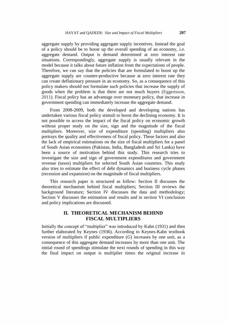
MODEL 2: DISAGGREGATED MODEL
In this model government expenditures are split into government investment
and government consumption to check their effect on GDP separately.
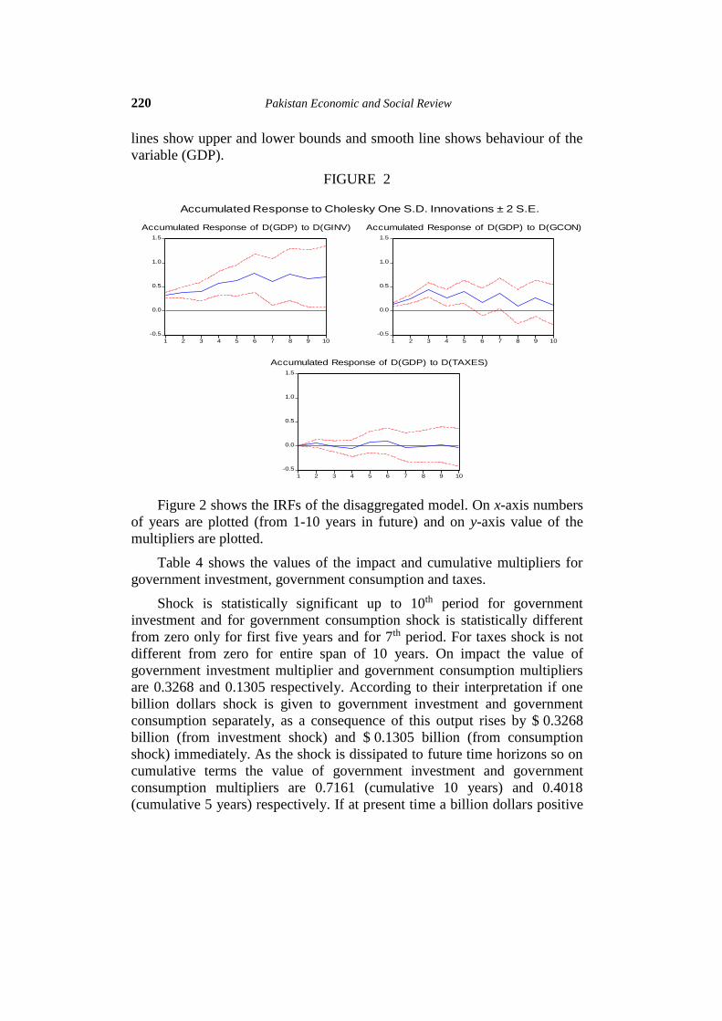
In Figure 2, Accumulated IRFs of GDP (at first difference) to shock in
Government Investment (at first difference), Government Consumption (at
first difference) and taxes (at first difference), a disaggregated model. Dotted
Page 16
220 Pakistan Economic and Social Review
lines show upper and lower bounds and smooth line shows behaviour of the
variable (GDP).
FIGURE 2
-0.5
0.0
0.5
1.0
1.5
1 2 3 4 5 6 7 8 9 10
Accumulated Response of D(GDP) to D(GINV)
-0.5
0.0
0.5
1.0
1.5
1 2 3 4 5 6 7 8 9 10
Accumulated Response of D(GDP) to D(GCON)
-0.5
0.0
0.5
1.0
1.5
1 2 3 4 5 6 7 8 9 10
Accumulated Response of D(GDP) to D(TAXES)
Accumulated Response to Cholesky One S.D. Innovations ± 2 S.E.
Figure 2 shows the IRFs of the disaggregated model. On x-axis numbers
of years are plotted (from 1-10 years in future) and on y-axis value of the
multipliers are plotted.
Table 4 shows the values of the impact and cumulative multipliers for
government investment, government consumption and taxes.
Shock is statistically significant up to 10th period for government
investment and for government consumption shock is statistically different
from zero only for first five years and for 7th period. For taxes shock is not
different from zero for entire span of 10 years. On impact the value of
government investment multiplier and government consumption multipliers
are 0.3268 and 0.1305 respectively. According to their interpretation if one
billion dollars shock is given to government investment and government
consumption separately, as a consequence of this output rises by $ 0.3268
billion (from investment shock) and $ 0.1305 billion (from consumption
shock) immediately. As the shock is dissipated to future time horizons so on
cumulative terms the value of government investment and government
consumption multipliers are 0.7161 (cumulative 10 years) and 0.4018
(cumulative 5 years) respectively. If at present time a billion dollars positive
Page 17
HAYAT and QADEER: Size and Impact of Fiscal Multipliers 221
shock is given as a consequence of this after 10 years government investment
will accumulatively increase output up to $ 0.7161 billion and after 5 years
government consumption accumulatively increase output up to $ 0.4018
billion.
TABLE 4
Cumulative Fiscal Multipliers, Disaggregated Model – Government
Investment, Government Consumption, and Taxes
Period
Government
Investment
Multipliers
Government
Consumption
Multipliers
Tax Multipliers
1 0.3268* 0.1305* —
2 0.3847* 0.2519* 0.0550
3 0.4047* 0.4366* –0.0074
4 0.5809* 0.2775* –0.0456
5 0.6359* 0.4018* 0.0814
6 0.7864* 0.1867 0.0999
7 0.6054* 0.3628* –0.0234
8 0.7634* 0.0934 –0.0099
9 0.6741* 0.2630 0.0316
10 0.7161* 0.1265 –0.0259
*shows significant at 5% level of significance
Source: Author’s own calculations.
In short-run9 the effect on an output due to shock in government
investment is lower than other periods, i.e. in short-run change in output is
about $ 0.05 billion (from 1st to 2nd year). Output significantly rises in other
periods up to 6th period than start declining. For instance, the change in
output from 3rd to 6th period is $ 0.38 billion and from 7th to 10th period is
$ 0.11 billion.
9Short-run is defined as a time gap ranging from simultaneous effects to one year distance
from the fiscal shock (Boussard et al., 2013). In this study 1st year is considered as impact
multiplier and up to 2nd year is considered as short-run multipliers.
Page 18
222 Pakistan Economic and Social Review
In case of government consumption multipliers the pace of the rise of
GDP due to shock in government consumption is very slow and less than
government investment multipliers. For instance, in short-run (0.25 vs 0.38)
and in long-run (0.40 vs 0.63). The results indicate that at all time horizons
government consumption multiplier is less than government investment
multipliers. This suggests that during allocation of budget, policy makers
should emphasis on public investment either in the form of infrastructure or
human resource development because it not only have a positive impact on
output at the time of implementation of these measures but also in longer run
it contributes more in output as compared to public consumption.
According to an economic theory, an increase in the output (GDP) can
be attained by increasing the government expenditures. Results of both
aggregate and disaggregated models of this study support this fact. On the
other hand, according to fiscal multiplier literature the value of government
investment multiplier is higher than government consumption multipliers.
This fact is also evidenced at all-time horizons, like on impact (0.32 vs 0.13)
and cumulative multipliers are (0.63 vs 0.40).10 In above both models, tax
multipliers are very small and shock in taxes is statistically insignificant.
There might be many reasons behind lower and insignificant tax multipliers
for these countries. Firstly, developing countries usually have lower tax
bases. Typically tax collection is very low in low income countries around
10-20 percent of their GDP, while high income countries collect more taxes
like 40 percent of their GDP (Besley and Persson, 2014). Secondly, low
income countries mostly have many small scale firms and large informal
sector. It is difficult to impose proper taxes on large informal and small
sector of the poor economies, such as village shops and street vendors,
because there is no formal record of their incomes and transactions (Besley
and Persson, 2014). The size of the informal sector is strongly negatively
related to income taxation (Schneider, 2002). Thirdly, these countries have
agrarian economies in which farmer’s incomes are seasonal and unstable, so
it’s difficult to calculate base for an income tax. Therefore, taxes play a
diminishing role in these economies (Tanzi and Zee, 2001). Fourthly,
governments of developing countries have alternative sources for revenues
such as foreign aid, which are sometime larger than domestically generated
tax revenues and a significant fraction of GDP. For example, according to
World Development Indicators (WDI) for a sample of low income countries
the average share of aid was around 10 percent of their gross national income
10In case of government consumption multipliers shock is significant accumulatively and
consecutively up to 5th period that is why both multipliers are compared for 5th period.
Page 19
HAYAT and QADEER: Size and Impact of Fiscal Multipliers 223
from 1962-2006 (Besley and Persson, 2014). Fifthly, income is unevenly
distributed in developing countries and there was a lack of efficient, well
trained and well educated tax administration (Tanzi and Zee, 2001). These
are the few reasons behind lower and insignificant tax multipliers for these
countries.
All the models show smaller and less than unity values of multipliers.
There may be three possible reasons for the lower value of multipliers in a
panel of these countries. Firstly, usually people of South Asian economies
are habitual of savings like for their future and for some other precautionary
motives but not for investment purposes and savings act as a leakage. The
whole process of multipliers relies on consumptions, as the consumption of
one person is the income of other and so on. But savings act as a leakage,
higher the value of saving lower will be the consumption which gives lower
value of multipliers. Multiplier formula, k = 1/mps, also shows inverse
relation between marginal propensity to save and multiplier. Secondly, it
might be possible that people have more inclinations towards imports which
reduce the value of multipliers as imports are also leakages in the economy.
Thirdly, greater than unity value of multipliers could be attained when
interest rate is at its lower bound. Unlike developed nations, South Asian
economies do not face the situation of lower bound on interest rate.
MODEL 3: ROLE OF DEBT
In this era of rapid growth and development it is very difficult for a nation to
finance its all development expenditures with its own resources. Therefore to
cover the gap between revenue and expenditures it has to borrow from some
external and internal sources. As far as the contribution of the debt is
concerned, approximately one third effect of debt on growth is through
physical capital accumulation and two third is through the growth in total
factor productivity (Poirson et al., 2004). But as all knows that debt is a
burden and when a nation starts repaying it, it usually increases than its
principal value. Developing nations do not have sufficient capacity to absorb
the external debt positively, as a result, debt exerts negative impact on their
economies. Debt repayments are act as a leakage in the economy so it leads
to lowering the value of the fiscal multipliers.
For assessing the impact of debt dynamics aggregate Panel VAR
(PVAR) model has been re-estimated by just using three variables
(government expenditure, GDP and taxes) as endogenous without controlling
for debt (debt is not considered as exogenous)
Page 20
224 Pakistan Economic and Social Review
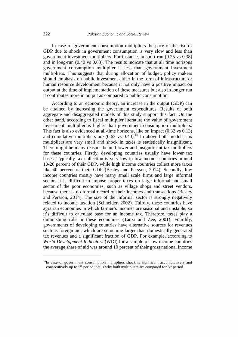
For this model equation (3) is estimated and Table 5 presents the
cumulative value of government expenditure multipliers without controlling
for debt dynamics, and compared the multipliers with aggregate model that is
calculated by controlling (as an exogenous) debt dynamics. All the
multipliers are statistically different from zero for all time horizons and
model is also stable.
TABLE 5
Comparison of Government Expenditure Multipliers with and
without Controlling for Debt Dynamics
Period Government Expenditure Multipliers
without controlling for debt controlling for debt
1 0.3560* 0.3777*
2 0.4693* 0.5152*
3 0.4994* 0.5846*
4 0.6546* 0.7848*
5 0.7259* 0.9017*
6 0.7788* 0.9720*
7 0.8120* 0.9080*
8 0.9046* 0.9780*
9 0.9811* 1.0050*
10 0.9853* 0.9687
* shows significant at 5% level of significance.
Source: Authors’ own calculations.
Table 5 shows that, on impact the value of government expenditure
multiplier is 0.3560 without controlling for debt which is lower than
controlled model (i.e. 0.3777). This model shows that at all time horizons the
value of government expenditure multipliers are less than as compared to
controlled model. These results are consistent with many studies that show
that debt burden hinders the economic growth of a country (Ilzetzki et al.,
2013; Batini et al., 2014; Calderon and Fuentes, 2013).
Page 21
HAYAT and QADEER: Size and Impact of Fiscal Multipliers 225
The short-run period shows that if government expenditures are
increased by a billion dollar it leads to increase the output by 0.11 billion
dollars, which is less than controlled model because debt acts as a leakage in
the economy. Same is the case with long-run multiplier as its value is 0.9811
(which is lower than 1.005 in a controlled model).
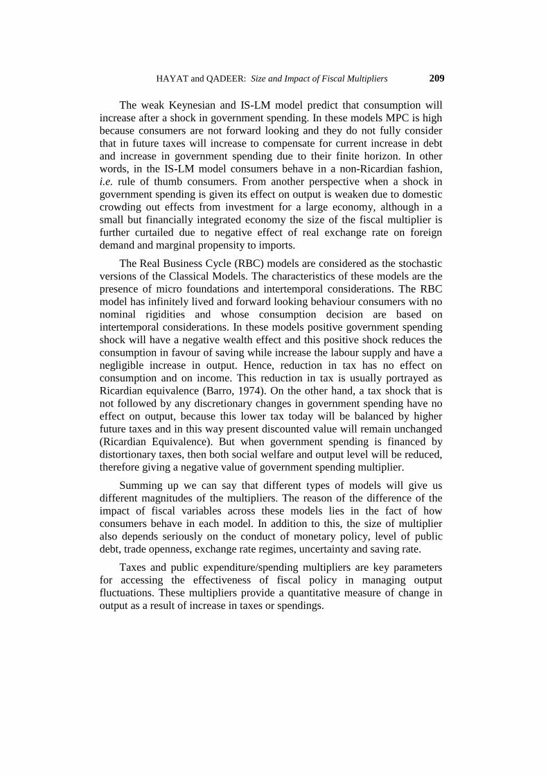
MODEL 4: FISCAL MULTIPLIERS ACROSS BUSINESS CYCLE
PHASES
Baseline (aggregate) PVAR model is re-estimated for analyzing multipliers
across business cycle phases. GDP series is detrended with the help of
Hodrick-Prescott (HP filter) technique to compute output gaps. According to
this two samples are obtained: one sub-sample includes observations that
have positive output gap (expansions) and the other sub-sample contains
observations having negative output gap (recessions). In this case sample
size is reduced therefore appropriate lag length is 1.
FIGURE 3
-2
-1
0
1
2
1 2 3 4 5 6 7 8 9 10
Accumulated Response of D(GDP) to D(GEXP)
Accumulated Response to Cholesky One S.D. Innovations ± 2 S.E.
In Figure 3, Accumulated impulse response function of GDP (at first
difference) due to shock in Government Expenditures (at first difference), in
expansions. Dotted lines show upper and lower bounds and smooth line
shows behaviour of variable.
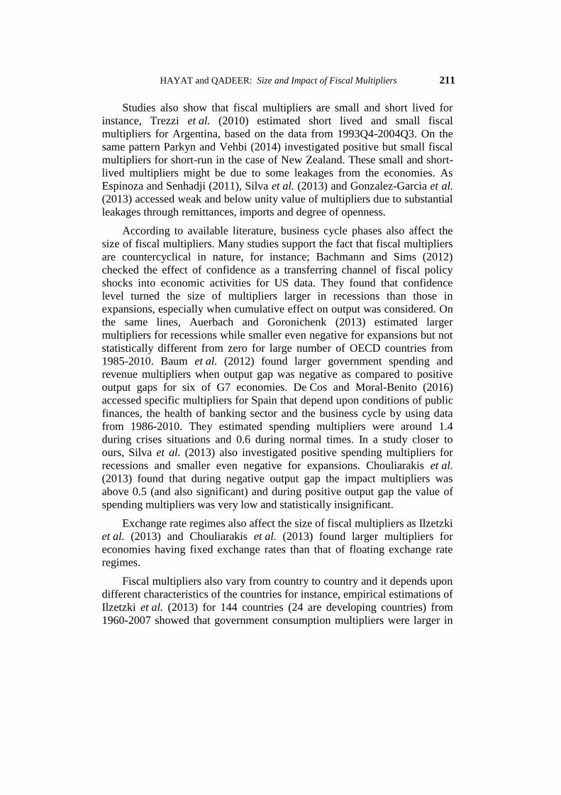
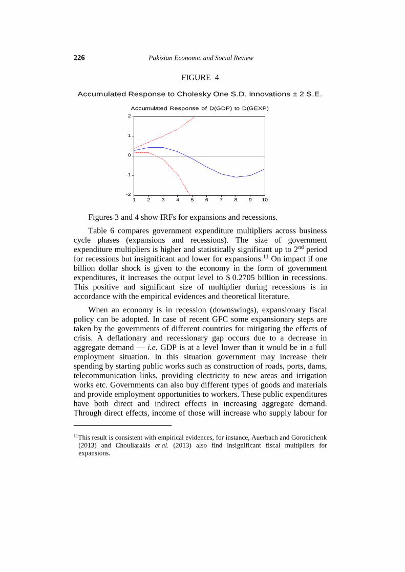
In Figure 4, Accumulated impulse response function of GDP (at first
difference) due to shock in Government Expenditures (at first difference), in
recessions. Dotted lines show upper and lower bounds and smooth line
shows behaviour of variable.
Page 22
226 Pakistan Economic and Social Review
FIGURE 4
-2
-1
0
1
2
1 2 3 4 5 6 7 8 9 10
Accumulated Response of D(GDP) to D(GEXP)
Accumulated Response to Cholesky One S.D. Innovations ± 2 S.E.
Figures 3 and 4 show IRFs for expansions and recessions.
Table 6 compares government expenditure multipliers across business
cycle phases (expansions and recessions). The size of government
expenditure multipliers is higher and statistically significant up to 2nd period
for recessions but insignificant and lower for expansions.11 On impact if one
billion dollar shock is given to the economy in the form of government
expenditures, it increases the output level to $ 0.2705 billion in recessions.
This positive and significant size of multiplier during recessions is in
accordance with the empirical evidences and theoretical literature.
When an economy is in recession (downswings), expansionary fiscal
policy can be adopted. In case of recent GFC some expansionary steps are
taken by the governments of different countries for mitigating the effects of
crisis. A deflationary and recessionary gap occurs due to a decrease in
aggregate demand — i.e. GDP is at a level lower than it would be in a full
employment situation. In this situation government may increase their
spending by starting public works such as construction of roads, ports, dams,
telecommunication links, providing electricity to new areas and irrigation
works etc. Governments can also buy different types of goods and materials
and provide employment opportunities to workers. These public expenditures
have both direct and indirect effects in increasing aggregate demand.
Through direct effects, income of those will increase who supply labour for
11This result is consistent with empirical evidences, for instance, Auerbach and Goronichenk
(2013) and Chouliarakis et al. (2013) also find insignificant fiscal multipliers for
expansions.
Page 23
HAYAT and QADEER: Size and Impact of Fiscal Multipliers 227
these projects and sell materials. The output of these public works also goes
up together with the increase in incomes. As the consumption of one person
is the income of other therefore, who gets more income they spend further on
consumer goods according to their MPC. This thing creates multiplier
effects. Another tool of expansionary fiscal policy is to cut taxes, which will
have an indirect effect on aggregate demand curve by increasing the
disposable income of the consumers.
TABLE 6
Government Expenditure Multipliers for Expansions and Recessions
Period Government Expenditure Multipliers
Recessions Expansions
1 0.2705* 0.0144
2 0.4335* 0.0455
* shows significant at 5% level of significance
Source: Authors’ own calculations.
Another important argument is that the simplest Keynesian model also
assumes excess capacities in the economy. As during the periods of
recessionary gaps there exist some excess capacities in the consumer goods
industries, therefore, expansionary public spending promote optimism in the
“animal spirits” of the entrepreneurs. Once the expectations of the
entrepreneurs will become optimistic, they will make use of idle capacity,
demanding larger workforce and eventually more investment and so expand
their productive capacity and these excess capacities also lowers the
probability of crowding out of private investment. In short positive climate
will increase effective demand and with it employment, consumption and
revenues initialing cumulative, virtuous circle of growth. Due to these excess
capacities expansionary fiscal policy will yield higher value of government
expenditure multipliers in recession than in expansions.
VI. CONCLUSIONS
Size of the fiscal multipliers is always a great scrutiny for both policy makers
and economists because multipliers are among one of many factors that need
to be considered in setting fiscal policy. In this context, this research work
intends to contribute the literature on the size and magnitude of the fiscal
multipliers for selected South Asian economies (Bangladesh, India, Pakistan
Page 24
228 Pakistan Economic and Social Review
and Sri Lanka) by using Panel VAR model relying on annual time span from
1982-2014.
Estimated results shows that for baseline (aggregate) model government
expenditures have overall positive impact on output. Among the
expenditures government investment is the main driving force for increasing
output and government investment multiplier is greater than government
consumption multipliers on all time horizons. During allocation of budget
policy makers should put more emphasis on public investment either in the
form of infrastructure or human resource development because it not only
has a positive impact on output at the time of implementation of these
measures but in long-run also.
Debt is always a burden for lower middle income countries and debt
servicing act as leakages in the economy. As a consequence of this when
aggregate model is re-estimated without controlling for debt dynamics, it
gives impact and cumulative (long-run) multipliers lower than that of
controlled model. Additionally, this research supports that across business
cycle phases the efficiency and effectiveness of government expenditures is
larger in recessions and lower in expansions. The size of government
expenditure multiplier is higher in recessions as compared to expansions.
According to the results of this research, the concerned authorities of
these countries should give more emphasis on government investment
expenditures, especially in the field of skill development and capital
accumulation as these are helpful in enhancing the productivity of a nation.
Page 25
HAYAT and QADEER: Size and Impact of Fiscal Multipliers 229
REFERENCES
Auerbach, A. J. and Y. Gorodnichenko (2013), Fiscal multipliers in recession and
expansion. In Alesina and Giavazzi, Fiscal Policy after the Financial Crisis.
University of Chicago Press.
Bachmann, R. and E. R. Sims (2012), Confidence and the transmission of
government spending shocks. Journal of Monetary Economics, Volume 59(3),
pp. 235-249. http://dx.doi.org/10.1016/j.jmoneco.2012.02.005
Barro, R. J. (1974), Are government bonds net wealth? Journal of Political
Economy, Volume 82(6), pp. 1095-1117. http://dx.doi.org/10.1086/260266
Batini, N., Eyraud, L., and Weber, A. (2014). A Simple Method to Compute Fiscal
Multipliers (No. 14-93). International Monetary Fund.
Baum, A., M. Poplawski-Ribeiro and A. Weber (2012), Fiscal multipliers and the
state of the economy. IMF Working Paper # 12/286.
Besley, T. and T. Persson (2014), Why do developing countries tax so little?
Journal of Economic Perspectives, Volume 28(4), pp. 99-120.
http://dx.doi.org/10.1257/jep.28.4.99
Blanchard, O. and R. Perotti (1999), An empirical characterization of the dynamic
effects of changes in government spending and taxes on output. NBER
Working Paper # 7269.
Bose, S. and N. R. Bhanumurthy (2015), Fiscal Multipliers for India. Margin: The
Journal of Applied Economic Research, Volume 9(4), pp. 379-401.
http://dx.doi.org/10.1177/0973801015598585
Boussard, J., F. De Castro and M. Salto (2013), Fiscal Multipliers and Public Debt
Dynamics in Consolidations. Springer, Milan.
Calderón, C., and Fuentes, J. R. (2013). Government Debt and Economic
Growth. IDB Working Paper Series IDB-WP-424.
Choi, I. (2001), Unit root tests for panel data. Journal of International Money and
Finance, Volume 20(2), pp. 249-272.
http://dx.doi.org/10.1016/S0261-5606(00)00048-6
Chouliarakis, G., T. Gwiazdowski and S. Lazaretou (2013), Fiscal Multipliers in
Times of Crises and Prosperity: Historical Evidence from Greece. Bank of
Greece.
Christiano, L., M. Eichenbaum and S. Rebelo (2011), When is the government
spending multiplier large? Journal of Political Economy, Volume 119(1), pp.
78-121. http://dx.doi.org/10.1086/659312
Page 26
230 Pakistan Economic and Social Review
De Cos, P. H. and E. Moral-Benito (2016), Fiscal multipliers in turbulent times: The
case of Spain. Empirical Economics, Volume 50(4), pp. 1589-1625.
http://dx.doi.org/10.1007/s00181-015-0969-0
Eggertsson, G. B. (2011), What fiscal policy is effective at zero interest rates?
In NBER Macroeconomics Annual 2010, University of Chicago Press.
Espinoza, R. A. and A. S. Senhadji (2011), How strong are fiscal multipliers in the
GCC? An empirical investigation. IMF Working Paper # 11/61.
Farhi, E. and I. Werning (2012), Fiscal multipliers: Liquidity traps and currency
unions. NBER Working Paper # 18381. http://dx.doi.org/10.3386/w18381
Gonzalez-Garcia, J., A. Lemus and M. Mrkaic (2013), Fiscal Multipliers in the
ECCU. IMF Working Paper # 13/117.
Ilzetzki, E., E. G. Mendoza and C. A. Végh (2013), How big (small?) are fiscal
multipliers? Journal of Monetary Economics, Volume 60(2), pp. 239-254.
http://dx.doi.org/10.1016/j.jmoneco.2012.10.011
Im, K. S., M. H. Pesaran and Y. Shin (2003), Testing for unit roots in heterogeneous
panels. Journal of Econometrics, Volume 115(1), pp. 53-74.
http://dx.doi.org/10.1016/S0304-4076(03)00092-7
Jemec, N., Kastelec, A. S., and Delakorda, A. (2011): How do fiscal shocks affect
the macroeconomic dynamics in the Slovenian economy. Prikazi in analize
2/2011, Banka Slovenije.
Kahn, R. F. (1931). The Relation of Home Investment to Unemployment. The
Economic Journal. Wyley-Blackwell. 41 (162).
https://dx.doi.org/10.2307%2F2223697
Keynes, J. M. (1936). The general theory of interest, employment and
money. London: Macmillan
Love, I. and L. Zicchino (2006), Financial development and dynamic investment
behavior: Evidence from panel VAR. Quarterly Review of Economics and
Finance, Volume 46(2), pp. 190-210.
http://dx.doi.org/10.1016/j.qref.2005.11.007
Lütkepohl, H. (2011), New Introduction to Multiple Time Series Analysis.
Springer-Verlag Berlin Heidelberg.
http://dx.doi.org/10.1007/978-3-540-27752-1
Maddala, G. S. and S. Wu (1999), A comparative study of unit root tests with panel
data and a new simple test. Oxford Bulletin of Economics and Statistics,
Volume 61(S1), pp. 631-652. http://dx.doi.org/10.1111/1468-0084.0610s1631
Marattin, L. and S. Salotti (2011), On the usefulness of government spending in the
EU area. The Journal of Socio-Economics, Volume 40(6), pp. 780-795.
http://dx.doi.org/10.1016/j.socec.2011.08.018
Page 27
HAYAT and QADEER: Size and Impact of Fiscal Multipliers 231
Marattin, L., and Salotti, S. (2011). On the usefulness of government spending in
the EU area. The Journal of Socio-Economics, 40(6), 780-795.
Minea, A. and L. Mustea (2015), A fresh look at fiscal multipliers: one size fits it
all? Evidence from the Mediterranean area. Applied Economics, Volume
47(26), pp. 2728-2744. http://dx.doi.org/10.1080/00036846.2015.1008775
Owyang, M. T., V. A. Ramey and S. Zubairy (2013), Are government spending
multipliers greater during periods of slack? Evidence from twentieth-century
historical data. The American Economic Review, Volume 103(3), pp. 129-134.
http://dx.doi.org/10.1257/aer.103.3.129
Parkyn, O. and T. Vehbi (2014), The effects of fiscal policy in New Zealand:
Evidence from a VAR model with debt constraints. Economic Record, Volume
90(290), pp. 345-364. http://dx.doi.org/10.1111/1475-4932.12116
Poirson, H., L. A. Ricci and C. A. Pattillo (2004), What are the channels through
which external debt affects growth? IMF Working Paper # 04/15.
Schneider, F. (2002), Size and measurement of the informal economy in 110
countries around the world. In Workshop of Australian National Tax Centre,
ANU, Canberra.
Silva, R., V. M. Carvalho and A. P. Ribeiro (2013), How large are fiscal
multipliers? A panel-data VAR approach for the Euro area. FEP Working
Paper # 500, Faculty of Economics, University of Porto.
Sims, C. A. (1980), Macroeconomics and reality. Econometrica, Volume 48(1), pp.
1-48. http://dx.doi.org/10.2307/1912017
Tanzi, V. and H. H. Zee (2001), Tax policy for developing countries. Economic
Issues # 27. International Monetary Fund.
Trezzi, R., P. Anos-Casero and D. Cerdeiro (2010), Estimating the fiscal multiplier
in Argentina. World Bank Policy Research Working Paper # 5220.
http://dx.doi.org/10.1596/1813-9450-5220
Yadav, S., V. Upadhyay, S. Sharma (2012), Impact of fiscal policy shocks on the
Indian economy. Margin: Journal of Applied Economic Research, Volume
6(4), pp. 415-444. http://dx.doi.org/10.1177/0973801012462171