1 The AeioTu Early Childhood Longitudinal Study Report I. Baseline Data Collection National Institute for Early Education Research and Universidad de los Andes-CEDE Please do not cite without permission Last update, February 2012 Introduction In collaboration with aeioTU, NIEER is conducting a randomized trial comparing the effects of aeioTU's early childhood development (ECD) intervention in 2 aeioTU centers in Santa Marta, Colombia. The study design was formulated to investigate individual child growth and development in social, health, cognitive, and emotional area. The design also allows to accurately estimate the effects of the aeioTU preschool experience on children´s cognitive and non-cognitive outcomes and at primary school entry. Moreover, it will allow the research team to study the costs and benefits of the aeioTU program for individuals and society. The aim of this progress report is to describe baseline data collected from mid-2010 to early-2011. Baseline collection was funded in a 62% by the Jacobs Foundation, 16% by Fundación Carulla and 22% by the IADB. Summary Two communities in the city of Santa Marta were included in our study: Timayui and La Paz. Baseline data collection was carried out in both communities. A total 1,219 children were assessed in both communities from mid-July 2010 to early-January 2011. In November 2010 and February 2011, sampled children in Timayui and La Paz respectively participated in lotteries intended to assign school slots. In Table 1 we show baseline sample size by community, by child’s age and by intent to treat status. Table 1. Baseline sample size by age, by community and by intent to treat status Age group Timayui La Paz Total Lottery winners Lottery losers Lottery winners Lottery losers Lottery winners Lottery losers <1 38 75 30 24 68 99 1-2 63 80 56 96 119 176 2-3 82 61 56 123 138 184 3-4 57 45 64 97 121 142 4-5 29 14 69 60 98 74 Total 269 275 275 400 544 675 In particular, we show total sample size by community split by lottery status: winners and losers. As can be observed, total treatment group is 544 out of 1,219 total sample
Transcript
1
The AeioTu Early Childhood Longitudinal Study Report I. Baseline Data Collection
National Institute for Early Education Research and Universidad de los Andes-CEDE
Please do not cite without permission
Last update, February 2012
Introduction In collaboration with aeioTU, NIEER is conducting a randomized trial comparing the effects of aeioTU's early childhood development (ECD) intervention in 2 aeioTU centers in Santa Marta, Colombia. The study design was formulated to investigate individual child growth and development in social, health, cognitive, and emotional area. The design also allows to accurately estimate the effects of the aeioTU preschool experience on children´s cognitive and non-cognitive outcomes and at primary school entry. Moreover, it will allow the research team to study the costs and benefits of the aeioTU program for individuals and society. The aim of this progress report is to describe baseline data collected from mid-2010 to early-2011. Baseline collection was funded in a 62% by the Jacobs Foundation, 16% by Fundación Carulla and 22% by the IADB. Summary Two communities in the city of Santa Marta were included in our study: Timayui and La Paz. Baseline data collection was carried out in both communities. A total 1,219 children were assessed in both communities from mid-July 2010 to early-January 2011. In November 2010 and February 2011, sampled children in Timayui and La Paz respectively participated in lotteries intended to assign school slots. In Table 1 we show baseline sample size by community, by child’s age and by intent to treat status.
Table 1. Baseline sample size by age, by community and by intent to treat status
In particular, we show total sample size by community split by lottery status: winners and losers. As can be observed, total treatment group is 544 out of 1,219 total sample
2
size and the control group is 675. There are some differences by community. In particular, in Timayui, the split is roughly half and half between lottery winners and lottery losers out of a total 544 children assessed in baseline. In La Paz, 40% correspond to winners and the remainder 60% corresponds to lottery losers out of a total 675 children assessed in baseline. The distribution also varies somewhat by age. In particular, the fraction of lottery winners goes from 40% at less than one year of age to 56% at 4 to 5 years of age always monotonically increasing as a fraction of total number of assessed children by age range. This is due to the distribution of ages at the centers, with a very small number of slots available for younger children a larger number for older children. With these sample sizes we expect to be able to estimate cohort/intensity effects at least splitting the sample into younger than 2 and older than 2. In Table 2 we summarize the list of instruments that were collected by child’s age. The cookie test was only collected in Timayui due to implementation problems and small sample sizes. In addition, we collected a comprehensive household survey of all parents in our sample, including characteristics of the household, characteristics of adult members of the household, characteristics of other children in the household, the child’s child care history, among others. Table 2. List of instruments by child’s age CHILDREN 0-3 YEARS OF AGE CHILDREN 3-5 YEARS OF AGE
(Squires et al. 1999) 5) Self-regulation HTKS (Head, Toes, Knees and Shoulders)
6) Socio-emotional Ages & Stages Questionnaire
7) Delayed gratification "cookie test"
Baseline Data Description: Household Sociodemographic Characteristics In this report we present a basic baseline data description by intent to treat status. In the tables to follow, the treatment group is understood as the group of lottery winners (intended to be treated) and the control group is understood as the group of lottery losers. We start by showing characteristics of the household and the family by intent to treat status. The last two columns in each case show the relevant statistic and its p-value to assess mean or distribution difference between the two groups. Lack of stars in the p-value indicates that both groups are statistically identical in that dimension.
3
We start by showing in Table 3 characteristics of the household, availability of public utilities and other characteristics of the family. In panel A we show the type of house where the child’s family resides, the type of walls and floor. Most of the families in the sample (around 70%) leave in a house rather than an apartment or a room, which is quite typical in the Atlantic region in Colombia. Most of these houses are characterized by bricked / blocked walls and cement / gravel floors. There are no statistically significant differences between the two groups by these items. Table 3. Characteristics of the household
A. House conditions
All Treate
d Controle
d
Pearson
Chi2
P value
Type of House 1199 534 665 5.97 0.11
House 70.1% 68.5% 71.3%
Apartment 7.8% 6.6% 8.9% Room(s) in a house or apartment 4.3% 5.1% 3.6% Another type of shelter 17.8% 19.9% 16.2% Exterior walls 1200 536 664 3.48 0.84
Carpet, marble, parquet, polished wood or lacquered 2.1% 2.1% 2.1%
Tile, vinyl, tablet, brick 7.3% 5.8% 8.5%
Cement, gravel 80.0% 80.6% 79.5%
Crude wooden, planks, another plant 0.1% 0.2% 0.0%
Dirt, sand 10.3% 11.2% 9.6%
Other 0.2% 0.2% 0.1% * Significant at 10% level, ** at 5% level, *** at 1% level
4
In panel B we show characteristics of the bathroom and availability of some basic public utilities. Most of the households in the sample have a toilet connected to septic tank and less than 31% are connected to sewer, which reveals that both communities are quite poor. Some 2% to 4% do not have a bathroom in their house. Most households also have their own bathroom for exclusive use of the member of the household. However, close to 6% to 8% either do not have a bathroom or have to share with other families. Finally, in most households the bathroom is located inside the house (close to 55%) while close to 35% have a bathroom but outside the house within their property. Only the type of bathroom connection seems to be statistically different between the two groups being the treatment group more likely to be connected to sewer. Table 3. Characteristics of the household (continuation)
A. Bathroom
All Treat
ed Contro
ls
Pearson
Chi2
P value
Bathroom service 1206 537 669 10.3
7 0.04 **
Toilet connected to sewer 27.4% 31.1% 24.5%
Toilet connected to septic tank 69.0% 64.6% 72.5% Toilet with no connection, latrine 0.3% 0.2% 0.4% Other 0.2% 0.4% 0.1% They do not have a bathroom 3.0% 3.7% 2.4% Bathroom Use 1191 528 663 4.27 0.12
Exclusively by the people who reside in 92.4% 91.5% 93.2%
In a sharing arrangement with people from other homes 4.5% 4.4% 4.7%
They do not have a bathroom 3.0% 4.2% 2.1% Water supply: Location of the key, tap or well 1199 533 666 8.05
0.09 *
Inside the house 55.8% 56.7% 55.1%
Outside the house but within the lot or property 36.4% 34.5% 37.8%
Outside of the house and the lot or property 3.3% 2.8% 3.8%
Other 4.4% 6.0% 3.2% * Significant at 10% level, ** at 5% level, *** at 1% level
Finally, panel C shows the use of other public utilities including water, electricity and gas. As can be observed, 40% to 50% receive clean water at home through public aqueduct; while close to 30% have access to clean water through a public fountain. Something close to 18% has access through a communal aqueduct. There seems to be a
5
significant difference between treatment and control groups with the control group reporting better access to clean water through public aqueduct at their own homes. Close to half the families have a separate kitchen for cooking at home, while 28% report having a kitchen within their living room and 14% cooking in a room that is also used to sleep. Finally, only about 13% households report they cook with electricity while 30% to 40% of households cook with natural gas through public pipeline. A large fraction of households, close to 50%, cook with gas cylinder or pipette. In this case, also the control group seems to have better access to clean water and safer ways of cooking that the treatment group. In Table 4 we show the fraction of households that had been previously displaced by the social conflict in Colombia, and the reasons for displacement. In particular, we observe that close to 35% of households have actually been displaced (and arrived to one of our communities as a consequence) as a result of the social conflict in the country. Close to 65% of these, report that the actor of social conflict responsible for their displacement was the guerilla. In a smaller proportion, they also report paramilitaries, government and other types of armed conflict. Table 3. Characteristics of the household (continuation)
A. Food preparation All
Treated
Controled
Pearson Chi2
P value
Water for drinking or food preparation 1203 537 666 26.51 0.002 *** Public aqueduct 45.1% 39.1% 50.0%
Communal aqueduct 18.2% 17.9% 18.5% Public fountain 25.4% 30.2% 21.6% Well with a pump 0.7% 1.1% 0.3% Well without a pump 0.1% 0.0% 0.2% River, creek, spring 0.3% 0.4% 0.3% Water truck or water boy 0.7% 1.3% 0.3% Bottled water or bag 5.8% 5.8% 5.9% Rainwater 0.1% 0.2% 0.0% Other 3.5% 4.1% 3.0% Where are meals prepared in your home 1198 535 663 3.72 0.59 In a room used for cooking 53.8% 53.3% 54.1%
In room that is also used to sleep 14.0% 13.5% 14.5%
In a living or dining room 28.4% 29.3% 27.6%
In a courtyard, corridor, arbor or outdoors 2.3% 1.9% 2.7%
Meals are not prepared at home 1.2% 1.7% 0.8%
Other 0.3% 0.4% 0.3% Fuel or energy used to cook in your home 1189 528 661 20.83 0.002 ***
6
Electricy 13.5% 13.6% 13.3%
Natural gas connected to a public line 35.8% 30.3% 40.2%
Gas cylinder or pipette 45.6% 48.9% 43.0%
Oil, gasoline, kerosene, alcohol 0.3% 0.4% 0.2%
Wood, waste materials, charcoal 3.9% 5.1% 2.9%
Coal 0.7% 1.3% 0.2%
Other 0.3% 0.4% 0.3% * Significant at 10% level, ** at 5% level, *** at 1% level
Table 4. Forced displacement
Displacement All
Treated
Controled
Pearson Chi2
P value
Been displaced from home due to violence 1191 528 663 1.14
0.57
No 66.0% 65.2% 66.7% Yes 33.9% 34.8% 33.2%
Guerilla 309 147 162 4.21 0.04
**
No 62.8% 68.7% 57.4% Yes 37.2% 31.3% 42.6%
Paramilitary 345 163 182 0.78 0.38
No 48.4% 50.9% 46.2% Yes 51.6% 49.1% 53.8%
Government 271 132 139 1.06 0.30
No 99.6% 99.2% 100.0% Yes 0.4% 0.8% 0.0%
Assassination 275 135 140 0.04 0.85
No 94.5% 94.8% 94.3% Yes 5.5% 5.2% 5.7% Kidnappings or torture 270 131 139
Yes 13.5% 10.3% 16.4% * Significant at 10% level, ** at 5% level, *** at 1% level In Table 5 we present a variety of measures of household poverty including public utilities, access to durable goods, SISBEN level and average income / expenses. SISBEN identifies the poorest and most disadvantaged households, families or individuals, for targeting process and unifying social policies. Table 5. Socioeconomic conditions of households
SISBEN All N
Treated Controlled t stat P value
Mean n Mean n
Score 6.69 175 6.52 88 6.87 87 -0.35 0.73
(6.78) (5.37) (7.98)
SISBEN LEVEL All Treated Controls Pearson
Chi2 P value
Level 955 438 517 0.82 0.665 level zero 0.50% 0.70% 0.40% level one 96.60% 96.10% 97.10% level two 2.80% 3.20% 2.50%
* Significant at 10% level, ** at 5% level, *** at 1% level Standard deviation in parentheses
* Significant at 10% level, ** at 5% level, *** at 1% level Households in both groups seem to be very similar in terms of socioeconomic conditions. These households are very poor with SISBEN scores close to 6 (and SISBEN level 1). In terms of access to public utilities, there seem to be some differences between groups but not in a single direction. For example, the treatment group seems to have significantly more access to sewage than the control group but the opposite happens with access to clean water through public aqueduct. With the exception of electricity (almost 100%) and garbage collection (close to 78%), access to other utilities does not surpass 50% in all other cases. There seem to be marginally significant differences in favor of the control groups in terms of ownership of electric shower, TV and computer. Apart from that, no differences emerge in terms of refrigerator, washing machine, blender, electric stove or oven, radio, microwave, etc. Households commonly use a bike as a means of transportation, while about 20% report owning a motorbike. Only 1% of households report owning a car as a means of transportation. No significant differences emerge between groups. Households report owning more than one cellular phone per family.
11
Finally, the distribution of earnings seems similar in both groups, with an average of about 550.000COP or US$300 monthly earnings. In terms of reported total family monthly expenses, the control group reports a slightly higher (but significantly so) amount with an average US$250 compared to US$216 in the treatment group.
Table 6 presents characteristics of mothers of children in our sample. Mothers have on average 8 years of education, with no significant differences between the treatment and control group. Most mothers (close to 60%) are not legally married but rather have cohabitated with their partner for over two years. Only about 9% are legally married and 24% report to be single mothers. Close to 98% of mothers of children in our sample are reported to not live in the household with the child. Only about 23% report to be employed, while close to 70% report they run some kind of business at home (informal employment of some sort). In addition, out of women reporting to be working, 70% are unpaid family workers (also considered as informal employment). All in all, female labor participation is quite low in our sample which also resembles quite well the situation in the Atlantic region. In Table 7 we present similar information for fathers of children in our sample. On average, these fathers have lower educational attainment than children’s mothers, with close to 7.2 years of schooling. No significant differences emerge between groups. Similarly, 30% of fathers do not reside with their children at home. Close to 90% of fathers report to be working (during the previous week), with most report self-employment (50%) or worker/employee (45%).
Table 6. Characteristics of the child’s mother
Mother's education All N
Treated Controlled t stat
Mean n Mean n P value
Years of schooling for mother 8.37 1164 8.34 517 8.40 647 -0.33 0.74 (3.26) (3.09) (3.39)
Mother´s current marital status All
Treated
Controlled
Pearson Chi2
P value
Current marital status 1197 531 666 9.31 0.10
*
Married 8.9% 8.1% 9.6%
Divorced 1.1% 1.1% 1.1% Single 24.2% 24.1% 24.3%
12
Widowed 1.2% 0.4% 1.8%
Marriage-like for more than two years 59.1% 62.0% 56.9%
Marriage-like for less than two years 5.4% 4.3% 6.3%
Mother All Treated Controlled Pearson Chi2 P value
Lives in the household 1203 535 668 1.20 0.27 Yes 97.6% 98.1% 97.2% No 2.4% 1.9% 2.8%
Mother´s employment during the last week All
Treated
Controlled
Pearson
Chi2
P value
Receives payment for work 1173 516 657 2.37 0.50 No 77.7% 78.5% 77.2% Yes 22.1% 21.3% 22.7% Employment 1197 532 665 5.66 0.69 Working 23.8% 23.1% 24.4% Did not work but had a job 0.3% 0.4% 0.2%
Looked for work but had a job before 0.6% 0.9% 0.3%
Looked for work but was working 0.1% 0.0% 0.2%
Looked for work for the first time 0.3% 0.2% 0.5%
Studied 4.8% 4.7% 5.0% Trades conducted from home 69.3% 70.1% 68.6%
Was permanently incapacitated for work 0.2% 0.2% 0.2%
He was in another situation 0.7% 0.4% 0.9% Employment type 939 424 515 3.34 0.65 Worker or employee 7.5% 8.0% 7.0% Government employee or worker 0.2% 0.0% 0.4% Self-employed 13.3% 13.0% 13.6% Domestic employee 10.3% 10.6% 10.1% Unpaid family worker 68.8% 68.2% 68.9%
* Significant at 10% level, ** at 5% level, *** at 1% level
13
Table 7. Characteristics of the child’s father
Father's education
All N
Treated Controlled
t stat
Mean n Mean n P
value Years of schooling for father
8.33 1110
8.32 501 8.34 609 -0.08 0.94
(3.43) (3.28) (3.56)
Father's residency All
Treated
Controlled
Pearson Chi2
P value
Lives in the household 1175 520 655 3.26 0.35 Yes 68.2% 67.5% 68.7% No 29.6% 30.8% 28.7%
Deceased 2.1% 1.5% 2.6%
Father’s employment during the last week All
Treated
Controlled
Pearson Chi2
P value
Receives payment for work 1074 495 579 4.48 0.21 No 24.4% 25.7% 23.3% Yes 75.2% 74.1% 76.2% Employment 1092 498 594 12.04 0.21 Working 88.4% 86.7% 89.7% Did not work but had a job 1.3% 2.0% 0.7%
Looked for work but had a job before 4.9% 5.2% 4.5%
Looked for work but was working 0.5% 0.2% 0.7%
Looked for work for the first time 0.1% 0.2% 0.0%
Studied 0.3% 0.2% 0.3% Trades conducted from home 0.4% 0.4% 0.3%
Was permanently incapacitated for work 0.5% 0.8% 0.3%
He lived by retirement income or rent 0.3% 0.0% 0.5%
He was in another situation 3.5% 4.2% 2.9% Employment type 1000 449 551 2.57 0.77 Worker or employee 44.2% 44.3% 44.1% Government employee or worker 2.1% 2.0% 2.2% Boss or employer 0.3% 0.0% 0.5% Self-employed 52.1% 52.3% 51.9%
* Significant at 10% level, ** at 5% level, *** at 1% level In Table 8 we report information about children’s attendance to childcare. The results indicate that only about 25% of children have actually attended some type of childcare during the last year, with treated children being significantly more likely. From those we have attended over the last year, a vast majority of 88% have used services provided by Instituto Colombiano de Bienestar Familiar (ICBF) such as the widespread program Hogares Comunitarios. There are no significant differences on the type of childcare, on attending any other childcare in the past (beyond just the previous year), or on the type of such care.About 15% of children report that they have attended some sort of childcare in the past (not the last year) and there are no significant differences by group. Almost of all these, report to have used public services provided by ICBF. Table 8. Children’s attendance to childcare
Early childhood experiences All Treated
Controls
Pearson Chi2
P value
Attended childcare last year 1204 536 668 7.48 0.01 ***
No 79.5% 75.9% 82.3% Yes 20.5% 24.1% 17.7% Types of childcare last year 248 125 123
ICBF 88.3% 88.8% 87.8% 1.42 0.70
Private center 9.3% 8.0% 10.6% Relative's home 80.0% 0.8% 0.8% Non-relative's home 1.6% 2.4% 0.8% Attended any other childcare in the past 1178 524 654 1.65
0.20
No 86.0% 84.5% 87.2% Yes 14.0% 15.5% 12.8% Types of other childcare in past 154 77 77 1.23
0.54
ICBF 96.1% 97.4% 94.8% Private center 3.2% 2.6% 3.9% Non-relative's home 0.6% 0.0% 1.3% Other child younger than 10 attend a childcare 821 364 457 6.28
0.01 **
No 83.1% 79.4% 86.0% Yes 16.9% 20.6% 14.0%
Type of childcare center 133 76 57 1.13 0.57
ICBF 82.0% 80.3% 84.2% Private center 14.3% 14.5% 14.0%
15
Non-relative's home 3.8% 5.3% 1.8% * Significant at 10% level, ** at 5% level, *** at 1% level Baseline Data Description: Children’s outcome variables In the tables that follow, we show average outcome variables (following Table 2) by group. We start in Table 9 by showing children’s nutritional status as measured by height, weight and height for weight Z-scores (upper panel) and the corresponding malnutrition measures (lower panel). The results indicate that there are no significant differences in nutritional status by group, but nutritional status is quite poor in our sample. Note that Z-scores for height for age are, on average, one complete standard deviation below what they should be given the child’s gender and age. Weight for age is close to half a standard deviation below and weight for height is barely 0.2 of a standard deviation above average. In all, close to 20% of children in our sample suffer from chronic malnutrition, 4% global malnutrition and 1% acute malnutrition. There are no significant differences by intent to treat status. Table 9. Children’s Nutritional Status
All N
Treated Controls
t test
P value
Mean n Mean n
Length/height-for-age z-score -1.11 1182 -1.1 527 -1.12 655 0.21 0.83 (1.07) (.99) (1.12) Weight-for-age z-score -0.40 1161 -0.46 516 -0.35 645 -1.72 0.09 * (1.03) (.98) (1.06) Weight-for-length/height z-score 0.31 1156 0.25 516 0.35 640 -1.83 0.07 * (0.98) (.95) (1.01) °Z-scores for height for age, weight for age and weight for height * Significant at 10% level, ** at 5% level, *** at 1% level Standard deviation in parentheses
Malnutrition All Treated Controls Pearson Chi2 P value Weight for Height 1179 523 656 4.42 0.49 Chronic Malnutrition 6.90% 7.60% 6.30% Global Malnutrition 0.60% 0.80% 0.50% Acute Malnutrition 0.20% 0.20% 0.20%
16
In Table 10 we present various cognitive ability tests, including the Peabody Picture Vocabulary Test, the Woodcock-Muñoz (battery III)- applied problems subscale and the reading, comprehension and writing ELSA test for children older than 2. We report raw scores in all cases, as our object of interest is the comparison between treatment and control group. There are no statistically significant differences between groups in any case. In Table 11 we report the Bayley test for children younger than 2 which measures various cognitive dimensions including language and psychomotor development. There are no statistically significant differences between groups in any of the subscales reported in the table. Table 10. Cognitive Ability Outcomes for Children older than 3
(0.16) (0.17) (0.16) * Significant at 10% level, ** at 5% level, *** at 1% level Standard deviation in parentheses
In Table 12 we report children’s socioemotional behavior using the Ages & Stages socioemotional rating scale. The upper panel shows total raw scores and the lower panel
19
shows the probability of socioemotional risk given these raw scores. No significant differences between groups emerge with the exception of children in the range of 30 to 36 months. In this case, children in the treatment group exhibit more socio-emotional problems and thus show higher probability of socioemotional risk. Table 12. Socio-emotional Children’s Outcomes
ASQ
All N
Treated Controls t-stat
P value
Mean n Mean n
Total score for 6-month child 24.01 208 23.1 86 24.66 122 -0.75 0.46 (14.73) (14.88) (14.66) Total score for 18-month child 33.42 336 33.36 126 33.45 210 -0.04 0.97 (20.26) (20.08) (20.41) Total score for 30-month child 49.29 254 52.55 112 46.72 142 2.01 0.05 * (23.08) (23.98) (22.08) Total score for 36-month child 54.76 243 54.63 121 54.89 122 -0.09 0.93 (23.16) (21.73) (24.59) Total score for 48-month child 60.27 172 62.89 95 57.38 76 1.31 0.19 (27.33) (28.16) (26.07)
ASQ-SE: Socio-emotional risk All
Treated
Controls
Pearson Chi2
P value
Child's age 6-month 208 86 122 0.05 0.83 No 93.80% 94.2% 93.4% Yes 6.30% 5.8% 6.6% 18-month 337 126 211 1.51 0.22 No 83.40% 80.2% 85.3% Yes 16.60% 19.8% 14.7%
* Significant at 10% level, ** at 5% level, *** at 1% level Standard deviation in parentheses
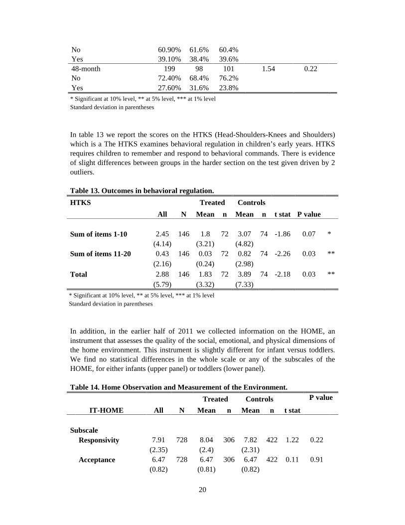
In table 13 we report the scores on the HTKS (Head-Shoulders-Knees and Shoulders) which is a The HTKS examines behavioral regulation in children’s early years. HTKS requires children to remember and respond to behavioral commands. There is evidence of slight differences between groups in the harder section on the test given driven by 2 outliers. Table 13. Outcomes in behavioral regulation.
HTKS
All N
Treated Controls
t stat P value
Mean n Mean n
Sum of items 1-10 2.45 146 1.8 72 3.07 74 -1.86 0.07 * (4.14) (3.21) (4.82) Sum of items 11-20 0.43 146 0.03 72 0.82 74 -2.26 0.03 ** (2.16) (0.24) (2.98)
Total 2.88 146 1.83 72 3.89 74 -2.18 0.03 **
(5.79) (3.32) (7.33) * Significant at 10% level, ** at 5% level, *** at 1% level Standard deviation in parentheses
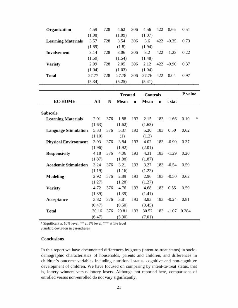
In addition, in the earlier half of 2011 we collected information on the HOME, an instrument that assesses the quality of the social, emotional, and physical dimensions of the home environment. This instrument is slightly different for infant versus toddlers. We find no statistical differences in the whole scale or any of the subscales of the HOME, for either infants (upper panel) or toddlers (lower panel). Table 14. Home Observation and Measurement of the Environment.
IT-HOME All N
Treated Controls
t stat
P value
Mean n Mean n Subscale Responsivity 7.91 728 8.04 306 7.82 422 1.22 0.22 (2.35) (2.4) (2.31) Acceptance 6.47 728 6.47 306 6.47 422 0.11 0.91 (0.82) (0.81) (0.82)
* Significant at 10% level, ** at 5% level, *** at 1% level Standard deviation in parentheses
Conclusions In this report we have documented differences by group (intent-to-treat status) in socio-demographic characteristics of households, parents and children, and differences in children’s outcome variables including nutritional status, cognitive and non-cognitive development of children. We have focused on comparing by intent-to-treat status, that is, lottery winners versus lottery losers. Although not reported here, comparisons of enrolled versus non-enrolled do not vary significantly.
22
The results indicate that for the most part, there are no significant differences by group status. This implies that random assignment to treatment was carried out successfully, and on average, both of our sample groups are similar to each other. Very few differences emerge, with some differences favoring one group and some favoring the other. Overall, we find there is no systematic bias in favor of either group to be concerned about when we estimate program impact further along this study.