1 First draft: November 2004 This draft: May 2005 Not for quotation: Comments welcome The Value Premium and the CAPM Eugene F. Fama and Kenneth R. French * Abstract We examine (i) how value premiums vary with firm size, (ii) whether the CAPM explains value premiums, and (iii) whether in general average returns compensate β in the way predicted by the CAPM. Loughran’s (1997) evidence for a weak value premium among large firms is special to 1963-1995, U.S. stocks, and the book-to-market value-growth indicator. Ang and Chen’s (2005) evidence that the CAPM can explain U.S. value premiums is special to 1926-1963. The CAPM’s general problem is that variation in β unrelated to size and value-growth goes unrewarded throughout 1926-2004. This produces rejections of the model for 1926-1963 and 1963-2004. * Graduate School of Business, University of Chicago (Fama), and Amos Tuck School of Business, Dartmouth College (French). We received helpful comments from Eduardo Repetto and seminar participants at Emory University.
Transcript
1
First draft: November 2004 This draft: May 2005
Not for quotation: Comments welcome
The Value Premium and the CAPM
Eugene F. Fama and Kenneth R. French*
Abstract
We examine (i) how value premiums vary with firm size, (ii) whether the CAPM explains value
premiums, and (iii) whether in general average returns compensate β in the way predicted by the CAPM.
Loughran’s (1997) evidence for a weak value premium among large firms is special to 1963-1995, U.S.
stocks, and the book-to-market value-growth indicator. Ang and Chen’s (2005) evidence that the CAPM
can explain U.S. value premiums is special to 1926-1963. The CAPM’s general problem is that variation
in β unrelated to size and value-growth goes unrewarded throughout 1926-2004. This produces rejections
of the model for 1926-1963 and 1963-2004.
* Graduate School of Business, University of Chicago (Fama), and Amos Tuck School of Business, Dartmouth College (French). We received helpful comments from Eduardo Repetto and seminar participants at Emory University.
1
Fama and French (1992), among others, identify a value premium in U.S. stock returns for the
period after 1963; stocks with high ratios of book equity to the market value of equity (value stocks) have
higher average returns than stocks with low book-to-market ratios (growth stocks). Extending the tests
back to 1926, Davis, Fama and French (2000) document a value premium in the average returns of the
earlier period.
Perhaps more important, Fama and French (1993) find that the post-1963 value premium is left
unexplained by the Capital Asset Pricing Model (CAPM) of Sharpe (1964) and Lintner (1965). Ang and
Chen (2005) show, however, that the value premium of 1926-1963 is captured by the CAPM. They also
argue that when the tests allow for time-varying market βs, even the post-1963 period produces no
reliable evidence against a CAPM story for the value premium. Loughran (1997) argues that the value
premium of 1963-1995 is in any case restricted to small stocks.
This paper has three goals. The first is to provide a simple picture of how value premiums vary
with firm size. The second is to examine if and when market βs line up with value premiums in a way
that allows the premiums to be captured by the CAPM. The third goal is to examine whether variation in
β across stocks is in general related to average returns in the way predicted by the CAPM.
Our results on how the value premium varies with firm size are easily summarized. Loughran’s
(1997) evidence that there is no value premium among large stocks seems special to (i) the post-1963
period, (ii) using the book-to-market ratio as the value-growth indicator, and (iii) restricting the tests to
U.S. stocks. During the earlier 1926-1963 period the value premium is near identical for small and big
U.S. stocks. When we use earnings-price ratios (E/P) rather than book-to-market ratios (B/M) to separate
value and growth stocks, 1963-2004 also produces little difference between value premiums for small and
big U.S. stocks. As another out-of-sample test, we examine international value premiums for 1975-2004
from 14 major markets outside the U.S. When we sort international stocks on either B/M or E/P, there is
again little difference between the value premiums for small and big stocks.
The evidence on U.S. value premiums and the CAPM is a bit more complicated. The overall
value premium in U.S. average returns is similar before and after 1963, but, like Franzoni (2001), we find
2
that market βs change dramatically. During the later period, value stocks have lower βs than growth
stocks – the reverse of what the CAPM needs to explain the value premium. As a result, the CAPM is
rejected for 1963-2004, whether or not one allows for time-varying βs. During 1926-1963, however,
value stocks have higher βs than growth stocks, and, like Ang and Chen (2005), we find that the value
premiums of the earlier period are captured near perfectly by the CAPM.
Given its success with the value premiums of 1926-1963, it is tempting to infer that the CAPM
provides a good description of average returns before 1963. It does not. The CAPM says that all
variation in β across stocks is compensated in the same way in expected returns. Fama and French (1992)
find that when portfolios are formed on size and β, variation in β related to size shows up in average
returns, but variation in β unrelated to size seems to go unrewarded. This suggests that, contradicting the
CAPM, it is size or a non-β risk related to size that counts, not β. The tests here extend this result. When
we form portfolios on size, B/M, and β, we find that variation in β related to size and B/M is compensated
in average returns for 1928-1963, but variation in β unrelated to size and B/M goes unrewarded during
1928-1963, indeed throughout the sample period. As a result, CAPM pricing is rejected for portfolios
formed on size, B/M, and β, for 1928-1963 as well as for 1963-2004. We conclude that it is size and B/M
or risks related to them, and not β, that are rewarded in average returns.
Finally, our evidence that variation in β unrelated to size and B/M is unrewarded in average
returns is as strong for big stocks as for small stocks. This should lay to rest the common claim that
empirical violations of the CAPM are inconsequential because they are limited to small stocks and thus
small fractions of invested wealth.
Our story proceeds as follows. Section I studies the relation between the value premium and firm
size. CAPM explanations of the value premium are examined in section II. Section III explores the
general problem for the CAPM created by variation in β unrelated to the size and value-growth
characteristics of firms. Section IV concludes.
3
I. Is there a Value Premium among Big Stocks?
Loughran (1997) contends that the value premium is limited to small stocks. For initial
perspective on this issue, we examine variants of VMG (also known as HML), the monthly value-growth
return of the three-factor model of Fama and French (1993). We construct VMG by forming six
portfolios on size (market capitalization, i.e., price times shares outstanding, henceforth called market
cap) and book-to-market equity (B/M). At the end of June each year from 1926 to 2004, we sort NYSE,
AMEX (after 1962), and (after 1972) Nasdaq firms with positive book equity into two size groups and
three B/M groups. Firms below the NYSE median size are small (S) and those above are big (B). We
assign firms to growth (G), neutral (N), and value (V) groups if their B/M is in the bottom 30%, middle
40%, or top 30% of NYSE B/M. The six portfolios, small and big growth (SG and BG), small and big
neutral (SN and BN), and small and big value (SV and BV), are the intersection of these sorts. The data
sources and calculation of book equity follow Davis, Fama, and French (2000), except that the NYSE
sample, extending back to 1926, now includes all NYSE firms, not just industrials.
The six value-weight size-B/M portfolios are the components of the monthly size and value-
growth returns of the Fama-French three-factor model. The size factor, SMB (small minus big), is the
simple average of the monthly returns on the three small stock portfolios minus the average of the returns
on the three big stock portfolios,
(1) SMB = (SG + SN + SV)/3 - (BG + BN + BV)/3.
The value-growth factor, VMG (value minus growth), is the simple average of the monthly
returns on the two value portfolios minus the average of the returns on the two growth portfolios,
(2) VMG = (SV + BV)/2 - (SG + BG)/2.
To test whether the value premium in average returns is special to small stocks, we split VMG
into its small stock and big stock components,
(3) VMGS = SV - SG and VMGB = BV - BG.
4
A. The Value Premium in Small and Big Stock Returns
Table 1 shows summary statistics for the monthly market excess return, RM-RF (the return on the
value-weight portfolio of the NYSE, AMEX, and Nasdaq stocks in our sample minus the one-month
Treasury bill rate), and the SMB, VMG, VMGS, and VMGB returns. Summary statistics for returns on
the six size-B/M portfolios used to construct SMB and VMG are also shown. The sample period is
7/1926-12/2004 (henceforth 26-04), but we also show results for 7/1926-6/1963 and 7/1963-12/2004
(henceforth 26-63 and 63-04). July 1963 is the start date of the tests in Fama and French (1992, 1993), so
26-63 is “out-of-sample” relative to early studies of the value premium.
The size premium in average returns is similar in the two subperiods. The average SMB return
for 26-63 is 0.20% per month versus 0.24% for 63-04. It takes the power of the full 26-04 sample period
to push the average premium (0.23%) just over the two standard error barrier (t = 2.06).
The overall value premium is also similar for the two subperiods of 26-04. The average VMG
return is 0.35% per month for 26-63 and 0.44% for 63-04. The average VMG return for 63-04 is 3.34
standard errors from zero, but the average for 26-63 is only 1.78 standard errors from zero. Under the
assumption that the standard deviations are equal, a comparison of means test shows, however, that the
premiums for 26-63 and 63-04 differ by just 0.38 standard errors, so the premium for the full 26-04
period is the best evidence on whether there is a value premium in expected returns. The 26-04 premium,
0.40% per month, is a healthy 3.43 standard errors from zero.
Confirming Loughran (1997) and earlier evidence in Fama and French (1993), the value premium
for 63-04 is larger for small stocks, 0.60% per month (t = 3.97), versus 0.26% (t = 1.87) for big stocks.
But for 26-63, the value premium is near identical for small and big stocks (0.35% and 0.36% per month).
Note that the difference between the small and big stock value premiums for 26-63 is largely due to an
increase in the premium for small stocks, from 0.35% to 0.60%; there is a smaller decline, from 0.36% to
0.26%, for big stocks. More important, a comparison of means test on the monthly VMGB returns shows
that the big stock value premium for 63-04 is just -0.37 standard errors from the premium for 26-63, so
there is no evidence of a change in the expected premium. The VMGB average return for the full 26-04
5
period, 0.31% per month (t = 2.23), is then the best evidence on the existence of a value premium in big
stock expected returns. In short, there does seem to be a value premium in the expected returns on big
stocks.
Still, the value premium in the average returns of 26-04 is 55% larger for small stocks (0.48% per
month) than for big stocks (0.31%). And the average of the time-series of differences between VMGS
and VMGB returns is 1.60 standard errors from zero. Thus, the power of the full sample period says that
there are value premiums in the expected returns on small and big stocks, but there is a hint that the
expected premium is larger for small stocks.
B. Finer Size Sorts
Table 1 classifies stocks above the NYSE median market cap as big. To be more comparable
with Loughran (1997), we next examine value premiums for a finer size grid. We use the 25 portfolios of
Fama and French (1993), formed as the intersection of independent sorts of stocks in June each year into
NYSE size and B/M quintiles. There is a problem, however. During 26-63 the portfolio for the largest
size and highest B/M quintiles often has no stocks, and the portfolio for the smallest size and lowest B/M
quintiles is also thin. To have at least ten stocks in each portfolio, the tests must be limited to 63-04.
Table 2 summarizes characteristics of the 25 size-B/M portfolios of 63-04, specifically, averages
across months of (i) number of firms, (ii) average firm size (market cap), and (iii) percent of total market
cap. A striking result is the skewness of percents of market cap across both size and B/M quintiles. By
count, the smallest size quintile on average contains more than half of total NYSE, AMEX, and Nasdaq
stocks. But these smallest stocks (micro-caps) are tiny and together they account for less than 3.0 percent
of total market cap. In contrast, there are on average just 295 stocks in the largest size quintile, but these
mega-caps account for about three-quarters of total market cap. The percent of total market cap falls
sharply, from 73.6% to 13.2% for the second largest size quintile and 6.5% for the third.
The drop is not as dramatic, but percent of market cap also falls across B/M quintiles. The lowest
B/M quintile (extreme growth stocks) on average accounts for 40.3% of total market cap, versus 8.1% for
6
the highest B/M quintile (extreme value stocks). The decline in percent of market cap across B/M
quintiles is steepest in the largest size quintile. Among these mega-caps, the lowest B/M portfolio
accounts for an impressive 32.8% of total market cap, versus 4.7% for the highest B/M portfolio. This
sharp decline has two sources: (i) on average the extreme growth mega-cap portfolio has about four times
as many stocks as the extreme value mega-cap portfolio, and (ii) though in the same size quintile, mega-
cap extreme growth stocks are about twice as large as mega-cap extreme value stocks. In contrast, there
is no clear relation between size and B/M in size quintiles below the largest. Except for the smallest size
quintile, however, all size groups share the result that growth stocks are more numerous than value stocks.
For perspective on the returns examined next, an important result in Table 2 is the paucity of
firms that are both large and in the extreme value group. On average, only 26 firms in the size quintile of
the largest firms are in the highest B/M quintile, and only 35 firms in the next largest size quintile are in
the highest B/M quintile. This is not surprising. Firms that are large in terms of market cap are likely to
have high stock prices and so are unlikely to be extreme value (high B/M) firms.
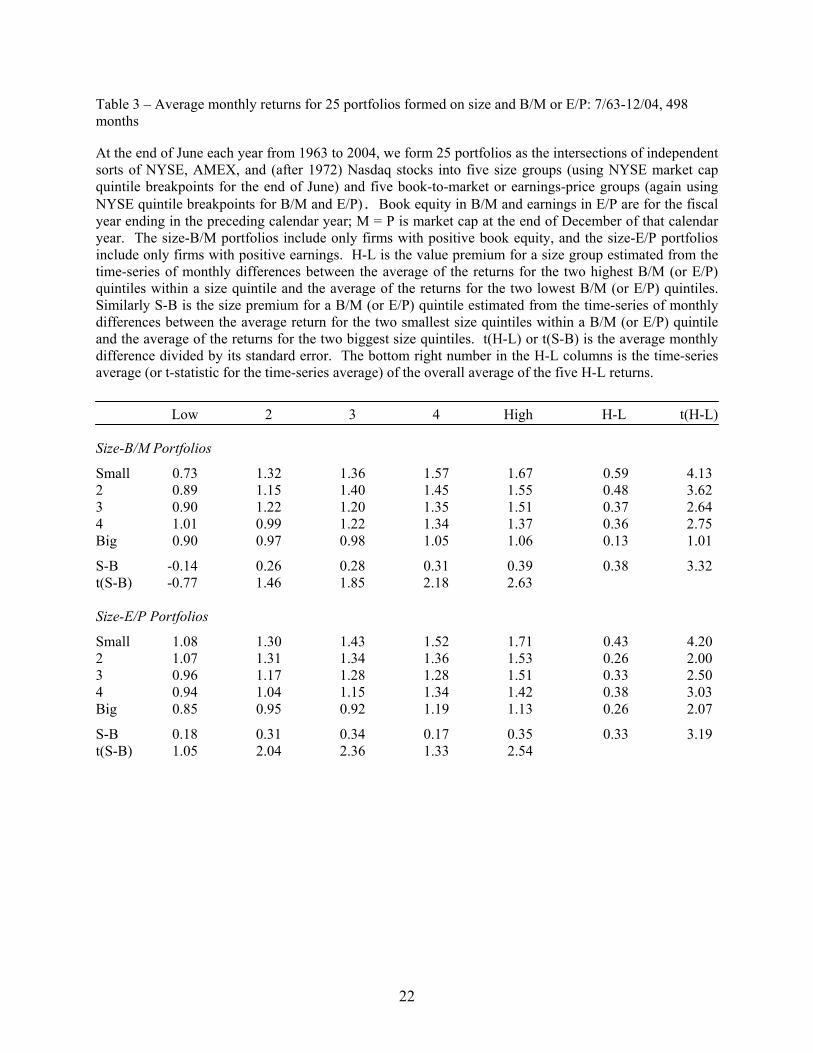
Table 3 shows average returns for 63-04 for the 25 size-B/M portfolios, along with value
premiums within size quintiles, and size premiums within B/M quintiles. The value premium for a size
quintile is the difference between the average return on the two highest B/M portfolios and the average
return on the two lowest B/M portfolios of the size quintile. Similarly, the size premium for a B/M
quintile is the difference between the average returns on the two smallest and the two biggest size
portfolios of the B/M quintile. We use four portfolios (rather than the extremes of each group) to estimate
premiums because, as noted above, some extreme portfolios are undiversified.
When value and growth are defined by sorts on B/M, the value premiums in average returns
decline monotonically from smaller to bigger size quintiles. For the size quintile containing the largest
firms (mega-caps), the value premium is only 0.13% per month, and about one standard error from zero.
The value premiums of the remaining four size groups are, however, economically and statistically
substantial. They range from 0.36% to 0.59% per month and are more than 2.6 standard errors from zero.
7
Even in the quintile containing the largest firms, average returns increase monotonically from lower
(growth) to higher (value) B/M quintiles.
The evidence for a weak value premium in the largest size quintile depends a lot on using B/M to
identify value and growth stocks. Table 3 also shows value premiums within size quintiles for 25
portfolios formed on size and earnings-price ratios (E/P). These portfolios are formed in the same way as
the 25 size-B/M portfolios, except that we exclude firms with negative earnings rather than negative book
equity, and we use E/P rather than B/M as the value-growth indicator. The effect of this change is to tone
down if not wipe out the decline in the value premium with firm size. The smallest size quintile still
produces the largest value premium. But any decline in value premiums with size is far from monotonic.
The largest size quintile produces the same value premium as the second smallest (0.26% per month), and
the second largest size quintile produces a value premium (0.38% per month) close to that for the smallest
size quintile (0.43%). Perhaps most important, when E/P is the value-growth indicator, the value
premiums for all size groups are more than two standard errors from zero.
There are two interesting changes in average returns when firms are sorted on E/P rather than
B/M. Most striking is the increase in average returns for extreme growth (low E/P) stocks in the two
smallest size quintiles, which acts to reduce the value premiums for these size groups, and so bring the
premiums closer to those of other size groups. In other words, the larger value premiums for small stocks
observed when B/M is the value-growth indicator are due more to lower returns on small growth stocks
than to higher returns on small value stocks. Using E/P as the value-growth indicator also reduces
average returns for the two extreme growth portfolios in the largest size quintile and increases average
returns on the two extreme value portfolios, leading to a higher value premium which is now more than
two standard errors from zero.
Why do the return results change for the E/P sorts? The answer traces largely to firms with
negative earnings (excluded from the E/P sorts in Table 3). Prior to July 1978, the two biggest size
quintiles often have no firms with negative earnings, but thereafter all size quintiles have at least one
unprofitable firm. Table 4 shows that during 78-04, on average more than 25% of listed firms have
8
negative earnings. But the incidence is skewed. On average, 83% of the firms with negative earnings are
in the smallest size quintile, and they are more than one-third of all such micro-cap stocks. In the biggest
size quintile on average less than 6% of firms are unprofitable.
Table 4 also shows that in the two largest size quintiles, the returns of firms with negative
earnings are rather high. But in the three smallest size quintiles, firms with negative earnings have by far
the lowest average returns. Thus, in the size quintiles where they are numerous, the returns of firms with
negative earnings are poor. Comparing the 78-04 returns for the sorts on E/P and B/M in Table 4 then
suggests that in the two smallest size quintiles, the low returns of firms with negative earnings act mostly
to lower the returns of firms in the lowest B/M quintile. This raises the estimates of the value premiums
for these size quintiles and creates a strong inverse relation between size and the value premium, which is
not observed when E/P is the value-growth indicator. (Detailed results, not shown, obtained when the 25
size-B/M portfolios are split into positive and negative earnings portfolios, confirm these inferences.)
Though not our central focus, it is interesting to note that the monotonic decline in the value
premium from smaller to bigger size groups observed in the B/M sorts in Table 3 corresponds to a
monotonic increase in size premiums from lower to higher B/M groups. But this pattern in size premiums
for 63-04 is almost non-existent when the value-growth indicator is E/P. Even the extreme growth
(lowest positive) E/P quintile produces a hint of a size premium for 63-04, absent in the B/M sorts.
C. International Results
International returns provide an out-of-sample test of whether there is a value premium among
large stocks. Using Morgan Stanley Capital International (MSCI), we construct 25 size-B/M portfolios
and 25 size-E/P portfolios using merged data for 14 markets outside the U.S.1 To establish an exact size
parallel with the U.S. results, the breaks for size quintiles are the same NYSE market cap breaks used for
the U.S. Since international accounting methods differ from those of the U.S., the quintile breaks for
1 We thank Dimensional Fund Advisors for purchasing these data on our behalf.
9
B/M and E/P use the annual cross-sections of the ratios for international stocks. We can report, however,
that using U.S. breaks for the ratios has no effect on inferences.
An advantage of the MSCI data is that they are free of survivor bias; firms that die remain in the
historical sample. Moreover, the annual accounting data shown at the end of any month are the most
recently reported, so they are publicly available. A disadvantage of MSCI is that the sample covers only
1975-2004. And though the firms included account for more than 80% of the market cap of the 14
markets, the small end of the size spectrum is sparse, and there are few firms in the micro-cap quintile.
Thus, in presenting the international results, we show only two size groups, (i) the top size quintile
(mega-caps), and (ii) all remaining firms. This is not a problem since our main interest is whether there is
a value premium for the largest stocks and whether it is smaller than for other stocks.
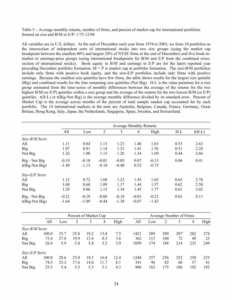
The international sample resembles the U.S. sample in many ways. For example, there are on
average only about 350 mega-cap firms in the international sample, versus almost three times as many
smaller firms, but the mega-caps account for about three quarters of the sample’s total market cap
(Table 5). Again, more of the sample’s market cap comes from growth stocks. But in the international
sample, this result is due entirely to mega-caps, where growth stocks outnumber value stocks by more
than two to one.
Most important, Table 5 documents strong value premiums in international returns. (As in the
U.S. results, international value premiums are estimated as the difference between the average returns for
the two extreme value and the two extreme growth portfolios of a group.) When B/M is the value-growth
indicator, the overall value-weight international value premium is 0.53% per month (t = 2.63); it is an
even larger 0.65% per month (t = 2.78) for E/P groupings. (See also Fama and French 1998.)
The new evidence in Table 5 centers on the value premium for very large stocks. When we sort
on B/M, the value premium for mega-caps is six basis points per month larger than it is for all smaller
stocks, but the difference is indistinguishable from zero (t = 0.41). Sorting on E/P, the premiums for the
two size groups are virtually identical. In short, international returns show economically and statistically
strong value premiums, and they are as large among the biggest stocks as among smaller stocks.
10
D. Bottom Line
In sum, when we use B/M to identify value and growth stocks in the U.S., value premiums for
63-04 are smaller for large firms. Although there are large and statistically reliable value premiums in the
four smaller size quintiles, the premium for the largest size quintile, 0.13% per month, is just 1.01
standard errors from zero. When we sort on E/P rather than B/M, however, we find a strong value
premium in even the largest size quintile and little relation between the value premium and firm size. The
evidence for 26-63 (Table 1) is also relevant. Though we only have a 2x3 size-B/M grid for the earlier
period, if the value premium is negatively related to size, small stocks should produce a bigger premium
than big stocks. But the premiums for small and big stocks for 26-63 (0.35% and 0.36% per month) are
near identical. Finally, whether we sort on B/M or E/P, international average returns for 75-04 show
strong value premiums that are at least as large for mega-caps as for smaller stocks. All this suggests that
the weak relation between B/M and average returns observed for the largest U.S. size quintile for 63-04
may be a random aberration.
II. The Value Premium and the CAPM
Does the CAPM explain the value premium in average returns? In Fama and French (1993), we
conclude that the answer is no for the period after 1963. Ang and Chen (2005) find, however, that the
CAPM explains the premium of 26-63. The plot of year-by-year betas for VMG in Figure 1 suggests an
explanation. As Franzoni (2001) emphasizes, the market β for VMG falls during the sample period. The
β for 26-63 (Table 6) is large and positive, 0.35 (t = 13.62), and the β for 63-04 is strongly negative, -0.28
(t = -10.31). Because the β for value stocks is lower than the β for growth stocks in the later period, the
CAPM cannot explain the positive value premium for 63-04. But the beta for VMG is positive for 26-63,
so the positive value premium of this period may be consistent with the CAPM.
11
A. Time Series Tests
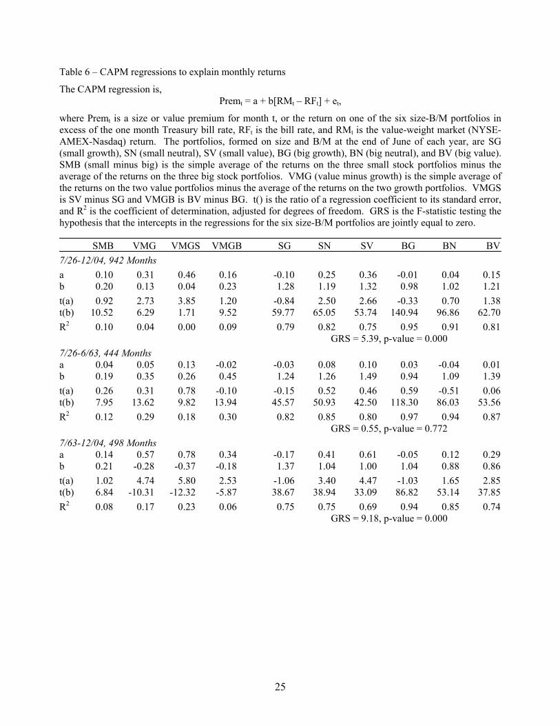
The regressions of VMG, VMGS, and VMGB returns on the excess market return in Table 6 test
whether the CAPM can explain value premiums. In a CAPM world, the true intercepts in these
regressions are zero. Confirming Fama and French (1996), the CAPM regression to explain VMG returns
for 63-04 produces an intercept, 0.57% per month (t = 4.74), that easily rejects the CAPM. Since the
market β for VMG for 63-04 is negative (-0.28, t = -10.31), the intercept in the CAPM regression for
VMG in Table 6 is larger than the (already large) average VMG return in Table 1.
The value premium for big stocks for 63-04, 0.26% per month, is economically large but slightly
less than two standard errors from zero (t = 1.87, Table 1). The negative market β for VMGB, however,
leads to a CAPM regression intercept, 0.34%, that is larger and 2.53 standard errors from zero (Table 6).
Thus, even for big stocks (which for VMGB is all stocks above the NYSE median market cap) there is
reliable evidence that the CAPM cannot explain the value premium of 63-04. But the value premium for
small stocks does produce a stronger CAPM rejection. The intercept in the CAPM regression for VMGS
is 0.78% per month (t = 5.80).
To complete the picture, Table 6 shows CAPM regressions to explain excess returns on the six
size-B/M portfolios in SMB and VMG. In the regressions for 63-04, the F-test of Gibbons, Ross, and
Shanken (GRS 1989) cleanly rejects the hypothesis that the CAPM can explain the average returns on
these portfolios. The portfolios that seem to cause trouble for the CAPM are the small value portfolio SV
(CAPM intercept 0.61% per month, t = 4.47), the small neutral portfolio SN (intercept 0.41%, t = 3.40),
and the big value portfolio BV (intercept 0.29%, t = 2.85). In contrast, the CAPM intercepts for the two
growth portfolios, SG and BG, are only about one standard error below zero. Thus, the power to reject
the CAPM in 63-04 seems to come more from the high returns on value portfolios than from the lower
returns on growth portfolios.
The success of the CAPM for the earlier 26-63 period documented by Ang and Chen (2005) is
confirmed in Table 6. Despite average VMG returns that are similar for 26-63 and 63-04, a dramatic
change in the market β for VMG, from negative -0.28 for 63-04 to positive 0.35 for 26-63, leads to an
12
intercept for 26-63 (0.05% per month, t = 0.31) quite consistent with CAPM pricing. Splitting VMG into
its small and big stock components, VMGS and VMGB, reinforces this conclusion. Table 6 shows that
during 26-63, the CAPM also explains average returns on the six size-B/M portfolios. The CAPM
intercepts for the six portfolios are all within 0.60 standard errors of zero, and the GRS test produces a p-
value (0.77) quite consistent with CAPM pricing.
Finally, though not our main interest, Table 6 also confirms earlier evidence (Chan and Chen
1988, Fama and French 1996) that the size premium in average returns is consistent with CAPM pricing.
The market β for SMB for 26-63, 0.19, is close to that for 63-04, 0.21. Since SMB’s market β does not
seem to change from the earlier to the later period, the full sample period is the best evidence on whether
the CAPM explains the average SMB return. In the CAPM regression for SMB for 26-04, the intercept is
0.10% (t = 0.92). In short, Table 1 identifies a reliable average size premium for 26-04, but Table 6 says
that about half of it is absorbed by SMB’s market β, leaving little evidence against CAPM pricing as the
explanation for the premium in the average returns on small stocks.
B. Time-Varying βs
Ang and Chen (2005) argue that when beta is allowed to vary through time, even the period after
July 1963 produces no reliable evidence that the CAPM fails to explain value premiums. The market βs
for VMG, VMGS, and VMGB in Figure 1, estimated for annual periods beginning in 7/1926, show that
there is indeed substantial variation through time in the βs of value premiums. The βs bounce around a
lot, which is not surprising given that each uses just 12 monthly returns. But, confirming Franzoni
(2001), the dominant pattern is down; the β estimates are near their highest values early in the sample
period and near their lowest toward the end. The annual βs for the components of VMG in Figure 2
provide supporting details. The βs of the two value portfolios (again with lots of variation) largely just
seem to fall, starting the period far above the β estimates for the growth portfolios and ending far below.
Ang and Chen (2005) model variation in the market βs of value premiums as slowly mean
reverting first order autoregressions (AR1s) in a highly parameterized latent variable model that also
13
includes assumptions about how the expected value of the excess market return and its volatility vary
through time. We are wary of imposing so much structure on the process assumed to generate β and the
other central variables of the CAPM. Instead, we use a simple non-parametric approach, less exposed to
specification issues, to accommodate time-varying βs. We estimate CAPM regressions for the full 26-04
period that use slope dummies to allow for periodic changes in market β. We examine four alternatives:
(i) a constant β for the period, (ii) a single break in β in 7/1963, (iii) βs for non-overlapping periods that,
except for the last, are five years in length, and (iv) βs that change annually (as in Figures 1 and 2) at the
June portfolio formation point. To judge which is best, we examine regression R2, adjusted for degrees of
freedom. If shortening the period over which β is assumed constant increases R2, we infer that picking up
more variation in true βs more than compensates for the loss in degrees of freedom.
The message from these regressions (Panel A of Table 7) is clear. For every portfolio, shortening
the estimation interval for β increases R2 or leaves it unchanged. We infer that allowing β to change each
year when portfolios are rebalanced is best among the alternatives examined. This is perhaps not
surprising since portfolio compositions change when the portfolios are reformed at the end of each June.
Allowing β to change every year weakens the evidence against CAPM pricing of the value
premium for the full sample period. Panel A of Table 7 shows that with annual changes in β, the intercept
in the CAPM regression for VMG for 26-04 is 0.20% per month (t = 2.05), versus 0.31% (t = 2.73) with
no change in β, and 0.37% (t = 3.79) when β is allowed to change every five years. And the rejection is
mostly due to small stocks. With annual changes in β, the intercept in the full-period CAPM regression
for VMGB is positive but just 0.08% per month (t = 0.68), versus 0.31% per month (t = 2.89) for VMGS.
Allowing annual changes in β continues to produce a strong rejection of the CAPM in the GRS test for
the six size-B/M components of SMB and VMG for 26-04 (Table 7).
C. The CAPM before and after July 1963
The full-period regressions in Panel A of Table 7 reject CAPM pricing as an explanation for the
average VMG return, but the split sample regressions in Table 6 open the possibility that the rejection is
14
entirely due to 63-04. If so, full-period constant intercept regressions are misleading. In imposing one
intercept for 26-04, they dilute both the success of the CAPM during 26-63 and its failure during 63-04.
The CAPM is such an elegantly simple paradigm, it behooves us to examine in detail whether it had a
golden age during 26-63.
Panel B of Table 7 shows full-period CAPM regressions for the three value premiums that allow
market βs to change every year, but also include a dummy variable for 63-04 in addition to the (full-
period) intercept. The intercepts, a26, are the average returns for 26-63 left unexplained by the CAPM.
The coefficients on the dummy variable for 63-04, a63-a26, measure differences between CAPM
intercepts for 63-04 and 26-63. The dummy variable thus tells us whether the CAPM’s ability to explain
value premiums is different in the two periods. The answer is a clear yes. The coefficients on the 63-04
dummy in the regressions for VMG, VMGS, and VMGB are 2.97, 3.19, and 1.96 standard errors from
zero. In contrast, the intercepts are within one standard error of zero. Thus, allowing βs to change
annually confirms the inference that the CAPM can explain the value premiums of 26-63, but also
indicates that 63-04 is a different matter.
If the CAPM’s inability to explain value premiums is special to 63-04, we get a clearer picture of
the problem by estimating separate (rather than marginal) CAPM intercepts for 26-63 and 63-04. Panel C
of Table 7 shows full-period CAPM regressions for VMG, VMGS, and VMGB that allow βs to change
every year and include dummy variables for 26-63 and 63-04 but no full-period intercept.2 These tests
reject CAPM pricing for 63-04, cleanly for VMG and VMGS (intercepts of 0.46% and 0.62% per month,
t = 3.52 and t = 4.29) and marginally for VMGB (an intercept of 0.28%, t = 1.83). The regressions for the
six size-B/M portfolios are also bad news for CAPM pricing during 63-04. The 63-04 intercepts for SV,
SN, and BV (0.59%, 0.45%, and 0.22% per month) in Panel C of Table 7 are economically large and
3.52, 3.44, and 1.84 standard errors from zero. Lewellen and Nagel (2005) use a different approach to
deal with time varying betas, but their inferences about the CAPM are consistent with ours.
2 The annual βs from the regressions in Panels B and C of Table 7 are in Figures 1 and 2. They are near identical to the annual βs from the regressions in Panel A of Table 7, which do not allow for changes in the intercepts during the sample period.
15
In sum, allowing βs to change annually leaves us with the conclusion that the CAPM can explain
the value premiums in the average returns of 26-63, but it fails to capture the value premiums of 63-04.
III. β Sorts and the CAPM
Do the small CAPM intercepts for the value premiums of 26-63 imply that the CAPM explains
expected stock returns during this period? Not necessarily. There is an alternative hypothesis that, unlike
the CAPM, describes average returns for 63-04 as well as for 26-63. Specifically, expected returns vary
with B/M (or a risk related to B/M), not with β. Value (high B/M) stocks have higher expected returns
regardless of their βs. And β seems to be rewarded in average returns only when it is positively correlated
with B/M (or size). The value premiums of 63-04 favor this story over the CAPM. The positive value
premiums of this period line up with positive spreads in B/M and not with the negative spreads in β.
Distinguishing between the two stories in the returns for 26-63 is more challenging. Since both
B/M and β are higher for value stocks than for growth stocks, the positive value premiums for 26-63 are
consistent with both the CAPM and our alternative B/M explanation. One way to distinguish between the
two is to create variation in β that is independent of the variation in B/M (Daniel and Titman 1997). We
do this by splitting each of the six size-B/M portfolios (used to construct SMB and VMG) into high and
low β portfolios each year, using βs estimated with two to five years (as available) of past monthly
returns. We then calculate the differences between the value weight returns on the six high β and the six
low β portfolios. We also calculate an overall difference, HBmLB, which is the simple average of the six
high β minus low β return spreads. HBmLB is thus a diversified return that provides an overall summary
of the β premium within portfolios formed on size and B/M. Since 1926 and 1927 are lost when we
estimate the βs used to form the first spread portfolios in June of 1928, the sample period for these tests is
28-04 (July 1928 to December 2004).
Table 8 shows that splitting the size-B/M portfolios on estimates of β produces small spreads in
average returns. The overall HBmLB average return is only 0.04% per month (t = 0.40) for the full 28-04
16
period, 0.09% (t = 0.56) for 28-63, and -0.00% (t = -0.04) for 63-04. These tiny average return spreads
are ominous for the CAPM.
The regressions in Table 8 confirm that the average returns on the β-spread portfolios violate the
CAPM. The β splits of the size-B/M portfolios produce large spreads in post formation βs. The estimates
for the full 28-04 period range from 0.33 (t = 15.47) to 0.52 (t = 23.49). The βs for the spread portfolios
also do not change much from 28-63 to 63-04, and the overall spread portfolio, HBmLB, has the same
post formation β, 0.42, in both periods. Large positive market βs and tiny average return spreads combine
to produce large negative intercepts in the CAPM regressions for the β-spread portfolios in Table 8.
Twenty of 21 intercepts are negative and many are more than two standard errors below zero.
Because of its diversification, the overall HBmLB return has the lowest variance among the
spread portfolio returns, and the CAPM regressions to explain the HBmLB return have the lowest
residual variances. HBmLB thus provides a powerful overall test of whether the CAPM can explain
average returns on the β spread portfolios. The HBmLB intercept for 28-04, -0.22% per month (t =
-3.31), strongly rejects the CAPM; the intercepts for 28-63 and 63-04 are similar (-0.24% and -0.20% per
month) and more than 2.3 standard errors below zero. The GRS tests on the intercepts from the CAPM
regressions for the six components of HBmLB also reject CAPM pricing.
In the end, we have four pieces of evidence on the CAPM. (i) Throughout 26-04, small firms
have larger market βs than big firms, and the CAPM captures much of the size premium in average
returns. (ii) During 26-63, there is a positive correlation between β and B/M, and the value premiums of
this period are also consistent with the CAPM. (iii) But the CAPM cannot explain the value premiums of
63-04, when high B/M (value) stocks have lower βs than low B/M (growth) stocks. (iv) Throughout
26-04, variation in β within portfolios formed on size and B/M is not compensated in the manner
predicted by the CAPM – if at all. Taken together, these four findings suggest that there is little if any
compensation for differences in beta unrelated to size and B/M. Apparently, it is not beta, but size and
B/M or risks related to them that count in expected returns.
17
Fans of the CAPM sometimes claim that violations of the model are of little consequence because
they are limited to stocks that account for little total market cap. This conclusion stems from results like
those in Table 6, where the big growth and big neutral portfolios, BG and BN, which on average account
for more than 80% of total market cap, do not suggest violations of the CAPM. But Table 8 identifies
lots of variation in β within BG and BN that does not show up in average returns. Although the β-spread
portfolios for BG and BN produce large β estimates for 28-04, 0.39 (t = 26.28) and 0.42 (t = 24.85), their
average returns are close to zero, 0.00% (t = 0.00) for BG and 0.07% (t = 0.60) for BN. It is thus not
surprising that the β-spread portfolios for BG and BN produce negative CAPM regression intercepts that
reject the model. The intercepts for 28-04 are -0.25% (BG) and -0.19% (BN) per month (t = -2.96 and t =
-2.02), and they are outdone in size and significance only by the β-spread portfolio for SG. In short, the
evidence that variation in β unrelated to size and B/M goes unrewarded in average returns is not restricted
to small stocks or small fractions of total market cap.
IV. Conclusions
We examine (i) how value premiums vary with firm size, (ii) whether the CAPM explains value
premiums, and (iii) whether in general average returns compensate differences in β in the way predicted
by the CAPM.
Loughran’s (1997) evidence that there is no value premium among the largest stocks seems to be
special to (i) the U.S., (ii) the post-1963 period, and (iii) using the book-to-market ratio as the value-
growth indicator. During the earlier 1926-1963 period, the value premium is near identical for small and
big U.S. stocks. When we use E/P rather than B/M to separate value and growth stocks, 1963-2004 also
produces strong value premiums for all size quintiles and little difference between value premiums for big
and small U.S. stocks. And international value premiums for 1975-2004 from 14 major markets outside
the U.S. are as large for mega-cap stocks as for smaller stocks. These results suggest that the weak
relation between B/M and average returns observed for the largest U.S. size quintile during 63-04 may be
a random aberration, due perhaps to the paucity of mega-cap value stocks.
18
The CAPM can explain the strong value premiums of 26-63, but not those of 63-04. During the
later period, growth stocks tend to have larger market βs than value stocks – the reverse of what the
CAPM requires to explain value premiums. A CAPM explanation of the value premiums of 63-04 is thus
rejected, with or without allowance for time-varying market βs. During the earlier 26-63 period,
however, value stocks have larger βs than growth stocks, and like Ang and Chen (2005) we find that the
CAPM captures the value premiums of this period near perfectly.
Unfortunately, the CAPM has a different and more general problem that overshadows its success
with the value premiums of 26-63. The CAPM says all differences in β are compensated in the same way
in expected returns. But when we form portfolios on size, B/M, and β, we find that variation in β related
to size and B/M is compensated in average returns for 1928-1963, but variation in β unrelated to size and
B/M goes unrewarded during 1928-1963 and throughout the sample period. As a result, CAPM pricing is
rejected for portfolios formed on size, B/M, and β, for 1928-1963 as well as for 1963-2004. And this
rejection of the CAPM is as strong for large stocks, which account for the lion’s share of market wealth,
as for small stocks.
The final scoreboard presents us with the following facts. During 26-63 the market βs of
portfolios formed on size and B/M line up with average returns in the manner predicted by the CAPM,
and size and value premiums are captured by the CAPM. But variation in β unrelated to size and B/M
seems to carry little or no premium. During 63-04, size and value premiums are similar to those of 26-63,
but along the value-growth dimension market βs no longer line up with average returns in the manner
predicted by the CAPM. And again, variation in β unrelated to size and B/M carries little or no premium.
Based on these results, we conclude that the CAPM has fatal problems throughout the 26-04
period. Specifically, size and B/M or risks related to them are important in expected returns, whether or
not they relate to β in a way that would support the CAPM, and β has little or no independent role. But
we expect challenges.
19
References Ang, Andrew, and Joseph Chen, 2005, The CAPM over the long run: 1926-2001, manuscript, Columbia
University, January. Chan, K. C., and Nai-fu Chen, 1988, An unconditional asset-pricing test and the role of firm size as an
instrumental variable for risk, Journal of Finance 43, 309-325. Daniel, Kent, and Sheridan Titman, 1997, Evidence on the characteristics of cross sectional variation in
stock returns, Journal of Finance 52, 1-33. Davis, James L., Eugene F. Fama, and Kenneth R. French, 2000, Characteristics, covariances, and
average returns: 1929-1997, Journal of Finance 55, 389-406. Fama, Eugene F., and Kenneth R. French, 1992, The cross-section of expected stock returns, Journal of
Finance 47, 427-465. Fama, Eugene F., and Kenneth R. French, 1993, Common risk factors in the returns on stocks and bonds,
Journal of Financial Economics 33, 3-56. Fama, Eugene F., and Kenneth R. French, 1996, Multifactor explanations of asset pricing anomalies,
Journal of Finance 51, 55-84. Fama, Eugene F., and Kenneth R. French, 1998, Value versus growth: The international evidence,
Journal of Finance, 53, 1975-1999. Franzoni, Francesco, 2001, Where is beta going? The riskiness of value and small stocks, PhD
dissertation, MIT. Gibbons, Michael R., Stephen A. Ross, and Jay Shanken, 1989, A test of the efficiency of a given
portfolio, Econometrica 57, 1121-1152. Lewellen, Jonathan, and Stefan Nagel, 2005, The conditional CAPM does not explain asset-pricing
anomalies, working paper, MIT. Lintner, John, 1965, The valuation of risk assets and the selection of risky investments in stock portfolios
and capital budgets, Review of Economics and Statistics 47, 13-37. Loughran, Tim, 1997, Book-to-market across firm size, exchange, and seasonality, Journal of Financial
and Quantitative Analysis 32, 249-268. Sharpe, William F., 1964. Capital asset prices: A theory of market equilibrium under conditions of risk,
Journal of Finance 19, 425-442.
20
Table 1 – Summary statistics for monthly returns on size and value factors and the size-B/M portfolios used to construct them At the end of June of each year from 1926 to 2004, we form six value-weight portfolios, SG, SN, SV, BG, BN, and BV. The portfolios are the intersections of independent sorts of NYSE, AMEX (after 1962), and Nasdaq (after 1972) stocks into two size groups, S (small, firms with June market cap below the NYSE median) and B (big, market cap above the NYSE median), and three book-to-market equity (B/M) groups, G (growth, firms in the bottom 30% of NYSE B/M), N (neutral, middle 40% of NYSE B/M), and V (value, high 30% of NYSE B/M). Book equity is Compustat’s total assets (data item 6), minus liabilities (181), plus balance sheet deferred taxes and investment tax credit (35) if available, minus (as available) liquidating (10), redemption (56), or carrying value (130) of preferred stock. In the B/M sorts in June of year t, book equity is for the fiscal year ending in the preceding calendar year, t-1, and market equity is market cap at the end of December of that calendar year. Only firms with positive book equity are used. The size premium, SMB (small minus big), is the simple average of the returns on the three small stock portfolios minus the average of the returns on the three big stock portfolios. The value premium, VMG (value minus growth), is the simple average of the returns on the two value portfolios minus the average of the returns on the two growth portfolios. VMGS is SV minus SG, VMGB is BV minus BG, and VMGS-B is VMGS minus VMGB. RM-RF is the difference between the value-weight market return and the one-month Treasury bill rate. The table shows means, standard deviations (Std Dev) and t-statistics for the mean (the ratio of the mean to its standard error). Factor Portfolios Size-B/M Portfolios RM-RF SMB VMG VMGS VMGB VMGS-B SG SN SV BG BN BV
Table 2 – Characteristics of 25 portfolios formed on size and B/M: 7/63-12/04, 498 months At the end of June each year from 1963 to 2004, we form 25 portfolios as the intersections of independent sorts of NYSE, AMEX, and (after 1972) Nasdaq stocks into five size groups (using NYSE market cap quintile breakpoints for the end of June) and five book-to-market groups (again using NYSE quintile breakpoints for B/M). Book equity in B/M is for the fiscal year ending in the preceding calendar year and market equity is market cap at the end of December of that calendar year. Firms with negative book equity are excluded. For each portfolio, the table shows averages across the months of 7/63-12/04 of (i) number of firms, (ii) average market cap, and (iii) percent of total market cap, which is the product of (i) and (ii) divided by the sum of these products across portfolios. The table also shows the average across years of B/M for each portfolio, where book equity and market equity for a given year are the sums for the firms in a portfolio. In the blocks for Number of Firms and Percent of Total Market Cap, Sum is the sum across rows or columns of the items in the column or row. Number of Firms Average Market Cap ($Millions) Low 2 3 4 High Sum Low 2 3 4 High Small 532 337 338 402 645 2255 39 42 40 36 27 2 163 117 114 103 79 576 186 188 191 189 185 3 121 88 81 67 48 405 444 452 453 456 464 4 100 75 64 53 35 327 1147 1142 1150 1160 1156 Big 108 66 52 43 26 295 10240 7658 6608 5454 5001 Sum 1025 682 649 669 832 3858 Percent of Total Market Cap Annual Sum B/Sum M Low 2 3 4 High Sum Low 2 3 4 High Small 0.7 0.5 0.5 0.5 0.7 2.9 0.27 0.57 0.77 1.02 1.77 2 1.1 0.8 0.8 0.7 0.5 3.8 0.27 0.54 0.76 1.00 1.66 3 1.9 1.4 1.3 1.1 0.8 6.5 0.27 0.54 0.75 1.00 1.62 4 3.9 2.9 2.6 2.2 1.5 13.2 0.27 0.55 0.75 1.02 1.62 Big 32.8 15.5 11.6 9.0 4.7 73.6 0.26 0.53 0.75 0.99 1.49 Sum 40.3 21.1 16.8 13.6 8.1 100.0
22
Table 3 – Average monthly returns for 25 portfolios formed on size and B/M or E/P: 7/63-12/04, 498 months At the end of June each year from 1963 to 2004, we form 25 portfolios as the intersections of independent sorts of NYSE, AMEX, and (after 1972) Nasdaq stocks into five size groups (using NYSE market cap quintile breakpoints for the end of June) and five book-to-market or earnings-price groups (again using NYSE quintile breakpoints for B/M and E/P). Book equity in B/M and earnings in E/P are for the fiscal year ending in the preceding calendar year; M = P is market cap at the end of December of that calendar year. The size-B/M portfolios include only firms with positive book equity, and the size-E/P portfolios include only firms with positive earnings. H-L is the value premium for a size group estimated from the time-series of monthly differences between the average of the returns for the two highest B/M (or E/P) quintiles within a size quintile and the average of the returns for the two lowest B/M (or E/P) quintiles. Similarly S-B is the size premium for a B/M (or E/P) quintile estimated from the time-series of monthly differences between the average return for the two smallest size quintiles within a B/M (or E/P) quintile and the average of the returns for the two biggest size quintiles. t(H-L) or t(S-B) is the average monthly difference divided by its standard error. The bottom right number in the H-L columns is the time-series average (or t-statistic for the time-series average) of the overall average of the five H-L returns.
Table 4 – Average monthly returns and number of firms for 25 size-B/M and 30 size-E/P portfolios: 7/78-12/04, 318 months At the end of each June, we form portfolios as the intersections of independent sorts of NYSE, AMEX, and Nasdaq stocks into five size groups (using NYSE market cap quintile breakpoints for the end of June) and five book-to-market or six earnings-price groups (again using NYSE quintile breakpoints for B/M and E/P). Book equity in B/M and earnings in E/P are for the fiscal year ending in the preceding calendar year; M = P is market cap at the end of December of that calendar year. The size-B/M portfolios do not include firms with negative book equity. H-L is the value premium for a size group estimated from the time-series of monthly differences between the average of the returns for the two highest B/M (or E/P) quintiles within a size quintile and the average of the returns for the two lowest B/M (or positive E/P) quintiles. Similarly S-B is the size premium for a B/M (or E/P) group estimated from the time-series of monthly differences between the average return for the two smallest size quintiles within a B/M (or E/P) group and the average of the returns for the two biggest size quintiles. t(H-L) or t(S-B) is the average monthly difference divided by its standard error. The bottom right number in the H-L columns is the time-series average (or t-statistic for the time-series average) of the overall average of the five H-L returns. Sum is the sum across rows or columns of the numbers in the column or row. Size-E/P Portfolios Size-B/M Portfolios
Neg Low 2 3 4 High H-L t(H-L) Low 2 3 4 High H-L t(H-L)
Table 5 – Average monthly returns, number of firms, and percent of market cap for international portfolios formed on size and B/M or E/P: 1/75-12/04 All variables are in U.S. dollars. At the end of December each year from 1974 to 2003, we form 10 portfolios as the intersection of independent sorts of international stocks into two size groups (using the market cap breakpoint between the smallest 80% and largest 20% of NYSE firms at the end of December) and five book-to-market or earnings-price groups (using international breakpoints for B/M and E/P from the combined cross-section of international stocks). Book equity in B/M and earnings in E/P are for the latest reported year preceding December portfolio formation; M = P is market cap at portfolio formation. The size-B/M portfolios include only firms with positive book equity, and the size-E/P portfolios include only firms with positive earnings. Because the smallest size quintiles have few firms, the table shows results for the largest size quintile (Big) and combined results for the four remaining size quintiles (Not Big). H-L is the value premium for a size group estimated from the time-series of monthly differences between the average of the returns for the two highest B/M (or E/P) quintiles within a size group and the average of the returns for the two lowest B/M (or E/P) quintiles. t(H-L) or t(Big-Not Big) is the average monthly difference divided by its standard error. Percent of Market Cap is the average across months of the percent of total sample market cap accounted for by each portfolio. The 14 international markets in the tests are Australia, Belgium, Canada, France, Germany, Great Britain, Hong Kong, Italy, Japan, the Netherlands, Singapore, Spain, Sweden, and Switzerland. Average Monthly Returns All Low 2 3 4 High H-L t(H-L)
Size-B/M Sorts All 1.11 0.84 1.13 1.23 1.40 1.63 0.53 2.63 Big 1.07 0.81 1.14 1.21 1.41 1.56 0.51 2.24 Not Big 1.26 1.00 1.15 1.26 1.34 1.69 0.44 2.66
Big - Not Big -0.19 -0.18 -0.01 -0.05 0.07 -0.13 0.06 0.41 t(Big-Not Big) -1.49 -1.13 -0.10 -0.40 0.52 -0.75
Size-E/P Sorts All 1.12 0.72 1.08 1.23 1.45 1.65 0.65 2.78 Big 1.08 0.68 1.09 1.17 1.44 1.57 0.62 2.50 Not Big 1.29 0.86 1.15 1.34 1.45 1.77 0.61 3.02
Big - Not Big -0.21 -0.18 -0.06 -0.18 -0.01 -0.21 0.01 0.11 t(Big-Not Big) -1.64 -1.09 -0.44 -1.38 -0.07 -1.42
Table 6 – CAPM regressions to explain monthly returns
The CAPM regression is, Premt = a + b[RMt – RFt] + et,
where Premt is a size or value premium for month t, or the return on one of the six size-B/M portfolios in excess of the one month Treasury bill rate, RFt is the bill rate, and RMt is the value-weight market (NYSE- AMEX-Nasdaq) return. The portfolios, formed on size and B/M at the end of June of each year, are SG (small growth), SN (small neutral), SV (small value), BG (big growth), BN (big neutral), and BV (big value). SMB (small minus big) is the simple average of the returns on the three small stock portfolios minus the average of the returns on the three big stock portfolios. VMG (value minus growth) is the simple average of the returns on the two value portfolios minus the average of the returns on the two growth portfolios. VMGS is SV minus SG and VMGB is BV minus BG. t() is the ratio of a regression coefficient to its standard error, and R2 is the coefficient of determination, adjusted for degrees of freedom. GRS is the F-statistic testing the hypothesis that the intercepts in the regressions for the six size-B/M portfolios are jointly equal to zero. SMB VMG VMGS VMGB SG SN SV BG BN BV 7/26-12/04, 942 Months a 0.10 0.31 0.46 0.16 -0.10 0.25 0.36 -0.01 0.04 0.15 b 0.20 0.13 0.04 0.23 1.28 1.19 1.32 0.98 1.02 1.21 t(a) 0.92 2.73 3.85 1.20 -0.84 2.50 2.66 -0.33 0.70 1.38 t(b) 10.52 6.29 1.71 9.52 59.77 65.05 53.74 140.94 96.86 62.70 R2 0.10 0.04 0.00 0.09 0.79 0.82 0.75 0.95 0.91 0.81 GRS = 5.39, p-value = 0.000 7/26-6/63, 444 Months a 0.04 0.05 0.13 -0.02 -0.03 0.08 0.10 0.03 -0.04 0.01 b 0.19 0.35 0.26 0.45 1.24 1.26 1.49 0.94 1.09 1.39 t(a) 0.26 0.31 0.78 -0.10 -0.15 0.52 0.46 0.59 -0.51 0.06 t(b) 7.95 13.62 9.82 13.94 45.57 50.93 42.50 118.30 86.03 53.56 R2 0.12 0.29 0.18 0.30 0.82 0.85 0.80 0.97 0.94 0.87 GRS = 0.55, p-value = 0.772 7/63-12/04, 498 Months a 0.14 0.57 0.78 0.34 -0.17 0.41 0.61 -0.05 0.12 0.29 b 0.21 -0.28 -0.37 -0.18 1.37 1.04 1.00 1.04 0.88 0.86 t(a) 1.02 4.74 5.80 2.53 -1.06 3.40 4.47 -1.03 1.65 2.85 t(b) 6.84 -10.31 -12.32 -5.87 38.67 38.94 33.09 86.82 53.14 37.85 R2 0.08 0.17 0.23 0.06 0.75 0.75 0.69 0.94 0.85 0.74 GRS = 9.18, p-value = 0.000
26
Table 7 – CAPM regressions to explain monthly returns for 7/26-12/04, allowing time-varying βs
The portfolios, formed on size and B/M, are SG (small growth), SN (small neutral), SV (small value), BG (big growth), BN (big neutral), and BV (big value). VMG (value minus growth) is the simple average of the returns on the two value portfolios minus the average of the returns on the two growth portfolios. VMGS is SV minus SG, and VMGB is BV minus BG. t() is the ratio of a regression coefficient to its standard error, and R2 is the coefficient of determination, adjusted for degrees of freedom. GRS is the F-statistic to test the hypothesis that the intercepts in the regressions for the six size-B/M portfolios are jointly equal to zero. The regressions in Panel A estimate one intercept for the full sample period. In Panel B the regressions contain a full-period intercept, a26, and a marginal intercept, a63-a26, estimated by including a dummy variable for 7/63-12/04. In Panel C there are separate intercepts (dummy variables) for 7/26-6/63 and 7/63-12/04 and no full-period intercept. A slope dummy for 7/63-12/04 is used to allow for a single change in market βs in 7/63. Slope dummies for five-year or one-year periods are used to allow for changes in βs every five years or every year. The year-by-year slopes (βs) for the regressions in Panels B and C are in Figures 1 and 2. VMG VMGS VMGB SG SN SV BG BN BV Panel A: One intercept No change in β a 0.31 0.46 0.16 -0.10 0.25 0.36 -0.01 0.04 0.15 t(a) 2.73 3.85 1.20 -0.84 2.50 2.66 -0.33 0.70 1.38 R2 0.04 0.00 0.09 0.79 0.82 0.75 0.95 0.91 0.81 GRS = 5.39, p-value = 0.000 One change in β in 7/63 a 0.33 0.47 0.17 -0.10 0.26 0.37 -0.01 0.05 0.16 t(a) 3.22 4.42 1.42 -0.87 2.59 2.87 -0.40 0.82 1.65 R2 0.25 0.20 0.23 0.79 0.82 0.78 0.96 0.92 0.84 GRS = 6.28, p-value = 0.000 β changes every five years a 0.37 0.48 0.24 -0.03 0.33 0.45 -0.03 0.08 0.21 t(a) 3.79 4.61 2.11 -0.26 3.50 3.63 -0.77 1.60 2.38 R2 0.33 0.24 0.35 0.80 0.84 0.80 0.96 0.93 0.87 GRS = 7.40, p-Value = 0.000 β changes every year a 0.20 0.31 0.08 -0.03 0.24 0.27 0.00 0.03 0.08 t(a) 2.05 2.89 0.68 -0.29 2.49 2.20 -0.05 0.53 0.86 R2 0.41 0.30 0.42 0.81 0.85 0.82 0.96 0.94 0.88 GRS = 4.15, p-value = 0.000
Panel B: Marginal intercept for 7/63-12/04: β changes every year a26 -0.11 -0.06 -0.16 -0.04 -0.01 -0.10 0.07 -0.02 -0.10 a63-a26 0.58 0.68 0.45 0.01 0.46 0.70 -0.13 0.09 0.32
Table 8 – Summary statistics and CAPM regressions for monthly returns on β spread portfolios
At the end of June of each year, the six portfolios, SG (small growth), SN (small neutral), SV (small value), BG (big growth), BN (big neutral), and BV (big value), formed on independent sorts on size and B/M, are each split into value-weight high and low market β portfolios, using two to five years of past returns (as available) to estimate β for individual stocks. The table summarizes the difference between the returns on the high and low β portfolios for each of the six size-B/M groups and the simple average of these six return spreads, HBmLB. Mean is the average return spread; t(Mean) is the average spread divided by its standard error; a and b are the intercept and slope from CAPM regressions of the spread portfolio returns on the market return in excess of the Treasury bill rate; t(a) and t(b) are the ratios the regression coefficients a and b to their standard errors; and R2 is the coefficient of determination, adjusted for degrees of freedom. GRS is the F-statistic testing the hypothesis that the intercepts in the regressions for the six size-B/M portfolios are jointly equal to zero. HBmLB SG SN SV BG BN BV